Impacts of prescribed fires and benefits from their reduction for air quality, health, and visibility in the Pacific Northwest of the United States

ABSTRACT

Using a WRF-SMOKE-CMAQ modeling framework, we investigate the impacts of smoke from prescribed fires on model performance, regional and loc al air quality, health impacts, and visibility in protected natural environments using three different prescribed fire emission scenarios: 100% fire, no fire, and 30% fire. The 30% fire case reflects a 70% reduction in fire activities due to harvesting of logging residues for use as a feedstock for a potential aviation biofuel supply chain. Overall model performance improves for several performance metrics when fire emissions are included, especially for organic carbon, irrespective of the model goals and criteria used. This effect on model performance is more pronounced for the rural and remote IMPROVE sites for organic carbon and total PM_2.5. A reduction in prescribed fire emissions (30% fire case) results in significant improvement in air quality in areas in western Oregon, northern Idaho, and western Montana, where most prescribed fires occur. Prescribed burning contributes to visibility impairment, and a relatively large portion of protected class I areas will benefit from a reduced emission scenario. For the haziest 20% days, prescribed burning is an important source of visibility impairment, and approximately 50% of IMPROVE sites in the model domain show a significant improvement in visibility for the reduced fire case. Using BenMAP, a health impact assessment tool, we show that several hundred additional deaths, several thousand upper and lower respiratory symptom cases, several hundred bronchitis cases, and more than 35,000 workday losses can be attributed to prescribed fires, and these health impacts decrease by 25–30% when a 30% fire emission scenario is considered.

Implications: This study assesses the potential regional and local air quality, public health, and visibility impacts from prescribed burning activities, as well as benefits that can be achieved by a potential reduction in emissions for a scenario where biomass is harvested for conversion to biofuel. As prescribed burning activities become more frequent, they can be more detrimental for air quality and health. Forest residue-based biofuel industry can be source of cleaner fuel with co-benefits of improved air quality, reduction in health impacts, and improved visibility.

Introduction

Both wildfires and prescribed burning are significant sources of aerosols, as well as carbon monoxide (CO), oxides of nitrogen (NO_x), ammonia (NH₃), carbon dioxide (CO₂), and volatile organic compounds (VOCs) in the atmosphere (Wiedinmyer et al. 2006). Wildfires are uncontrolled and natural, whereas prescribed fires are widely used as a management tool for avoiding catastrophic wildfires by reducing the available fuel. The characteristics of emissions from wildfire and prescribed burns may be different since the factors governing the emissions, such as type of fuel (wildfires often consume canopy biomass), temperature (wildfires are much hotter, prescribed fires are cooler and lower intensity), and time of the year, differ between the two types (Kennard et al. 2005; Pyne, Andrews, and Laven 1996). Another important distinction is that prescribed fires recur periodically whereas wildfires are unpredictable. Even though these characteristics make prescribed fires different from wildfires, the contribution of prescribed fires to the emissions of particulate matter of diameter less than 2.5 µm (PM_2.5) can be a significant fraction of total PM_2.5 emissions in the emission inventory. For example, in 1989 in Georgia, the 211,000 tons of PM_2.5 emitted from prescribed fires were 30% of the state’s total PM_2.5 emissions (Sandberg et al. 2002); in Washington and Oregon, annual PM_2.5 emissions of 182,000 and 91,600 tons, respectively, were 21% and 46% of total non-wildfire PM_2.5 emissions for 2011 (USEPA 2011). These emissions can be even more significant on a seasonal basis, since emissions from prescribed fires are confined to only a few months in the fall and spring.

Emissions from prescribed fires can have a significant impact on air quality, visibility, and health (Sandberg et al. 2002). These impacts on air quality can be described at three different scales: (1) occupational exposure in the immediate vicinity, where the personnel involved in conducting the prescribed fires may be exposed to very high PM_2.5 concentrations (Naeher et al. 2006), (2) exposure to smoke of the communities that are at short downwind distances from sources (Naeher et al. 2006), and (3) exposure caused by long-range transport of the smoke plumes, which can be associated with severe air pollution episodes in large metropolitan areas (Hu et al. 2008; Tian et al. 2009; Zeng et al. 2008). Exposure to air pollution is associated with an increase in premature mortality and several diseases such as lung cancer, asthma attack, myocardial infarction, shortness of breath, and so on (Dockery et al. 1993; Lelieveld et al. 2015; Schwartz, Dockery, and Neas 1996). An increase in wildfire intensity in the future could also drive an increase in the demand for prescribed burning; hence it is necessary to study adverse health impacts from prescribed fires as studied recently by (Haikerwal et al. 2015).

In addition to air quality and health impacts, high PM_2.5 concentrations can also degrade visibility in class I areas (national parks, monuments, and wilderness areas), many of which are in the Pacific Northwest. The role of PM_2.5 and its constituent species in light scattering and absorption and thereby reducing visibility has been highlighted in several studies (NAPAP 1991). Visibility is considered an important part of public welfare since it plays an important role in public recreational activities and is addressed through the secondary PM National Ambient Air Quality Standard (NAAQS). Under the regional haze rule (USEPA 1999), visibility conditions in class I areas should be restored to natural conditions by the year 2064. This means that while the visibility during the cleanest 20% days should not deteriorate, visibility should also improve during the most impaired 20% days. The regional haze rule defines natural conditions as the visibility that would be observed in the absence of any human impairment. In the western United States, the average visibility in many class I areas varies between 14 and 10 deciviews, which corresponds to a visual range of 100–150 km (USEPA 1999). This visual range is one-half to two-thirds of the natural visibility condition (i.e., visibility without any human-caused impairment). EPA’s interim air quality policy for wildland and prescribed fires maintains that “Air quality and visibility impacts from fires managed for resource benefits should be treated equitably with other source impacts” (USEPA 1998). In order to work toward the goal of attaining natural visibility conditions, the EPA requires states to prepare regional haze state implementation plans. Since prescribed fires are an important source of PM_2.5, though contributing to emissions only for a part of the year, they can cause significant visibility impairment and their impact can be reflected in both the 20% worst and 20% best visibility days.

This paper is motivated by the Northwest Advanced Renewables Alliance (NARA) project (www.nararenewables.org), which aims to create a sustainable biofuel supply chain in the Pacific Northwest region of the United States using forest residue (which is otherwise burned) and to meet requirements imposed by the Energy Independence and Security Act of 2007. Such an industry will replace or reduce fossil fuel usage and thus will reduce climate impacts through lower greenhouse gas emissions. Additionally, it will also have beneficial air quality impacts due to avoided prescribed burns through harvesting. While fires are an integral part of the natural ecosystem and various forests in the Pacific Northwest have adapted to them, and prescribed fires are often used as a fuel management tool (Wimberly and Liu 2014), our analysis here assumes the scenario where biomass harvesting for biofuel production may be used besides prescribed burning, as represented by our scenario selection in a later section. To investigate the implications of a NARA-like supply chain for biomass-to-biofuel conversion, we use a high-resolution advanced air quality modeling system to assess prescribed burn effects on air quality for three different emission scenarios. We assessed the air quality and health effects associated with two specific supply chain regions in the Pacific Northwest that included emissions from hauling activities, biorefinery, and pile burning, and found that most benefits are due to reduction in burning (Ravi et al. 2018). In this study, we expand our study domain to the entire Pacific Northwest, but only assess impacts from a reduction in prescribed burning. We also assess the effects on visibility in the Class I areas in the Pacific Northwest. Specifically, we address three different questions:

1. How does inclusion of prescribed burn emissions affect the model performance at various monitoring sites? We use observations from the IMPROVE network for remote/rural locations and the AQS network for urban areas. We quantify this using standard air quality model performance evaluation metrics (see Table 1).

2. How would a scenario for reduced prescribed fire emissions improve the regional air quality and what health benefits should be expected with such a scenario?

3. To what extent do prescribed fires affect visibility in the national parks and wilderness areas during the simulation period.

Table 1. Metrics used for performance evaluation (Boylan and Russell 2006; Chen et al. 2008).

Metric	Equation
Mean fractional bias (%)	$FB=\frac{1}{N}\sum _{i=1}^N\frac{\left(C_m-C_o\right)}{\left(C_m+C_o\right)/2}\ast 100$
Mean fractional error (%)	$FE=\frac{1}{N}\sum _{i=1}^N\frac{\left|C_m-C_o\right|}{\left(C_m+C_o\right)/2}\ast 100$
Normalized mean bias (%)	$NB=\frac{{\sum }_{i=1}^N\left(C_m-C_o\right)}{{\sum }_{i=1}^N{C}_o}\ast 100$
Normalized mean error (%)	$NE=\frac{{\sum }_{i=1}^N\left|C_m-C_o\right|}{{\sum }_{i=1}^N{C}_o}\ast 100$
Mean bias	$MB=\frac{1}{N}\sum _{i=1}^N\left(C_m-C_o\right)$
Mean error	$ME=\frac{1}{N}\sum _{i=1}^N\left|C_m-C_o\right|$
Root mean square error (RMSE)	$RMSE={\left(\frac{1}{N}\sum _{i=1}^N\left(C_m-C_o\right)\right)}^{1/2}$
Correlation coefficient (r)	$r=\frac{{\sum }_{i=1}^N\left(C_m-\overline{C_m}\right)\left(C_o-\overline{C_o}\right)}{{\left[{\sum }_{i=1}^N{\left(C_m-\overline{C_m}\right)}^2{\sum }_{i=1}^N{\left(C_o-\overline{C_o}\right)}^2\right]}^{1/2}}$
Mean fractional bias goal (%)	$\left|MFB\right|\le 170e^{\left[\frac{-0.5\left(\overline{C_o}+\overline{C_m}\right)}{0.5}\right]}+30$
Mean fractional bias criteria (%)	$\left|MFB\right|\le 140e^{\left[\frac{-0.5\left(\overline{C_o}+\overline{C_m}\right)}{0.5}\right]}+60$
Mean fractional error goal (%)	$MFE\le 150e^{\left[\frac{-0.5\left(\overline{C_o}+\overline{C_m}\right)}{0.75}\right]}+50$
Mean fractional error criteria (%)	$MFE\le 125e^{\left[\frac{-0.5\left(\overline{C_o}+\overline{C_m}\right)}{0.75}\right]}+75$

Methodology

Modeling framework

For this study, we used the AIRPACT-4 (Air Information Report for Public Access and Community Tracking version 4) air quality modeling framework for the Pacific Northwest (Chen et al. 2008; Vaughan et al. 2004). The modeling domain encompasses all of Idaho, Oregon, and Washington with peripheral areas and uses a 258 × 285 grid of 4 km × 4 km horizontal grid cells with 21 vertical layers of varying thickness. Retrospective runs of AIRPACT-4 for this study used archived meteorological simulations from forecast meteorology from the Weather Research and Forecasting modeling system (WRF; Skamarock et al. 2005) operated by the University of Washington (http://www.atmos.washington.edu/mm5rt; Mass et al. 2003). WRF output was processed through the Meteorological Chemical Interface Processor (MCIP; Byun et al. 1999; Otte and Pleim 2010). Emissions for area, mobile, and point sources based on the National Emission Inventory (NEI) 2007 were compiled using the Sparse Matrix Operator Kernel for Emissions (SMOKE) tool (https://www.cmascenter.org/smoke/). Vehicular emissions were processed using MOVES-2010. Biogenic emissions were estimated using the Model for Emission of Gases and Aerosols model (Guenther et al. 2012). Model boundary conditions are derived from MOZART-4 global chemistry model results (Emmons et al. 2010). For the gas phase chemistry, the SAPRC99 chemical mechanism (Carter 2000) was used, with the AE5 aerosol module. AIRPACT-4 uses the Community Multiscale Air Quality (CMAQ) model version 4.7.1 for chemical transport and transformation (D. Byun and Schere 2006).

For the current work, estimated emissions from prescribed fires were extracted from the NEI 2011 fire dataset for the states within the AIRPACT domain. EPA estimates the fire emissions through the use of the BlueSky fire modeling framework (Larkin et al. 2009). The BlueSky framework uses fire information from a variety of sources (SMARTFIRE satellite reporting [Raffuse et al. 2009], groundbased Incident Command System [ICS-209] reports, and prescribed-burn reporting systems). Once the fire information is available, fuel load maps and a fuel consumption model are used to estimate the total fuel consumed. Given total fuel consumption, emissions of different pollutants including PM_2.5, CO, CH₄, NO_x, SO₂, NH₃, and VOCs are generated using an emission module. Emissions are distributed spatially and temporally using SMOKE, which also calculates the plume rise for the fires (Herron-Thorpe et al. 2014).

Simulation period and modeling scenarios

The monthly total emissions from the prescribed fires in 2011 are shown in Figure 1, which shows that the emissions from prescribed burns peak during the fall months and are maximum during October and November. Based on this pattern of fall burning, we selected October and November 2011 as our simulation period. To assess the potential impact of prescribed burns on air quality, we consider three different emission scenarios:

Figure 1. Emissions of PM_2.5 from wildfires and prescribed burns for 2011 based on NEI-2011. For each month, the stacked bar on the left is for wildfire and the bar on the right is for prescribed fire.

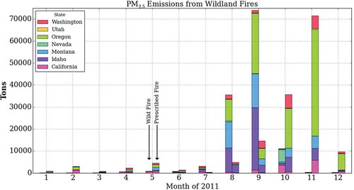
100% Fire (or with fire) case: Includes all the prescribed burn emissions in the domain as per NEI 2011 along with all other emissions for point, area, and mobile sources as used in daily AIRPACT forecasting.

30% Fire case: Includes all the prescribed burn sources as per NEI 2011, but all prescribed burn emissions and heat flux) are uniformly reduced by 70%, with other emissions the same as for the 100% fire case. This case reflects the harvesting of residue biomass for use as a potential feedstock for the aviation biofuel supply chain. This assumption is based on Perez-Garcia et al. (2012) and Pierobon, Eastin, and Ganguly (2018), which assume that of the total woody residue left in the forests, 65% is collected in the form of slash piles and 35% is left scattered in the forest. We assume that the biofuel production will reduce the need for burning, forming the basis of this case where we assume that 30% biomass is burned. While these numbers are for Washington, we uniformly apply these to the study domain. For calculating the emissions, a key assumption here is that a reduction in biomass will linearly reduce emissions and other related quantities. This is reasonable, considering that we are reducing the burn area.

No fire case: No prescribed burn emissions, and other emissions are kept same as the first case described. This case is the baseline against which the other two cases are compared.

Model evaluation methods

To address our first question on model performance, we evaluated the model for the with fire and no fire cases using conventional model performance measures as listed in Table 1. Model performance for the two scenarios is compared using mean fractional bias (MFB) and mean fractional error (MFE) and their comparison with the performance goals and performance criteria for PM_2.5. These performance goals (the best expected performance of a model) and criteria (acceptable level of model performance) were proposed by Boylan and Russell (2006) and were based on analysis of several modeling studies performed throughout the United States. We also compare the model performance using the normalized mean bias and error (NMB/E) goals and criteria established by (2017). Emery et al. We used two different observation datasets for the purpose of model evaluation: the Interagency Monitoring of Protected Visual Environments (IMPROVE) network (Malm et al. 1994) and USEPA’s AQS dataset. AQS provides hourly PM_2.5 concentrations for urban areas across the United States. IMPROVE sites are usually located in or near class I areas and measure the concentration of PM_2.5 and other PM_2.5 species, such as organic carbon (OC), elemental carbon (EC), sulfate (SO₄), nitrate (NO₃), and ammonium (NH₄). IMPROVE sites report 24-hr average concentrations with a frequency of once every 3 days. For visibility investigation we use the deciview (dv) metric (defined in the following), a preferred metric in the regional haze rule because a unit change in deciviews is unbiased by the prevailing visibility being highly impaired or clean (Pitchford and Malm 1994).

For IMPROVE sites, the concentrations of various PM_2.5 species are used with their corresponding coefficients of extinction to get the total extinction coefficient (called the reconstructed extinction coefficient) using the following equation (Pitchford et al. 2007):

(1) $\begin{array}{rl}& {\beta }_{ext}=2.2f_S\left(RH\right)\left[AMSU{L}_s\right]+4.8f_L\left(RH\right)\left[AMSU{L}_L\right]\\ & +2.4f_S\left(RH\right)\left[AMNI{T}_s\right]+5.1f_L\left(RH\right)\left[AMNI{T}_L\right]\\ & +2.8f_S{\left(RH\right)}_{OM}\left[O{M}_s\right]+6.1f_L{\left(RH\right)}_{OM}\left[O{M}_L\right]\\ & +1.7f{\left(RH\right)}_{SS}\left[P{M}_{2.5}SeaSalt\right]+1.0\left[P{M}_{2.5}Soil\right]\\ & +0.6\left[CoarseMass\right]+10\left[EC\right]+0.33\left[N{O}_2\left(ppb\right)\right]\\ & +{\beta }_{\mathrm{R}\mathrm{a}\mathrm{y}}\end{array}$(1)

where [AMSUL], [AMNIT], [OM], [EC], [Soil], [Sea Salt], [Coarse Mass], and [NO₂] are the concentrations (in μg/m³) of ammonium sulfate, ammonium nitrate, organic mass, elemental carbon, soil, sea salt, coarse PM, and NO₂, respectively. The f(RH) is a dimensionless relative humidity adjustment factor, needed to account for effect of water uptake by aerosols on the dry extinction coefficient. Several components in the preceding equation are divided in small and large modes, each with a separate relative humidity (RH) adjustment factor. The Rayleigh extinction coefficient, β_Ray, accounts for scattering by air molecules. The revised IMPROVE equation assumes that organic matter is not hygroscopic (f_S(RH) = f_L(RH) = 1), and the OM/OC ratio is 1.8. Lowenthal and Kumar (2016) recently evaluated the revised IMPROVE equation based on data collected from field studies, and recommended that OM should be considered hygroscopic and the OM/OC ratio of 2.1 should be used. Based on their recommendations, we use the OM/OC ratio of 2.1 and assume OM to be hygroscopic. The relative humidity adjustment factors for our analysis were taken from Lowenthal and Kumar (2016). The calculated β_ext is converted to deciviews using eq 2:

(2) $dv=10\ast \mathrm{l}\mathrm{n}\left({\beta }_{ext}/10\right)$(2)

Estimating the health benefits

To obtain the health impact estimates from different scenarios, we utilize the Benefits Mapping and Analysis Program Community Edition version 1.1 (BenMAP CE; https://www.epa.gov/benmap, developed by the USEPA), which contains various PM_2.5 mortality and morbidity concentration–response (C-R) functions, population data sets, incidence rates, and population growth functions. BenMAP can thus be used to estimate the health effects of different scenarios for different health endpoints. The generic form of a health impacts function, which relates the changes in the incidence of a health endpoint to the change in a pollutants concentration, can be written as (Fann et al. 2012)

(3) $\mathrm{\Delta }y=y_o\left[exp\left(\beta \ast \mathrm{\Delta }x\right)-1\right]\ast population$(3)

where y_o is the baseline incidence rate, β is the mortality or morbidity effect estimate (i.e., an estimate of the percent change in mortality or morbidity caused by a unit change in ambient concentration of the pollutant), Δx is change in pollutant concentration, and population is the population affected by the changed concentration (Fann et al. 2012). Baseline incidence rates for this analysis use the incidence data set contained within BenMAP. For the current analysis, Δx is taken as the concentration difference between the 100% fire and no fire cases, and the concentration difference between the 100% fire and 30% fire cases. The Δy from these two scenarios will give the health effects of prescribed fires and benefits for different health endpoints considered for this study when emissions are reduced. We consider a wide spectrum of health endpoints for which C-R functions are available in BenMAP. We also derived the effect estimate for fire specific studies for two health endpoints: all cardiovascular hospital admissions, and all respiratory hospital admissions based on Delfino et al. (2009). While there are several fire specific health studies that can be used to derive the effect estimate for other health endpoints, we avoid doing so because most of these studies were conducted outside of the United States, caveats of which are also explained in Fann et al. (2018).

BenMAP requires a full year of data for pollutant concentrations at each of the grid cells, and our current simulations covered only two months. To overcome this, we used the model simulations from a different year (May–September 2009, December 2009–April 2010; no fire emissions were included in these simulations) and concatenated it with the current simulations (October–November 2011). While this is not the best approach, we consider this to be acceptable considering that we are investigating the health impacts only from prescribed fires, for which emissions (and hence population exposure) maximize during the October–November time-period.

Results and discussion

Model performance evaluation and impact of prescribed fire on model performance

We show the impact of prescribed fires on model performance by calculating various standard metrics (Table 1) for both the 100% fire case and the no fire case. Comparison of various statistical metrics for 100% fire and no fire cases is shown for both IMPROVE and AQS sites in Table 2. The mean concentration at urban sites is much larger (8.4 µg/m³) compared to the nonurban IMPROVE sites (2.8 µg/m³). For the case when fire emissions are not included, the model underpredicts mean concentrations at both IMPROVE and AQS sites, whereas including fire emissions results in overprediction of mean concentration at both networks. While the fractional bias indicates improvement in performance when fire emissions are considered at the two networks, there is almost no change for the fractional error, indicating that large variability between modeled and observed concentrations still exists. Figure 2 shows how the model performance changes as a function of the observed concentration. The coefficient of correlation improves for both the networks for the 100% fire case, but the improvement is much more significant for IMPROVE sites. We also notice that, in general, the model overpredicts at lower observed concentration and underpredicts at higher observed concentration. Though including fire emissions improves the modeled concentration at higher observed concentrations, the underprediction is more severe at higher observed values, and more so at AQS sites; this could be attributed in part to the urban nature of sources, where the emissions from various sources such as vehicular emissions may not be captured completely. The bugle plots in Figure 3 show how the two different networks perform with respect to the performance goals and criteria. Most of the IMPROVE sites are within the performance criteria, with a few more sites within criteria with fire emissions included compared to the no fire case. While more sites are within criteria for the 100% fire case, including fire emissions results in overprediction at few sites where the average concentration is large. The new set of recommendations for model performance goals and criteria by Emery et al. (2017) uses NMB, NME, and the correlation coefficient (r). While recommended benchmarks for NMB and NME are specified for total PM_2.5 and for sulfate, ammonium, nitrate, organic carbon, and elemental carbon in the Emery et al. study, they only specify goals and criteria for r for total PM_2.5, sulfate, and ammonium. Our analysis does not use any concentration thresholds for total PM_2.5 or SO₄, NH₄, NO₃, OC, or EC. We find that NMB for PM_2.5 at AQS sites is −10% for the no fire simulations, which is within the NMB goal of ±10%, but increases to 17% for the fire simulations, which is still within the recommended criteria. With the PM_2.5 NME at AQS sites of 62% for the no fire case and 71% for the 100% fire case, the model doesn’t meet either the NME goal or the criteria for any of the simulation scenarios. At the IMPROVE sites, PM_2.5 NMB is −26%, which is within the criteria of ±30% for the no fire case, but 39% for the 100% fire case.

Table 2. Performance metrics for PM2.5 at the AQS and IMPROVE sites.

	AQS sites			IMPROVE sites
Metric	No fire	Fire		No fire		Fire
Number of observed–modeled pairs	6561			537
Mean observed (µg/m^3)	8.41			2.83
Mean modeled (µg/m^3)	7.54		9.82	2.06		3.88
MB (µg/m^3)	−0.87		1.41	−0.74		1.11
ME (µg/m^3)	5.17		5.94	1.55		2.12
MFB (%)	−19		1	−21		19
MFE (%)	61		59	57		54
NMB (%)	−10		17	−26		39
NME (%)	62		71	55		75
RMSE	7.71		9.42	2.81		4.16

Figure 2. Modeled to observed ratio versus observed PM_2.5 concentrations for AQS and IMPROVE sites.

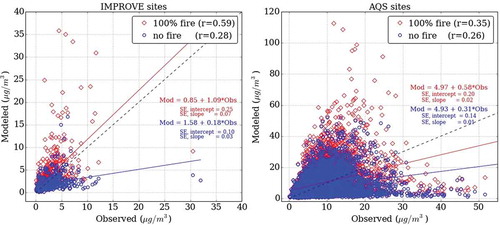
Figure 3. Bugle plots for comparison of MFB and MFE with goals and criteria for PM_2.5 during the period of simulation.

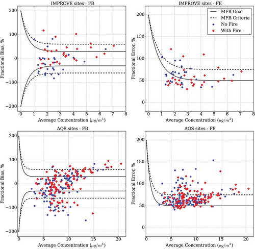
The speciated data in Table 3 show that organic carbon (OC) is the most dominant species, with a mean observed concentration of 1.21 µg/m³, and the performance is significantly improved with the bias changing from −0.74 µg/m³ for no fire to 0.06 µg/m³ for the 100% fire case and the corresponding fractional bias changing from −105% to only −17%. Compared to the no fire scenario when almost 50% sites are outside MFB performance criteria for OC, including prescribed fire emissions results in MFB within performance criteria for all the sites. For EC, SO₄, and NO₃, observed concentrations are much smaller compared to OC, and the model underpredicts in the no fire case and overpredicts in the 100% fire case. The concentrations for other species are small and remain within criteria in both the cases, since the MFB (MFE) approaches ±200% (200%) at very low concentrations. Table 3 also has NMB and NME for sulfate, nitrate, and elemental carbon, and we find that the model performance is relatively poor for these species for both the 100% fire and no fire cases. However, the model performance improves significantly for OC, for which NMB is 5% for the 100% fire simulations, compared to −81% for the no fire simulations, though the NME for both simulation scenarios is much larger compared to NME goals/criteria. Model ability to predict ammonium also improves for the 100% fire simulations, where the NMB is 10%, compared to −29% for the no fire simulations, which barely meets the criteria. Improved performance for OC and NH₄ is important, because these combined together account for 48% of the observed PM_2.5 mass concentration on average at the IMPROVE sites. The correlation coefficient, r, is shown in Figure 2 and is within the criteria for IMPROVE sites for total PM_2.5, but smaller than the recommended criteria at the AQS sites; nevertheless, there is an improvement is model performance during the 100% fire simulations compared to the no fire simulations.

Table 3. Performance metrics at the IMPROVE sites.

			With fire						No fire
Species	Number observed	Mean observed (µg/m^3)	Bias (µg/m^3)	MFB (%)	MFE (%)	NMB (%)	NME (%)	RMSE (µg/m^3)	Bias (µg/m^3)	MFB (%)	MFE (%)	NMB (%)	NME (%)	RMSE (µg/m^3)
OC	490	1.21	0.06	−17	73	5	75	4.68	−0.74	−105	114	−26	55	4.46
EC	488	0.17	0.18	46	75	110	160	0.76	−0.98	−33	73	−43	55	0.49
SO4^2-	502	0.33	0.20	55	66	61	78	0.33	−0.07	42	59	36	62	0.26
NH4^+	502	0.16	0.02	−4	64	10	71	0.19	0.12	−35	69	−29	58	0.13
NO3^−	502	0.14	0.19	48	100	141	183	0.49	−0.05	22	94	64	122	0.31

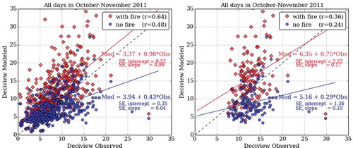
The scatter diagram in Figure 4 shows the deciview comparison at various IMPROVE sites for all the days in October–November 2011, as well as for the 20% highest deciview days. The model does better when fire emissions are included, with a correlation coefficient (r) of 0.51. This value is comparable to evaluations from Mebust et al. (2003), who reported r = 0.49, although they used a different observational data set. The performance is relatively poorer for the 20% days with worst visibility when compared to all the days in the simulation period, with the coefficient of correlation equal to 0.27. The mean observed deciview and mean bias for all days were 8.22 dv and 2.72 dv, respectively. For the 20% worst and 20% best visibility days, the mean observed deciview (and mean bias) were 12.70 dv (−4.95 dv) and 2.80 dv (0.08 dv), respectively. These differences can in part be attributed to the model’s ability to correctly reproduce the observed concentrations, as well as to the artifacts associated with the measurement of various PM_2.5 components (Mebust et al. 2003).

Figure 4. Modeled and observed deciview comparison for all days and 20% worst visibility days within the simulation period.

Overall, these results are comparable to previous studies using a 12-km version of AIRPACT conducted in the region during wildfire periods. Herron-Thorpe et al. (2014) reported that fractional bias for PM_2.5 at the AQS sites was ~−30% (FE of ~60%) for the simulations conducted for wildfire periods in 2007–08. While Herron-Thorpe et al. (2014) reported a mean bias of −0.72 µg/m³ for AQS sites, Chen et al. (2008) reported an overprediction of 2.1 and 2.2 µg/m³ at the AQS and IMPROVE sites, respectively. In general, we see that while some statistical metrics improve when fire emissions are considered, for some sites, fires cause large overprediction in the concentrations. This can be influenced by several factors, including the meteorological model failing to predict wind speed and direction correctly, application of a common temporal profile for all fires emissions, poorly simulated plume rise, and the complex topography in areas of prescribed fire. Additionally, it has been shown that the spatiotemporal allocation of the fires can also have a significant influence on the concentrations (Garcia-Menendez, Yongtao, and Odman 2014).

Regional and local impacts of prescribed fires

Figure 5a shows the concentration difference between the 100% fire and no fire cases for PM_2.5. Regional impacts of prescribed fires are most significant in the western part of the domain, especially in Oregon, where the average contribution from prescribed fires over the entire simulation period is ≥5 µg/m³ PM_2.5. This is somewhat expected, since maximum emissions from prescribed fires occur in Oregon (Figure 1). The difference is even larger for some areas, and peak concentration differences are greater than 20–25 µg/m³ in areas west of the Cascade mountain range. Emissions from prescribed fires contribute to PM_2.5 loading in excess of 5 µg/m³ for parts of northern Idaho as well as western Montana. A comparison of the simulation period average PM_2.5 concentrations between the 100% fire and no fire cases showed that total PM_2.5 loading in northern Idaho during this period is almost entirely attributable to prescribed fire emissions. Figure 5b shows the modeled relative change between 100% fire and 30% fire cases, which shows the potential benefits of avoiding biomass burning, and hence depicts the air quality benefits if the biomass is harvested for subsequent biofuel production. Only those model grid cells where the simulation period average for the 100% fire case was greater than 12 µg/m³ were considered. Large air quality benefits occur through PM_2.5 concentrations decreasing by more than 50−75% (6 µg/m³ or more) for most of the region in western Oregon. Large population centers around the interstate highway 5 (I-5) corridor also see up to 20% changes (1.8–2.4 µg/m³). Figure 5b is sensitive to the threshold concentration chosen for the 100% fire case, and changing this threshold to 8 or 10 µg/m³ results in more areas in Washington as well as northern Idaho showing improvements. The simulated changes are not directly proportional to the changes in emissions since reduced heat fluxes for the 30% biomass burn scenario will result in lower plume rises and thereby in reduced dispersion, which will cause larger near-source impacts for the same amount of emissions. While the simulated effects on PM_2.5 were significant during the period of simulation, a similar analysis didn’t show any contributions of prescribed fires to O₃, perhaps due to reduced photochemistry during the months of October–November. The 8-hr average O₃ concentration differences were very small (<1 ppb) at all the AQS sites considered, and so not of interest for further analysis.

Figure 5. (a) PM_2.5 difference between the 100% fire case and the no fire case when averaged over all days in the simulation period. (b) Percent change in PM_2.5 concentrations when all the fire emissions are uniformly reduced by 70%. Results for only those model grid cells where PM_2.5 concentrations for 100% fire case is greater than 12 μg/m³ are shown.

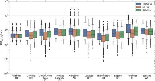
To consider the local impacts of prescribed fires, we identified several monitoring locations within the domain where air quality impacts occurred (Figure 6) and apply the relative response factors to observed PM_2.5 concentration to calculate the no fire case and 30% fire case concentrations. At several sites, such as Pinehurst (located in West Silver Valley, part of Idaho’s Shoshone County PM_2.5 non-attainment area) and Oakridge (a non-attainment region in Oregon), where prescribed fires are significant sources of PM_2.5, the 30% fire case causes the peak concentration to decrease significantly. Maximum hourly concentration changed from 111 μg/m³ to 60 μg/m³ for Pinehurst, and from 90 μg/m³ to 66 μg/m³ for Oakridge. For sites located near large populated areas, such as Portland, Eugene, and Vancouver, the average concentration is 10–11 μg/m³, and the maximum hourly concentration is 50 μg/m³, 71 μg/m³, and 278 μg/m³ in the 100% fire case, respectively. At all these places, the hourly peak concentration decreases by 5–10 μg/m³ in the 30% fire case. At several other sites not shown in the figure, such as Chester (CA), St. Maries (ID), and Kootenai Tribe (ID), where the mean concentration is otherwise very small, prescribed fire causes the mean and maximum concentrations to increase by an order of magnitude. Time-series plots at the sites indicate that while some communities are affected by elevated PM_2.5 concentrations only for a few specific days, others are affected frequently during the burn season. The time series also indicate that at urban sites, the impacts from prescribed fires are small and only for specific hours, indicating that the smoke management agencies are indeed successful in avoiding exposure to these large and urban population centers. In general, results at several of these sites that are located in small communities show that prescribed fires can impact air quality significantly and can be detrimental to the health of specific age groups or sensitive populations, and thus, a decrease in burning will represent significant air quality benefits for these small communities.

Figure 6. PM_2.5 distributions at selected sites for the three different scenarios. Whiskers represent 2nd and 98th percentiles.

Health effects of prescribed fires and benefits from avoided emissions

Using BenMAP, we calculated the health effects for two different control cases, the no fire and 30% fire cases, with respect to the base case (i.e., the 100% fire case). Table 4 shows the health impact estimates for these two cases. The mean number of additional mortalities caused by PM_2.5 from prescribed fire is ~280 for C-R functions from Krewski et al. (2009) and Pope et al. (2002), and ~710 deaths based on C-R functions from Laden et al. (2006), and these numbers decrease to ~200 and ~500, respectively, when prescribed fires are reduced by 70%. Additional mortality in both control cases is almost double for Laden et al. (2006) relative to Pope et al. (2002) or Krewski et al. (2009). This difference in the PM-caused mortality estimate is because of different effect estimates used in C-R functions. Estimates based on these studies are of long-term mortality. For quantifying short-term mortality due to smoke exposure from prescribed fires, we used the effect estimate from Zanobetti and Schwartz (2009). Based on Zanobetti and Schwartz (2009), an estimated 49 all-cause mortalities occur due to PM_2.5 from prescribed fires, and this number can be reduced to 34 for the scenario of reduced prescribed fires.

Table 4. Impact estimates for various health endpoints for no fire and 30% fire case (control cases) with 100% fire case (base case).

Health endpoint	Author	Impact estimate Δy = y100% Fire – yNo Fire	Impact estimate Δy = y100% Fire – y30% Fire
Mortality (all cause)	Krewski et al. (2009)	277	196
	Laden et al. (2006)	707	501
	Pope et al. (2002)	277	196
	Zanobetti and Schwartz (2009)	49	34
Acute bronchitis	Dockery et al. (1996)	398	283
Acute myocardial infarction (nonfatal)	Sullivan et al. (2005)	19	14
	Zanobetti et al. (2009)	22	16
Asthma exacerbation (cough)	Mar et al. (2004)	79,878	59,311
Asthma exacerbation (shortness of breath)	Mar et al. (2004)	26,972	20,371
Chronic bronchitis	Abbey et al. (1995)	190	135
Emergency-room visits (asthma)	Mar, Koenig, and Primomo (2010)	125	90
	Slaughter et al. (2005)	67	48
Hospital admissions all cardiovascular (less myocardial infarctions)	Bell et al. (2008)	24	17
	Peng et al. (2009)	21	15
	Delfino et al. (2009)	47	33
Hospital admissions all respiratory	Zanobetti et al. (2009)	49	35
	Delfino et al. (2009)	124	87
Lower respiratory symptoms	Schwartz and Neas (2000)	4,386	3,294
Upper respiratory symptoms	Pope et al. (1991)	7,286	5,186
Minor restricted activity days	Ostro and Rothschild (1989)	207,588	150,042
Work loss days	Ostro (1987)	35,662	25,568

Impacts for a number of other health endpoints are also considered, such as acute bronchitis, acute myocardial infarction (nonfatal heart attack), asthma, chronic bronchitis (irritation or inflammation of lung airways), emergency-room visits, hospital admissions, lower respiratory symptoms (LRS; defined as two or more of cough, chest pain, phlegm, or wheeze), upper respiratory symptoms (URS; defined as one or more of the following symptoms: runny or stuffy nose, wet cough, and burning, aching, or red eyes), and two additional endpoints indicative of the overall loss in productivity: minor restricted activity days and lost workdays. Based on our results (Table 4), more than 100,000 asthma cases, 400 acute bronchitis cases, 100–200 chronic bronchitis cases, 65–70 emergency-room visits, and 20–40 hospital admissions can be attributed to additional PM_2.5 concentrations caused by prescribed fires. When effect estimates derived from smoke-specific studies are used in the C-R functions, an estimated 124 cases of hospital admissions due to respiratory issues and 47 of hospital admissions due to cardiovascular diseases can be attributed to prescribed fires. Prescribed fires are also expected to contribute to 7300 additional URS and 4400 LRS cases, which are reduced by 29% and 25% for 30% fire cases. Most significant is workday losses or days of restricted activity (35,000 and 200,000+, respectively). In a reduced prescribed burning scenario, we see an improvement for all health endpoints, but the improvement is not proportional to the reduction in emissions. While emissions are reduced by 70%, calculated decrease in health impacts for various endpoints is only 25–30%. We believe that this is partly due to our assumption where the larger burns that are more buoyant and dispersed to longer distances are uniformly reduced in size, and the resulting smaller burns are not dispersed as much because of lower plume buoyancy.

The state-wise distribution of two different health endpoints—all cause mortality and asthma exacerbation—is shown in Figure 7. The effects are maximum for Oregon and Washington, but a reduction in prescribed burn results in fewer deaths or a reduction of diseases across the domain. While the air quality benefits from fire reduction are most prominent for Lincoln and Benton counties in Oregon, BenMAP shows maximum health benefits in the counties of Multnomah, Lane, Clackamas, and Washington counties in Oregon and King and Clark counties in Washington. These larger benefits are due to larger populations in these counties.

Figure 7. Prescribed fire attributed additional asthma attacks and mortality cases for various states in AIRPACT-4 model domain.

Impacts on visibility in class I areas

To assess the visibility benefits for class I areas that can be attributed to the reduction in prescribed fire emissions, we extracted the deciview data for the grid cells having at least 50% of the grid cell area within a national park and/or wilderness area. CMAQ outputs hourly deciview, but the IMPROVE network uses 24-hr average concentration, along with the relative humidity factor, and reports one deciview metric per day. To get a daily deciview metric from CMAQ, we used the daily average concentrations for ammonium sulfate, ammonium nitrate, elemental carbon, organic aerosols, and fine soil concentrations, with the relative humidity factor calculated using the daily average relative humidity (RH).

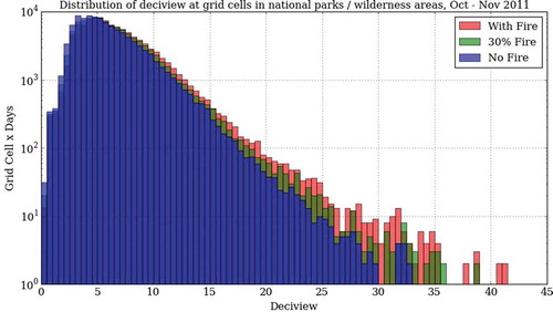
The distribution of the daily average deciview for the three different modeling scenarios is shown in Figure 8. We can derive two important results from this: (1) Fires impact the deciview distribution at both low deciviews (i.e., best visibility) and high deciviews (i.e., worst visibility); and (2) as we move to higher deciviews, many more grid cells are influenced by fires and the highest deciviews solely occur because of fires. This is indicative of the poor visibility in partial areas of national parks/wilderness areas, which may not be captured by monitoring at specific locations through the IMPROVE network. Our analysis indicates that almost all national parks and/or wilderness areas are affected at deciview extremes, except the North Cascades National Park, the Sawtooth National Forest, Olympic National Park, Mountain Rainier, and Sula Peak.

Figure 8. Deciview distribution for the grid cells in class I areas for the three emission scenarios.

To analyze the change in visibility from fire emission reduction from a regulatory perspective, the regional haze rule approach of reasonable progress toward achieving the goal of natural visibility is followed here: improving the most impaired visibility days (i.e., 20% worst visibility days or haziest days) while not degrading the visibility on cleanest days during a year. The concentrations of various species required for calculated the reconstructed extinction coefficient were obtained from IMPROVE network for 2011. For each site in the AIRPACT domain (n = 26), the deciviews were calculated using eq 2, assuming hygroscopic organic aerosols. From this new deciview data, the cleanest and haziest 20% days were extracted. Using the deciviews during these cleanest and haziest 20% days, a relative response factor (RRF; USEPA 2014) was calculated for each of the components in eq 2, except for NO₂ and sea salt. However, when projecting the deciviews to the no fire and 30% fire cases, we applied the component specific RRFs only for the days in October–November 2011. We did this since a reduction will not affect the visibility during other times of the year when there are no prescribed fires. Thus, we created a deciviews time series at each IMPROVE network site in the following manner for the 20% cleanest and haziest days:

(4) $d{v}_{site,day}=\left\{\begin{array}{c}{\left(d{v}_{RRF}\right)}_{site,day}ifdayinsimulationperiod\\ {\left(d{v}_{obs}\right)}_{site,day}ifdaynotinsimulationperiod\end{array}\right.$(4)

where dv_RRF is the RRF-based deciview and dv_obs is the observed deciview.

Average improvements in visibility for the 20% haziest days for each IMPROVE site are shown in Table 5. Sites where difference in deciview metric between the 100% fire and no fire or 30% fire case is comparable to the slope of Theil trend line (visibility trend at each site over the observed data set for 20% worst and best days; obtained from http://views.cira.colostate.edu/fed/siteBrowser/Default.aspx) are shown in bold. Our results show that at six sites (Columbia River Gorge, Monture, Craters of the Moon, Cabinet Mountains, Lava Beds, and Crater Lake), a no fire scenario will result in visibility improvements equal to or faster than current rate of improvements for the haziest 20% days given by the Theil trend. We also predict visibility improvements for the 30% fire scenario, with the largest rate of benefits for Monture, Glacier National Park, Crater Lake, Kalmiopsis, Cabinet Mountains, and Lava Beds. At Lava Beds and Crater Lake, the visibility improvements in the 30% fire scenario are also greater than the current rate of improvements given by the Theil trend. While we did see benefits from prescribed fires for the haziest 20% days, we did not see much difference for the cleanest 20% of the days and hence those are not reported here. These results show that even though prescribed fires are events planned to minimize smoke exposure, they contribute to impaired visibility in the protected natural environments, and their reduction via feedstock harvesting can improve visibility.

Table 5. Changes in average deciviews for the haziest 20% days during October–November 2011 at IMPROVE sites. Sites where the deciview improvements for the recued fire case are comparable with the Theil trend are shown in bold.

Site name	Site code	Deciview for 100% fire case	delta dv 100 % fire – No fire	delta dv 100% fire – 30% fire	Theil trend (dv/year)
Columbia River Gorge	CORI1	20.87	−0.13	−0.05	−0.10
Columbia Gorge #1	COGO1	19.42	−0.01	−0.02	−0.50
Three Sisters wilderness	THSI1	18.74	−0.09	−0.04	−0.10
Glacier NP	GLAC1	18.17	−0.17	−0.07	−0.18
Redwood NP	REDW1	17.93	−0.08	−0.03	−0.17
Mount Rainier NP	MORA1	16.97	0.00	0.00	−0.34
Starkey	STAR1	16.85	−0.16	−0.05	−0.44
Kalmiopsis	KALM1	16.85	−0.13	−0.06	−0.14
Hells Canyon	HECA1	16.49	−0.11	−0.05	−0.16
Mount Hood	MOHO1	16.26	−0.09	−0.04	−0.16
Trinity	TRIN1	16.15	−0.04	−0.02	−0.16
Snoqualmie Pass	SNPA1	15.96	−0.07	−0.03	−0.28
Monture	MONT1	15.94	−0.19	−0.09	−0.10
Flathead	FLAT1	15.77	−0.13	−0.06	−0.32
Olympic	OLYM1	15.77	−0.02	−0.01	−0.28
Craters of the Moon NM	CRMO1	15.01	−0.04	−0.02	−0.04
Lassen Volcanic NP	LAVO1	14.92	−0.07	−0.03	0.02
Cabinet Mountains	CABI1	14.65	−0.13	−0.06	−0.08
Sula Peak	SULA1	14.49	−0.01	0.00	0.00
Lava Beds NM	LABE1	13.59	−0.13	−0.06	−0.05
Crater Lake NP	CRLA1	13.48	−0.16	−0.07	−0.06
North Cascades	NOCA1	13.38	−0.01	0.00	0.00
Pasayten	PASA1	13.21	−0.06	−0.03	−0.29
Sawtooth NF	SAWT1	12.75	−0.01	0.00	−0.13
Gates of the Mountains	GAMO1	11.51	−0.03	−0.01	−0.01
White Pass	WHPA1	11.38	−0.10	−0.04	−0.11

Conclusion

In this study, we have considered the role of emissions from prescribed fires used for fuel management on model performance, regional and local air quality, visibility, and associated health impacts. We find that for the period of simulation, including the prescribed fire emissions improves the model performance both at urban AQS sites and at the rural IMPROVE network for several performance metrics. The mean observed PM_2.5 concentrations for the AQS and IMPROVE site were 8.41 µg/m³ and 2.83 µg/m³. When fire emissions are included in modeling we see an improvement in MFB and correlation coefficient; however, mean bias changes from −0.74 µg/m³ to 1.11 µg/m³ for IMPROVE sites (−0.87 µg/m³ to 1.41 µg/m³ for AQS sites) for the no fire and with fire cases, respectively, showing an overprediction in the mean concentration. However, when individual sites are considered, a small number of additional sites meet the MFB and MFE goals and criteria for PM_2.5 for the 100% fire scenario. Among PM species, maximum improvement occurs for OC, with performance significantly improving when simulating with all fire emissions. All sites were within criteria for EC, nitrate, sulfate, and ammonium aerosols in both the cases. When using the newer set of goals and criteria suggested by Emery et al. (2017) and based on NMB/NME, we see mixed results for the model performance. The model meets performance goals for PM_2.5 at AQS sites for the no fire case, while meeting criteria for the case where all fires are included. Similarly, at IMPROVE sites, the model starts overpredicting in the case where fire emissions are considered. Among speciated PM2.5, using the newer NMB/NME based goals and criteria, we find that model performance improves for organic carbon and ammonium, which form the bulk of PM_2.5 mass.

Our results show that a large part of the domain is affected by emissions from prescribed fires, with the most affected areas being western Oregon, northern Idaho, and western Montana. Under a scenario of 70% decrease in fire emissions (i.e., 70% avoided emissions when biomass is harvested for biofuels), we show that most of western Oregon and small areas in northern Idaho will see large decreases in average PM_2.5 concentrations. We have shown that while the impact from prescribed burning is small in more populated urban centers, for some small and tribal communities mean and peak concentrations can increase significantly, and these are the sites where a decrease in emissions can result in significant improvements in air quality. While our simulation period covers only a part of the year, results show that this reduction can also help some non-attainment and maintenance areas such as Pinehurst and Sandpoint in Idaho, where contributions from prescribed fires can be large. These indicate potential regional, as well as local, air quality benefits of avoided biomass burning and harvesting for a biofuel industry. Prescribed fires alone are expected to cause health impacts across an array of endpoints: 280–700 additional deaths, 4400 lower respiratory symptom cases, 7300 upper respiratory symptom cases, around 400 acute bronchitis cases, and several thousand workday losses, among others. A reduction of 70% in the prescribed fire emissions will benefit by reducing mortality and morbidity by 25–30% for most of the endpoints.

Prescribed fires also contribute to impaired visibility in the protected class I areas. Following the concept of regional haze rule, we derived the RRF for different modeling scenarios, and analyzed the effects of reduced fire emissions on the visibility in protected natural environments in the model domain. We have shown that a reduction in fire emissions will improve visibility at number of IMPROVE sites during the 20% worst visibility days, whereas the improvement is minimal for the cleanest 20% days.

We have seen that the model performance during the period of simulation is not very good. Also, in the absence of detailed data on slash pile burning across the region, we have used the prescribed burning emission inventory available from the USEPA for our analysis. The imperfect modeling results and other assumptions embedded in our analysis make the results uncertain. Despite these uncertainties, based on our analysis we can conclude that a reduction in prescribed burning emissions due to feedstock harvesting can have significant local and regional air quality benefits, especially at small rural and tribal communities, and can also be beneficial for current non-attainment parts in the domain and trying to meet the national ambient air quality standard. From a policy perspective, the benefits from avoided management fires can be significant for public health and present an opportunity toward accelerated improvement for visibility in protected natural environments.

Additional information

Funding

Funding for this work was provided by the Northwest Advanced Renewables Alliance (NARA) program, which is led by Washington State University and supported by the Agriculture and Food Research Initiative Competitive Grant number 2011-68005-30416 from the USDA National Institute of Food and Agriculture. The AIRPACT system used in this study is operated with support from NW-AIRQUEST (http://lar.wsu.edu/nw-airquest) and the Agriculture and Food Research Initiative, USDA National Institute of Food and Agriculture [2011-68005-30416].

Notes on contributors

Vikram Ravi

Vikram Ravi is a Ph.D. student in the Laboratory for Atmospheric Research, Department of Civil & Environmental Engineering, Washington State University, Pullman, WA.

Joseph K. Vaughan

Joseph K. Vaughan is a research associate professor in the Laboratory for Atmospheric Research, Department of Civil & Environmental Engineering, Washington State University, Pullman, WA.

Michael P. Wolcott

Michael P. Wolcott is a Regents Professor in the Department of Civil & Environmental Engineering and Director of the Institute for Sustainable Design, Washington State University, Pullman, WA.

Brian K. Lamb

Brian K. Lamb is a Regents Professor and Boeing Distinguished Professor of environmental engineering in the Laboratory for Atmospheric Research, Department of Civil & Environmental Engineering, Washington State University, Pullman, WA.

References

- Abbey, D. E., B. E. Ostro, F. Petersen, and R. J. Burchette. 1995. Chronic respiratory symptoms associated with estimated long-term ambient concentrations of fine particulates less than 2.5 microns in aerodynamic diameter (PM2.5) and other air pollutants. J. Expo. Anal. Environ. Epidemiol. 5 (2):137–159.
- Bell, M. L., K. Ebisu, R. D. Peng, J. Walker, J. M. Samet, S. L. Zeger, and F. Dominici. 2008. Seasonal and regional short-term effects of fine particles on hospital admissions in 202 US counties, 1999-2005. Am. J. Epidemiol. 168 (11):1301–1310. doi:10.1093/aje/kwn252.
- Boylan, J. W., and A. G. Russell. 2006. PM and light extinction model performance metrics, goals, and criteria for three-dimensional air quality models. JOUR. Atmospheric Environ. 40 (26):4946–4959. doi:10.1016/j.atmosenv.2005.09.087.
- Byun, D., and K. L. Schere. 2006. Review of the governing equations, computational algorithms, and other components of the models-3 community multiscale air quality (CMAQ) modeling system. JOUR. Appl. Mech. Rev. 59 (2):51–77. doi:10.1115/1.2128636.
- Byun, D. W., J. E. Pleim, R. T. Tang, and A. Bourgeois. 1999. Meteorology-Chemistry Interface Processor (MCIP) for models-3 Community Multiscale Air Quality (CMAQ) modeling system. JOUR. Washington DC US Environ. Prot. Agency, Off. Res. Dev, EPA/600/R-99/030.
- Carter, W. P. L. 2000. DDocumentation of the SAPRC-99 chemical mechanism for VOC reactivity assessment. Final Report to California Air Resources Board Contract 92-329 and Contract 95-308, Air Pollution Research Center and College of Engineering Center for Environmental Research and Technology, University of California Riverside, California. Available online at: https://www.engr.ucr.edu/~carter/reactdat.htm.
- Chen, J., J. Vaughan, J. Avise, S. O’Neill, and B. Lamb. 2008. Enhancement and evaluation of the AIRPACT ozone and PM 2.5 forecast system for the Pacific Northwest. J. Geophys. Res. 113 (D14):D14305. doi:10.1029/2007JD009554.
- Delfino, R. J., S. Brummel, J. Wu, H. Stern, B. Ostro, M. Lipsett, A. Winer, et al. 2009. The relationship of respiratory and cardiovascular hospital admissions to the Southern California Wildfires of 2003. Occup. Environ. Med. 66 (3):189–197. http://www.jstor.org/stable/27733098
- Dockery, D. W., C. Arden Pope, X. Xu, J. D. Spengler, J. H. Ware, M. E. Fay, B. G. Ferris, and F. E. Speizer. 1993. An association between air pollution and mortality in six U.S. cities. JOUR. New England J. Med. 329 (24):1753–1759. doi:10.1056/NEJM199312093292401.
- Dockery, D. W., J. Cunningham, A. I. Damokosh, L. M. Neas, J. D. Spengler, and P. Koutrakis. 1996. Health effects of acid aerosols on North American children: Respiratory symptoms. Environ. Health Perspect. 104 (5):500–505. doi:10.1289/ehp.96104500.
- Emery, C., Z. Liu, A. G. Russell, M. Talat Odman, G. Yarwood, and N. Kumar. 2017. Recommendations on statistics and benchmarks to assess photochemical model performance. J. Air Waste Manage. Assoc. 67 (5):582-598. doi: 10.1080/10962247.2016.1265027.
- Emmons, L. K., S. Walters, P. G. Hess, J.-F. Lamarque, G. G. Pfister, D. Fillmore, C. Granier, A. Guenther, D. Kinnison, T. Laepple, J. Orlando, X. Tie, G. Tyndall, C. Wiedinmyer, S. L. Baughcum, and S. Kloster. 2010. Description and evaluation of the model for ozone and related chemical tracers, version 4 (MOZART-4). Geosci. Model Dev. 3 (1):43–67. doi:10.5194/gmd-3-43-2010.
- Fann, N., A. D. Lamson, S. C. Anenberg, K. Wesson, D. Risley, and B. J. Hubbell. 2012. Estimating the national public health burden associated with exposure to ambient PM2.5 and ozone. Risk Anal. 32 (1):81–95. doi:10.1111/j.1539-6924.2011.01630.x.
- Fann, N., B. Alman, R. A. Broome, G. G. Morgan, F. H. Johnston, G. Pouliot, and A. G. Rappold. 2018. The health impacts and economic value of wildland fire episodes in the U.S.: 2008–2012. Sci. Total Environ. 610–611 (January):802–809. doi:10.1016/j.scitotenv.2017.08.024.
- Garcia-Menendez, F., H. Yongtao, and M. T. Odman. 2014. Simulating smoke transport from wildland fires with a regional-scale air quality model: sensitivity to spatiotemporal allocation of fire emissions. Sci. Total Environ. 493 (September):544–553. doi:10.1016/j.scitotenv.2014.05.108.
- Guenther, A. B., X. Jiang, C. L. Heald, T. Sakulyanontvittaya, T. Duhl, L. K. Emmons, and X. Wang. 2012. The model of emissions of gases and aerosols from nature version 2.1 (MEGAN2.1): An extended and updated framework for modeling biogenic emissions. Geosci. Model Dev. 5 (6):1471–1492. doi:10.5194/gmd-5-1471-2012.
- Haikerwal, A., F. Reisen, M. R. Sim, M. J. Abramson, C. P. Meyer, F. H. Johnston, and M. Dennekamp. 2015. Impact of smoke from prescribed burning: Is it a public health concern? J. Air Waste Manag. Assoc. 65 (5):592–598. doi:10.1080/10962247.2015.1032445.
- Herron-Thorpe, F. L., G. H. Mount, L. K. Emmons, B. K. Lamb, D. A. Jaffe, N. L. Wigder, S. H. Chung, R. Zhang, M. D. Woelfle, and J. K. Vaughan. 2014. Air quality simulations of wildfires in the pacific northwest evaluated with surface and satellite observations during the summers of 2007 and 2008. JOUR. Atmospheric. Chem. Phys. 14 (22):12533–12551. doi:10.5194/acp-14-12533-2014.
- Hu, Y., M. Talat Odman, M. E. Chang, W. Jackson, S. Lee, E. S. Edgerton, K. Baumann, and A. G. Russell. 2008. Simulation of air quality impacts from prescribed fires on an urban area. JOUR. Environ. Sci. Technol. 42 (10):3676–3682. doi:10.1021/es071703k.
- Kennard, D., K. Outcalt, D. Jones, and J. OBrien. 2005. Comparing techniques for estimating flame temperature of prescribed fires. J. Assoc. Fire Ecol. 1 (1):75–84. doi:10.4996/fireecology.0101075.
- Krewski, D., M. Jerrett, R. T. Burnett, R. Ma, E. Hughes, Y. Shi, M. C. Turner, et al. 2009. Extended follow-up and spatial analysis of the american cancer society study linking particulate air pollution and mortality. JOUR. Res. Rep. Health Eff. Inst. 140. Health Effects Institute, Boston, MA.
- Laden, F., J. Schwartz, F. E. Speizer, and D. W. Dockery. 2006. Reduction in fine particulate air pollution and mortality: Extended follow-up of the harvard six cities study. Am. J. Respir. Crit. Care Med. 173 (6):667–672. doi:10.1164/rccm.200503-443OC.
- Larkin, N. K., S. M. O’Neill, R. Solomon, S. Raffuse, T. Strand, D. C. Sullivan, C. Krull, M. Rorig, J. Peterson, and S. A. Ferguson. 2009. The bluesky smoke modeling framework. JOUR. Int. J. Wildland Fire. doi:10.1071/WF07086.
- Lelieveld, J., J. S. Evans, M. Fnais, D. Giannadaki, and A. Pozzer. 2015. The contribution of outdoor air pollution sources to premature mortality on a global scale. JOUR. Nature 525 (7569):367–371. doi:10.1038/nature15371.
- Lowenthal, D. H., and N. Kumar. 2016. Evaluation of the improve equation for estimating aerosol light extinction. J. Air Waste Manage Assoc. 66 (7):726–737. doi:10.1080/10962247.2016.1178187.
- Malm, W. C., J. F. Sisler, D. Huffman, R. A. Eldred, and T. A. Cahill. 1994. Spatial and seasonal trends in particle concentration and optical extinction in the United States. JOUR. J. Geophys. Res. 99:1347. doi:10.1029/93JD02916.
- Mar, T. F., J. Q. Koenig, and J. Primomo. 2010. Associations between asthma emergency visits and particulate matter sources, including diesel emissions from stationary generators in Tacoma, Washington. Inhal. Toxicol. 22 (6):445–448. doi:10.3109/08958370903575774.
- Mar, T. F., T. V. Larson, R. A. Stier, C. Claiborn, and J. Q. Koenig. 2004. An analysis of the association between respiratory symptoms in subjects with asthma and daily air pollution in Spokane, Washington. Inhal. Toxicol. 16 (13):809–815. doi:10.1080/08958370490506646.
- Mass, C. F., M. Albright, D. Ovens, R. Steed, M. MacIver, E. Grimit, T. Eckel, B. Lamb, J. Vaughan, K. Westrick, P. Storck, B. Colman, C. Hill, N. Maykut, M. Gilroy, S. A. Ferguson, J. Yetter, J. M. Sierchio, C. Bowman, R. Stender, R. Wilson, and W. Brown. 2003. Regional environmental prediction over the Pacific Northwest. JOUR. Bull. Am. Meteorol. Soc. 84 (10):1353–1366. doi:10.1175/BAMS-84-10-1353.
- Mebust, M. R., B. K. Eder, F. S. Binkowski, and S. J. Roselle. 2003. Models-3 Community Multiscale Air Quality (CMAQ) Model Aerosol Component 2. Model evaluation. J. Geophys. Res. 108 (D6):4184. doi:10.1029/2001JD001410.
- Naeher, L. P., G. L. Achtemeier, J. S. Glitzenstein, D. R. Streng, and D. Macintosh. 2006. Real-time and time-integrated PM2.5 and CO from prescribed burns in chipped and non-chipped plots: Firefighter and community exposure and health implications. JOUR. J. Expos. Sci. Environ. Epidemiol. 16 (4):351–361. doi:10.1038/sj.jes.7500497.
- NAPAP. 1991. 1990 Integrated Assessment Report. National Acid Precipitation Assessment Program. Washington, DC.
- Ostro, B. D. 1987. Air pollution and morbidity revisited: A specification test. J. Environ. Econ. Manage 14 (1):87–98. doi:10.1016/0095-0696(87)90008-8.
- Ostro, B. D., and S. Rothschild. 1989. Air pollution and acute respiratory morbidity: An observational study of multiple pollutants. Environ. Res. 50 (2):238–247. doi:10.1016/S0013-9351(89)80004-0.
- Otte, T. L., and J. E. Pleim. 2010. The Meteorology-Chemistry Interface Processor (MCIP) for the CMAQ modeling system: Updates through MCIPv3.4.1. Geosci. Model Dev. 3 (1):243–256. doi:10.5194/gmd-3-243-2010.
- Peng, R. D., M. L. Bell, A. S. Geyh, A. McDermott, S. L. Zeger, J. M. Samet, and F. Dominici. 2009. Emergency admissions for cardiovascular and respiratory diseases and the chemical composition of fine particle air pollution. Environ. Health Perspect. 117 (6):957–963. doi:10.1289/ehp.0800185.
- Perez-Garcia, J., E. Oneil, T. Hansen, T. Mason, J. McCarter, L. Rogers, A. Cooke, J. Comnick, and M. McLaughlin. 2012. Washington forest biomass supply assessment. Washington State Department of Natural Resources. Available at: http://file.dnr.wa.gov/publications/em_finalreport_wash_forest_biomass_supply_assess.pdf.
- Pierobon, F., I. L. Eastin, and I. Ganguly. 2018. Life cycle assessment of residual lignocellulosic biomass-based jet fuel with activated carbon and lignosulfonate as co-products. Biotechnol. Biofuels 11 (1):139. doi:10.1186/s13068-018-1141-9.
- Pitchford, M., W. Malm, B. Schichtel, N. Kumar, D. Lowenthal, and J. Hand. 2007. Revised algorithm for estimating light extinction from IMPROVE particle speciation data. J. Air Waste Manage Assoc. 57 (11):1326–1336. doi:10.3155/1047-3289.57.11.1326.
- Pitchford, M. L., and W. C. Malm. 1994. Development and applications of a standard visual index. Atmos. Environ. 28 (5):1049–1054. doi:10.1016/1352-2310(94)90264-X.
- Pope, C. A., D. W. Dockery, J. D. Spengler, and M. E. Raizenne. 1991. Respiratory health and PM10 pollution: A daily time series analysis. JOUR. Am. Rev. Respir. Dis. 144 (3_pt_1):668–674. doi:10.1164/ajrccm/144.3_Pt_1.668.
- Pope, C. A., M. J. Thun, E. E. Calle, D. Krewski, K. Ito, and G. D. Thurston. 2002. Lung cancer, cardiopulmonary mortality, and long-term exposure to fine particulate air pollution. JOUR. JAMA 287. doi:10.1001/jama.287.9.1132.
- Pyne, S. J., P. L. Andrews, and R. D. Laven. 1996. Introduction to wildland fire. Second. New York: Wiley.
- Raffuse, S. M., D. A. Pryden, D. C. Sullivan, N. K. Larkin, T. Strand, and R. Solomon. 2009. SMARTFIRE algorithm description. JOUR. US Environmental Protection Agency, Research Triangle Park, NC, by Sonoma Technology, Inc., Petaluma, CA, and the US Forest Service, AirFire Team, Pacific Northwest Research Laboratory, Seattle, WA STI-905517-3719.
- Ravi, V., A. H. Gao, N. B. Martinkus, M. P. Wolcott, and B. K. Lamb. 2018. Air quality and health impacts of an aviation biofuel supply chain using forest residue in the northwestern United States. Environ. Sci. Technol. 52 (7):4154–4162. doi:10.1021/acs.est.7b04860.
- Sandberg, D., R. Ottmar, J. Peterson, and J. Core. 2002. Wildland fire in ecosystems: Effects of fire on air. Gen. Tech. Rep. RMRS-GTR-42. Ogden, UT: U.S. Department of Agriculture, Forest Service, Rocky Mountain Research Station.
- Schwartz, J., D. W. Dockery, and L. M. Neas. 1996. Is daily mortality associated specifically with fine particles? J. Air Waste Manage Assoc. 46 (10):927–939. doi:10.1080/10473289.1996.10467528.
- Schwartz, J., and L. M. Neas. 2000. Fine particles are more strongly associated than coarse particles with acute respiratory health effects in schoolchildren. Epidemiology 11 (1):6–10. doi:10.1097/00001648-200001000-00004.
- Skamarock, W. C., J. B. Klemp, J. Dudhia, D. O. Gill, D. M. Barker, W. Wang, and J. G. Powers. 2005. A description of the advanced research WRF Version 2. RPRT. DTIC Document.
- Slaughter, J. C., E. Kim, L. Sheppard, J. H. Sullivan, T. V. Larson, and C. Claiborn. 2005. Association between particulate matter and emergency room visits, hospital admissions and mortality in Spokane, Washington. J. Expo. Anal. Environ. Epidemiol. 15 (2):153–159. doi:10.1038/sj.jea.7500382.
- Sullivan, J., L. Sheppard, A. Schreuder, N. Ishikawa, D. Siscovick, and J. Kaufman. 2005. Relation between short-term fine-particulate matter exposure and onset of myocardial infarction. Epidemiology 16 (1):41–48. doi:10.1017/CBO9781107415324.004.
- Tian, D., Y. Hu, Y. Wang, J. W. Boylan, M. Zheng, and A. G. Russell. 2009. Assessment of biomass burning emissions and their impacts on urban and regional PM2.5: A georgia case study. JOUR. Environ. Sci. Technol. 43 (2):299–305. doi:10.1021/es801827s.
- USEPA. 1998. Interim air quality policy on wildland and prescribed fires.
- USEPA. 1999. Regional haze regulations: Final rule. 40 CFR Part. 51; Fed. Regist. 64(126):35714–35774.
- USEPA. 2011. The 2011 National Emissions Inventory. https://www3.epa.gov/ttnchie1/net/2011inventory.html.
- USEPA. 2014. Modeling Guidance for Demonstrating Attainment of Air Quality Goals for Ozone, PM2.5 and Regional Haze. Available at https://www3.epa.gov/scram001/guidance/guide/Draft_O3-PM-RH_Modeling_Guidance-2014.pdf.
- Vaughan, J., B. Lamb, C. Frei, R. Wilson, C. Bowman, C. Figueroa-Kaminsky, S. Otterson, et al. 2004. A numerical daily air quality forecast system for the Pacific Northwest. JOUR. Bull. Am. Meteorol. Soc. 85 (4):549–561. doi:10.1175/BAMS-85-4-549.
- Wiedinmyer, C., B. Quayle, C. Geron, A. Belote, D. McKenzie, X. Zhang, S. O’Neill, and K. K. Wynne. 2006. Estimating emissions from fires in North America for air quality modeling. Atmos. Environ. 40 (19):3419–3432. doi:10.1016/j.atmosenv.2006.02.010.
- Wimberly, M. C., and Z. Liu. 2014. Interactions of climate, fire, and management in future forests of the Pacific Northwest. For. Ecol. Manage. 327 (September):270–279. doi:10.1016/j.foreco.2013.09.043.
- Zanobetti, A., and J. Schwartz. 2009. The effect of fine and coarse particulate air pollution on mortality: a national analysis. Environ. Health Perspect. 117 (6):898–903. doi:10.1289/ehp.0800108.
- Zanobetti, A., M. Franklin, P. Koutrakis, and J. Schwartz. 2009. Fine particulate air pollution and its components in association with cause-specific emergency admissions. Environ. Health 8:58. doi:10.1186/1476-069X-8-58.
- Zeng, T., Y. Wang, Y. Yoshida, D. Tian, A. G. Russell, and W. R. Barnard. 2008. Impacts of prescribed fires on air quality over the southeastern united states in spring based on modeling and ground/satellite measurements. JOUR. Environ. Sci. Technol. 42 (22):8401–8406. doi:10.1021/es800363d.