Spatial PM_2.5 mobile source impacts using a calibrated indicator method

ABSTRACT

Motor vehicles are major sources of fine particulate matter (PM_2.5), and the PM_2.5 from mobile vehicles is associated with adverse health effects. Traditional methods for estimating source impacts that employ receptor models are limited by the availability of observational data. To better estimate temporally and spatially resolved mobile source impacts on PM_2.5, we developed an approach based on a method that uses elemental carbon (EC), carbon monoxide (CO), and nitrogen oxide (NO_x) measurements as an indicator of mobile source impacts. We extended the original integrated mobile source indicator (IMSI) method in three aspects. First, we generated spatially resolved indicators using 24-hr average concentrations of EC, CO, and NO_x estimated at 4 km resolution by applying a method developed to fuse chemical transport model (Community Multiscale Air Quality Model [CMAQ]) simulations and observations. Second, we used spatially resolved emissions instead of county-level emissions in the IMSI formulation. Third, we spatially calibrated the unitless indicators to annually-averaged mobile source impacts estimated by the receptor model Chemical Mass Balance (CMB). Daily total mobile source impacts on PM_2.5, as well as separate gasoline and diesel vehicle impacts, were estimated at 12 km resolution from 2002 to 2008 and 4 km resolution from 2008 to 2010 for Georgia. The total mobile and separate vehicle source impacts compared well with daily CMB results, with high temporal correlation (e.g., R ranges from 0.59 to 0.88 for total mobile sources with 4 km resolution at nine locations). The total mobile source impacts had higher correlation and lower error than the separate gasoline and diesel sources when compared with observation-based CMB estimates. Overall, the enhanced approach provides spatially resolved mobile source impacts that are similar to observation-based estimates and can be used to improve assessment of health effects.

Implications: An approach is developed based on an integrated mobile source indicator method to estimate spatiotemporal PM_2.5 mobile source impacts. The approach employs three air pollutant concentration fields that are readily simulated at 4 and 12 km resolutions, and is calibrated using PM_2.5 source apportionment modeling results to generate daily mobile source impacts in the state of Georgia. The estimated source impacts can be used in investigations of traffic pollution and health.

Introduction

Ambient air pollution has been associated with human morbidity and mortality (Brauer et al. 2016; Kampa and Castanas 2008; Lelieveld et al. 2015; West et al. 2016). The relationship between adverse health effects and air pollution has been investigated using different types of pollutant concentration metrics, particularly single-pollutant metrics of fine particulate matter (PM_2.5) and nitrogen dioxide (NO₂) (Cohen et al. 2005; Kioumourtzoglou et al. 2016; Pope, Ezzati, and Dockery 2009; Zeger et al. 2008) and ozone (Chen et al. 2015; Uysal and Schapira 2003). Single-pollutant metrics are usually provided by ambient measurements, model simulations, or fusion of observation and simulation (Bates et al. 2018; Huang et al. 2018b, 2018a; Zhai et al. 2016). Variations in single pollutant levels may not fully capture the actual variations in human exposure to air pollution changes because populations are exposed to a complex mixture of pollutants. Health effects researchers are now concerned with multicomponent exposures and developing health effects models that account for multipollutant exposures and the resulting outcomes (e.g., Russell et al. 2018). Multipollutant metrics may be more representative of actual exposure and more directly related to source impacts. Studies have shown that multipollutant metrics are related to adverse health effects (Dominici et al. 2010; Hidy and Pennell 2010; Johns et al. 2012).

Multipollutant exposure has been estimated by different grouping methods, such as chemical and/or biological reactivity, health effects, and contributing sources (Chen and Lippmann 2009; Hart et al. 2011; Kim et al. 2007; Mauderly and Chow 2008; Oakes, Baxter, and Long 2014a; Pachon et al. 2012). Source impacts derived using source apportionment techniques are mixtures of pollutants that are directly related to air pollution controls (Gehring et al. 2010; Kelly and Fussell 2012; Maciejczyk and Chen 2005; Sarnat et al. 2008). Traffic-related pollution is of particular interest due to the ubiquity of the source, particularly in highly populated areas, and observed associations with various health effects (Beelen et al., 2014; Brauer et al. 2008; Chen et al. 2013; Gehring et al. 2010; Kelly and Fussell 2012; Nordling et al. 2008). Motor vehicles emit PM_2.5 constituents, such as elemental carbon (EC), organic carbon (OC), and trace metals, as well as gas-phase pollutants, such as carbon monoxide (CO) and nitrogen oxides (NO_x, referring to the sum of nitric oxide [NO] and nitrogen dioxide [NO₂]). These motor vehicle–related pollutants are associated with adverse health effects individually and in combination (Delfino et al. 2006; Kelly and Fussell 2012; Kennedy et al. 2018; Melen et al. 2008; Oakes et al. 2014b; Pachon et al. 2012; Pennington et al. 2017).

Source impacts can be estimated using receptor-based models, such as the Chemical Mass Balance (CMB) model (U.S. Environmental Protection Agency [EPA] 2004) and the positive matrix factorization (PMF) method (Paatero and Tapper 1994), and emission-based dispersion models and chemical transport models (CTMs), such as the Research LINE-source dispersion model (R-LINE) (Snyder et al. 2013) and Community Multiscale Air Quality (CMAQ) model with Decoupled Direct Method (CMAQ-DDM) (Napelenok et al. 2006). Receptor models for PM_2.5 are based on ambient measurements for PM_2.5 species, with or without predetermined source profiles (EPA 2004; Lee et al. 2008). Their dependence on spatially sparse measurements limits the spatial and temporal coverage of the estimates. Studies have improved the temporal coverage using the daily temporal interpolation method (Redman et al. 2016). More spatially and temporally comprehensive source impact metrics can be developed using CTMs (Held et al. 2005; Ivey et al. 2015; Napelenok et al. 2006). Those models have biases due to limitations in inputs and simulation, such as emissions, meteorology, and transport and chemistry specifications. Efforts to combine the receptor models with dispersion models and regional-scale CTMs (Hu et al. 2014; Ivey et al. 2015; Sturtz, Schichtel, and Larson 2014) reduce these biases but are computationally expensive.

Pachon et al. (2012) developed a straightforward emission-based integrated mobile source indicator (IMSI) using observed concentrations and estimated emissions of CO, NO_x, and EC to calculate a unitless indicator of mobile source impacts. The generated indicator is significantly correlated with health outcomes at multiple locations (Oakes et al. 2014b; Pachon et al. 2012). However, this unitless indicator does not provide information on spatial variation in source impacts.

In this paper, we extended the IMSI method to estimate daily mobile source impacts on PM_2.5 at 4 km and 12 km resolutions.

Methods

The IMSI method is extended from providing single-location, unitless indicators to providing spatially resolved daily mobile source impacts on PM_2.5. The update method uses concentration fields generated by fusing CMAQ fields with observational data, emission fields estimated for mobile source, and source impact data by receptor model (CMB). The approach is applied for estimating the total mobile, gasoline, and diesel source impacts on PM_2.5 in the state of Georgia in the United States from 2002 to 2008 at 12 km resolution and from 2008 to 2010 at 4 km resolution; these different resolutions are due to the differing availability of CMAQ results (Boothe et al. 2006).

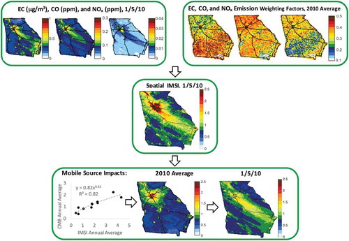
The overall approach is depicted in Figure 1 in four steps, with the output from each step shown in one block on the figure. First, daily 24-hr average concentration fields of EC, CO, and NO_x are obtained using the CMAQ–observation data fusion method (Friberg et al. 2016a). Pachon et al. (2012) used central site measurements of 1-hr maximum concentrations of CO and NO_x in developing the IMSI method. Here, we used 24-hr average concentrations for CO and NO_x to obtain daily mobile source impact estimates. Second, spatially resolved weighting factors are generated from emission data for combining the indicator species. Third, daily integrated mobile source indicator fields are derived. Finally, the unitless indicators are calibrated and converted to mobile source impacts using CMB annual source impacts. The methods and the data used are described in detail below. When calibrating the indicators to source impacts, we proposed an alternative approach, the local IMSI method, in addition to the main method. We found that the two methods yield similar results.

Figure 1. Procedure for estimating spatially and temporally resolved mobile source indicators.

Integrated mobile source indicator method

As EC, CO, and NO_x are mainly emitted by mobile sources, Pachon et al. (2012) postulated that their variations could be representative of mobile source impact changes. The IMSI method uses EC, CO, and NO_x concentrations as indicator species of mobile sources and mobile emission fractions (of total emissions) as weighting factors to combine them into a unitless indicator (eq 1). The IMSI method was also developed to estimate indicators of gasoline vehicle (GV) and diesel vehicle (DV) contributions separately (eqs 2 and 3, respectively). As EC is mostly contributed by diesel vehicles and CO is mostly contributed by gasoline vehicles, the DV indicator combines EC and NO_x concentrations and the GV indicator combines CO and NO_x concentrations.

In the IMSI method, daily 24-hr average species concentrations (C) observed at central sites are first normalized by their standard deviations (σ) over 1 yr. Then, these normalized values are averaged based on weighting factors (α) calculated from source emission estimates (E) that vary in space but not in time (eq 4 for the total mobile source indicator; eqs 5 and 6 for the GV and DV indicators, respectively). The weighting factors, which are in essence emission coefficients, are defined as the ratios of mobile source (GV/DV) emissions over total emissions for each species normalized by the sum of ratios over the three species. As such, these weighting factors do not vary over time and sum to 1 across the three species at each point in space for each source category (total mobile, GV, and DV). The IMSI indicators are normally distributed with a mean of the weighted average of the normalized concentrations (C/σ).

(1) $\mathrm{I}\mathrm{M}\mathrm{S}{\mathrm{I}}_{\mathrm{m}\mathrm{o}\mathrm{b}\mathrm{i}\mathrm{l}\mathrm{e}}={\alpha }_{EC}\times \frac{C_{\mathrm{E}\mathrm{C}}}{{\sigma }_{\mathrm{E}\mathrm{C}}}+{\alpha }_{CO}\times \frac{C_{CO}}{{\sigma }_{CO}}+{\alpha }_{\mathrm{N}\mathrm{O}\mathrm{x}}\times \frac{C_{\mathrm{N}\mathrm{O}\mathrm{x}}}{{\sigma }_{\mathrm{N}\mathrm{O}\mathrm{x}}}$(1)

(2) ${\mathrm{I}\mathrm{M}\mathrm{S}\mathrm{I}}_{GV}={\alpha }_{GV,CO}\times \frac{C_{CO}}{{\sigma }_{CO}}+{\alpha }_{GV,\mathrm{N}\mathrm{O}\mathrm{x}}\times \frac{C_{\mathrm{N}\mathrm{O}\mathrm{x}}}{{\sigma }_{\mathrm{N}\mathrm{O}\mathrm{x}}}$(2)

(3) ${\mathrm{I}\mathrm{M}\mathrm{S}\mathrm{I}}_{DV}={\alpha }_{DV,\mathrm{E}\mathrm{C}}\times \frac{C_{\mathrm{E}\mathrm{C}}}{{\sigma }_{\mathrm{E}\mathrm{C}}}+{\alpha }_{DV,\mathrm{N}\mathrm{O}\mathrm{x}}\times \frac{C_{\mathrm{N}\mathrm{O}\mathrm{x}}}{{\sigma }_{\mathrm{N}\mathrm{O}\mathrm{x}}}$(3)

(4) ${\alpha }_s=\frac{\frac{E_{s,mobile}}{E_{s,total}}}{\frac{E_{\mathrm{E}\mathrm{C},\mathrm{m}\mathrm{o}\mathrm{b}\mathrm{i}\mathrm{l}\mathrm{e}}}{E_{\mathrm{E}\mathrm{C},\mathrm{t}\mathrm{o}\mathrm{t}\mathrm{a}\mathrm{l}}}+\frac{E_{CO,mobile}}{E_{CO,total}}+\frac{E_{NOx,mobile}}{E_{NOx,total}}}\left(s=EC,CO,andN{O}_x\right)$(4)

(5) ${\alpha }_{GV,s}=\frac{\frac{E_{s,GV}}{E_{s,total}}}{\frac{E_{CO,GV}}{E_{CO,total}}+\frac{E_{\mathrm{N}\mathrm{O}\mathrm{x},GV}}{E_{\mathrm{N}\mathrm{O}\mathrm{x},total}}}\left(s=COandN{O}_x\right)$(5)

(6) ${\alpha }_{GV,s}=\frac{\frac{E_{s,GV}}{E_{s,total}}}{\frac{E_{\mathrm{E}\mathrm{C},GV}}{E_{\mathrm{E}\mathrm{C},total}}+\frac{E_{\mathrm{N}\mathrm{O}\mathrm{x},GV}}{E_{\mathrm{N}\mathrm{O}\mathrm{x},total}}}\left(s=COandN{O}_x\right)$(6)

Here, daily species concentrations normalized by their standard deviations over a year (C/σ) are obtained using a CMAQ–observation data fusion method. This method, which provides daily, spatially resolved concentration data, and the emission model used to provide weighting factors for indicator calculations are described in the two subsections, “CMAQ–observation data fusion” and “Emissions data,” that follow. This procedure is applied to each cell of the concentration fields from CMAQ–observation data fusion results to generate the source impact metrics.

CMAQ–observation data fusion

Daily EC, CO, and NO_x concentration fields were generated by a CMAQ–observation data blending approach applied at 4 km and 12 km resolutions in Georgia. The approach is summarized briefly below and is described in detail in Friberg et al. (2016a).

The applied data fusion approach blends ambient ground observations and modeled data from CMAQ to estimate daily spatial fields of pollutant metrics. Optimized spatiotemporal concentration fields are developed using weighted fields of daily-interpolated surface observations normalized to their annual means and daily-adjusted CMAQ fields that are rescaled to estimated annual mean fields. The estimated annual mean fields are developed from CMAQ-derived annual mean spatial fields adjusted to observed annual means using power regression models. The optimization is based on a spatiotemporal weighting factor that maximizes the degree to which the observation-based estimate predicts temporal variation relative to the CMAQ-based estimate, as a function of distance from an observation.

The CMAQ simulations were generated for the Public Health Air Surveillance Evaluation (PHASE) collaboration between the U.S. Environmental Protection Agency (EPA) and the Centers for Disease Control and Prevention (Boothe et al. 2006) from 2002 to 2008 at 12 km resolution, and in the High Resolution (HiRes) Air Quality Forecasting program by Georgia Institute of Technology for 2008 to 2010 at 4 km resolution (Hu 2014; Hu et al. 2010). Observational data were collected from three available monitoring networks in Georgia: the Interagency Monitoring of Protected Visual Environments (IMPROVE) network, Chemical Speciation Network (CSN), and SouthEastern Aerosol Research and Characterization (SEARCH) network (Hansen et al. 2003; Solomon et al. 2014).

Emission data

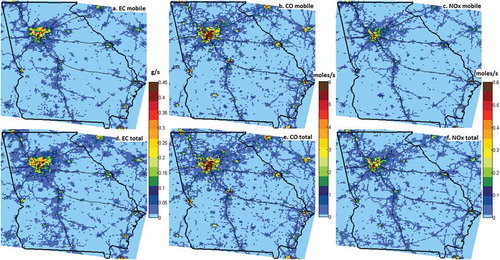
The IMSI method of Pachon et al. (2012) uses county-level National Emissions Inventory (NEI) data. Here, we used simulated annual average emissions (E in eqs 4–6) of the three species as described below at 4 km and 12 km resolutions averaged over time from the HiRes Air Quality Forecasting program (Hu 2014) to match the spatial resolution of the data fusion concentration estimates. These emission estimates were developed using the Sparse Matrix Operator Kernel Emissions Modeling System (SMOKE) (Houyoux et al. 2000) (Figure 2). The emissions of diesel and gasoline vehicles separately were estimated at 36 km resolution and downscaled the ratios of gasoline/diesel to total emissions from 36 km to 4 km using the gasoline/diesel-to-total mobile emission ratio at 36 km resolution and mobile-to-total emission ratio at 4 km resolution as described in the supplemental material (eq S1 and Figure S1). As traffic patterns changed very little over the study period, these weighting factors based on emissions were not varied over time. The temporal variation, such as by day-of-week, season, and year, in the weighting factors was found to be small compared with spatial variation. Mobile source emissions at protected natural resource areas, such as in the Okefenokee Swamp in the southeast corner of Georgia, are very low and highly uncertain. Therefore, we excluded emissions and concentration data in protected natural resource areas (e.g., wilderness areas and national parks) in this study, as our aim was to develop pollutant concentration metrics for health studies. The CMAQ results are based on daily emissions, whereas the IMSI uses annually-averaged annual average level. The spatial distributions of the two emissions are very similar, and the data assimilation technique, along with the IMSI based on observations, addresses the daily variations.

Figure 2. Spatial distributions of annual average emissions at 4 km resolution for mobile sources and total emissions.

CMB source apportionment

The source impacts cannot be measured directly. Mobile source impacts generated by the observation-based receptor model CMB are found to agree well with the long-term trends of NEI (Zhai et al. 2017). In this method, we used the CMB-estimated mobile source impacts as representative of mobile source impacts. We calibrated the unitless indicators to CMB estimates and compared temporal variations of the generated source impacts with CMB estimates at each location.

CMB estimates the source impacts of PM_2.5 by solving mass conservation equations that fit species concentrations to different contributions of various sources (Watson, Cooper, and Huntzicker 1984). To apportion the source impacts, tracer species concentrations are needed. In the Georgia domain, PM_2.5 species concentrations are monitored at 11 sites (Figure S2) from the IMPROVE, SEARCH, and CSN networks from 2002 to 2011 (Hansen et al. 2003; Solomon et al. 2014). The species used in this study include five major species (sulfate, nitrate, ammonium, elemental carbon, and organic carbon) and 14 trace metals that are typically above detection limit (Al, Br, Ca, Cu, Fe, K, Mn, Pb, Sb, Se, Si, Sn, Ti, and Zn). The source profiles summarized by Marmur et al. (2005) for nine sources were used: light-duty gasoline vehicle, heavy-duty diesel vehicle, biomass burning, coal combustion, suspended dust, ammonium sulfate, ammonium bisulfate, ammonium nitrate, and unapportioned organic carbon. The profiles for light-duty gasoline vehicle and heavy-duty diesel vehicle were generated by Chow et al. (2004). More information about the CMB estimates can be found in Zhai et al. (2017).

Spatial PM_2.5 mobile source impact modeling approach

Daily IMSI fields are derived using a single standard deviation for all years and all locations to normalize the indicator species concentrations (see eqs 1–3). The unitless IMSI has the same spatial distribution as the weighted spatial distribution of the indicator species (see Figure 1). To convert the unitless IMSI to a source impact concentration, we perform a power fit regression between the annual average spatial IMSI ($\overline{\mathrm{I}\mathrm{M}\mathrm{S}\mathrm{I}}$) and the annual average CMB results at monitor locations. Using this regression, we can generate the spatial distribution of annual average source impacts at each grid cell (x, y), $\overline{{\mathrm{S}\mathrm{I}}_{xy}}$. Daily source impact fields (SI_x,_y(t)) are then generated using eq 7 by using the spatial distribution of annual average source impacts $\overline{{\mathrm{S}\mathrm{I}}_{xy}}$. To evaluate the impact of the normalization method of the concentrations, we performed an alternative approach, which uses local standard deviation at each location and uses PM_2.5 emissions to estimate the CMB annual averages. More details about the alternative local IMSI method can be found in the supplemental material (Figures S3–S4).

(7) $S{I}_{x,y}\left(t\right)=\frac{IMS{I}_{x,y}\left(t\right)}{\overline{IMS{I}_{x,y}}}\times \overline{S{I}_{x,y}}$(7)

Evaluation

We evaluated the performance of this global IMSI method to predict daily CMB estimates by comparing the IMSI-estimated daily source impacts with the daily CMB estimates at receptor locations using the Pearson correlation coefficient (R), normalized mean bias (NMB) (eq 8), and normalized root mean square error (NRMSE) (eq 9). In the equations, the estimated IMSI source impacts are referred as estimate and the observational-based CMB estimates are referred as OBS. For each site (m), the daily bias (i.e., ${\mathrm{E}\mathrm{s}\mathrm{t}\mathrm{i}\mathrm{m}\mathrm{a}\mathrm{t}\mathrm{e}}_{m,y,d}-{\mathrm{O}\mathrm{B}\mathrm{S}}_{m,y,d})$is normalized by annual averages of observation ($\overline{{\mathrm{O}\mathrm{B}\mathrm{S}}_{m,y}}$) and then averaged through all days (d) and then all years (y). The averaged normalized mean biases at all sites are then averaged for M sites to get a spatiotemporal NMB. Similarly, the root mean square error is calculated using annual averages of daily squared errors (i.e., $({\mathrm{E}\mathrm{s}\mathrm{t}\mathrm{i}\mathrm{m}\mathrm{a}\mathrm{t}\mathrm{e}}_{m,y,d}-{\mathrm{O}\mathrm{B}\mathrm{S}}_{m,y,d}{)}^2)$, then normalized by the annual mean of observation ($\overline{{\mathrm{O}\mathrm{B}\mathrm{S}}_{m,y}}$), and finally averaged across N years and M monitors. Note that only annual average CMB estimates were used in calibration. The temporal trends of CMB estimates and IMSI results are independent and can be used for evaluation.

(8) $NMB=\frac{1}{M}\sum _{m=1}^M\left(\frac{1}{N}\sum _{y=1}^N\frac{1}{D}\sum _{d=1}^D\left(\frac{\left({\mathrm{E}\mathrm{s}\mathrm{t}\mathrm{i}\mathrm{m}\mathrm{a}\mathrm{t}\mathrm{e}}_{m,y,d}-{\mathrm{O}\mathrm{B}\mathrm{S}}_{m,y,d}\right)}{\overline{{\mathrm{O}\mathrm{B}\mathrm{S}}_{m,y}}}\right)\right)$(8)

(9) $NRMSE=\frac{1}{M}\sum _{m=1}^M\left(\frac{1}{N}\sum _{y=1}^N\frac{\sqrt{\frac{1}{D}{\sum }_{d=1}^D{(\mathrm{E}\mathrm{s}\mathrm{t}\mathrm{i}\mathrm{m}\mathrm{a}\mathrm{t}{\mathrm{e}}_{m,y,d}-\mathrm{O}\mathrm{B}{\mathrm{S}}_{m,y,d})}^2}}{\overline{\mathrm{O}\mathrm{B}{\mathrm{S}}_{m,y}}}\right)$(9)

Results and discussion

Results are presented below on the intermediate steps used to derive source impacts, namely, emission-based weighting factors (eqs 4–6) for averaging pollutant indicators and annual average CMB source impact fields for calibrating the IMSI, the spatial and temporal distributions of IMSI source impacts, an evaluation of IMSI source impact estimate performance, and a comparison with an alternative IMSI calibration methodology.

IMSI weighting factors

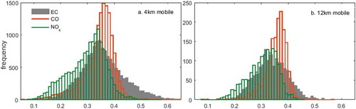
IMSI weighting factors (defined by eqs 4–6) are described in Tables S1 and Figure S5. As shown in Figure 1, CO contributes the most in north Georgia and Atlanta urban areas and EC contributes the most in the southern rural areas. NO_x has an intermediate-level impact in the northern region and lower impact in the southern region. This is due, in part, to the larger contribution of light-duty vehicles emitting CO in the northern urban areas, whereas in the southern rural areas there are more heavy-duty vehicles emitting EC (and NO_x). This results in the IMSI indicators showing similar spatial distribution to CO in the north Georgia and Atlanta urban areas, whereas in the southern areas the spatial distribution of the IMSI indicators is similar to that of EC.

In this application of the IMSI method, the contributions of EC, CO, and NO_x concentrations to the variation of the unitless indicators are substantially different at different locations (Figure 3). The distributions of the weighting factors at 4 km and 12 km are similar, and below we use the 4 km set for discussion. The 2.5%–97.5% quantile range of coefficients at 4 km resolution is 0.21–0.54 for EC, 0.19–0.43 for CO, and 0.15–0.42 for NO_x (Table S1). The weighting factor ranges of CO distributions for mobile indicator are narrower (Figure 3) than the other species. This is because at most locations, CO emissions are largely from mobile sources whereas EC and NO_x have large contributions from other sources, such as power plants for NO_x and rail yards and shipping ports for EC. For DV and GV, EC and CO, respectively, are the major contributing species (Table S1). For example, there is a significant difference in the coefficients across three cities: Atlanta and Denver have similar coefficients, whereas EC coefficients at Houston (Oakes et al. 2014b) are smaller for mobile and DV indicators (Table S2) because of the EC emissions of ships in Houston. This demonstrates the importance of spatial variation caused by local sources and why we should use more spatially resolved weighting factors than county- or city-level factors.

Figure 3. Distribution of weighting factors (eqs 4–6) at all grid cells in Georgia domain at 4 km and 12 km resolutions for mobile sources using annual average emissions.

Spatial CMB annual averages

The IMSI indicators are normalized and unitless, providing information on the daily variation of source impacts but not on the annual average spatial variation of source impacts. We converted the indicators to PM_2.5 mobile source impacts using the power fit regression equation coefficients of annual averages of the IMSI indicators to CMB annual averages, as shown in Table 1 for all years. The IMSI annual averages correlate well with CMB annual averages over space. The correlation is better for total mobile sources than for gasoline and diesel sources. As only annual averages of CMB source impacts are used in the calibration, the daily variations of the CMB results can be used for evaluation.

Table 1. Power fit regression (y = ax^b, where y = CMB and x = IMSI) coefficients for calibrating annual average indicators to annual average CMB source impacts.

		Total mobile			GV			DV
Resolution	Year	a	b	R^2	a	b	R^2	a	b	R^2
12 km	2002	0.44	0.83	0.90	0.25	0.89	0.67	0.13	1.28	0.79
	2003	0.56	0.73	0.90	0.39	0.58	0.37	0.28	0.98	0.78
	2004	0.60	0.79	0.82	0.44	0.62	0.45	0.28	0.98	0.62
	2005	0.61	0.79	0.86	0.39	0.72	0.43	0.28	1.12	0.72
	2006	0.67	0.79	0.89	0.45	0.62	0.45	0.32	1.02	0.72
	2007	0.57	0.76	0.81	0.41	0.51	0.42	0.25	1.11	0.44
	2008	0.72	0.59	0.81	0.36	0.80	0.45	0.28	0.89	0.45
4 km	2008	0.78	0.48	0.75	0.40	0.46	0.65	0.26	0.88	0.72
	2009	0.68	0.58	0.69	0.39	0.47	0.72	0.31	0.49	0.45
	2010	0.82	0.62	0.82	0.46	0.49	0.77	0.34	0.73	0.69

Notes. The coefficients (a, b, and R²) are calculated using the linear regression of log-transformed data.

Spatial PM_2.5 mobile source impacts

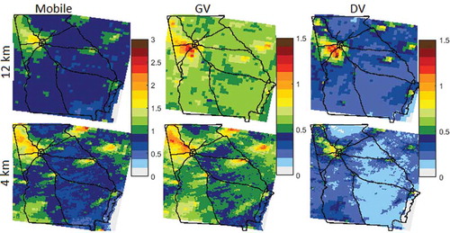
Source impact fields are generated for 2557 days from 2002 to 2008 at 12 km resolution and 1096 days from 2008 to 2010 at 4 km resolution for total mobile sources, gasoline vehicles, and diesel vehicles. As an example, we present spatial distributions of the results on January 21, 2008, in Figure 4 when data for both resolutions are available. The source impacts at the two resolutions show similar urban peaks and downwind peaks from the highways. Differences in the plume direction are observed due to differences in the input wind direction and emissions in the 4 km and 12 km CMAQ simulations. However, the maxima of the 12 km resolution source impacts are substantially lower (maximum of 1.74 µg/m³ for total mobile sources, 1.33 µg/m³ for GV, and 1.75 µg/m³ for DV on this date) compared with the 4 km fields (2.94 µg/m³ for total mobile, 1.71 µg/m³ for GV, and 3.96 µg/m³ for DV). In the rural area, the 12 km estimates higher impact than the 4 km fields, likely due to the spatial smoothing at the 12 km resolution. The GV source impacts are subject to less urban-to-rural difference compared with DV source impacts, which is consistent with the CMB estimates.

Figure 4. Daily source impact (µg/m³) spatial distribution on January 21, 2008, at 12 km and 4 km resolutions for mobile source, GV, and DV.

Temporal trends

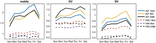
Temporally, the estimated source impacts capture the expected day-of-week trends, with higher impacts on weekdays than weekends because of more traffic on weekdays. Compared with the CMB trends, the estimated source impacts have similar day-of-week distributions. These results are consistent with the emission data and the observational data for the three indicator species. As an example, day-of-week trends are shown in Figure 5 at the grid cells where the urban site in Midtown Atlanta (JST site) and the rural site about 70 km west of Midtown Atlanta (YRK site) are located. These two sites serve as representatives of urban and rural areas. The day-of-week trend is stronger at the urban site than at the rural site as expected due to the urban area’s higher traffic density.

Figure 5. Weekly trends of estimated source impacts (µg/m³) in 2008 at JST (solid lines) and YRK (dashed lines) sites for comparison of the source impacts estimated by the global IMSI method and CMB estimates. JST is an urban site in Midtown Atlanta, and YRK is a rural site about 70 km away from Midtown Atlanta.

Evaluation of the IMSI source impacts using daily observation-based estimates

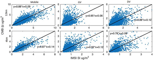
We compared the global IMSI results with daily CMB source impacts at 11 sites to assess performance. Results are shown in Figure 6, and bias, error, and correlation results are listed in Table 2. The estimated total mobile source impacts are well correlated with the CMB estimates (R² = 0.74 and 0.70 for 12 km and 4 km results, respectively), with slope near 1 and intercept near 0. The average bias levels at both resolutions are small, since calibration involves the use of the observation-based annual averages. NRMSE values from eq 9 are lower, and correlations are higher for total mobile impacts than for DV or GV impacts. This can be caused by the uncertainties in CMB as well as in IMSI in separating GV and DV impacts. The uncertainties in separating GV and DV are caused because both sources use similar tracer species. When their unique tracer species are not available, the model cannot separate the two sources well. In CMB, EC and OC are both used as tracer species for GV and DV. For the days when other tracer species are not available, the impacts of the two sources are separated well. In IMSI, only two species are used as tracers for GV and DV with a common NO_x concentration but three tracers are used for mobile sources. This can lead to some bias in the separation of the two sources as well.

Table 2. Bias (NMB), error (NRMSE), and spatiotemporal correlation (R²) for mobile source, GV, and DV impacts on PM_2.5 in comparison with CMB source impacts using the IMSI method.

Parameter	Resolution	Total mobile	GV	DV
NMB	12 km	0.14	0.012	0.35
	4 km	0.19	0.009	0.35
NRMSE	12 km	0.53	0.71	1.32
	4 km	0.60	0.64	1.05
R^2	12 km 4 km	0.74 0.70	0.24 0.41	0.42 0.47

Figure 6. Daily mobile source impacts estimated by CMB and by the global IMSI method (µg/m³) at all sites and years for total mobile, GV, and DV in 12 km resolution (2002–2008) and 4 km resolution (2008–2010).

The overall spatiotemporal correlations (Pearson correlation R-squared, R²) are given in Table 2. In Table 3, temporal correlations (R) are given for each monitor site. These results show that the extended IMSI method agrees better with CMB estimates in locations with higher populations, likely due to the stronger mobile source indicators when traffic density is larger. This also reflects that the method works better at urban areas where the major source of EC, CO, and NOx is mobile sources. In suburban and rural areas, the impact of other sources, such as biomass burning on EC, can impact the performance of the IMSI approach.

Table 3. Correlations (R) between temporal variations of the daily source impacts estimated by the IMSI method and CMB source impacts.

		Total mobile		GV		DV
City	Population	4 km	12 km	4 km	12 km	4 km	12 km
Atlanta	420,003	0.88	0.91	0.57	0.51	0.84	0.68
Athens	115,452	0.64	0.62	0.39	0.25	0.53	0.45
Columbus	189,885	0.74	0.78	0.59	0.41	0.70	0.55
Macon	91,351	0.73	0.78	0.61	0.44	0.64	0.52
Augusta	195,844	0.76	0.81	0.63	0.60	0.64	0.64
Rome	36,303	0.63	0.42	0.37	0.33	0.47	0.35
Douglas	11,589	0.59	0.62	0.20	0.25	0.80	0.53
Charlton County	12,171	0.68	0.69	0.36	0.42	0.76	0.37
Yorkville	17,526	0.63	0.59	0.45	0.27	0.49	0.29

Comparison with an alternative IMSI method using local indicators

Instead of using a single standard deviation for all years and all locations to normalize the indicator species concentrations (which we here refer to as our global IMSI method), we investigated the use of location-specific standard deviations (local IMSI method). This way, the concentrations are normalized to their local levels and the variations of the generated indicators are representative of the local source impact variations over time. Unlike the integrated indicator developed using the global method, the local IMSI does not provide spatial information. Therefore, to calibrate the indicator to source impacts, the annual average IMSI cannot be used in the local method to spatially resolve annual average CMB data. Instead, we develop the annual average source impact field used to calibrate the IMSI using spatially resolved annual average PM_2.5 emissions; these are shown in Figure S3. The daily source impacts are then calculated, as before, using eq 7. Results of the local IMSI method are summarized in Figures S6–S8 and Tables S3–S4 in the supplemental material. These results are very similar to those of the global IMSI method in the application to Georgia, with the global method performing slightly better in terms of temporal correlation with the daily CMB source impacts. This method weights the three species differently and provides different spatial distributions from the global method. It provides an alternative method for locations where the spatial distributions of the three species are not representative of the spatial distribution of mobile sources.

Limitations

Spatially and temporally resolved air pollutant concentration fields are routinely generated in many studies but such fields for source impacts are not due to lack of developed methods for doing so. Traditional source apportionment methods such as CMB and PMF are limited by the availability of observational speciated data and, therefore, are spatially and temporally sparse. Other source apportionment methods in the chemical transport models are computationally expensive and subject to large uncertainties. This method provides an easy way to generate the mobile source impacts when the concentration fields are readily prepared but the generating of the source impacts are time-consuming. The generated results have higher spatial and temporal resolutions and show similar temporal trends to observational estimates by CMB. The results provide high-resolution information on exposure to mobile sources such as gasoline and diesel vehicles at regional levels and will help researchers undercover the adverse health impact by the mobile vehicles. With more evidence from the exposure studies and the source impact estimates, we can make better recommendation for making policies on mobile source emission controls.

However, this approach has some limitations and uncertainties in mainly two aspects. First, this method performs better at urban areas where mobile sources are the major sources of EC, CO, and NO_x. At rural areas or other areas having other major sources of the three species, the method has higher bias and lower correlation with the observational estimate from CMB. However, the urban areas are more populated; therefore, this method can still generate relatively accurate mobile source impacts for the majority of the population. Second, this approach uses CMB estimates and is potentially subject to uncertainties in the CMB method. At annual average level, the uncertainty can be smaller than the temporal estimate.

Conclusion

We developed an approach to estimate the spatial and temporal source impacts of mobile sources on PM_2.5 using three indicator species: CO, NO_x, and EC. The spatial IMSI approach is computationally efficient to apply, as there is no need to run source apportionment methods in a chemical transport model to obtain spatially resolved source impacts. Publicly available chemical transport model results are used to provide the concentration fields necessary to apply the spatial IMSI method. This approach has been applied for generating daily mobile source impacts in Georgia for total mobile sources and for gasoline and diesel vehicles separately from 2002 to 2010. The generated source impacts can capture reasonable spatial distribution and temporal trends and show good spatial and temporal agreement with observational-based source impacts estimated by CMB. The approach agrees well with CMB estimates for total mobile sources but show lower correlation and larger bias for gasoline and diesel vehicles, likely due to the uncertainty in CMB estimates of separate GV/DV impacts. In addition, the approach shows better agreement with CMB estimates in more populated areas because of less impact from other sources of EC, CO, and NO_x in those areas. Overall, the approach developed in this study can estimate spatially and temporally resolved source impacts on PM_2.5 of total mobile sources as well as separate gasoline and diesel vehicle sources. The results are currently being used to evaluate the long-term and statewide exposure to mobile sources of residents in Georgia.

Acknowledgment

The authors acknowledge the projects that provide the data, including the Georgia Tech HiRes2 Air Quality & Source Impacts Forecasting for Georgia, EPA and CDC PHASE Project, and the ambient air quality monitoring networks: IMPROVE, CSN, and SEARCH networks. They acknowledge Valerie Garcia and K. Wyat Appel for supplying PHASE CMAQ modeling results.

Supplemental data

Supplemental data for this paper can be accessed on the publisher’s website.

Additional information

Funding

This research was supported by the U.S. Environmental Protection Agency (under Assistance Agreement No. EPA834799) and by the National Institute of Environmental Health Sciences of the National Institutes of Health (NIH) (under award number R01-ES027892). It has not been formally reviewed by the EPA or NIH. The views expressed in this document are solely those of the authors and do not necessarily reflect those of the EPA or NIH

Notes on contributors

Xinxin Zhai

Xinxin Zhai received her Ph.D. at the Georgia Institute of Technology.

James A. Mulholland

James Mulholland and 

Mariel D. Friberg

Mariel Friberg received her Ph.D. from the Georgia Institute of Technology and now is a NASA Goddard postdoctoral fellow.

Heather A. Holmes

Heather Holmes was a postdoctoral fellows at Georgia Institute of Technology and is now an assistant professor at the University of Nevada, Reno.

Armistead G. Russell

Armistead Russell are professors at the Georgia Institute of Technology.

Yongtao Hu

Yongtao Hu is a research scientist at Georgia Institute of Technology.

References

- Bates, J. T., A. F. Pennington, X. Zhai, M. D. Friberg, F. Metcalf, L. Darrow, M. Strickland, J. Mulholland, and A. Russell. 2018. Application and evaluation of two model fusion approaches to obtain ambient air pollutant concentrations at a fine spatial resolution (250m) in Atlanta. Environ. Modell. Softw. 109:182–90. doi:10.1016/j.envsoft.2018.06.008.
- Beelen, R., O. Raaschou-Nielsen, M. Stafoggia, Z. J. Andersen, G. Weinmayr, B. Hoffmann, K. Wolf, E. Samoli, P. Fischer, M. Nieuwenhuijsen, et al. 2014. Effects of long-term exposure to air pollution on natural-cause mortality: An analysis of 22 European cohorts within the multicentre ESCAPE project. Lancet 383:785–95. doi:10.1016/S0140-6736(13)62158-3.
- Boothe, V., F. Dimmick, V. Haley, C. Paulu, M. Bekkedal, D. Holland, T. Talbot, A. Smith, M. Werner, and E. Baldridge. 2006. A review of public health air surveillance evaluation project. Epidemiology 17:S450–S451. doi:10.1097/00001648-200611001-01208.
- Brauer, M., G. Freedman, J. Frostad, A. van Donkelaar, R. V. Martin, F. Dentener, R. van Dingenen, K. Estep, H. Amini, J. S. Apte, et al. 2016. Ambient air pollution exposure estimation for the global burden of disease 2013. Environ. Sci. Technol. 50:79–88. doi:10.1021/acs.est.5b03709.
- Brauer, M., C. Lencar, L. Tamburic, M. Koehoorn, P. Demers, and C. Karr. 2008. A cohort study of traffic-related air pollution impacts on birth outcomes. Environ. Health. Perspect. 116:680–86. doi:10.1289/ehp.10952.
- Chen, C. H., C. C. Chan, B. Y. Chen, T. J. Cheng, and Y. L. Guo. 2015. Effects of particulate air pollution and ozone on lung function in non-asthmatic children. Environ. Res. 137:40–48. doi:10.1016/j.envres.2014.11.021.
- Chen, H., M. S. Goldberg, R. T. Burnett, M. Jerrett, A. J. Wheeler, and P. J. Villeneuve. 2013. Long-term exposure to traffic-related air pollution and cardiovascular mortality. Epidemiology 24:35–43. doi:10.1097/EDE.0b013e318276c005.
- Chen, L. C., and M. Lippmann. 2009. Effects of metals within ambient air particulate matter (PM) on human health. Inhal. Toxicol. 21:1–31. doi:10.1080/08958370802105405.
- Chow, J. C., J. G. Watson, H. Kuhns, V. Etyemezian, D. H. Lowenthal, D. Crow, S. D. Kohl, J. P. Engelbrecht, and M. C. Green. 2004. Source profiles for industrial, mobile, and area sources in the big bend regional aerosol visibility and observational study. Chemosphere 54:185–208. doi:10.1016/j.chemosphere.2003.07.004.
- Cohen, A. J., H. R. Anderson, B. Ostro, K. D. Pandey, M. Krzyzanowski, N. Kunzli, K. Gutschmidt, A. Pope, I. Romieu, J. M. Samet, et al. 2005. The global burden of disease due to outdoor air pollution. J. Toxicol. Environ. Health 68:1301–07. doi:10.1080/15287390590936166.
- Delfino, R. J., N. Staimer, D. Gillen, T. Tjoa, C. Sioutas, K. Fung, S. C. George, and M. T. Kleinman. 2006. Personal and ambient air pollution is associated with increased exhaled nitric oxide in children with asthma. Environ. Health Persp. 114:1736–43. doi:10.1289/ehp.9141.
- Dominici, F., R. D. Peng, C. D. Barr, and M. L. Bell. 2010. Protecting human health from air pollution shifting from a single-pollutant to a multipollutant approach. Epidemiology 21:187–94. doi:10.1097/EDE.0b013e3181cc86e8.
- Epa, U. S. E. P. A., 2004. EPA-CMB8.2 Usear’s Manual.
- Friberg, M. D., X. Zhai, H. A. Holmes, H. H. Chang, M. J. Strickland, S. E. Sarnat, P. E. Tolbert, A. G. Russell, and J. A. Mulholland. 2016a. Method for fusing observational data and chemical transport model simulations to estimate spatiotemporally resolved ambient air pollution. Environ. Sci. Technol. 50:3695–705. doi:10.1021/acs.est.5b05134.
- Gehring, U., A. H. Wijga, M. Brauer, P. Fischer, J. C. de Jongste, M. Kerkhof, M. Oldenwening, H. A. Smit, and B. Brunekreef. 2010. Traffic-related air pollution and the development of asthma and allergies during the first 8 years of life. Am J Respir Crit Care Med 181:596–603. doi:10.1164/rccm.200906-0858OC.
- Hansen, D. A., E. S. Edgerton, B. E. Hartsell, J. J. Jansen, N. Kandasamy, G. M. Hidy, and C. L. Blanchard. 2003. The southeastern aerosol research and characterization study: Part 1-overview. J. Air. Waste. Manage. Assoc. 53:1460–71. doi:10.1080/10473289.2003.10466318.
- Hart, J. E., E. Garshick, D. W. Dockery, T. J. Smith, L. Ryan, and F. Laden. 2011. Long-term ambient multipollutant exposures and mortality. Am J Respir Crit Care Med 183:73–78. doi:10.1164/rccm.200912-1903OC.
- Held, T., Q. Ying, M. J. Kleeman, J. J. Schauer, and M. P. Fraser. 2005. A comparison of the UCD/CIT air quality model and the CMB source-receptor model for primary airborne particulate matter. Atmos. Environ. 39:2281–97. doi:10.1016/j.atmosenv.2004.12.034.
- Hidy, G. M., and W. T. Pennell. 2010. Multipollutant Air Quality Management. J. Air. Waste. Manage. Assoc. 60:645–74. doi:10.3155/1047-3289.60.6.645.
- Houyoux, M., J. Vukovich, J. Brandmeyer, C. Seppanen, and A. Holland, 2000. Sparse matrix operator kernel emissions modeling system-SMOKE User manual. Prepared by MCNC-North Carolina Supercomputing Center, Environmental Programs, Research Triangle Park, NC.
- Hu, Y., 2014. HiRes2 air quality & source impacts forecasting for Georgia, https://forecast.ce.gatech.edu/hires_about.php.
- Hu, Y., S. Balachandran, J. E. Pachon, J. Baek, C. Ivey, H. Holmes, M. T. Odman, J. A. Mulholland, and A. G. Russell. 2014. Fine particulate matter source apportionment using a hybrid chemical transport and receptor model approach. Atmos. Chem. Phys. 14:5415–31. doi:10.5194/acp-14-5415-2014.
- Hu, Y., M. E. Chang, A. G. Russell, and M. T. Odman. 2010. Using synoptic classification to evaluate an operational air quality forecasting system in Atlanta. Atmos. Pollut. Res. 1:280–87. doi:10.5094/APR.2010.035.
- Huang, R., X. Zhai, C. E. Ivey, M. D. Friberg, X. Hu, Y. Liu, Q. Di, J. Schwartz, J. A. Mulholland, and A. G. Russell. 2018a. Air pollutant exposure field modeling using air quality model-data fusion methods and comparison with satellite AOD-derived fields: Application over North Carolina, USA. Air Qual. Atmos. Health 11:11–22. doi:10.1007/s11869-017-0511-y.
- Huang, Z., Y. Hu, J. Zheng, X. Zhai, and R. Huang. 2018b. An optimized data fusion method and its application to improve lateral boundary conditions in winter for Pearl River Delta regional PM2. 5 modeling, China. Atmos. Environ. 180:59–68. doi:10.1016/j.atmosenv.2018.02.016.
- Ivey, C. E., H. A. Holmes, Y. T. Hu, J. A. Mulholland, and A. G. Russell. 2015. Development of PM2.5 source impact spatial fields using a hybrid source apportionment air quality model. Geosci. Model. Dev. 8:2153–65. doi:10.5194/gmd-8-2153-2015.
- Johns, D. O., L. W. Stanek, K. Walker, S. Benromdhane, B. Hubbell, M. Ross, R. B. Devlin, D. L. Costa, and D. S. Greenbaum. 2012. Practical advancement of multipollutant scientific and risk assessment approaches for ambient air pollution. Environ. Health Persp. 120:1238–42. doi:10.1289/ehp.1204939.
- Kampa, M., and E. Castanas. 2008. Human health effects of air pollution. Environ. Pollut. 151:362–67. doi:10.1016/j.envpol.2007.06.012.
- Kelly, F. J., and J. C. Fussell. 2012. Size, source and chemical composition as determinants of toxicity attributable to ambient particulate matter. Atmos. Environ. 60:504–26. doi:10.1016/j.atmosenv.2012.06.039.
- Kennedy, C. M., A. F. Pennington, L. A. Darrow, M. Klein, X. Zhai, J. T. Bates, A. G. Russell, C. Hansen, P. E. Tolbert, and M. J. Strickland. 2018. Associations of mobile source air pollution during the first year of life with childhood pneumonia, bronchiolitis, and otitis media. Environ. Epidemiol. 2:e007. doi:10.1097/EE9.0000000000000007.
- Kim, J. Y., R. T. Burnett, L. Neas, G. D. Thurston, J. Schwartz, P. E. Tolbert, B. Brunekreef, M. S. Goldberg, and I. Romieu. 2007. Panel discussion review: Session two - interpretation of observed associations between multiple ambient air pollutants and health effects in epidemiologic analyses. J. Expo. Sci. Environ. Epid. 17:S83–S89. doi:10.1038/sj.jes.7500623.
- Kioumourtzoglou, M. A., J. D. Schwartz, M. G. Weisskopf, S. J. Melly, Y. Wang, F. Dominici, and A. Zanobetti. 2016. Long-term PM2.5 exposure and neurological hospital admissions in the Northeastern United States. Environ. Health. Perspect. 124:23–29. doi:10.1289/ehp.1408973.
- Lee, S., W. Liu, Y. H. Wang, A. G. Russell, and E. S. Edgerton. 2008. Source apportionment of PM2.5: Comparing PMF and CMB results for four ambient monitoriniz sites in the southeastern United States. Atmos. Environ. 42:4126–37. doi:10.1016/j.atmosenv.2008.01.025.
- Lelieveld, J., J. S. Evans, M. Fnais, D. Giannadaki, and A. Pozzer. 2015. The contribution of outdoor air pollution sources to premature mortality on a global scale. Nature 525:367-+. doi:10.1038/nature15371.
- Maciejczyk, P., and L. C. Chen. 2005. Effects of subchronic exposures to concentrated ambient particles (CAPs) in mice: VIII. Source-related daily variations in in vitro responses to CAPs. Inhal. Toxicol. 17:243–53. doi:10.1080/08958370590912914.
- Marmur, A., A. Unal, J. A. Mulholland, and A. G. Russell. 2005. Optimization-based source apportionment of PM2.5 incorporating gas-to-particle ratios. Environ. Sci. Technol. 39:3245–54.
- Mauderly, J. L., and J. C. Chow. 2008. Health effects of organic aerosols. Inhal. Toxicol. 20:257–88. doi:10.1080/08958370701866008.
- Melen, E., F. Nyberg, C. M. Lindgren, N. Berglind, M. Zucchelli, E. Nordling, J. Hallberg, M. Svartengren, R. Morgenstern, J. Kere, et al. 2008. Interactions between glutathione S-transferase P1, tumor necrosis factor, and traffic-related air pollution for development of childhood allergic disease. Environ. Health Persp. 116:1077–84. doi:10.1289/ehp.11117.
- Napelenok, S. L., D. S. Cohan, Y. T. Hu, and A. G. Russell. 2006. Decoupled direct 3D sensitivity analysis for particulate matter (DDM-3D/PM). Atmos. Environ. 40:6112–21. doi:10.1016/j.atmosenv.2006.05.039.
- Nordling, E., N. Berglind, E. Melen, G. Emenius, J. Hallberg, F. Nyberg, G. Pershagen, M. Svartengren, M. Wickman, and T. Bellander. 2008. Traffic-related air pollution and childhood respiratory symptoms, function and allergies. Epidemiology 19:401–08. doi:10.1097/EDE.0b013e31816a1ce3.
- Oakes, M., L. Baxter, and T. C. Long. 2014a. Evaluating the application of multipollutant exposure metrics in air pollution health studies. Environ. Int. 69:90–99. doi:10.1016/j.envint.2014.03.030.
- Oakes, M. M., L. K. Baxter, R. M. Duvall, M. Madden, M. J. Xie, M. P. Hannigan, J. L. Peel, J. E. Pachon, S. Balachandran, A. Russell, et al. 2014b. Comparing multipollutant emissions-based mobile source indicators to other single pollutant and multipollutant indicators in different Urban Areas. Int. J. Environ. Res. Pub. He. 11:11727–52. doi:10.3390/ijerph111111727.
- Paatero, P., and U. Tapper. 1994. Positive matrix factorization: A non‐negative factor model with optimal utilization of error estimates of data values. Environmetrics 5:111–26. doi:10.1002/(ISSN)1099-095X.
- Pachon, J. E., S. Balachandran, Y. T. Hu, J. A. Mulholland, L. A. Darrow, J. A. Sarnat, P. E. Tolbert, and A. G. Russell. 2012. Development of outcome-based, multipollutant mobile source indicators. J. Air. Waste. Manage. Assoc. 62:431–42. doi:10.1080/10473289.2012.656218.
- Pennington, A. F., M. J. Strickland, M. Klein, X. Zhai, J. T. Bates, C. Drews-Botsch, C. Hansen, A. G. Russell, P. E. Tolbert, and L. A. Darrow. 2017. Exposure to mobile source air pollution in early-life and childhood asthma incidence: The Kaiser air pollution and pediatric asthma study. Epidemiology 29 (1):22–30. doi:10.1097/EDE.0000000000000754.
- Pope, C. A., 3rd, M. Ezzati, and D. W. Dockery. 2009. Fine-particulate air pollution and life expectancy in the United States. N. Engl. J. Med. 360:376–86. doi:10.1056/NEJMsa0805646.
- Redman, J. D., H. A. Holmes, S. Balachandran, M. L. Maier, X. Zhai, C. Ivey, K. Digby, J. A. Mulholland, and A. G. Russell. 2016. Development and evaluation of a daily temporal interpolation model for fine particulate matter species concentrations and source apportionment. Atmos. Environ. 140:529–38. doi:10.1016/j.atmosenv.2016.06.014.
- Russell, A., P. Tolbert, L. Henneman, J. Abrams, C. Liu, M. Klein, J. Mulholland, S. E. Sarnat, Y. Hu, H. Chang, et al. 2018. Impacts of regulations on air quality and emergency department visits in the Atlanta metropolitan area, 1999-2013. Boston, MA: Health Effects Institute.
- Sarnat, J. A., A. Marmur, M. Klein, E. Kim, A. G. Russell, S. E. Sarnat, J. A. Mulholland, P. K. Hopke, and P. E. Tolbert. 2008. Fine particle sources and cardiorespiratory morbidity: An application of chemical mass balance and factor analytical source-apportionment methods. Environ. Health Persp. 116:459–66. doi:10.1289/ehp.10873.
- Snyder, M. G., A. Venkatram, D. K. Heist, S. G. Perry, W. B. Petersen, and V. Isakov. 2013. RLINE: A line source dispersion model for near-surface releases. Atmos. Environ. 77:748–56. doi:10.1016/j.atmosenv.2013.05.074.
- Solomon, P. A., D. Crumpler, J. B. Flanagan, R. K. M. Jayanty, E. E. Rickman, and C. E. McDade. 2014. US National PM2.5 chemical speciation monitoring networks-CSN and IMPROVE: Description of networks. J. Air. Waste. Manage. 64:1410–38. doi:10.1080/10962247.2014.956904.
- Sturtz, T. M., B. A. Schichtel, and T. V. Larson. 2014. Coupling chemical transport model source attributions with positive matrix factorization: Application to two IMPROVE Sites impacted by wildfires (vol 48, pg 11389, 2014). Environ. Sci. Technol. 48:13021–13021. doi:10.1021/es504856e.
- Uysal, N., and R. M. Schapira. 2003. Effects of ozone on lung function and lung diseases. Curr. Opin. Pulm. Med. 9:144–50.
- Watson, J. G., J. A. Cooper, and J. J. Huntzicker. 1984. The effective variance weighting for least-squares calculations applied to the mass balance receptor model. Atmos. Environ. 18:1347–55. doi:10.1016/0004-6981(84)90043-X.
- West, J. J., A. Cohen, F. Dentener, B. Brunekreef, T. Zhu, B. Armstrong, M. L. Bell, M. Brauer, G. Carmichael, and D. L. Costa. 2016. What we breathe impacts our health: Improving understanding of the link between air pollution and health. Environ. Sci. Technol. 50 (10):4895–904. doi:10.1021/acs.est.5b03827.
- Zeger, S. L., F. Dominici, A. McDermott, and J. M. Samet. 2008. Mortality in the medicare population and chronic exposure to fine particulate air pollution in Urban Centers (2000-2005). Environ. Health Persp. 116:1614–19. doi:10.1289/ehp.11449.
- Zhai, X., J. A. Mulholland, A. G. Russell, and H. A. Holmes. 2017. Spatial and temporal source apportionment of PM 2.5 in Georgia, 2002 to 2013. Atmos. Environ. 161:112–21. doi:10.1016/j.atmosenv.2017.04.039.
- Zhai, X., A. Russell, P. Sampath, J. Mulholland, B.-U. Kim, Y. Kim, and D. D’Onofrio. 2016. Calibrating R-LINE model results with observational data to develop annual mobile source air pollutant fields at fine spatial resolution: Application in Atlanta. Atmos. Environ. 147:446–57. doi:10.1016/j.atmosenv.2016.10.015.