Climate risk and financial stability: evidence from syndicated lending

Abstract

We study the impact of unexpected climate shocks on banks' individual and systemic risks. Employing climate risk measures developed using the Billion-Dollar Weather and Climate Disasters data from the National Oceanic and Atmospheric Administration (NOAA) and Dealscan syndicated lending data, we find that climate risk exposure acquired through cross-state lending increases banks' individual and systemic risks. We also find that bank profitability helps offset some of the adverse effects of climate risk. Banks reduce lending and increase loan loss reserves after the experience of an unexpected climate shock. The loan-level analysis reveals that the effect of climate risk exposure on bank risks is more pronounced for loans granted for operating and capital expenditures. We contribute to a growing literature on the impact of climate risk on financial stability and the development of robust measures of climate risk for banks.

Keywords:

• Bank lending
• climate change
• climate risk
• financial stability
• systemic risk

JEL Classification::

• G20
• G21
• G30
• G32
• N20

1. Introduction

What we have known simply as ‘climate change’ for the past thirty five years is now a global crisis. According to World Economic Forum (2021), climate action failure, extreme weather conditions, and environmental damage arising from human activities are among the most probable risks that the world will be exposed to over the next decade. Regulators are paying close attention to climate change and its implications for financial stability.¹ Central banks and financial regulators have started to design scenarios for climate stress tests to gauge how vulnerable the financial system is to climate change. Despite the sense of urgency and policy significance of this topic, considerable gaps remain in academic research. A major challenge facing both climate finance researchers and practitioners is the shortage of methodologies that facilitate robust measurement of climate risk and promote a successful assessment of the impact of climate change on financial stability (Bank for International Settlements 2021; Battiston, Dafermos, and Monasterolo 2021). The aim of this paper is to make progress in this matter by developing a method to calibrate climate risk and examine its impact on financial stability.

This paper makes several important contributions to the literature. First, we develop the literature on systemic risk by documenting borrower firms' exposure to climate risk as a source for lender banks' systemic risk contribution. Second, we add to the climate risk literature by proposing a climate risk measure that quantifies the extent to which banks are affected by extreme weather events, such as storms, floods, heat waves, and wildfires. In contrast to climate risk measures that focus on specific types of physical climate risks, such as heat exposure (Pankratz, Bauer, and Derwall 2023), or rises in sea levels (Bernstein, Gustafson, and Lewis 2019; Jiang, Li, and Qian 2020; Nguyen et al. 2022), our measure captures the impact of a comprehensive set of physical climate risks. We believe that this set of measures can create an avenue for future research that seeks to examine the impact of climate change on different aspects of social and economic life. Finally, this paper contributes to the ongoing regulatory efforts to measure climate risks and understand their implications for financial stability, providing support for some recent developments in policy aimed at safeguarding monetary and financial stability against climate risk.

Climate risk would appear to meet the minimal definition of a systemic risk proposed by Benoit et al. (2017), as the risk that many market participants are simultaneously affected by severe losses, which then spread through the system.² In this paper, we exploit a setting where unexpected climate shocks transmit via bank lending and propagate through the system, generating financial contagion and elevated systemic risk once the unexpected exposure is priced. Prior studies have identified three primary channels through which shocks can be transmitted which, in turn, intensify systemic risk. The first channel is direct linkages between banks, which may propagate stress from distressed banks to other creditor banks (Allen and Gale 2000). The second channel is the commonality of asset holdings. Shocks can propagate via fire sales when distressed banks deleverage through selling assets (Shleifer and Vishny 1992, 2011). The final channel relies on information contagion (Chen 1999). When a bank is distressed, investors reassess the risk of other banks that are subject to similar exposures. When solvency risks are high, short-term investors may choose not to roll over their investments but engage in precautionary liquidity hoarding (Acharya and Skeie 2011).

We start with creating a bank-level climate risk measure using the Billion-Dollar Weather and Climate Disasters data from the National Oceanic and Atmospheric Administration (NOAA), in conjunction with syndicated lending data from the Dealscan database maintained by the Loan Pricing Corporation (LPC). We focus on syndicated loans for two main reasons: First, syndicated loans are a large and important source of corporate finance for nonfinancial firms in the US (Sufi 2007). Second, syndicated lending essentially operates as a risk-sharing mechanism, making it interesting to examine the transmission of climate risk exposure from borrower firms to banks within the syndication. Our identification strategy to determine the effect of banks' climate risk exposure on their individual and systemic risks consists of four key elements: (1) using an unexpected climate risk measure that cannot be accurately predetermined, thus presenting an exogenous source of variation in climate change and eliminating endogeneity concerns; (2) focusing on cross-state lending instead of within-state lending to isolate the mechanism through which climate risk exposure is transmitted from borrower firms to lender banks; (3) controlling for the book value of loans (i.e. loans-to-assets ratios) to isolate the incremental effect of syndicated lending; and (4) including borrower-firm fixed effects and loan fixed effects to control for latent constant characteristics of borrowers as well as loan demand around origination, allowing the bank-level climate risk measure to explain the remaining variation in banks' individual and systemic risks.

We find that unexpected climate risk exposure acquired through lending activity increases banks' individual and systemic risks. This effect is both statistically and economically significant: An increase of one standard deviation in the bank-level climate risk measure leads to an increase of 14.7% in the marginal expected shortfall, 1.3% in the long-run marginal expected shortfall, 5.9% in the 5% value at risk, 10.2% in the 1% value at risk, 2.7% in the 5% systemic risk contribution, and 6.1% in the 1% systemic risk contribution. We also find that banks reduce lending and increase loan loss reserves subsequent to the experience of a climate shock, and that more profitable banks are able to offset the risk effects of climate risk exposure. We conduct a thorough set of additional analyzes and find that our results are robust to many different specifications.³

Our paper relates to the prior literature documenting the effects of climate risks on both financial and nonfinancial firms. Firms that are more exposed to extremely high temperatures suffer lower revenues and operating income (Pankratz, Bauer, and Derwall 2023). Climate risk impacts the level and volatility of earnings in publicly listed companies, with firms in countries with higher climate risk holding more long-term debt and cash while paying lower cash dividends (Huang, Kerstein, and Wang 2017). Battiston et al. (2017) examine the propagation of climate policy risk through the financial system, finding that the proportion of banks' loan portfolios exposed to climate-policy-relevant sectors is similar to their level of capital held. A further strand of literature focuses on banks' reactions to climate change, showing that banks started pricing climate policy risk by charging marginally higher loan rates to fossil fuel firms after 2015 (Delis, de Greiff, and Ongena 2019), lender banks impose a higher cost of credit for fossil fuel firms that are subject to stricter climate policies and for firms exposed to greater sea level rise (SLR) risk (Jiang, Li, and Qian 2020), and lenders charge higher interest rates for mortgages on properties exposed to a greater risk of SLR (Nguyen et al. 2022).

The remainder of the paper is organized as follows. Section 2 describes the data and approach employed to measure climate risk. Section 3 presents the empirical design. Section 4 presents the main results. Section 5 reports robustness results. Section 6 concludes.

2. Measuring climate risk

Climate change can pose an impact on financial stability in two forms: physical risks and transition risks.⁴ In this paper, we focus on physical climate risks, which adversely affect banks in two primary ways. First, physical climate risks can directly cause damage to physical assets and accelerate the depreciation of capital assets, for example, through a direct connection with extreme weather events such as floods, storms, or wildfires. Such impact can often be offset as insurance generally covers losses due to unexpected catastrophic events. Second, a more relevant impact arises from the fact that physical climate risks can alter (typically reducing) the outputs achievable with a given level of inputs, resulting in a change in the return on capital assets. Banks' credit risk increases and loan quality declines when borrower firms' ability to repay loans is weakened by climate losses. Dietz et al. (2016) document that the estimated impact of climate change on asset value (i.e. climate value at risk or climate VaR) is economically significant and mostly distributed in the tail. More importantly, it is difficult to model and hedge climate risks given the unexpected nature and the long horizon over which such risks may materialize (Financial Stability Board 2020).

2.1. Data

We use the Billion-Dollar Weather and Climate Disasters Data from the National Centers for Environmental Information (NCEI) database maintained by NOAA to measure the state-level climate risk. We employ extreme weather event data as physical climate risks are mostly driven by severe weather events (Li et al. 2024). The NCEI database reports weather and climate disasters where overall losses equaled or exceeded $1 billion. Climate risk events are classified into seven disaster categories: drought, flooding, freezing, severe storms, tropical cyclones, wildfires, and winter storms. For the 1980–2020 reporting cycle, it reports 290 events with total human deaths of 14,492 and total losses exceeding $1.98 trillion,⁵ corresponding to an average of seven events and 353 deaths per year and a loss of $6.8 billion per event (NOAA 2020). In 2020, total losses amounted to $99.5 billion, which accounts for circa 0.5% of the annual GDP of the US for the same period (i.e. $20.94 trillion).

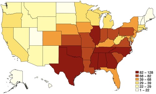
We map the raw climate risk loss data to provide an overview of the variation in climate risk across the states. Figure 1 displays the cumulative losses due to climate risk events during the period of 1980–2020. Figure 2 maps the total number of climate risk events for the same period. Georgia, Mississippi, North Carolina, and Texas are among the high-risk states in terms of both loss severity and frequency over the years.

Figure 1. Cumulative losses (USD bn) of climate risk events 1980–2020.

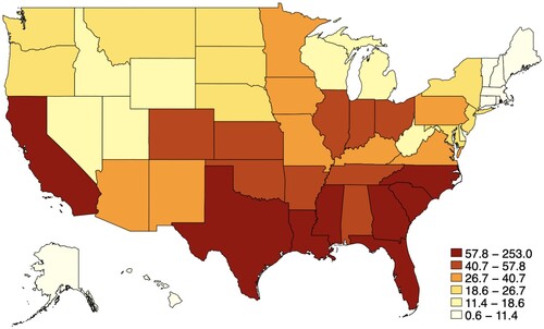
Figure 2. Cumulative frequency of climate risk events 1980–2020.

We collect data on syndicated loans from the Dealscan database maintained by the LPC. Dealscan provides comprehensive information on syndicated loans at origination, including loan amount, maturity, pricing, and identity of lenders and borrowers. A syndicated loan is facilitated by a syndicate of lenders jointly providing funding to a single borrower. The unit of observation in the Dealscan database is a facility (or tranche). A typical syndicated loan deal (or package) consists of multiple facilities initiated at the same time. A deal is arranged by a sole or a few lead lenders who solicit the syndicated members and define the lending arrangement.

We place several restrictions on the Dealscan data to align the climate risk measures with the subsequent analysis requirements. First, we require that the data on the deal value and the date of origination be nonmissing and remove transactions with deal status ‘canceled’, ‘suspended’, or ‘rumour’. Second, since we require information on a bank's allocation share in a loan, we exclude packages with facilities missing information on any lender shares. However, if a package has just one lender and its allocation information is missing, we set the lender share to 100%. Since most loans in Dealscan are syndicated, they are typically associated with one or more lead banks and several participant banks. We retain both lead and participant banks and obtain lender shares for both. Third, we exclude packages with inaccurate lender share information; for instance, when the total of all lender shares exceeds 101%, a threshold that is set to account for minor rounding errors. Lastly, as our focus is on lending made by banks to nonfinancial firms in the United States, we exclude loans made by non-US banks or loans to non-US firms or those in the financial sector (two-digit Standard Industrial Classification (SIC) codes 60–69). Table 1 reports the above sample selection procedure. After four data screening restrictions, we obtain a dataset with 54,642 bank share observations contributed by 571 lender banks and 6,524 borrower firms.

Table 1. Sample selection for climate risk measurement.

	# of lender banks	# of borrower firms	# of bank share observations
Initial Dealscan sample	10,428	73,430	1,747,705
1. Removing deals that are ‘canceled’, ‘suspended’, or ‘rumour’.	10,402	73,074	1,739,874
2. Excluding deals with missing lender share information.	5218	32,272	410,904
3. Excluding deals with inaccurate lender share information.	5164	31,828	396,647
4. Excluding loans made by non-US banks or loans made to non-US firms or financial firms.	571	6524	54,642

This table presents the sample selection procedure undertaken for measuring climate risk.

2.2. Measurement

Our approach to climate risk measurement is largely informed by the methodological framework developed by the Bank for International Settlements (2021), which involves scoring climate risk on the basis of accounting for portfolio and sectoral exposures. The measurement of climate risk comprises two major steps: We first create a state-level climate risk index (CRI_State), and then compute bank-level climate risk exposure (CRI_Bank) by weighting bank lending to a state by the climate risk index of the borrower's state.

CRI_State quantifies the extent to which states have suffered unexpected losses associated with extreme weather events such as storms, floods, and heat waves. CRI_State is indicative of the severity of losses that a state suffers due to climate change, and is based on the following six key climate risk indicators: (1) number of deaths, (2) number of deaths per 100,000 inhabitants, (3) sum of losses in USD at purchasing power parity (PPP), (4) losses per unit of Gross Domestic Product (GDP), (5) number of events, and (6) loss per event. CRI_State is constructed in four steps: First, we perform principal component analysis of these six factors and report the eigenvalues and proportion of the variance explained by the six components in Table 2. As shown in Figure 3, we identify two components with eigenvalues greater than one, explaining 70% of the total variance. Second, we compute the state-level climate risk exposure as the weighted sum of these two significant components, where the weight is given by the eigenvalues. Third, CRI_State is obtained from the residuals from regressing the climate risk exposure of the current year on this variable in the previous three years. CRI_State captures the unexpected variations in climate change, which present credible exogenous shocks as they cannot be accurately predetermined and thus imply that endogeneity issues arising from reverse causality and self selection are unlikely to be a major concern (Auffhammer et al. 2020; Dell, Jones, and Olken 2014; Rao et al. 2022). Finally, we rank CRI_State and scale it by −1 so that a higher score corresponds to greater climate risk for state j in year t.

Figure 3. Scree plot of eigenvalues after PCA.

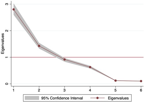
Table 2. Principal component analysis results.

Component	Eigenvalues	Percentage of variance
1	2.802	0.467
2	1.428	0.238
3	0.917	0.153
4	0.630	0.105
5	0.121	0.020
6	0.103	0.017

This table reports the eigenvalues and the proportion of the variance explained by the six components.

The bank-level climate risk is the sum of a bank's lending share to an individual state weighted by the climate risk of the borrower's state, which can be expressed as follows: (1) ${\mathrm{CRI\_Bank}}_{i,t}=\sum \frac{L_{i,j,t}}{T{L}_{i,t}}{\mathrm{CRI\_State}}_{j,t},$(1) where $L_{i,j,t}$ are the total outstanding loans made by bank i to borrowers in state j in year t. $T{L}_{i,t}$ are the total outstanding loans of bank i in year t. $\frac{L_{i,j,t}}{T{L}_{i,t}}$ measures a bank's lending share in state j in year t. $\mathrm{CRI}\mathrm{\_Stat}{e}_{j,t}$ is the climate risk index for state j in year t as defined above. For example, JP Morgan's lending share to borrowers in Texas and Florida is 17% and 6% out of its total syndicated lending in 2016, respectively. We construct two variations of CRI_Bank: CRI_Bank_Cross, and CRI_Bank_Home. The former quantifies unexpected climate risk exposure banks acquire through lending to firms located in a different state (i.e. cross-state lending) while the latter captures unexpected climate risk exposure banks acquire through lending to firms located in the same state (i.e. within-state lending).

3. Empirical design

3.1. Methodology

To examine the impact of bank-level climate risk on financial stability, we exploit the economic link between a lender bank and its borrower firms, and analyze how the exposure of a bank's borrowers to climate risk affects the bank's individual risk and systemic risk contribution. We specify our baseline model as follows: (2) ${\mathrm{Risk}}_{i,t}={\beta }_0+{\beta }_1{\mathrm{CRI\_Bank\_Cross}}_{i,t-1}+\sum _{j=2}^{27}{\beta }_j{\mathrm{Control}}_{i,t-1}+\text{FE}+{ϵ}_{i,t},$(2) where ${\mathrm{Risk}}_{i,t}$ is a set of variables of bank i at time t that is one of the following risk measures: Marginal Expected Shortfall (MES), Long-run Marginal Expected Shortfall (LRMES), VaR5, VaR1, ΔCoVaR5, and ΔCoVaR1.

Following Acharya, Engle, and Richardson (2012), we compute MES as follows: (3) ${\mathrm{MES}}_t^i=E[R_t^i|R_t^m⩽q_{\alpha }],$(3) where $R_t^i$ is the same as previously defined; $R_t^m$ represents the daily financial sector market return at time t; and $q_{\alpha }$ is the α quantile of market returns. Setting α=5%, MES measures the average bank equity return during the 5% worst return days for the banking industry in a year. MES quantifies the extent to which an individual bank's stock returns are low when market returns are low.

LRMES is the long-run marginal expected shortfall (Acharya, Engle, and Richardson 2012), which measures the co-movement of a bank's stock price with the banking industry's market index during its worst 2% return days in a year, and calculated as: (4) ${\mathrm{LRMES}}_t^i=1-\exp (-18\times {\mathrm{MES}}_t^i).$(4) VaR${}_t^i(q)$ focuses on the risk of an individual bank in isolation and is defined as the qth percentile of the potential asset return in percentage $R^i$ that can occur to bank i during a given time period t (Jorion 2006): (5) $P(R^i⩽{\mathrm{VaR}}_t^i(q))=q.$(5) Following Brunnermeier, Dong, and Palia (2020) and Adrian and Brunnermeier (2016), t is set at a weekly interval. Setting q at 5% or 1%, VaR thus measures the worst expected loss of bank i on a weekly basis at either 5% or 1%. The weekly interval is also well-suited for capturing variations in the impact of climate change on stock returns, as the duration of events in our sample ranges from days to months. We then convert weekly VaR to an annual frequency by multiplying the mean weekly VaR during a year by 52.

ΔCoVaR is a statistical measure of tail dependency that does not rely on causality. It captures the direct spillover effects through contractual links, as well as the indirect spillover effects arising from market-wide externalities and the shared exposure of multiple financial institutions to the same risk factors (Adrian and Brunnermeier 2016). Consistent with the approach detailed in Adrian and Brunnermeier (2016), we estimate the time-varying ΔCoVaR for each bank at the 5% and 1% levels. Our estimation is based on quantile regressions using weekly data calculated using CRSP daily stock files for all financial institutions with two-digit Standard Industrial Classification (SIC) code between 60 and 67 inclusive.⁶ We remove daily observations with missing or negative prices and retain banks with nonmissing stock return data on their ordinary common shares for a minimum of 260 weeks. We then merge the weekly stock data with quarterly balance sheet data from the CRSP/Compustat Merged dataset and remove banks with book-to-market and leverage ratios that are less than zero or greater than 100.⁷ The following models are estimated: (6) $\begin{array}{rl}{X}_t^i& ={\alpha }^i+{\gamma }^i{M}_{t-1}+{ϵ}_t^i,\end{array}$(6) (7) $\begin{array}{rl}{X}_t^{\mathrm{system}}& ={\alpha }^{\mathrm{system}|i}+{\beta }^{\mathrm{system}|i}{X}_t^i+{\gamma }^{\mathrm{system}|i}{M}_{t-1}+{ϵ}_t^{\mathrm{system}|i},\end{array}$(7) where X${}_t^i$ is the weekly equity return for bank i at time t; X${}_t^{\mathrm{system}}$ is the weekly return on the market equity of the financial system, calculated as the average market equity weighted by lagged market equity. $M_{t-1}$ is a set of state variables that include the change in the three-month Treasury bill rate, the change in the slope of the yield curve (i.e. the spread between the composite long-term bond yield and three-month Treasury bill rate), a short-term TED spread (i.e. the difference between the three-month LIBOR rate and the three-month Treasury bill rate), the change in credit spread between Moody's seasoned BAA corporate bond yield and the ten-year Treasury rate, the weekly market return computed from the S&P 500 index, the weekly real estate sector return in excess of the financial sector return, and equity volatility calculated as the 22–day rolling standard deviation of the daily CRSP stock market return.

From the estimation of Equations (5(5) $P(R^i⩽{\mathrm{VaR}}_t^i(q))=q.$(5) ) and (6(6) $\begin{array}{rl}{X}_t^i& ={\alpha }^i+{\gamma }^i{M}_{t-1}+{ϵ}_t^i,\end{array}$(6) ) we obtain: (8) $\begin{array}{rl}{\mathrm{VaR}}_t^i(q)& ={\hat{\alpha }}_q^i+{\hat{\gamma }}_q^i{M}_{t-1},\end{array}$(8) (9) $\begin{array}{rl}{\mathrm{CoVaR}}_t^i(q)& ={\hat{\alpha }}_q^{\mathrm{system}|i}+{\hat{\beta }}_q^{\mathrm{system}|i}{\mathrm{VaR}}_t^i(q)+{\hat{\gamma }}_q^{\mathrm{system}|i}{M}_{t-1},\end{array}$(9) where ${\hat{\alpha }}_q^i$, ${\hat{\gamma }}_q^i$, ${\hat{\beta }}_q^{\mathrm{system}|\mathrm{i}}$ and ${\hat{\gamma }}_q^{\mathrm{system}|\mathrm{i}}$ are coefficients obtained from quantile regressions at the 1% and 5% confidence levels. ΔCoVaR${}_t^i(q)$, which measures the marginal contribution of bank i to the risk of the system at time t, is computed as the difference between CoVaR${}_t^i(q)$ conditional on the distress of the institution (i.e. $q=5\mathrm{\%}$ or 1%) and CoVaR${}_t^i(50\mathrm{\%})$ (i.e. the normal state of the institution): (10) $\mathrm{\Delta }{\mathrm{CoVaR}}_t^i(q)={\mathrm{CoVaR}}_t^i(q)-{\mathrm{CoVaR}}_t^i(50\mathrm{\%}).$(10) We obtain weekly ΔCoVaR${}_t^i(q)$ from the quantile regressions and convert it to an annual frequency by first taking the mean of ΔCoVaR${}_t^i(q)$ and then applying a multiplier of 52 for each bank year. We multiply MES, LRMES, VaR5, VaR1, ΔCoVaR5, and ΔCoVaR1 by −1 so that higher values correspond to greater risk.

As discussed in Section 2.2, we create two variations of bank-level climate risk measures: CRI_Bank_Cross and CRI_Bank_Home. The former quantifies unexpected climate risk exposure banks acquire through lending to firms located in a different state (i.e. cross-state lending) while the latter captures unexpected climate risk exposure banks acquire through lending to firms located in the same state (i.e. within-state lending). In our analyzes, the variable of interest is CRI_Bank_Cross because it enables us to pinpoint the mechanism through which climate risk exposure is transmitted from borrower firms to lender banks. This is not the case with CRI_Bank_Home, as it does not facilitate a clear identification of the transmission channel for climate risk. This is because shared climate risk environments among borrower firms and lender banks, when located in the same state, make it difficult to isolate this transmission mechanism. Nevertheless, we include CRI_Bank_Home as an additional control to address concerns about omitted variable bias when not accounting for the effect of within-state lending.

We further control for a set of bank characteristics that are found to be relevant in explaining bank systemic risk (Anginer et al. 2018; Brunnermeier, Dong, and Palia 2020; De Jonghe, Diepstraten, and Schepens 2015; Gauthier, Lehar, and Souissi 2012; Laeven, Ratnovski, and Tong 2016). We include bank size (SIZE_Bank) to control for economies of scale, equity ratio (EQRAT_Bank) to control for bank capital position, market-to-book ratio (MTB_Bank) to control for bank growth opportunities, loans-to-assets ratio (LTA_Bank), loan loss reserves ratio (LLR_Bank) to control for bank loan risk, deposit ratio (DEPO_Bank) to control for bank funding structure, noninterest income ratio (NII_Bank) to control for bank business model, and return on assets (ROA_Bank) to control for bank profitability. Notably, since our CRI_Bank_Cross has an element of bank lending share, controlling for the book value of loans (LTA_Bank) thus allows us to gauge the incremental effect of syndicated lending in addition to bank loan books, on banks' systemic risk. At the borrower firm level, we control for a set of firm characteristics commonly included in debt covenants and relevant for explaining lending decisions and loan quality (Demerjian and Owens 2016), which in turn may affect banks' systemic risk via lending: firm size (SIZE_Borrower), interest coverage (COVER_Borrower), debt-to-EBITDA ratio (DEBT_Borrower), and current ratio (CURRENT_Borrower). We control for GDP per capita and its annual growth rate (ΔGDP) for both lender and borrower states. Variable definitions are detailed in Appendix 1. We also include year fixed effects in all regressions to account for economy-wide shocks on bank risk. We include borrower firm fixed effects to control for latent constant characteristics of each borrower. All continuous independent variables are winsorized at the 1st and 99th percentiles of their empirical distribution.⁸ Standard errors are adjusted for clustering at the bank-borrower lending relationship level.⁹

3.2. Sample and descriptive statistics

We match borrower firms in the Dealscan database with annual financial statement information from Compustat using the linking table provided by Beyhaghi et al. (2021). We use data from the financial year prior to the year of loan origination to ensure that the accounting information is publicly available at the time of loan origination. Using the linking table provided by Schwert (2018), we merge lender banks active in Dealscan with financial statement data from Compustat. We then aggregate all data at lender banks' and borrower firms' parent level to construct the lender-borrower-year sample structure. After applying these two linking tables, the number of lender banks is reduced from 571 to 42¹⁰ and the number of borrower firms decreases from 6,524 to 1,314, resulting in a total of 12,142 lender-borrower-year observations. Table 3 reports composition of the final sample used in our empirical analyzes. Panel A reports sample composition by year. Panel B reports sample composition by lender bank state. Panel C reports sample composition by borrower firm state.

Table 3. Sample composition.

Year	Frequency	Percent	Cumulative
Panel A. Sample Composition by Year
1999	677	5.58	5.58
2000	640	5.27	10.85
2001	691	5.69	16.54
2002	687	5.66	22.20
2003	761	6.27	28.46
2004	807	6.65	35.11
2005	874	7.20	42.31
2006	622	5.12	47.43
2007	555	4.57	52.00
2008	282	2.32	54.32
2009	325	2.68	57.00
2010	722	5.95	62.95
2011	840	6.92	69.86
2012	766	6.31	76.17
2013	602	4.96	81.13
2014	556	4.58	85.71
2015	685	5.64	91.35
2016	492	4.05	95.40
2017	185	1.52	96.93
2018	197	1.62	98.55
2019	176	1.45	100.00
Total	12,142	100.00
State	Frequency	Percent	Cumulative
Panel B. Sample Composition by Lender State
Alabama	271	2.23	2.23
California	1,086	8.94	11.18
Connecticut	38	0.31	11.49
Georgia	836	6.89	18.37
Hawaii	20	0.16	18.54
Illinois	925	7.62	26.16
Louisiana	47	0.39	26.54
Massachusetts	195	1.61	28.15
Minnesota	1,393	11.47	39.62
Mississippi	6	0.05	39.67
New Jersey	23	0.19	39.86
New York	2,206	18.17	58.03
North Carolina	2,167	17.85	75.88
Ohio	1,353	11.14	87.02
Pennsylvania	1,051	8.66	95.68
Rhode Island	25	0.21	95.88
Texas	407	3.35	99.23
Utah	49	0.40	99.64
Wisconsin	44	0.36	100.00
Total	12,142	100.00
Panel C. Sample Composition by Borrower State
Alabama	62	0.51	0.51
Arizona	243	2.00	2.51
Arkansas	98	0.81	3.32
California	592	4.88	8.19
Colorado	237	1.95	10.15
Connecticut	208	1.71	11.86
Delaware	44	0.36	12.22
District of Columbia	107	0.88	13.10
Florida	557	4.59	17.69
Georgia	388	3.20	20.89
Idaho	74	0.61	21.50
Illinois	797	6.56	28.06
Indiana	192	1.58	29.64
Iowa	28	0.23	29.87
Kansas	61	0.50	30.37
Kentucky	205	1.69	32.06
Louisiana	95	0.78	32.84
Maryland	160	1.32	34.16
Massachusetts	304	2.50	36.67
Michigan	459	3.78	40.45
Minnesota	409	3.37	43.81
Mississippi	11	0.09	43.91
Missouri	496	4.08	47.99
Montana	7	0.06	48.05
Nebraska	56	0.46	48.51
Nevada	61	0.50	49.01
New Hampshire	18	0.15	49.16
New Jersey	342	2.82	51.98
New Mexico	12	0.10	52.08
New York	631	5.20	57.27
North Carolina	291	2.40	59.67
North Dakota	12	0.10	59.77
Ohio	761	6.27	66.04
Oklahoma	193	1.59	67.62
Oregon	103	0.85	68.47
Pennsylvania	605	4.98	73.46
Rhode Island	99	0.82	74.27
South Carolina	63	0.52	74.79
South Dakota	33	0.27	75.06
Tennessee	480	3.95	79.01
Texas	1,620	13.34	92.36
Utah	28	0.23	92.59
Vermont	5	0.04	92.63
Virginia	391	3.22	95.85
Washington	170	1.40	97.25
West Virginia	5	0.04	97.29
Wisconsin	329	2.71	100.00
Total	12,142	100.00

This table reports the sample composition. Panel A reports the sample composition by year. Panel B reports the sample composition by lender bank state. Panel C reports the sample composition by borrower firm state.

Table 4 presents descriptive statistics for all variables used in our analysis. For our key dependent variables, the average bank has marginal expected shortfall (−MES) of 3.35%, long-run marginal expected shortfall (−LRMES) of 0.48%, value at risk at the 5% level (−VaR5) of 2.65 %, value at risk at the 1% level (−VaR1) of 4.43%, a systemic risk contribution at the 5% level ($-\mathrm{\Delta }$CoVaR5) of 0.87%, and systemic risk contribution at the 1% level ($-\mathrm{\Delta }$CoVaR1) of 0.78%. For the key independent variable, the average value of CRI_Bank_Cross is −24.30, with a standard deviation of 9.61. CRI_Bank_Cross ranges from −37.16 to 0, with a higher value indicating greater climate risk. Similarly, CRI_Bank_Home has a mean of −26.39 and ranges from −49 to 0. The average bank in our sample has log of total assets (SIZE_Bank) of 12.44 (mean total assets of $560.82 billion), equity ratio (EQRAT_Bank) of 9%, market-to-book ratio (MTB_Bank) of 1.59, deposit ratio (DEPO_Bank) of 63%, loans-to-assets ratio (LTA_Bank) of 51%, nonperforming loans ratio (NPL) of 1%, noninterest income ratio (NII_Bank) of 3%, and return on assets (ROA_Bank) of 1%. These statistics suggest that the average bank tends to be very large and well-capitalized although these averages may mask substantial cross-sectional and time-varying differences. Turning to the borrower controls, we find that the average borrower firm in our sample has a log of total assets (SIZE_Borrower) of 8.08 (mean total assets of $12.41 billion), interest coverage (COVER_Borrower) of 20.29, debt-to-EBITDA ratio (DEBT_Borrower) of 2.44, and current ratio (CURRENT_Borrower) of 0.41. We also note that the average value of log GDP per capita is 10.76 and 10.73 for lender banks' and borrower firms' states, respectively. The average value of annual growth in GDP per capita (ΔGDP) for both lender banks' and borrower firms' states is 3% and 4% for lender banks' and borrower firms' states, respectively.

Table 4. Descriptive statistics.

	N	Mean	S.D.	Min	Median	Max
−MES	12,142	3.35	2.20	0.57	2.97	14.65
−LRMES	12,142	0.48	0.18	0.04	0.48	0.97
−VaR5	12,142	2.65	0.84	1.18	2.47	7.36
−VaR1	12,142	4.43	1.34	2.19	4.11	14.12
$-\mathrm{\Delta }$CoVaR5	12,142	0.87	0.32	0.26	0.84	2.43
$-\mathrm{\Delta }$CoVaR1	12,142	0.78	0.45	0.17	0.70	3.18
CRI_Bank_Cross	12,142	−24.30	9.61	−37.16	−26.79	0.00
CRI_Bank_Home	12,142	−26.39	13.62	−49.00	−28.00	0.00
SIZE_Bank	12,142	12.44	1.29	8.69	12.30	14.67
EQRAT_Bank	12,142	0.09	0.02	0.04	0.09	0.13
MTB_Bank	12,142	1.59	0.76	0.39	1.52	4.11
DEPO_Bank	12,142	0.63	0.10	0.28	0.65	0.86
LTA_Bank	12,142	0.51	0.14	0.12	0.55	0.77
NPL_Bank	12,142	0.01	0.01	0.00	0.00	0.03
NII_Bank	12,142	0.03	0.01	0.01	0.02	0.07
ROA_Bank	12,142	0.01	0.01	−0.01	0.01	0.02
GDP_Bank	12,142	10.76	0.20	10.10	10.75	11.23
ΔGDP_Bank	12,142	0.03	0.02	−0.03	0.04	0.10
SIZE_Borrower	12,142	8.08	1.65	2.56	8.06	11.74
COVER_Borrower	12,142	20.29	41.28	−6.96	8.78	284.68
DEBT_Borrower	12,142	2.44	2.37	−7.04	2.02	16.54
CURRENT_Borrower	12,142	0.41	0.33	0.00	0.33	2.16
GDP_Borrower	12,142	10.73	0.22	10.13	10.71	11.28
ΔGDP_Borrower	12,142	0.04	0.02	−0.03	0.04	0.10

This table presents descriptive statistics of the variables studied. N refers to the number of observations. S.D. is the standard deviation. Min and Max refer to the minimum and maximum values, respectively. Variables are defined in Appendix 1.

4. Results

4.1. Univariate analysis

We report the Pearson correlation between climate risk and banks' individual and systemic risk measures in Panel A of Table 5. All measures for banks' individual and systemic risks are positively correlated at the 1% of statistical significance. CRI_Bank_Cross is positively and significantly correlated with −MES, −LRMES, −VaR5, −VaR1, $-\mathrm{\Delta }$CoVaR5, and $-\mathrm{\Delta }$CoVaR1, which provides preliminary support to our expected relationship about the unexpected climate risk exposure gained through cross-state lending and banks' individual and systemic risks. In Panel B of Table 5, we review the correlation between the climate risk measures and all control variables and find nothing that would indicate issues with multicollinearity.

Table 5. Correlation.

	CRI_Bank_Cross	CRI_Bank_Home	−MES	−LRMES	−VaR5	−VaR1	$-\mathrm{\Delta }$CoVaR5	$-\mathrm{\Delta }$CoVaR1
Panel A. Correlation Between Climate Risk and Systemic Risk Measures
CRI_Bank_Cross	1
CRI_Bank_Home	−0.088${}^{\ast \ast \ast }$	1
−MES	0.102${}^{\ast \ast \ast }$	−0.051${}^{\ast \ast \ast }$	1
−LRMES	0.151${}^{\ast \ast \ast }$	−0.022${}^{\ast }$	0.909${}^{\ast \ast \ast }$	1
−VaR5	0.371${}^{\ast \ast \ast }$	−0.060${}^{\ast \ast \ast }$	0.777${}^{\ast \ast \ast }$	0.741${}^{\ast \ast \ast }$	1
−VaR1	0.278${}^{\ast \ast \ast }$	−0.069${}^{\ast \ast \ast }$	0.710${}^{\ast \ast \ast }$	0.683${}^{\ast \ast \ast }$	0.894${}^{\ast \ast \ast }$	1
$-\mathrm{\Delta }$CoVaR5	0.269${}^{\ast \ast \ast }$	−0.161${}^{\ast \ast \ast }$	0.560${}^{\ast \ast \ast }$	0.558${}^{\ast \ast \ast }$	0.660${}^{\ast \ast \ast }$	0.540${}^{\ast \ast \ast }$	1
$-\mathrm{\Delta }$CoVaR1	0.205${}^{\ast \ast \ast }$	−0.136${}^{\ast \ast \ast }$	0.249${}^{\ast \ast \ast }$	0.285${}^{\ast \ast \ast }$	0.333${}^{\ast \ast \ast }$	0.276${}^{\ast \ast \ast }$	0.780${}^{\ast \ast \ast }$	1
	(1)	(2)	(3)	(4)	(5)	(6)	(7)	(8)	(9)
Panel B. Correlation Between Climate Risk and Control Variables
(1) CRI_Bank_Cross	1
(2) CRI_Bank_Home	−0.088${}^{\ast \ast \ast }$	1
(3) SIZE_Bank	−0.220${}^{\ast \ast \ast }$	0.037${}^{\ast \ast \ast }$	1
(4) EQRAT_Bank	−0.284${}^{\ast \ast \ast }$	0.080${}^{\ast \ast \ast }$	−0.037${}^{\ast \ast \ast }$	1
(5) MTB_Bank	0.400${}^{\ast \ast \ast }$	−0.001	−0.474${}^{\ast \ast \ast }$	−0.362${}^{\ast \ast \ast }$	1
(6) DEPO_Bank	−0.018${}^{\ast }$	0.037${}^{\ast \ast \ast }$	−0.640${}^{\ast \ast \ast }$	0.359${}^{\ast \ast \ast }$	0.160${}^{\ast \ast \ast }$	1
(7) LTA_Bank	0.110${}^{\ast \ast \ast }$	0.056${}^{\ast \ast \ast }$	−0.370${}^{\ast \ast \ast }$	0.237${}^{\ast \ast \ast }$	0.021${}^{\ast }$	0.473${}^{\ast \ast \ast }$	1
(8) NPL_Bank	−0.200${}^{\ast \ast \ast }$	0.002	0.109${}^{\ast \ast \ast }$	0.168${}^{\ast \ast \ast }$	−0.461${}^{\ast \ast \ast }$	0.118${}^{\ast \ast \ast }$	0.314${}^{\ast \ast \ast }$	1
(9) NII_Bank	0.144${}^{\ast \ast \ast }$	−0.037${}^{\ast \ast \ast }$	−0.183${}^{\ast \ast \ast }$	−0.126${}^{\ast \ast \ast }$	0.504${}^{\ast \ast \ast }$	−0.042${}^{\ast \ast \ast }$	−0.412${}^{\ast \ast \ast }$	−0.188${}^{\ast \ast \ast }$	1
(10) ROA_Bank	0.198${}^{\ast \ast \ast }$	0.059${}^{\ast \ast \ast }$	−0.309${}^{\ast \ast \ast }$	0.104${}^{\ast \ast \ast }$	0.616${}^{\ast \ast \ast }$	0.255${}^{\ast \ast \ast }$	0.210${}^{\ast \ast \ast }$	−0.438${}^{\ast \ast \ast }$	0.380${}^{\ast \ast \ast }$
(11) GDP_Bank	−0.404${}^{\ast \ast \ast }$	0.080${}^{\ast \ast \ast }$	0.432${}^{\ast \ast \ast }$	0.241${}^{\ast \ast \ast }$	−0.389${}^{\ast \ast \ast }$	0.029${}^{\ast \ast }$	−0.367${}^{\ast \ast \ast }$	−0.029${}^{\ast \ast }$	−0.105${}^{\ast \ast \ast }$
(12) ΔGDP_Bank	0.057${}^{\ast \ast \ast }$	0.037${}^{\ast \ast \ast }$	−0.076${}^{\ast \ast \ast }$	0.104${}^{\ast \ast \ast }$	0.164${}^{\ast \ast \ast }$	0.059${}^{\ast \ast \ast }$	−0.071${}^{\ast \ast \ast }$	−0.208${}^{\ast \ast \ast }$	0.100${}^{\ast \ast \ast }$
(13) SIZE_Borrower	−0.157${}^{\ast \ast \ast }$	0.027${}^{\ast \ast }$	0.097${}^{\ast \ast \ast }$	0.102${}^{\ast \ast \ast }$	−0.100${}^{\ast \ast \ast }$	0.047${}^{\ast \ast \ast }$	−0.204${}^{\ast \ast \ast }$	−0.013	0.078${}^{\ast \ast \ast }$
(14) COVER_Borrower	−0.013	−0.007	0.036${}^{\ast \ast \ast }$	0.024${}^{\ast \ast }$	−0.037${}^{\ast \ast \ast }$	−0.01	0.002	0.021${}^{\ast }$	−0.032${}^{\ast \ast \ast }$
(15) DEBT_Borrower	0.015	−0.001	0.003	0.018${}^{\ast }$	−0.016	0.011	0.013	0.004	−0.003
(16) CURRENT_Borrower	0.039${}^{\ast \ast \ast }$	−0.009	0.011	−0.018${}^{\ast }$	−0.007	−0.041${}^{\ast \ast \ast }$	0.017	0.040${}^{\ast \ast \ast }$	−0.002
(17) GDP_Borrower	−0.383${}^{\ast \ast \ast }$	0.060${}^{\ast \ast \ast }$	0.289${}^{\ast \ast \ast }$	0.397${}^{\ast \ast \ast }$	−0.464${}^{\ast \ast \ast }$	0.137${}^{\ast \ast \ast }$	−0.082${}^{\ast \ast \ast }$	0.125${}^{\ast \ast \ast }$	−0.189${}^{\ast \ast \ast }$
(18) ΔGDP_Borrower	0.081${}^{\ast \ast \ast }$	−0.054${}^{\ast \ast \ast }$	−0.070${}^{\ast \ast \ast }$	0.030${}^{\ast \ast }$	0.168${}^{\ast \ast \ast }$	−0.037${}^{\ast \ast \ast }$	−0.012	−0.153${}^{\ast \ast \ast }$	0.087${}^{\ast \ast \ast }$
	(10)	(11)	(12)	(13)	(14)	(15)	(16)	(17)	(18)
Panel B. Correlation Between Climate Risk and Control Variables
(1) CRI_Bank_Cross
(2) CRI_Bank_Home
(3) SIZE_Bank
(4) EQRAT_Bank
(5) MTB_Bank
(6) DEPO_Bank
(7) LTA_Bank
(8) NPL_Bank
(9) NII_Bank
(10) ROA_Bank	1
(11) GDP_Bank	−0.120${}^{\ast \ast \ast }$	1
(12) ΔGDP_Bank	0.228${}^{\ast \ast \ast }$	0.078${}^{\ast \ast \ast }$	1
(13) SIZE_Borrower	−0.056${}^{\ast \ast \ast }$	0.286${}^{\ast \ast \ast }$	−0.023${}^{\ast }$	1
(14) COVER_Borrower	−0.014	0.030${}^{\ast \ast \ast }$	0.004	−0.139${}^{\ast \ast \ast }$	1
(15) DEBT_Borrower	−0.013	−0.003	0.005	0.126${}^{\ast \ast \ast }$	−0.307${}^{\ast \ast \ast }$	1
(16) CURRENT_Borrower	−0.016	−0.052${}^{\ast \ast \ast }$	−0.025${}^{\ast \ast }$	−0.083${}^{\ast \ast \ast }$	−0.013	0.050${}^{\ast \ast \ast }$	1
(17) GDP_Borrower	−0.158${}^{\ast \ast \ast }$	0.588${}^{\ast \ast \ast }$	−0.043${}^{\ast \ast \ast }$	0.254${}^{\ast \ast \ast }$	0.058${}^{\ast \ast \ast }$	0.007	−0.057${}^{\ast \ast \ast }$	1
(18) ΔGDP_Borrower	0.197${}^{\ast \ast \ast }$	−0.097${}^{\ast \ast \ast }$	0.467${}^{\ast \ast \ast }$	−0.057${}^{\ast \ast \ast }$	0.003	0.020${}^{\ast }$	−0.045${}^{\ast \ast \ast }$	−0.028${}^{\ast \ast }$	1

Panel A reports Pearson correlation coefficients between climate risk and systemic risk measures. Panel B reports correlation coefficients between climate risk measures and control variables. ${}^{\ast \ast \ast }$, ${}^{\ast \ast }$, and ${}^{\ast }$ indicate statistical significance at the 1%, 5%, and 10% levels, respectively. Variables are defined in Appendix 1.

4.2. The effects of climate risk on banks' individual and systemic risks

Table 6 reports the baseline results from regressions of banks' individual and systemic risks on our climate risk measure and control variables. The variable of interest is CRI_Bank_Cross. We find that ${\beta }_1$, the coefficient for CRI_Bank_Cross, is statistically significant at the 1% level across all model specifications. For the purpose of interpretation, we normalize all variables so that the coefficient captures the effect of a unit (one standard deviation) change in the respective variable on Risk. ${\beta }_1$ thus represents the percentage of additional Risk generated, away from the mean Risk, associated with a one standard deviation increase in the pertinent CRI_Bank_Cross. A unit increase in CRI_Bank_Cross leads to an increase of 14.7% in −MES, 1.3% in −LRMES, 5.9% in −VaR5, 10.2% in −VaR1, 2.7% in $-\mathrm{\Delta }$CoVaR5, and 6.1% in $-\mathrm{\Delta }$CoVaR1. The average variance inflation factor (VIF) of 1.94 indicates that multicollinearity among the regressors should not be a concern. Adjusted $R^2$ ranges from 0.49 to 0.91, suggesting that a substantial proportion of the variation in the dependent variables is explained in the models identified.¹¹

Table 6. The effects of climate risk on banks' individual and systemic risks.

	(1)	(2)	(3)	(4)	(5)	(6)
	−MES	−LRMES	−VaR5	−VaR1	$-\mathrm{\Delta }$CoVaR5	$-\mathrm{\Delta }$CoVaR1
CRI_Bank_Cross	0.147${}^{\ast \ast \ast }$	0.013${}^{\ast \ast \ast }$	0.059${}^{\ast \ast \ast }$	0.102${}^{\ast \ast \ast }$	0.027${}^{\ast \ast \ast }$	0.061${}^{\ast \ast \ast }$
	(7.671)	(7.502)	(6.435)	(4.339)	(5.273)	(6.633)
CRI_Bank_Home	−0.006	0.000	0.007${}^{\ast \ast }$	−0.016${}^{\ast \ast }$	−0.039${}^{\ast \ast \ast }$	−0.035${}^{\ast \ast \ast }$
	(−0.935)	(0.055)	(2.246)	(−2.031)	(−18.777)	(−8.882)
SIZE_Bank	0.087${}^{\ast \ast \ast }$	0.003${}^{\ast \ast }$	0.070${}^{\ast \ast \ast }$	0.154${}^{\ast \ast \ast }$	0.049${}^{\ast \ast \ast }$	−0.049${}^{\ast \ast \ast }$
	(6.094)	(2.122)	(10.051)	(9.295)	(9.962)	(−5.793)
EQRAT_Bank	−0.000	0.003${}^{\ast \ast \ast }$	0.034${}^{\ast \ast \ast }$	0.093${}^{\ast \ast \ast }$	0.025${}^{\ast \ast \ast }$	−0.019${}^{\ast \ast \ast }$
	(−0.006)	(3.922)	(7.360)	(7.672)	(7.084)	(−2.905)
MTB_Bank	0.013	0.009${}^{\ast \ast \ast }$	−0.080${}^{\ast \ast \ast }$	0.012	0.046${}^{\ast \ast \ast }$	0.084${}^{\ast \ast \ast }$
	(0.735)	(6.236)	(−10.024)	(0.593)	(6.840)	(7.429)
DEPO_Bank	−0.077${}^{\ast \ast \ast }$	−0.004${}^{\ast \ast \ast }$	0.033${}^{\ast \ast \ast }$	0.078${}^{\ast \ast \ast }$	0.108${}^{\ast \ast \ast }$	0.212${}^{\ast \ast \ast }$
	(−4.535)	(−2.713)	(4.940)	(4.674)	(22.098)	(24.845)
LTA_Bank	0.048${}^{\ast \ast \ast }$	0.001	−0.150${}^{\ast \ast \ast }$	−0.080${}^{\ast \ast \ast }$	−0.056${}^{\ast \ast \ast }$	−0.126${}^{\ast \ast \ast }$
	(3.322)	(0.517)	(−22.624)	(−4.470)	(−10.872)	(−14.980)
NPL_Bank	0.222${}^{\ast \ast \ast }$	0.023${}^{\ast \ast \ast }$	0.012${}^{\ast }$	−0.034${}^{\ast }$	−0.008${}^{\ast }$	−0.060${}^{\ast \ast \ast }$
	(14.676)	(19.586)	(1.813)	(−1.710)	(−1.904)	(−8.316)
NII_Bank	0.130${}^{\ast \ast \ast }$	0.015${}^{\ast \ast \ast }$	−0.050${}^{\ast \ast \ast }$	−0.086${}^{\ast \ast \ast }$	0.040${}^{\ast \ast \ast }$	0.045${}^{\ast \ast \ast }$
	(11.872)	(13.146)	(−9.558)	(−6.202)	(9.070)	(6.422)
ROA_Bank	−0.267${}^{\ast \ast \ast }$	−0.030${}^{\ast \ast \ast }$	−0.024${}^{\ast \ast \ast }$	−0.041${}^{\ast \ast }$	−0.012${}^{\ast \ast \ast }$	−0.089${}^{\ast \ast \ast }$
	(−19.828)	(−26.157)	(−3.885)	(−2.439)	(−2.891)	(−11.816)
GDP_Bank	−0.169${}^{\ast \ast \ast }$	−0.013${}^{\ast \ast \ast }$	−0.120${}^{\ast \ast \ast }$	−0.420${}^{\ast \ast \ast }$	0.013${}^{\ast \ast \ast }$	−0.057${}^{\ast \ast \ast }$
	(−12.915)	(−11.407)	(−16.047)	(−25.258)	(2.824)	(−6.685)
ΔGDP_Bank	−0.156${}^{\ast \ast \ast }$	−0.004${}^{\ast \ast \ast }$	−0.006	−0.080${}^{\ast \ast \ast }$	−0.004	−0.023${}^{\ast \ast \ast }$
	(−12.997)	(−4.790)	(−1.378)	(−6.758)	(−1.399)	(−4.968)
SIZE_Borrower	0.047	0.005	−0.013	−0.056	0.007	0.012
	(1.221)	(1.361)	(−0.787)	(−1.364)	(0.741)	(0.671)
COVER_Borrower	0.006	−0.000	−0.004	−0.011	0.003	0.007
	(0.470)	(−0.392)	(−0.917)	(−0.833)	(1.079)	(1.453)
DEBT_Borrower	0.008	0.002	0.005	0.015	−0.002	−0.003
	(0.707)	(1.585)	(0.959)	(1.405)	(−0.870)	(−0.642)
CURRENT_Borrower	−0.002	0.001	−0.003	−0.000	0.002	−0.004
	(−0.147)	(0.565)	(−0.484)	(−0.003)	(0.518)	(−0.750)
GDP_Borrower	−0.002	−0.001	0.024	−0.029	0.024${}^{\ast }$	0.049${}^{\ast \ast }$
	(−0.031)	(−0.310)	(1.051)	(−0.487)	(1.766)	(2.084)
ΔGDP_Borrower	−0.007	0.000	0.003	0.009	−0.001	−0.002
	(−0.628)	(0.232)	(0.689)	(0.766)	(−0.520)	(−0.364)
Constant	3.351${}^{\ast \ast \ast }$	0.477${}^{\ast \ast \ast }$	2.653${}^{\ast \ast \ast }$	4.425${}^{\ast \ast \ast }$	0.873${}^{\ast \ast \ast }$	0.778${}^{\ast \ast \ast }$
	(580.371)	(960.696)	(860.958)	(567.684)	(362.269)	(181.959)
Borrower FE	Yes	Yes	Yes	Yes	Yes	Yes
Year FE	Yes	Yes	Yes	Yes	Yes	Yes
Observations	12,142	12,142	12,142	12,142	12,142	12,142
VIF	1.92	1.92	1.92	1.92	1.92	1.92
Adjusted $R^2$	0.914	0.903	0.887	0.712	0.662	0.494

This table reports baseline results of the impact of the banks' climate risk exposure on their individual and systemic risks. The regressions include borrower and year fixed effects (not reported). Standard errors are adjusted for clustering at the bank-borrower (lending relationship) level. ${}^{\ast \ast \ast }$, ${}^{\ast \ast }$ and ${}^{\ast }$ indicate statistical significance at the 1%, 5%, and 10% levels, respectively. Robust t-statistics are reported in parentheses. Variables are defined in Appendix 1.

Many of our bank-specific control variables, chosen to align with the extant literature, are found to be significant. Bank size and equity ratio have a positive and significant association with the risk measures examined, with the exception of $-\mathrm{\Delta }$CoVaR1, where there is a reversal of sign.¹² To try to understand the changes in sign for bank size and equity ratio, two contributing factors must be considered. First, the level of aggregate systemic risk spiked to unprecedented levels following the collapse of Lehman Brothers. Second, subsequent to this event, not all banks were bailed out, and those that were tended to be the very largest and most systemically important ones.¹³ Combining these contributors may explain the changes in sign. During the most significant period of systemic risk, where the focus is on the quantile of most extreme returns, certain banks were more likely to be bailed out. These bailouts, in turn, altered the bank-level systemic risk, as larger, too-big-to-fail banks found themselves in a stronger position, thereby helping to explain the change in sign. The market-to-book ratio, MTB_Bank is positive and significant for the systemic risk measures and negative and significant for −VaR1. The ratio of deposits is negatively related to −MES and −LRMES, and has a positive relationship with the other dependent variables. The positive relationship found for $-\mathrm{\Delta }$CoVaR may relate to its reliance on a series of interest rate variables connected to the attractiveness of deposits. Both loans to assets and nonperforming loans exhibit different relationships with −MES and $-\mathrm{\Delta }$CoVaR in terms of their signs. Net interest income is found to be associated with reduced systemic risk, pointing to the lower risk exposures associated with a traditional loan book. Higher return on assets is linked with a reduction in risk across all measures examined. The GDP and change in GDP of the home state of the bank is associated with a reduction in risk, with the exception of $-\mathrm{\Delta }$CoVaR5, which has a positive sign. This surprising outcome may be linked to possible lags in changes in GDP relative to the more market-based systemic risk. For the extreme changes in systemic risk observed during the global financial crisis, this lag effect might be less evident due to the extended downturn. The only significant effect for the borrower-level variables is in the case of GDP for the $-\mathrm{\Delta }$CoVaR measures.¹⁴

Overall, these results provide evidence that a higher level of unexpected climate risk acquired through cross-state lending leads to greater individual and systemic risks for banks. We next examine the moderating effect of bank profitability on the relationship.

4.3. The moderating role of bank profitability

A large literature considers the relevance of profitability to bank risk-taking, with differing inferences. Early literature conjectures a reduction in risk-taking incentives from higher profitability (Keeley 1990; Repullo 2004). To generate profits, however, banks need to take risks (Blum 1999), and those banks that generate excess profits can build up capital, allowing them to absorb losses (Calem and Rob 1999). Building on this latter notion, Anginer, Demirgüç-Kunt, and Mare (2018) highlight that more capital impacts the risk of individual banks but also a bank's contribution to the risk of the financial system. In light of these arguments, we are investigating whether bank profitability moderates the relationships between climate risk and the systemic risk contribution of banks.

Using an interaction between CRI_Bank_Cross and bank profitability (Profit), we examine the moderating effect of profitability in Table 7. Profit is a dummy variable that is equal to one when a bank's return on assets exceeds the yearly sample median. For −MES and −LRMES, we find no evidence of a moderating impact of bank profitability. For −VaR and $-\mathrm{\Delta }$CoVaR measures, the impact of climate risk is mitigated during periods of higher bank profitability. Assessing the aggregated impact of climate risk along with the interaction, the effect of climate risk is significantly reduced. For example, for $-\mathrm{\Delta }$CoVaR1, the aggregate coefficient is more than halved from 0.117 to 0.052 during times when banks are more profitable. The difference in findings between −MES and $-\mathrm{\Delta }$CoVaR may result from the latter's reliance on state variables, such as interest rates, which affect bank profitability. From a policy perspective, these results highlight the importance of maintaining robust bank profitability as a safeguard against the increasing climate risk to financial stability. Regulators and policymakers should consider bank profitability as a vital factor in enhancing financial system resilience against climate risk.

Table 7. The effects of climate risk on banks' individual and systemic risks: the moderating role of bank profitability.

	(1)	(2)	(3)	(4)	(5)	(6)
	−MES	−LRMES	−VaR5	−VaR1	$-\mathrm{\Delta }$CoVaR5	$-\mathrm{\Delta }$CoVaR1
CRI_Bank_Cross	0.146${}^{\ast \ast \ast }$	0.013${}^{\ast \ast \ast }$	0.117${}^{\ast \ast \ast }$	0.216${}^{\ast \ast \ast }$	0.068${}^{\ast \ast \ast }$	0.117${}^{\ast \ast \ast }$
	(6.298)	(5.667)	(9.417)	(6.942)	(9.279)	(8.692)
Profit	−0.251${}^{\ast \ast \ast }$	−0.022${}^{\ast \ast \ast }$	0.009	0.115${}^{\ast \ast \ast }$	−0.006	0.122${}^{\ast \ast \ast }$
	(−12.785)	(−10.347)	(0.677)	(3.418)	(−0.766)	(9.847)
CRI_Bank_Cross×Profit	0.005	−0.000	−0.065${}^{\ast \ast \ast }$	−0.131${}^{\ast \ast \ast }$	−0.047${}^{\ast \ast \ast }$	−0.065${}^{\ast \ast \ast }$
	(0.282)	(−0.103)	(−6.955)	(−5.995)	(−7.591)	(−5.897)
CRI_Bank_Home	−0.009	−0.000	0.008${}^{\ast \ast }$	−0.013${}^{\ast }$	−0.039${}^{\ast \ast \ast }$	−0.032${}^{\ast \ast \ast }$
	(−1.378)	(−0.354)	(2.561)	(−1.666)	(−18.412)	(−8.328)
Constant	11.446${}^{\ast \ast \ast }$	1.121${}^{\ast \ast \ast }$	7.752${}^{\ast \ast \ast }$	27.218${}^{\ast \ast \ast }$	−2.446${}^{\ast \ast \ast }$	1.249
	(3.828)	(4.715)	(6.521)	(8.908)	(−3.337)	(1.001)
CRI_Bank_Cross+	0.151${}^{\ast \ast \ast }$	0.013${}^{\ast \ast \ast }$	0.052${}^{\ast \ast \ast }$	0.085${}^{\ast \ast \ast }$	0.021${}^{\ast \ast \ast }$	0.052${}^{\ast \ast \ast }$
CRI_Bank_Cross×Profit	(7.750)	(7.640)	(5.600)	(3.650)	(4.110)	(5.530)
Controls	Yes	Yes	Yes	Yes	Yes	Yes
Borrower FE	Yes	Yes	Yes	Yes	Yes	Yes
Year FE	Yes	Yes	Yes	Yes	Yes	Yes
Observations	12,142	12,142	12,142	12,142	12,142	12,142
Adjusted $R^2$	0.915	0.904	0.888	0.713	0.665	0.500

This table reports test results of the moderating role of bank profitability on the impact of climate risk on banks' individual and systemic risks. The regressions include borrower and year fixed effects (not reported). Standard errors are adjusted for clustering at the bank-borrower (lending relationship) level. ${}^{\ast \ast \ast }$ ${}^{\ast \ast }$ and ${}^{\ast }$ indicate statistical significance at the 1%, 5%, and 10% levels, respectively. Robust t-statistics are reported in parentheses. Variables are defined in Appendix 1.

4.4. Business cycle and financial crisis

The nature of systemic risk leads to extended periods of low systemic risk followed by relatively brief states of excessive systemic risk (He and Krishnamurthy 2019). The implication for our work is that the observed positive relationship between climate risk exposure and banks' individual and systemic risks may be influenced by the business cycle. For this reason, we further control for inflation rate to account for the effect of the business cycle. Results, reported in Panel A of Table 8, remain unchanged.

Table 8. The effects of climate risk on banks' individual and systemic risks: business cycle and financial crisis.

	(1)	(2)	(3)	(4)	(5)	(6)
	−MES	−LRMES	−VaR5	−VaR1	$-\mathrm{\Delta }$CoVaR5	$-\mathrm{\Delta }$CoVaR1
Panel A. Controlling for Inflation Rate
CRI_Bank_Cross	0.381${}^{\ast \ast \ast }$	0.043${}^{\ast \ast \ast }$	0.225${}^{\ast \ast \ast }$	0.269${}^{\ast \ast \ast }$	0.057${}^{\ast \ast \ast }$	0.058${}^{\ast \ast \ast }$
	(19.203)	(26.042)	(26.145)	(16.210)	(16.372)	(11.274)
CRI_Bank_Home	−0.034${}^{\ast \ast }$	0.002${}^{\ast }$	0.005	−0.028${}^{\ast \ast \ast }$	−0.040${}^{\ast \ast \ast }$	−0.039${}^{\ast \ast \ast }$
	(−2.480)	(1.919)	(0.863)	(−2.917)	(−15.404)	(−10.311)
Inflation	0.029	0.009${}^{\ast \ast \ast }$	0.172${}^{\ast \ast \ast }$	0.244${}^{\ast \ast \ast }$	0.049${}^{\ast \ast \ast }$	0.042${}^{\ast \ast \ast }$
	(0.944)	(4.777)	(14.444)	(12.670)	(11.757)	(9.194)
Constant	3.351${}^{\ast \ast \ast }$	0.477${}^{\ast \ast \ast }$	2.653${}^{\ast \ast \ast }$	4.425${}^{\ast \ast \ast }$	0.873${}^{\ast \ast \ast }$	0.778${}^{\ast \ast \ast }$
	(337.363)	(619.146)	(595.880)	(495.515)	(332.038)	(179.031)
Controls	Yes	Yes	Yes	Yes	Yes	Yes
Borrower FE	Yes	Yes	Yes	Yes	Yes	Yes
Year FE	No	No	No	No	No	No
Observations	12,142	12,142	12,142	12,142	12,142	12,142
Adjusted $R^2$	0.628	0.635	0.578	0.467	0.454	0.441
Panel B. Interaction Test Results
CRI_Bank_Cross	0.287${}^{\ast \ast \ast }$	0.039${}^{\ast \ast \ast }$	0.183${}^{\ast \ast \ast }$	0.204${}^{\ast \ast \ast }$	0.048${}^{\ast \ast \ast }$	0.053${}^{\ast \ast \ast }$
	(21.473)	(26.205)	(26.572)	(14.318)	(15.230)	(10.732)
Crisis	6.238${}^{\ast \ast \ast }$	0.276${}^{\ast \ast \ast }$	1.829${}^{\ast \ast \ast }$	2.671${}^{\ast \ast \ast }$	0.650${}^{\ast \ast \ast }$	0.425${}^{\ast \ast \ast }$
	(64.068)	(46.814)	(37.646)	(32.176)	(39.371)	(19.064)
CRI_Bank_Cross×Crisis	0.826${}^{\ast \ast \ast }$	0.066${}^{\ast \ast \ast }$	1.657${}^{\ast \ast \ast }$	2.461${}^{\ast \ast \ast }$	0.302${}^{\ast \ast \ast }$	0.213${}^{\ast \ast \ast }$
	(5.801)	(7.125)	(16.749)	(14.584)	(10.276)	(4.832)
CRI_Bank_Home	0.014	0.004${}^{\ast \ast \ast }$	0.009${}^{\ast }$	−0.023${}^{\ast \ast \ast }$	−0.036${}^{\ast \ast \ast }$	−0.037${}^{\ast \ast \ast }$
	(1.499)	(3.850)	(1.911)	(−2.696)	(−15.625)	(−9.931)
Constant	3.040${}^{\ast \ast \ast }$	0.463${}^{\ast \ast \ast }$	2.565${}^{\ast \ast \ast }$	4.296${}^{\ast \ast \ast }$	0.841${}^{\ast \ast \ast }$	0.757${}^{\ast \ast \ast }$
	(423.884)	(612.512)	(636.333)	(501.169)	(336.232)	(170.875)
CRI_Bank_Cross+	1.113${}^{\ast \ast \ast }$	0.105${}^{\ast \ast \ast }$	1.840${}^{\ast \ast \ast }$	2.665${}^{\ast \ast \ast }$	0.350${}^{\ast \ast \ast }$	0.265${}^{\ast \ast \ast }$
CRI_Bank_Cross×Crisis	(7.850)	(11.540)	(18.640)	(15.850)	(12.040)	(6.080)
Controls	Yes	Yes	Yes	Yes	Yes	Yes
Borrower FE	Yes	Yes	Yes	Yes	Yes	Yes
Year FE	No	No	No	No	No	No
Observations	12,142	12,142	12,142	12,142	12,142	12,142
Adjusted $R^2$	0.823	0.694	0.715	0.583	0.553	0.460

This table reports subsample analysis results of business cycle and financial crisis. The regressions include borrower fixed effects (not reported). Standard errors are adjusted for clustering at the bank-borrower (lending relationship) level. ${}^{\ast \ast \ast }$, ${}^{\ast \ast }$ and ${}^{\ast }$ indicate statistical significance at the 1%, 5%, and 10% levels, respectively. Robust t-statistics are reported in parentheses. Variables are defined in Appendix 1.

In addition, during our sample period the global financial crisis (GFC) stands out, with many banks requiring public and private bailouts and a number of financial institutions failing outright. To test the relevance of the GFC to our findings, we interact our variable of interest, CRI_Bank_Cross, with a crisis dummy variable equal to one during the years 2008 and 2009, and zero otherwise. Results are detailed in Panel B of Table 8. For each of the risk measures examined, we find that the baseline findings are consistent: climate risk exposure has a positive and significant relationship with both individual and systemic risks. When considering the combined effect during the crisis period, as indicated by the linear combination of CRI_Bank_Cross and CRI_Bank_Cross×Crisis, we observe an increase in the contribution of climate risk to bank risks during the GFC. Specifically, during the crisis period, there is a substantial increase in the magnitude of the coefficient associated with climate risk. However, this does not necessarily suggest a sizable increase in the influence of climate risk during this period; rather, it reflects a significant increase in bank risk at this time. These findings indicate that climate risk influences banks' individual and systemic risks during both normal and crisis periods.

4.5. The effects of climate risk on banks' subsequent lending behavior

To verify whether unexpected climate risk exposures have a material impact on banks, we perform additional tests to understand the changes in banks' subsequent lending behavior. We employ the following set of outcome variables: the loans-to-asset-ratio (LTA), annual changes in LTA (ΔLTA), the loan loss provision ratio (LLP), and annual changes in LLP (ΔLLP). All independent variables are lagged by one year as we do for the baseline models. Based on the results reported in Table 9, we find that banks reduce lending (Models 1 and 2) and increase loan loss provisions (Models 3 and 4) subsequent to the experience of an unexpected climate shock. These results can be interpreted as either banks adopting more prudent climate risk management after experiencing unexpected climate shocks or climate losses constraining banks' lending capacity. It remains an open empirical question as to whether both effects are at play jointly or whether one is more dominant than the other. This question is out of the scope of the current paper but deserves attention from future research.

Table 9. The effects of climate risk on banks' subsequent lending behavior.

	(1)	(2)	(3)	(4)
	LTA	ΔLTA	LLP	ΔLLP
CRI_Bank_Cross	−0.021${}^{\ast \ast \ast }$	−0.017${}^{\ast \ast \ast }$	0.029${}^{\ast \ast }$	0.903${}^{\ast \ast \ast }$
	(−9.126)	(−7.167)	(1.998)	(5.781)
CRI_Bank_Home	−0.002${}^{\ast \ast \ast }$	−0.006${}^{\ast \ast \ast }$	0.049${}^{\ast \ast \ast }$	−0.162${}^{\ast \ast \ast }$
	(−2.712)	(−6.616)	(10.501)	(−4.707)
SIZE_Bank	−0.022${}^{\ast \ast \ast }$	0.004${}^{\ast \ast }$	0.163${}^{\ast \ast \ast }$	0.176${}^{\ast \ast }$
	(−10.861)	(2.476)	(15.837)	(2.563)
EQRAT_Bank	0.009${}^{\ast \ast \ast }$	0.014${}^{\ast \ast \ast }$	−0.032${}^{\ast \ast \ast }$	−0.176${}^{\ast \ast \ast }$
	(6.243)	(10.133)	(−3.178)	(−3.850)
MTB_Bank	−0.013${}^{\ast \ast \ast }$	0.009${}^{\ast \ast \ast }$	−0.059${}^{\ast \ast \ast }$	0.780${}^{\ast \ast \ast }$
	(−5.673)	(4.336)	(−4.815)	(6.719)
DEPO_Bank	0.026${}^{\ast \ast \ast }$	0.003	−0.086${}^{\ast \ast \ast }$	−0.315${}^{\ast \ast \ast }$
	(12.001)	(1.619)	(−7.743)	(−2.754)
NPL_Bank	0.076${}^{\ast \ast \ast }$	0.008${}^{\ast \ast \ast }$	0.255${}^{\ast \ast \ast }$	0.949${}^{\ast \ast \ast }$
	(47.163)	(6.355)	(22.478)	(8.464)
NII_Bank	−0.080${}^{\ast \ast \ast }$	−0.023${}^{\ast \ast \ast }$	−0.001	−0.988${}^{\ast \ast \ast }$
	(−57.868)	(−20.906)	(−0.139)	(−10.523)
ROA_Bank	0.068${}^{\ast \ast \ast }$	−0.007${}^{\ast \ast \ast }$	0.021${}^{\ast \ast }$	0.099${}^{\ast }$
	(46.198)	(−4.839)	(1.999)	(1.746)
GDP_Bank	−0.041${}^{\ast \ast \ast }$	0.016${}^{\ast \ast \ast }$	−0.003	−0.006
	(−25.253)	(9.933)	(−0.269)	(−0.044)
ΔGDP_Bank	0.002${}^{\ast }$	−0.007${}^{\ast \ast \ast }$	−0.076${}^{\ast \ast \ast }$	0.053
	(1.746)	(−5.649)	(−8.025)	(0.748)
SIZE_Borrower	0.005	−0.000	0.032	0.236
	(1.078)	(−0.121)	(1.133)	(1.317)
COVER_Borrower	0.002	−0.001	−0.003	−0.063
	(1.300)	(−0.373)	(−0.291)	(−0.823)
DEBT_Borrower	0.000	−0.003${}^{\ast }$	0.004	−0.025
	(0.104)	(−1.927)	(0.408)	(−0.437)
CURRENT_Borrower	0.000	−0.002	−0.004	−0.002
	(0.040)	(−1.439)	(−0.426)	(−0.036)
GDP_Borrower	0.005	−0.008	−0.033	−0.068
	(0.780)	(−1.439)	(−0.778)	(−0.214)
ΔGDP_Borrower	0.000	−0.000	0.000	−0.044
	(0.137)	(−0.247)	(0.048)	(−0.642)
Constant	0.501${}^{\ast \ast \ast }$	−0.015${}^{\ast \ast \ast }$	0.853${}^{\ast \ast \ast }$	−0.177${}^{\ast \ast \ast }$
	(624.223)	(−24.276)	(195.247)	(−5.053)
Borrower FE	Yes	Yes	Yes	Yes
Year FE	Yes	Yes	Yes	Yes
Observations	12,103	12,103	12,103	12,103
Adjusted $R^2$	0.769	0.243	0.731	0.070

This table reports test results of the impact of the banks' climate risk exposure on their subsequent lending behavior. The regressions include borrower and year fixed effects (not reported). Standard errors are adjusted for clustering at the bank-borrower (lending relationship) level. ${}^{\ast \ast \ast }$, ${}^{\ast \ast }$ and ${}^{\ast }$ indicate statistical significance at the 1%, 5%, and 10% levels, respectively. Robust t-statistics are reported in parentheses. Variables are defined in Appendix 1.

5. Robustness tests

5.1. Alternative climate risk measures

Extreme weather events may systematically influence stock market performance (Lanfear, Lioui, and Siebert 2019). In order to rule out the possibility that our climate risk measure captures predominantly or acts as a proxy for the systematic effect of climate risk events on the stock market, we create an alternative climate risk measure, CRI_Bank_Res, that is orthogonal to common risk factors identified in prior studies (Bessler and Kurmann 2014; Bessler, Kurmann, and Nohel 2015; Fabrizi, Huan, and Parbonetti 2021), including interest rate risk, credit risk, commodity risk, foreign exchange risk, market risk, political risk, real estate risk, sovereign risk, and the VIX Index. A detailed description of these common risk factors is reported in Appendix 2. CRI_Bank_Cross_Res is computed as the residual from the regression of CRI_Bank_Cross on these common risk factors. We find consistent results based on CRI_Bank_Cross_Res and report them in Panel A of Table 10. The climate risk residual has a consistent and significant positive relationship with bank systemic and individual risks.

Table 10. Alternative climate risk measures.

	(1)	(2)	(3)	(4)	(5)	(6)
	−MES	−LRMES	−VaR5	−VaR1	$-\mathrm{\Delta }$CoVaR5	$-\mathrm{\Delta }$CoVaR1
Panel A. Residual Climate Risk
CRI_Bank_Cross_Res	0.097${}^{\ast \ast \ast }$	0.008${}^{\ast \ast \ast }$	0.040${}^{\ast \ast \ast }$	0.072${}^{\ast \ast \ast }$	0.015${}^{\ast \ast \ast }$	0.039${}^{\ast \ast \ast }$
	(7.816)	(7.355)	(6.760)	(4.698)	(4.547)	(6.649)
CRI_Bank_Home_Res	−0.011	−0.001	0.007${}^{\ast \ast }$	−0.020${}^{\ast \ast }$	−0.043${}^{\ast \ast \ast }$	−0.038${}^{\ast \ast \ast }$
	(−1.630)	(−0.976)	(2.145)	(−2.379)	(−19.837)	(−9.756)
Constant	11.741${}^{\ast \ast \ast }$	1.131${}^{\ast \ast \ast }$	7.622${}^{\ast \ast \ast }$	26.717${}^{\ast \ast \ast }$	−2.382${}^{\ast \ast \ast }$	0.816
	(3.737)	(4.640)	(6.133)	(8.370)	(−3.144)	(0.635)
Borrower FE	Yes	Yes	Yes	Yes	Yes	Yes
Year FE	Yes	Yes	Yes	Yes	Yes	Yes
Observations	11,768	11,768	11,768	11,768	11,768	11,768
Adjusted $R^2$	0.915	0.904	0.887	0.714	0.669	0.502
Panel B. Germanwatch Method
CRI_Bank_Cross_GW	0.019${}^{\ast \ast \ast }$	0.001${}^{\ast \ast \ast }$	0.006${}^{\ast \ast \ast }$	−0.003	0.006${}^{\ast \ast \ast }$	0.011${}^{\ast \ast \ast }$
	(9.364)	(5.818)	(6.097)	(−1.020)	(10.103)	(10.096)
CRI_Bank_Home_GW	−0.028${}^{\ast \ast \ast }$	0.001	−0.000	−0.019${}^{\ast \ast \ast }$	−0.035${}^{\ast \ast \ast }$	−0.024${}^{\ast \ast \ast }$
	(−4.395)	(0.873)	(−0.032)	(−2.663)	(−16.934)	(−6.426)
Constant	12.579${}^{\ast \ast \ast }$	1.204${}^{\ast \ast \ast }$	7.944${}^{\ast \ast \ast }$	27.186${}^{\ast \ast \ast }$	−1.948${}^{\ast \ast \ast }$	1.590
	(4.216)	(5.026)	(6.651)	(8.872)	(−2.666)	(1.278)
Controls	Yes	Yes	Yes	Yes	Yes	Yes
Borrower FE	Yes	Yes	Yes	Yes	Yes	Yes
Year FE	Yes	Yes	Yes	Yes	Yes	Yes
Observations	12,142	12,142	12,142	12,142	12,142	12,142
Adjusted $R^2$	0.915	0.903	0.887	0.711	0.663	0.495

This table reports test results of the impact of the banks' climate risk exposure on their individual and systemic risks based on the use of alternative climate risk measures. Panel A reports results based on an alternative climate risk measure computed as a residual of common risk factors. Panel B reports results using an alternative climate risk measure computed using the Germanwatch method. The regressions include borrower and year fixed effects (not reported). Standard errors are adjusted for clustering at the bank-borrower (lending relationship) level. ${}^{\ast \ast \ast }$, ${}^{\ast \ast }$ and ${}^{\ast }$ indicate statistical significance at the 1%, 5%, and 10% levels, respectively. Robust t-statistics are reported in parentheses. Variables are defined in Appendix 1.

Our main construct for state-level climate risk is based on two principal components of six key climate risk indicators: (1) number of deaths, (2) number of deaths per 100,000 inhabitants, (3) sum of losses in USD at purchasing power parity (PPP), (4) losses per unit of Gross Domestic Product (GDP), (5) number of events, and (6) loss per event. To check the sensitivity of our results to the method of calibrating climate risk, we also apply the Germanwatch method. Each state's climate risk index is the sum of the state's score in the first four indicating categories (i.e. indicators 1 to 4): (11) $\mathrm{CRI\_State\_GW}=\frac{1}{6}\times \mathrm{Death}+\frac{1}{3}\times \frac{\mathrm{Death}}{\mathrm{Population}}+\frac{1}{6}\times \mathrm{Loss}+\frac{1}{3}\times \frac{\mathrm{Loss}}{\mathrm{GDP}}.$(11) We then calculate the bank-level climate risk exposure based on the above Germanwatch state-level climate risk index. Panel B of Table 10 reports results based on this alternative climate risk measure. We find a consistent positive link across all model specifications except for −VaR1, which is found to be insignificant.

5.2. Alternative loan samples

In additional analyzes using alternative loan samples, we first focus on term loans and revolvers because they are the dominant types of loans made by banks to nonfinancial firms in the US (Colla, Ippolito, and Li 2013; Jiang, Li, and Shao 2010; Sufi 2009). A term loan facility entails a loan of a defined sum, with a predetermined repayment schedule and maturity, often fully funded at origination. Revolver facilities usually have shorter maturities compared to term loan facilities and are drawn down at the discretion of the borrower (Lim, Minton, and Weisbach 2014). Following Chu, Zhang, and Zhao (2019), we define a lending observation as a credit line or term loan if it falls within one of the following categories: 364–day facility, revolver/line < 1 year, revolver/line ≥ 1 year, revolver/term loan, term loan, and term loan A. Results, reported in Panel A of Table 11, show a positive and significant link between climate risk and bank systemic and individual risk, highlighting the robustness of our findings to the the choice of loans.

Table 11. Alternative loan samples.

	(1)	(2)	(3)	(4)	(5)	(6)
	−MES	−LRMES	−VaR5	−VaR1	$-\mathrm{\Delta }$CoVaR5	$-\mathrm{\Delta }$CoVaR1
Panel A. Term Loans and Credit Lines Only
CRI_Bank_Cross	0.121${}^{\ast \ast \ast }$	0.010${}^{\ast \ast \ast }$	0.058${}^{\ast \ast \ast }$	0.052${}^{\ast \ast }$	0.031${}^{\ast \ast \ast }$	0.084${}^{\ast \ast \ast }$
	(6.520)	(5.975)	(6.151)	(2.198)	(5.757)	(8.788)
CRI_Bank_Home	−0.009	−0.000	0.004	−0.022${}^{\ast \ast \ast }$	−0.042${}^{\ast \ast \ast }$	−0.037${}^{\ast \ast \ast }$
	(−1.353)	(−0.277)	(1.442)	(−2.812)	(−19.632)	(−9.486)
Constant	12.138${}^{\ast \ast \ast }$	1.144${}^{\ast \ast \ast }$	7.503${}^{\ast \ast \ast }$	25.911${}^{\ast \ast \ast }$	−2.396${}^{\ast \ast \ast }$	1.030
	(3.957)	(4.678)	(6.144)	(8.318)	(−3.234)	(0.823)
Controls	Yes	Yes	Yes	Yes	Yes	Yes
Borrower FE	Yes	Yes	Yes	Yes	Yes	Yes
Year FE	Yes	Yes	Yes	Yes	Yes	Yes
Observations	11,774	11,774	11,774	11,774	11,774	11,774
Adjusted $R^2$	0.914	0.903	0.887	0.713	0.664	0.497
Panel B. Lead Banks Only
CRI_Bank_Cross	0.131${}^{\ast \ast \ast }$	0.015${}^{\ast \ast \ast }$	0.058${}^{\ast \ast }$	0.157${}^{\ast \ast \ast }$	0.029${}^{\ast \ast \ast }$	0.056${}^{\ast \ast \ast }$
	(2.695)	(2.836)	(2.561)	(2.827)	(2.667)	(3.119)
CRI_Bank_Home	0.018	0.002	0.011	−0.002	−0.023${}^{\ast \ast \ast }$	−0.025${}^{\ast \ast }$
	(0.554)	(0.800)	(0.722)	(−0.045)	(−3.315)	(−2.440)
Constant	20.409${}^{\ast }$	1.976${}^{\ast \ast }$	9.747${}^{\ast \ast }$	41.394${}^{\ast \ast \ast }$	4.091${}^{\ast \ast }$	8.065${}^{\ast \ast \ast }$
	(1.925)	(2.508)	(2.510)	(4.294)	(2.390)	(2.905)
Controls	Yes	Yes	Yes	Yes	Yes	Yes
Borrower FE	Yes	Yes	Yes	Yes	Yes	Yes
Year FE	Yes	Yes	Yes	Yes	Yes	Yes
Observations	1,387	1,387	1,387	1,387	1,387	1,387
Adjusted $R^2$	0.947	0.934	0.943	0.848	0.861	0.755

This table presents the test results regarding the impact of banks' climate risk exposure on their individual and systemic risks, using alternative loan samples. Panel A reports results based on a sample of term loans and credit lines. Panel B reports results based on a sample comprising lead banks only. The regressions include borrower and year fixed effects (not reported). Standard errors are adjusted for clustering at the bank-borrower (lending relationship) level. ${}^{\ast \ast \ast }$, ${}^{\ast \ast }$ and ${}^{\ast }$ indicate statistical significance at the 1%, 5%, and 10% levels, respectively. Robust t-statistics are reported in parentheses. Variables are defined in Appendix 1.

To check the robustness of our findings to loan share sales by participating banks, we focus solely on lead banks. Lead banks, also referred to as lead arrangers, originate a loan and then market it to other participant banks (Ivashina and Sun 2011). Lead banks maintain ongoing relationships with borrowers, liaise between borrowers and participant banks, make loan pricing decisions, and bear reputational costs if they misprice loans (Bushman, Williams, and Wittenberg-Moerman 2017; François and Missonier-Piera 2007). For signaling purposes, lead banks tend to retain a larger share in a loan (Sufi 2007). We follow Ivashina (2009) to identify the lead bank(s) of a facility. If a lender is reported as the ‘administrative agent’, we designate it as the lead bank. If no lender is reported as the ‘administrative agent’, we define a lender as the lead bank if it assumes roles of ‘agent’, ‘arranger’, ‘book-runner’, ‘lead arranger’, ‘lead bank’, or ‘lead manager’. As reported in Panel B of Table 11, our main findings remain unchanged using the alternative loan sample of lead banks only.

5.3. Weighted least squares

Panel B of Table 3 indicates a substantial variation in the number of observations across states where lender banks are headquartered. For this reason, we use state-weighted least squares estimation to control for the different weights of lender bank states in the sample. State population is used as the weight. Results for this specification test are reported in Panel A of Table 12. We further employ a capitalization-weighted least squares specification to account for possible greater contributions to systemic risk by larger banks. Laeven, Ratnovski, and Tong (2016) find that larger banks have significantly higher systemic risk contributions. The weight is computed as a bank's end-of-year market capitalization divided by the total capitalization of the financial industry at the same point in time. We report results for this specification in Panel B of Table 12. Results provide further consistent support that climate risk is linked with bank systemic and individual risk.

Table 12. Weighted least squares.

	(1)	(2)	(3)	(4)	(5)	(6)
	−MES	−LRMES	−VaR5	−VaR1	$-\mathrm{\Delta }$CoVaR5	$-\mathrm{\Delta }$CoVaR1
Panel A. Weighted Least Squares (by State Population)
CRI_Bank_Cross	0.147${}^{\ast \ast \ast }$	0.012${}^{\ast \ast \ast }$	0.060${}^{\ast \ast \ast }$	0.103${}^{\ast \ast \ast }$	0.027${}^{\ast \ast \ast }$	0.061${}^{\ast \ast \ast }$
	(7.707)	(7.504)	(6.510)	(4.407)	(5.180)	(6.552)
CRI_Bank_Home	−0.006	0.000	0.007${}^{\ast \ast }$	−0.015${}^{\ast \ast }$	−0.039${}^{\ast \ast \ast }$	−0.035${}^{\ast \ast \ast }$
	(−0.954)	(0.028)	(2.251)	(−2.019)	(−18.755)	(−8.836)
Constant	11.972${}^{\ast \ast \ast }$	1.181${}^{\ast \ast \ast }$	7.825${}^{\ast \ast \ast }$	27.395${}^{\ast \ast \ast }$	−2.357${}^{\ast \ast \ast }$	1.116
	(4.013)	(4.974)	(6.636)	(9.001)	(−3.207)	(0.891)
Controls	Yes	Yes	Yes	Yes	Yes	Yes
Borrower FE	Yes	Yes	Yes	Yes	Yes	Yes
Year FE	Yes	Yes	Yes	Yes	Yes	Yes
Observations	12,142	12,142	12,142	12,142	12,142	12,142
Adjusted $R^2$	0.915	0.903	0.887	0.713	0.663	0.494
Panel B. Weighted Least Squares (by Bank Market Capitalization)
CRI_Bank_Cross	0.149${}^{\ast \ast \ast }$	0.011${}^{\ast \ast \ast }$	0.059${}^{\ast \ast \ast }$	0.099${}^{\ast \ast \ast }$	0.025${}^{\ast \ast \ast }$	0.058${}^{\ast \ast \ast }$
	(7.518)	(7.013)	(6.768)	(4.452)	(4.933)	(6.456)
CRI_Bank_Home	−0.004	0.001${}^{\ast }$	0.005${}^{\ast }$	−0.018${}^{\ast \ast }$	−0.039${}^{\ast \ast \ast }$	−0.032${}^{\ast \ast \ast }$
	(−0.577)	(1.776)	(1.779)	(−2.509)	(−20.627)	(−9.071)
Constant	12.576${}^{\ast \ast \ast }$	1.278${}^{\ast \ast \ast }$	8.779${}^{\ast \ast \ast }$	29.630${}^{\ast \ast \ast }$	−1.704${}^{\ast \ast }$	2.749${}^{\ast \ast }$
	(4.057)	(5.591)	(7.461)	(9.934)	(−2.440)	(2.347)
Controls	Yes	Yes	Yes	Yes	Yes	Yes
Borrower FE	Yes	Yes	Yes	Yes	Yes	Yes
Year FE	Yes	Yes	Yes	Yes	Yes	Yes
Observations	12,142	12,142	12,142	12,142	12,142	12,142
Adjusted $R^2$	0.918	0.910	0.895	0.729	0.678	0.493

This table reports test results of the impact of the banks' climate risk exposure on their individual and systemic risks using Weighted Least Squares (WLS) estimation. Panel A reports results using state population of lender banks as the weight in the estimation. Panel B reports results using banks' market capitalization as the weight in the estimation. The regressions include bank, borrower and year fixed effects (not reported). Standard errors are adjusted for clustering at the bank-borrower (lending relationship) level. ${}^{\ast \ast \ast }$, ${}^{\ast \ast }$ and ${}^{\ast }$ indicate statistical significance at the 1%, 5%, and 10% levels, respectively. Robust t-statistics are reported in parentheses. Variables are defined in Appendix 1.

5.4. Standard errors

We perform three additional tests to check the robustness of our results to the method standard errors are computed. First, we cluster standard errors at borrowers' state level and obtain similar results as reported in Panel A of Table 13. Second, we cluster standard errors at the borrowers' firm level. Our results, reported in Panel B of Table 13, remain unchanged. Lastly, we follow Newey and West (1987) to compute heteroskedasticity- and autocorrelation-consistent (HAC) standard errors that allow for up to two periods of autocorrelation, and report results in Panel B of Table 13. Overall, these results confirm that our main results are robust to different methods of calculating standard errors.

Table 13. Standard errors.

	(1)	(2)	(3)	(4)	(5)	(6)
	−MES	−LRMES	−VaR5	−VaR1	$-\mathrm{\Delta }$CoVaR5	$-\mathrm{\Delta }$CoVaR1
Panel A. Standard Errors Clustered at Borrower State Level
CRI_Bank_Cross	0.147${}^{\ast \ast \ast }$	0.013${}^{\ast \ast \ast }$	0.059${}^{\ast \ast \ast }$	0.102${}^{\ast \ast \ast }$	0.027${}^{\ast \ast \ast }$	0.061${}^{\ast \ast \ast }$
	(7.279)	(5.666)	(5.466)	(4.193)	(4.769)	(6.221)
CRI_Bank_Home	−0.006	0.000	0.007	−0.016	−0.039${}^{\ast \ast \ast }$	−0.035${}^{\ast \ast \ast }$
	(−1.148)	(0.068)	(1.593)	(−1.548)	(−13.416)	(−6.918)
Constant	12.024${}^{\ast \ast \ast }$	1.173${}^{\ast \ast \ast }$	7.819${}^{\ast \ast \ast }$	27.126${}^{\ast \ast \ast }$	−2.370${}^{\ast \ast }$	1.051
	(3.713)	(7.370)	(8.955)	(13.888)	(−2.603)	(0.757)
Controls	Yes	Yes	Yes	Yes	Yes	Yes
Borrower FE	Yes	Yes	Yes	Yes	Yes	Yes
Year FE	Yes	Yes	Yes	Yes	Yes	Yes
Observations	12,142	12,142	12,142	12,142	12,142	12,142
Adjusted $R^2$	0.914	0.903	0.887	0.712	0.662	0.494
Panel B. Standard Errors Clustered at Borrower Firm Level
CRI_Bank_Cross	0.147${}^{\ast \ast \ast }$	0.013${}^{\ast \ast \ast }$	0.059${}^{\ast \ast \ast }$	0.102${}^{\ast \ast \ast }$	0.027${}^{\ast \ast \ast }$	0.061${}^{\ast \ast \ast }$
	(7.219)	(7.732)	(6.688)	(4.442)	(5.623)	(6.832)
CRI_Bank_Home	−0.006	0.000	0.007${}^{\ast \ast }$	−0.016${}^{\ast \ast }$	−0.039${}^{\ast \ast \ast }$	−0.035${}^{\ast \ast \ast }$
	(−0.975)	(0.055)	(2.399)	(−2.116)	(−18.897)	(−8.956)
Constant	12.024${}^{\ast \ast \ast }$	1.173${}^{\ast \ast \ast }$	7.819${}^{\ast \ast \ast }$	27.126${}^{\ast \ast \ast }$	−2.370${}^{\ast \ast \ast }$	1.051
	(4.446)	(6.781)	(8.681)	(12.508)	(−3.589)	(0.983)
Controls	Yes	Yes	Yes	Yes	Yes	Yes
Borrower FE	Yes	Yes	Yes	Yes	Yes	Yes
Year FE	Yes	Yes	Yes	Yes	Yes	Yes
Observations	12,142	12,142	12,142	12,142	12,142	12,142
Adjusted $R^2$	0.914	0.903	0.887	0.712	0.662	0.494
Panel C. Newey-West Standard Errors
CRI_Bank_Cross	0.147${}^{\ast \ast \ast }$	0.013${}^{\ast \ast \ast }$	0.059${}^{\ast \ast \ast }$	0.102${}^{\ast \ast \ast }$	0.027${}^{\ast \ast \ast }$	0.061${}^{\ast \ast \ast }$
	(7.741)	(7.548)	(6.387)	(4.281)	(5.157)	(6.420)
CRI_Bank_Home	−0.006	0.000	0.007${}^{\ast \ast }$	−0.016${}^{\ast \ast }$	−0.039${}^{\ast \ast \ast }$	−0.035${}^{\ast \ast \ast }$
	(−0.936)	(0.056)	(2.284)	(−2.072)	(−19.183)	(−9.435)
Constant	11.885${}^{\ast \ast \ast }$	1.150${}^{\ast \ast \ast }$	8.321${}^{\ast \ast \ast }$	27.096${}^{\ast \ast \ast }$	−2.242${}^{\ast \ast \ast }$	0.941
	(4.300)	(5.128)	(6.837)	(8.706)	(−2.989)	(0.719)
Controls	Yes	Yes	Yes	Yes	Yes	Yes
Borrower FE	Yes	Yes	Yes	Yes	Yes	Yes
Year FE	Yes	Yes	Yes	Yes	Yes	Yes
Observations	12,142	12,142	12,142	12,142	12,142	12,142
Adjusted $R^2$	0.914	0.903	0.887	0.712	0.662	0.494

This table reports test results of the impact of the banks' climate risk exposure on their individual and systemic risks. Panel A reports results with standard errors adjusted for clustering at the borrower state level. Panel B reports results with standard errors adjusted for clustering at the borrower's firm level. Panel C reports results with heteroskedasticity- and autocorrelation-consistent (HAC) standard errors computed following the Newey and West (1987) procedure that allows for up to two periods of autocorrelation. The regressions include bank, borrower and year fixed effects (not reported). ${}^{\ast \ast \ast }$, ${}^{\ast \ast }$ and ${}^{\ast }$ indicate statistical significance at the 1%, 5%, and 10% levels, respectively. Robust t-statistics are reported in parentheses. Variables are defined in Appendix 1.

5.5. Alternative fixed effects specifications

In our baseline model specifications, we include both year and borrower firm fixed effects. We also examine our results using alternative fixed effects specifications. In one specification, we include only the year fixed effect, and in another, we do not include any fixed effects. Results for these two specifications are reported in Panel A and B of Table 14, respectively, and remain consistent with our baseline findings, showing that climate risk is linked with bank systemic and individual risks. Of particular note, the adjusted R-squared is found to decrease substantially when year fixed effects are excluded, suggesting that the high R-squared observed in our baseline models are at least partially a consequence of year fixed effects.

Table 14. Alternative fixed effects specifications.

	(1)	(2)	(3)	(4)	(5)	(6)
	−MES	−LRMES	−VaR5	−VaR1	$-\mathrm{\Delta }$CoVaR5	$-\mathrm{\Delta }$CoVaR1
Panel A. Year Fixed Effects Only
CRI_Bank_Cross	0.147${}^{\ast \ast \ast }$	0.013${}^{\ast \ast \ast }$	0.064${}^{\ast \ast \ast }$	0.111${}^{\ast \ast \ast }$	0.029${}^{\ast \ast \ast }$	0.060${}^{\ast \ast \ast }$
	(8.156)	(8.275)	(6.688)	(4.727)	(5.578)	(6.348)
CRI_Bank_Home	−0.009	−0.001	0.007${}^{\ast \ast }$	−0.015${}^{\ast \ast }$	−0.040${}^{\ast \ast \ast }$	−0.036${}^{\ast \ast \ast }$
	(−1.428)	(−0.903)	(2.337)	(−1.965)	(−19.547)	(−9.301)
Constant	11.225${}^{\ast \ast \ast }$	1.055${}^{\ast \ast \ast }$	9.058${}^{\ast \ast \ast }$	26.288${}^{\ast \ast \ast }$	−1.609${}^{\ast \ast \ast }$	2.493${}^{\ast \ast \ast }$
	(13.317)	(13.996)	(18.211)	(22.889)	(−4.850)	(4.096)
Controls	Yes	Yes	Yes	Yes	Yes	Yes
Borrower FE	No	No	No	No	No	No
Year FE	Yes	Yes	Yes	Yes	Yes	Yes
Observations	12,142	12,142	12,142	12,142	12,142	12,142
Adjusted $R^2$	0.914	0.903	0.883	0.706	0.655	0.484
Panel B. No Fixed Effects
CRI_Bank_Cross	0.352${}^{\ast \ast \ast }$	0.044${}^{\ast \ast \ast }$	0.266${}^{\ast \ast \ast }$	0.296${}^{\ast \ast \ast }$	0.066${}^{\ast \ast \ast }$	0.060${}^{\ast \ast \ast }$
	(24.172)	(36.589)	(40.044)	(23.030)	(22.566)	(13.085)
CRI_Bank_Home	−0.056${}^{\ast \ast \ast }$	0.001	−0.001	−0.040${}^{\ast \ast \ast }$	−0.043${}^{\ast \ast \ast }$	−0.043${}^{\ast \ast \ast }$
	(−3.961)	(1.047)	(−0.229)	(−3.855)	(−16.156)	(−11.419)
Constant	−15.011${}^{\ast \ast \ast }$	−1.259${}^{\ast \ast \ast }$	8.487${}^{\ast \ast \ast }$	15.243${}^{\ast \ast \ast }$	−1.327${}^{\ast \ast \ast }$	0.165
	(−12.109)	(−12.780)	(13.767)	(14.205)	(−5.190)	(0.432)
Controls	Yes	Yes	Yes	Yes	Yes	Yes
Borrower FE	No	No	No	No	No	No
Year FE	No	No	No	No	No	No
Observations	12,142	12,142	12,142	12,142	12,142	12,142
Adjusted $R^2$	0.537	0.552	0.445	0.354	0.361	0.406

This table reports test results of the impact of the banks' climate risk exposure on their individual and systemic risks based on different fixed effects choices. Panel A reports results using state population of lender banks as the weight in the estimation. Panel B reports results using banks' market capitalization as the weight in the estimation. The regressions include bank, borrower and year fixed effects (not reported). Standard errors are adjusted for clustering at the bank-borrower (lending relationship) level. ${}^{\ast \ast \ast }$, ${}^{\ast \ast }$ and ${}^{\ast }$ indicate statistical significance at the 1%, 5%, and 10% levels, respectively. Robust t-statistics are reported in parentheses. Variables are defined in Appendix 1.

5.6. Loan-level analyzes

We perform several additional tests using the loan-level sample to check if our baseline results hold at the deal level. The loan-level sample includes 2,918 deal packages and 3,699 facilities with available bank share information, which correspond to 15,037 bank share observations. We report the main results of the loan-level analysis in Table 15. Panel A, B, and C report results with standard errors clustered at the lending relationship level, the package level, and the facility level, respectively. Results remain consistent with the baseline results under different specifications of standard error clustering.

Table 15. Loan-level analyzes: main results.

	(1)	(2)	(3)	(4)	(5)	(6)
	−MES	−LRMES	−VaR5	−VaR1	$-\mathrm{\Delta }$CoVaR5	$-\mathrm{\Delta }$CoVaR1
Panel A. Standard Errors Clustered at the Lending Relationship Level
CRI_Bank_Cross	0.144${}^{\ast \ast \ast }$	0.013${}^{\ast \ast \ast }$	0.063${}^{\ast \ast \ast }$	0.112${}^{\ast \ast \ast }$	0.028${}^{\ast \ast \ast }$	0.064${}^{\ast \ast \ast }$
	(6.532)	(6.663)	(6.033)	(4.022)	(4.974)	(6.071)
CRI_Bank_Home	−0.007	0.000	0.006${}^{\ast }$	−0.016${}^{\ast }$	−0.042${}^{\ast \ast \ast }$	−0.038${}^{\ast \ast \ast }$
	(−0.972)	(0.032)	(1.885)	(−1.884)	(−18.424)	(−8.968)
Constant	13.569${}^{\ast \ast \ast }$	1.310${}^{\ast \ast \ast }$	7.530${}^{\ast \ast \ast }$	25.517${}^{\ast \ast \ast }$	−2.224${}^{\ast \ast \ast }$	0.746
	(4.373)	(5.044)	(6.145)	(8.205)	(−2.748)	(0.540)
Controls	Yes	Yes	Yes	Yes	Yes	Yes
Borrower FE	Yes	Yes	Yes	Yes	Yes	Yes
Year FE	Yes	Yes	Yes	Yes	Yes	Yes
Observations	15,037	15,037	15,037	15,037	15,037	15,037
Adjusted $R^2$	0.913	0.901	0.889	0.711	0.663	0.497
Panel B. Standard Errors Clustered at the Package Level
CRI_Bank_Cross	0.144${}^{\ast \ast \ast }$	0.013${}^{\ast \ast \ast }$	0.063${}^{\ast \ast \ast }$	0.112${}^{\ast \ast \ast }$	0.028${}^{\ast \ast \ast }$	0.064${}^{\ast \ast \ast }$
	(5.857)	(6.638)	(6.139)	(4.011)	(5.040)	(6.034)
CRI_Bank_Home	−0.007	0.000	0.006${}^{\ast \ast }$	−0.016${}^{\ast \ast }$	−0.042${}^{\ast \ast \ast }$	−0.038${}^{\ast \ast \ast }$
	(−0.962)	(0.031)	(1.964)	(−1.981)	(−18.671)	(−9.707)
Constant	13.569${}^{\ast \ast \ast }$	1.310${}^{\ast \ast \ast }$	7.530${}^{\ast \ast \ast }$	25.517${}^{\ast \ast \ast }$	−2.224${}^{\ast \ast \ast }$	0.746
	(5.835)	(7.642)	(8.102)	(11.526)	(−3.807)	(0.773)
Controls	Yes	Yes	Yes	Yes	Yes	Yes
Borrower FE	Yes	Yes	Yes	Yes	Yes	Yes
Year FE	Yes	Yes	Yes	Yes	Yes	Yes
Observations	15,037	15,037	15,037	15,037	15,037	15,037
Adjusted $R^2$	0.913	0.901	0.889	0.711	0.663	0.497
Panel C. Standard Errors Clustered at the Facility Level
CRI_Bank_Cross	0.144${}^{\ast \ast \ast }$	0.013${}^{\ast \ast \ast }$	0.063${}^{\ast \ast \ast }$	0.112${}^{\ast \ast \ast }$	0.028${}^{\ast \ast \ast }$	0.064${}^{\ast \ast \ast }$
	(6.864)	(8.224)	(7.324)	(5.017)	(5.751)	(7.043)
CRI_Bank_Home	−0.007	0.000	0.006${}^{\ast \ast }$	−0.016${}^{\ast \ast }$	−0.042${}^{\ast \ast \ast }$	−0.038${}^{\ast \ast \ast }$
	(−1.129)	(0.038)	(2.302)	(−2.392)	(−22.194)	(−11.558)
Constant	13.569${}^{\ast \ast \ast }$	1.310${}^{\ast \ast \ast }$	7.530${}^{\ast \ast \ast }$	25.517${}^{\ast \ast \ast }$	−2.224${}^{\ast \ast \ast }$	0.746
	(6.242)	(8.787)	(8.871)	(12.765)	(−4.355)	(0.877)
Controls	Yes	Yes	Yes	Yes	Yes	Yes
Borrower FE	Yes	Yes	Yes	Yes	Yes	Yes
Year FE	Yes	Yes	Yes	Yes	Yes	Yes
Observations	15,037	15,037	15,037	15,037	15,037	15,037
Adjusted $R^2$	0.913	0.901	0.889	0.711	0.663	0.497

This table reports the loan-level analysis results of the impact of the banks' climate risk exposure on their individual and systemic risks. The regressions include borrower and year fixed effects (not reported). ${}^{\ast \ast \ast }$, ${}^{\ast \ast }$ and ${}^{\ast }$ indicate statistical significance at the 1%, 5%, and 10% levels, respectively. Robust t-statistics are reported in parentheses. Variables are defined in Appendix 1.

The loan-level data structure also enables us to exploit the variation across different types of loans categorized by their intended purpose. We classify syndicated loans into three primary categories: (1) Operating and capital expenditures: if a loan is granted for capital expenditures, equipment purchase, real estate, or working capital; (2) Capital structure: if a loan is made for initial public offering, recapitalization, securities purchase, or stock buyback; and (3) M&A and buyouts: if a loan is granted for acquisitions, mergers, takeover, leveraged buyout, management buyout, or secondary buyout. We then create dummy variables based on these categories and interact them with our bank-level climate risk measure. The resulting interaction term captures the moderating role of specific loan purposes on the effects of climate risk on banks' individual and systemic risks. We report the test results in Table 16. We find that the coefficient for the interaction term is significant and positive for loans made for operating and capital expenditures (columns 2, 3, 4, 5, and 6 of Panel A), indicating that the effect of climate risk exposure on bank risks is more pronounced for loans earmarked for operating and capital expenditures. This finding is in line with the underlying premise of this study, which posits that as climate losses weaken borrower firms' ability to repay loans, banks' credit risk increases and loan quality deteriorates. Results for loans granted for capital structure (Panel B) and M&A and buyouts (Panel C) are not significant, except for −MES in column 1 for both tests.

Table 16. Loan-level analyzes: the moderating role of loan purposes

	(1)	(2)	(3)	(4)	(5)	(6)
	−MES	−LRMES	−VaR5	−VaR1	$-\mathrm{\Delta }$CoVaR5	$-\mathrm{\Delta }$CoVaR1
Panel A. Operating and Capital Expenditure
CRI_Bank_Cross	0.140${}^{\ast \ast \ast }$	0.012${}^{\ast \ast \ast }$	0.055${}^{\ast \ast \ast }$	0.090${}^{\ast \ast \ast }$	0.025${}^{\ast \ast \ast }$	0.056${}^{\ast \ast \ast }$
	(5.533)	(5.650)	(5.075)	(3.034)	(4.277)	(5.077)
CapEx	0.016	−0.001	0.006	0.031	0.006	0.012
	(0.733)	(−0.821)	(0.629)	(1.555)	(1.253)	(1.397)
CRI_Bank_Cross×CapEx	0.017	0.004${}^{\ast }$	0.037${}^{\ast \ast \ast }$	0.097${}^{\ast \ast \ast }$	0.013${}^{\ast }$	0.033${}^{\ast \ast }$
	(0.637)	(1.882)	(2.817)	(3.009)	(1.708)	(2.360)
CRI_Bank_Home	−0.007	0.000	0.006${}^{\ast }$	−0.016${}^{\ast \ast }$	−0.042${}^{\ast \ast \ast }$	−0.038${}^{\ast \ast \ast }$
	(−0.981)	(0.000)	(1.895)	(−2.055)	(−18.703)	(−9.763)
Constant	13.593${}^{\ast \ast \ast }$	1.309${}^{\ast \ast \ast }$	7.540${}^{\ast \ast \ast }$	25.568${}^{\ast \ast \ast }$	−2.214${}^{\ast \ast \ast }$	0.766
	(5.837)	(7.652)	(8.119)	(11.594)	(−3.797)	(0.793)
CRI_Bank_Cross+	0.157${}^{\ast \ast \ast }$	0.016${}^{\ast \ast \ast }$	0.092${}^{\ast \ast \ast }$	0.187${}^{\ast \ast \ast }$	0.038${}^{\ast \ast \ast }$	0.089${}^{\ast \ast \ast }$
CRI_Bank_Cross×CapEx	(4.930)	(6.860)	(6.350)	(5.190)	(4.840)	(5.960)
Controls	Yes	Yes	Yes	Yes	Yes	Yes
Borrower FE	Yes	Yes	Yes	Yes	Yes	Yes
Year FE	Yes	Yes	Yes	Yes	Yes	Yes
Observations	15,037	15,037	15,037	15,037	15,037	15,037
Adjusted $R^2$	0.913	0.901	0.889	0.711	0.663	0.497
Panel B. Capital Structure
CRI_Bank_Cross	0.143${}^{\ast \ast \ast }$	0.013${}^{\ast \ast \ast }$	0.063${}^{\ast \ast \ast }$	0.112${}^{\ast \ast \ast }$	0.028${}^{\ast \ast \ast }$	0.064${}^{\ast \ast \ast }$
	(6.517)	(6.646)	(6.018)	(4.008)	(4.982)	(6.085)
CS	−0.166	−0.016${}^{\ast }$	−0.002	0.041	−0.026	−0.033
	(−1.523)	(−1.784)	(−0.059)	(0.377)	(−1.082)	(−0.925)
CRI_Bank_Cross×CS	0.125${}^{\ast }$	0.009	0.033	0.072	−0.011	−0.038
	(1.758)	(1.360)	(1.046)	(0.815)	(−0.495)	(−1.027)
CRI_Bank_Home	−0.007	0.000	0.006${}^{\ast }$	−0.016${}^{\ast }$	−0.042${}^{\ast \ast \ast }$	−0.038${}^{\ast \ast \ast }$
	(−0.978)	(0.023)	(1.892)	(−1.875)	(−18.426)	(−8.974)
Constant	13.717${}^{\ast \ast \ast }$	1.322${}^{\ast \ast \ast }$	7.561${}^{\ast \ast \ast }$	25.576${}^{\ast \ast \ast }$	−2.229${}^{\ast \ast \ast }$	0.718
	(4.420)	(5.084)	(6.173)	(8.228)	(−2.753)	(0.518)
CRI_Bank_Cross+	0.268${}^{\ast \ast \ast }$	0.022${}^{\ast \ast \ast }$	0.096${}^{\ast \ast \ast }$	0.184${}^{\ast \ast }$	0.017	0.026
CRI_Bank_Cross×CS	(3.580)	(3.210)	(2.910)	(2.020)	(0.800)	(0.690)
Controls	Yes	Yes	Yes	Yes	Yes	Yes
Borrower FE	Yes	Yes	Yes	Yes	Yes	Yes
Year FE	Yes	Yes	Yes	Yes	Yes	Yes
Observations	15,037	15,037	15,037	15,037	15,037	15,037
Adjusted $R^2$	0.913	0.901	0.889	0.711	0.663	0.497
Panel C. M&A and Buyouts
CRI_Bank_Cross	0.150${}^{\ast \ast \ast }$	0.013${}^{\ast \ast \ast }$	0.063${}^{\ast \ast \ast }$	0.108${}^{\ast \ast \ast }$	0.028${}^{\ast \ast \ast }$	0.064${}^{\ast \ast \ast }$
	(6.925)	(6.801)	(6.151)	(4.012)	(4.846)	(6.033)
M&A	−0.004	0.000	−0.003	−0.017	−0.001	−0.010
	(−0.148)	(0.165)	(−0.262)	(−0.591)	(−0.141)	(−0.887)
CRI_Bank_Cross×M&A	−0.053${}^{\ast \ast }$	−0.002	−0.002	0.032	0.004	0.001
	(−2.149)	(−0.997)	(−0.153)	(0.890)	(0.465)	(0.066)
CRI_Bank_Home	−0.007	0.000	0.006${}^{\ast }$	−0.016${}^{\ast }$	−0.042${}^{\ast \ast \ast }$	−0.038${}^{\ast \ast \ast }$
	(−0.979)	(0.029)	(1.884)	(−1.882)	(−18.425)	(−8.971)
Constant	13.308${}^{\ast \ast \ast }$	1.298${}^{\ast \ast \ast }$	7.524${}^{\ast \ast \ast }$	25.702${}^{\ast \ast \ast }$	−2.204${}^{\ast \ast \ast }$	0.766
	(4.302)	(5.017)	(6.156)	(8.274)	(−2.734)	(0.557)
CRI_Bank_Cross+	0.097${}^{\ast \ast \ast }$	0.011${}^{\ast \ast \ast }$	0.061${}^{\ast \ast \ast }$	0.140${}^{\ast \ast \ast }$	0.032${}^{\ast \ast \ast }$	0.065${}^{\ast \ast \ast }$
CRI_Bank_Cross×M&A	(2.980)	(3.710)	(3.710)	(2.990)	(3.460)	(3.720)
Controls	Yes	Yes	Yes	Yes	Yes	Yes
Borrower FE	Yes	Yes	Yes	Yes	Yes	Yes
Year FE	Yes	Yes	Yes	Yes	Yes	Yes
Observations	15,037	15,037	15,037	15,037	15,037	15,037
Adjusted $R^2$	0.913	0.901	0.889	0.711	0.663	0.497

This table reports the loan-level analysis results of the moderating role of loan purpose on the impact of the banks' climate risk exposure on their individual and systemic risks. The regressions include borrower and year fixed effects (not reported). Standard errors are adjusted for clustering at the lending relationship level. ${}^{\ast \ast \ast }$, ${}^{\ast \ast }$ and ${}^{\ast }$ indicate statistical significance at the 1%, 5%, and 10% levels, respectively. Robust t-statistics are reported in parentheses. Variables are defined in Appendix 1.

Table 17 reports the loan-level analysis results based on alternative fixed effects specifications. Panel A reports results with package (or loan) and year fixed effects included. Package fixed effects help control for loan demand and remove any confounding borrower characteristics that are otherwise unobservable (Chu, Zhang, and Zhao 2019). Once the package fixed effects are included, borrower characteristics drop out. Therefore, any remaining variation in the individual and systemic risks across banks is explained by the bank-level climate risk exposure. Panel B reports results with the use of bank, borrower, and year fixed effects. The inclusion of bank fixed effects allows us to control for the correlation between the bank- level climate risk measures and unobservable time-invariant bank characteristics. Results remain broadly consistent, with the only exception being $-\mathrm{\Delta }$CoVaR5.

Table 17. Loan-level analyzes: alternative fixed effects specifications.

	(1)	(2)	(3)	(4)	(5)	(6)
	−MES	−LRMES	−VaR5	−VaR1	$-\mathrm{\Delta }$CoVaR5	$-\mathrm{\Delta }$CoVaR1
Panel A. Package and Year Fixed Effects
CRI_Bank_Cross	0.141${}^{\ast \ast \ast }$	0.013${}^{\ast \ast \ast }$	0.064${}^{\ast \ast \ast }$	0.109${}^{\ast \ast \ast }$	0.032${}^{\ast \ast \ast }$	0.070${}^{\ast \ast \ast }$
	(5.472)	(6.145)	(6.029)	(3.672)	(5.505)	(6.487)
CRI_Bank_Home	−0.006	0.000	0.005${}^{\ast }$	−0.015${}^{\ast }$	−0.043${}^{\ast \ast \ast }$	−0.041${}^{\ast \ast \ast }$
	(−0.839)	(0.154)	(1.808)	(−1.860)	(−19.121)	(−10.309)
Constant	11.706${}^{\ast \ast \ast }$	1.134${}^{\ast \ast \ast }$	8.910${}^{\ast \ast \ast }$	25.213${}^{\ast \ast \ast }$	−1.377${}^{\ast \ast \ast }$	3.125${}^{\ast \ast \ast }$
	(15.277)	(15.030)	(26.161)	(29.899)	(−5.518)	(7.636)
Controls	Yes	Yes	Yes	Yes	Yes	Yes
Package FE	Yes	Yes	Yes	Yes	Yes	Yes
Year FE	Yes	Yes	Yes	Yes	Yes	Yes
Observations	15,037	15,037	15,037	15,037	15,037	15,037
Adjusted $R^2$	0.912	0.899	0.887	0.702	0.648	0.474
Panel B. Bank, Borrower, and Year Fixed Effects
CRI_Bank_Cross	0.125${}^{\ast \ast \ast }$	0.009${}^{\ast \ast \ast }$	0.047${}^{\ast \ast \ast }$	0.083${}^{\ast \ast \ast }$	0.001	0.009${}^{\ast \ast }$
	(5.167)	(4.980)	(6.119)	(4.646)	(0.675)	(2.194)
CRI_Bank_Home	−0.016${}^{\ast \ast }$	−0.000	0.004	−0.021${}^{\ast \ast \ast }$	0.003${}^{\ast \ast \ast }$	−0.000
	(−2.317)	(−0.223)	(1.551)	(−2.907)	(3.930)	(−0.021)
Constant	15.606${}^{\ast \ast \ast }$	2.299${}^{\ast \ast \ast }$	−13.896${}^{\ast \ast \ast }$	−12.788${}^{\ast \ast \ast }$	−3.039${}^{\ast \ast \ast }$	−0.064
	(5.096)	(6.617)	(−13.515)	(−4.214)	(−10.097)	(−0.165)
Controls	Yes	Yes	Yes	Yes	Yes	Yes
Bank FE	Yes	Yes	Yes	Yes	Yes	Yes
Borrower FE	Yes	Yes	Yes	Yes	Yes	Yes
Year FE	Yes	Yes	Yes	Yes	Yes	Yes
Observations	15,037	15,037	15,037	15,037	15,037	15,037
Adjusted $R^2$	0.924	0.914	0.941	0.841	0.968	0.965

This table reports the loan-level analysis results based on alternative fixed effects specifications. Panel A reports results with the use of package and year fixed effects. Panel B reports results with the use of bank, borrower, and year fixed effects. Standard errors are adjusted for clustering at the package level. ${}^{\ast \ast \ast }$, ${}^{\ast \ast }$ and ${}^{\ast }$ indicate statistical significance at the 1%, 5%, and 10% levels, respectively. Robust t-statistics are reported in parentheses. Variables are defined in Appendix 1.

6. Conclusions

This paper provides evidence that unexpected climate risk exposure acquired through cross-state lending increases banks' individual and systemic risks. This effect is both statistically and economically significant: An increase by one standard deviation in the bank-level climate risk measure leads to an increase of 14.7% in the marginal expected shortfall, 1.3% in the long-run marginal expected shortfall, 5.9% in value at risk at a 5% confidence level, 10.2% in value at risk at 1%, 2.7% in systemic risk contribution at 5%, and 6.1% in systemic risk contribution at 1%. We also find that banks reduce lending and increase loan loss reserves subsequent to the experience of an unexpected climate shock.

Our analysis starts with crafting a bank-level climate risk measure using the NOAA Billion-Dollar Weather and Climate Disasters data and Dealscan syndicated lending data, followed by tests of the impact of banks' climate risk exposure on their individual and systemic risks based on a sample of 12,142 lender-borrower-year observations comprised of 42 lender banks and 1,314 borrower firms for the period of 1999–2019. Our results are robust to several alternative climate risk measures, including a residual climate risk measure that is orthogonal to common risk factors and an alternative climate risk measure computed following the Germanwatch method, weighted least squares estimators, and alternative methods to compute standard errors. Our results also hold based on the use of a loan-level sample.

This paper addresses a recent call for the development of methodologies that facilitate a successful assessment of the risks posed by climate change to financial stability (Battiston, Dafermos, and Monasterolo 2021), rationalizing recent developments in policy practices aimed at safeguarding monetary and financial stability against climate risk. We focus on the impact of physical climate risks on banks' individual risk and systemic risk contributions while not addressing the effects of transition climate risks. We acknowledge that the latter represents an interesting avenue for future research. Future work could, for instance, aim to delineate the dynamics of the interaction between physical and transition climate risks, as well as their outcomes at various levels. Nevertheless, a major challenge in this regard is designing an identification strategy for assessing the ‘double materiality’ of climate physical and transition risks.

The effectiveness of the current macroprudential framework in mitigating systemic climate-related financial risks is the subject of much debate. The macroprudential framework, in addressing systemic climate-related risks, necessitates two main objectives: increasing the financial system's resilience and directly influencing banks' credit policies to contain systemic risks. However, it is uncertain whether this framework is essential to ensure the financial system can absorb climate-related shocks. Additionally, prudential tools may not effectively steer banks away from climate-related risks, as changes in capital requirements have little impact on banks' investment policies unless they are calibrated at a very high level (Bank for International Settlements 2022). Note that avoiding bank systemic risk from climate change is distinct from any attempts to incorporate net zero transition plans into bank prudential policy, an area where further research is warranted.

Acknowledgments

We thank Chris Adcock (the editor), two anonymous referees, Abhinav Anand, Christoph Herpfer, Arthur Krebbers, Francesco Mazzi, Shashidhar Murthy, Alessia Paccagnini, Bharat Raj Parajuli (discussant), Sébastien Pouget (discussant), Srinivasan Rangan, Lingxia Sun (discussant), and Leon Vaks for helpful comments and suggestions. This paper also benefited from participant comments at seminars in the Indian Institute of Management Bangalore and Strathclyde Business School. Earlier versions of this paper were presented at the 38th International Conference of the French Finance Association (AFFI), European Financial Management Association 2022 Annual Meeting, Financial Management and Accounting Research Conference 2022, and International Finance and Banking Society 2023 Conference.

Disclosure statement

No potential conflict of interest was reported by the author(s).

Additional information

Funding

Conlon acknowledges the support of Science Foundation Ireland under Grant Number 16/SPP/3347, 13/RC/2106 and 17/SP/5447.

Notes on contributors

Thomas Conlon

Thomas Conlon is Professor of Finance in University College Dublin with research interests including sustainable finance, risk management, banking and asset pricing. He has published extensively in leading international journals such as Journal of Banking & Finance, Journal of Financial Econometrics, European Journal of Operational Research, Journal of Empirical Finance and the Journal of Financial Stability.

Rong Ding

Rong Ding is Professor of accounting at NEOMA Business School, France. Rong's research interests are in financial reporting, auditing and market-based tax research, and he has published in peer-reviewed journals including Abacus, British Accounting Review, Journal of Business Ethics, Journal of Accounting and Public Policy, Journal of Business Research, Journal of Financial Markets and Management Accounting Research, among others.

Xing Huan

Xing Huan joined EDHEC Business School as an Associate Professor of Accounting in 2022. Prior to that he was an Assistant Professor of Accounting at Warwick Business School, Research Fellow in Banking and Finance at University College Dublin, and visiting scholar at Case Western Reserve University. He earned his PhD from Ca' Foscari University of Venice and MA from Durham University Business School. His research is at the intersection of financial accounting and empirical banking, covering a broad range of topics including disclosure, financial regulation, climate risk, and operational risk. His research was funded by Irish Research Council (IRC) and Italian Ministry of Education, Universities and Research (MIUR).

Zhifang Zhang

Zhifang Zhang is an Associate Professor of Accounting at Warwick Business School. She holds a PhD in Accounting and Finance from Lancaster University. Her research interests are in the areas of corporate governance and financial accounting. She has published papers in leading journals, including Management Science, Journal of Corporate Finance, British Journal of Management, and Journal of Business Ethics among others.

Notes

1 For example, the Financial Stability Board's (FSB) Task Force on Climate-related Financial Disclosures (TCFD) released its recommendations on climate risk management and disclosure for financial institutions in June 2017 with the objective of developing voluntary disclosure on climate risk. In November 2017, the Economic and Monetary Affairs Committee (EMAC) of the European Parliament issued a proposal that would amend the European Union's Capital Requirements Regulation to make climate risk management and disclosures mandatory. In July 2021, the FSB drew up a roadmap for addressing climate-related financial risks, which highlights four key interconnected blocks namely disclosures, data, vulnerabilities analysis, and regulatory practices and tools.

2 Significant variation in levels of systemic risk has been determined conditional on the institution's noninterest income (Brunnermeier, Dong, and Palia 2020), corporate governance (Anginer et al. 2018), jurisdiction (Bostandzic and Weiss 2018), size (De Jonghe, Diepstraten, and Schepens 2015; Laeven, Ratnovski, and Tong 2016; Pais and Stork 2013), competition (Anginer, Demirgüç-Kunt, and Zhu 2014), network interdependence (Hautsch, Schaumburg, and Schienle 2015), capital (Gauthier, Lehar, and Souissi 2012), and the provision of government aid (Berger, Roman, and Sedunov 2020).

3 For example, we examine a residual climate risk measure that is orthogonal to common bank risk factors and an alternative climate risk measure computed following the Germanwatch method. Our results are consistent for alternative loan samples, including a sample comprising term loans and credit lines only, as well as a sample restricted to lead banks. Lastly, our results are robust to weighted least squares estimators, alternative standard errors estimates, and alternative fixed effects specifications.

4 Physical climate risks arise when climate change causes damage to physical assets and disruption to the operations of firms, generating increased credit risk for lender banks, increasing claims for insurance companies, and impairing the financial position of governments. Transition climate risks relate to unanticipated and sudden adjustments of asset prices (both positive and negative) and changes in default rates for entire asset classes due to shifts in policies, technology, and sentiment in the process of adjustment towards a low-carbon economy (Financial Stability Board 2020).

5 CPI-adjusted to 2020.

6 We adjust the changes in SIC code due to conversions of several large institutions into bank holding companies.

7 Both equity return and balance sheet data are adjusted for mergers and acquisitions.

8 Results remain the same without winsorization.

9 We refrain from clustering the standard errors at the lender bank level because it is a very conservative way to compute standard errors given that there are only 42 lender banks in our sample (Gatev and Strahan 2009).

10 The number of lender banks is comparable to prior studies (e.g. Cai et al. 2018).

11 Similarly, high $R^2$ values are found in other studies examining the determinants of systemic risk. For example, when examining the determinants of systemic risk using a syndicated lending dataset, Cai et al. (2018) also reported adjusted $R^2$ values of around 0.96. Lopez-Espinosa et al. (2012) report adjusted $R^2$ values of between 0.80 and 0.88 in their assessment of the determinants of systemic risk. In Section 5.5, we explore the range of adjusted $R^2$ for alternative fixed effects specifications and find that year fixed effects are responsible for a large proportion of explained variation in systemic risk.

12 Differences in sign also appear in the literature. For example, Anginer et al. (2018) find a negative relationship between $-\mathrm{\Delta }$CoVaR1 and size, while Anginer, Demirgüç-Kunt, and Mare (2018) find a positive relationship.

13 Beltratti and Stulz (2012) contrast the characteristics associated with banks with the highest and lower performance during the financial crisis. Conlon and Cotter (2014) demonstrate the ex-ante funding mechanisms used by nationalized and bailed-out banks differed significantly from those of surviving banks.

14 In Table 14, we examine the robustness of our findings in the absence of borrower fixed effects. Without borrower fixed effects, several borrower-level variables, including size, debt-to-EBITDA ratio, and GDP, become significant across multiple model specifications. Coefficients associated with borrower-level variables are not shown in Table 14 for brevity.

Appendices

Appendix 1.

Variable definition

Table

Variable	Definition	Source
Climate Risk Measures
CRI_State	State-level climate risk calculated based on the Billion-Dollar Weather and Climate Disasters data by the National Centers for Environmental Information (NOAA). It is defined as the first principal component of six key climate risk indicators: (1) number of deaths, (2) number of deaths per 100,000 inhabitants, (3) sum of losses in USD at purchasing power parity (PPP), (4) losses per unit of Gross Domestic Product (GDP), (5) number of events, and (6) loss per event.	BEA NOAA
CRI_State_GW	State-level climate risk calculated using the Germanwatch method. It is defined as the sum of the state's score in all four indicating categories: (1) number of deaths, (2)number of deaths per 100,000 inhabitants, (3) sum of losses in USD at PPP, (4) losses per unit of GDP, (5) number of events, and (6) loss per event.	As above
CRI_Bank_Cross	Bank-level unexpected climate risk acquired through cross-state lending. The sum of a bank's lending to a foreign state as a percentage of its total lending weighted by the unexpected component of CRI_State of the specific state for each year.	BEA NOAA Dealscan
CRI_Bank_Home	Bank-level unexpected climate risk acquired through within-state lending. The sum of a bank's lending to its home state as a percentage of its total lending weighted by CRI_State of its home state for each year.	As above
CRI_Bank_Cross_Res	Bank-level residual climate risk related to cross-state lending. The residual imputed from regressing CRI_Bank_Cross on a set of market-based common risk factors including market risk, market risk for the banking industry, credit risk, commodity risk, political risk, real estate risk, and sovereign risk.	As above
CRI_Bank_Home_Res	Bank-level residual climate risk related to within-state lending. The residual imputed from regressing CRI_Bank_Home on a set of market-based common risk factors including market risk, market risk for the banking industry, credit risk, commodity risk, political risk, real estate risk, and sovereign risk.	As above
CRI_Bank_Cross_GW	Bank-level climate risk related to cross-state lending calculated based on CRI_State_GW.	As above
CRI_Bank_Home_GW	Bank-level climate risk related to within-state lending calculated based on CRI_State_GW.	As above
Dependent Variables
MES	Marginal expected shortfall. The average return for a bank during the 5% worst return days for the banking industry in a year.	CRSP
LRMES	Long-run marginal expected shortfall during the 2% worst return days for the banking industry in a year.	As above
VaR5	Value at risk at the 5%. The annual average of the 5th percentile of a bank's asset return in a weekly interval.	As above
VaR1	Value at risk at the 1%. The annual average of the 1st percentile of a bank's asset return in a weekly interval.	As above
ΔCoVaR5	A measure of a bank's marginal contribution to the risk of the system, computed as the difference between the value at risk of the system when the institution's return is at the 5th percentile and the value at risk of the system when the institution' return is at the median.	As above
ΔCoVaR1	A measure of a bank's marginal contribution to the risk of the system, computed as the difference between the value at risk of the system when the institution's return is at the 1st percentile and the value at risk of the system when the institution' return is at the median.	As above
Variable	Definition	Source
LTA	Loans-to-assets ratio. Loans net of total allowance for loan losses (lntal) divided by total assets (at).	Compustat
ΔLTA	Annual changes in LTA.	As above
LLP	Loan loss provision ratio. Provision for loan or asset losses (pll) divided by total loans (lntal).	As above
ΔLLP	Annual changes in LLP.	As above
Lender Characteristics
SIZE_Bank	Bank size. Natural logarithm of total assets (at).	As above
EQRAT_Bank	Equity ratio. Book value of equity (ceq) divided by total assets (at).	As above
MTB_Bank	Market-to-book ratio. Market value of equity (prccm×cshom) divided by book value of equity (ceq).	As above
DEPO_Bank	Deposit ratio. Total deposits (dptc) divided by total assets (at).	As above
LTA_Bank	Loans-to-assets ratio. Loans net of total allowance for loan losses (lntal) divided by total assets (at).	As above
NPL_Bank	Nonperforming loans ratio. Nonperforming assets (npat) divided by total assets (at).	As above
NII_Bank	Noninterest income ratio. Total noninterest income (tnii) divided by total assets (at).	As above
ROA_Bank	Return on assets. Net income (ni) divided by total assets (at).	As above
Borrower Characteristics
SIZE_Borrower	Firm size. Natural logarithm of total assets (at).	As above
COVER_Borrower	Interest coverage. Earnings before interest (ebitda) divided by total interest expense (xint).	As above
DEBT_Borrower	Debt-to-EBITDA ratio. Debt (dltt+dlc) divided by earnings before interest, taxes, depreciation, and amortization (ebitda).	As above
CURRENT_Borrower	Current ratio. Current assets (aco) divided by current liabilities (lco).	As above
State-Level Variables
GDP_Bank	Natural logarithm of annual gross domestic product (GDP) per capita of the lender bank's state.	BEA
ΔGDP_Bank	Annual growth rate of GDP per capita of the lender bank's state.	As above
GDP_Borrower	Natural logarithm of annual GDP per capita of the borrower firm's state.	As above
ΔGDP_Borrower	Annual growth rate of GDP per capita of the borrower firm's state.	As above
Inflation	Annual inflation rate of the United States.	As above
Other Variables
Profit	A dummy variable that takes a value of one if a bank's ROA is above the yearly sample median.	Compustat
Crisis	A dummy variable that takes a value of one if the year is within the 2008–2009 financial crisis period, and zero otherwise.
CapEx	A dummy variable that takes a value of one if the loan is used for operating and capital expenditures, and zero otherwise.	Dealscan
CS	A dummy variable that takes a value of one if the loan is used to manage capital structure, and zero otherwise.	As above
M&A	A dummy variable that takes a value of one if the loan is used for mergers, acquisitions, or buyouts, and zero otherwise.	As above

Appendix 2.

Common risk factors

Table

Risk Factor	Description	Source
Interest rate risk	Percentage changes in the market value of long-term assets. The factor is based on market prices of 10-year government bonds.	Datastream
Credit risk	Changes in the default premium between BAA– and AAA–rated corporate bonds. The factor is based on the time series maintained by Moody's.	Datastream
Commodity risk	Percentage changes in the S&P GSCI Total Return Index.	Datastream
Foreign exchange risk	Percentage changes in the trade-weighted currency baskets. The factor measures the currency value with respect to the currency values of the major trade partners.	Bank of England
Market risk	Percentage changes in the market value of S&P 500.	Datastream
Market risk (banking industry)	Percentage changes in the market value of the banking sector stock market portfolios.	Datastream
Political risk	Percentage changes in gold price against U.S. dollars.	Bank of England
Real estate risk	Percentage changes in the market value of the REIT investments.	Datastream
Sovereign risk	Changes in the difference of the (mean) of yields on the 10-year government bonds (Greece, Portugal, Spain, Italy) and 10-year German Government bonds.	Datastream
VIX	Chicago Board Options Exchange volatility index. The index measures market expectations of short-term volatility based on S&P 500 stock-index option prices.	Datastream

References

- Acharya, V. V., R. F. Engle, and M. Richardson. 2012. “Capital Shortfall: A New Approach to Ranking and Regulating Systemic Risks.” American Economic Review 102 (3): 59–64. https://doi.org/10.1257/aer.102.3.59.
- Acharya, V. V., and D. Skeie. 2011. “A Model of Liquidity Hoarding and Term Premia in Inter-bank Markets.” Journal of Monetary Economics 58 (5): 436–447. https://doi.org/10.1016/j.jmoneco.2011.05.006.
- Adrian, T., and M. K. Brunnermeier. 2016. “CoVaR.” American Economic Review 106 (7): 1705–1741. https://doi.org/10.1257/aer.20120555.
- Allen, F., and D. Gale. 2000. “Financial Contagion.” Journal of Political Economy 108 (1): 1–33. https://doi.org/10.1086/262109.
- Anginer, D., A. Demirgüç-Kunt, H. Huizinga, and K. Ma. 2018. “Corporate Governance of Banks and Financial Stability.” Journal of Financial Economics 130 (2): 327–346. https://doi.org/10.1016/j.jfineco.2018.06.011.
- Anginer, D., A. Demirgüç-Kunt, and D. S. Mare. 2018. “Bank Capital, Institutional Environment and Systemic Stability.” Journal of Financial Stability 37:97–106. https://doi.org/10.1016/j.jfs.2018.06.001.
- Anginer, D., A. Demirgüç-Kunt, and M. Zhu. 2014. “How Does Competition Affect Bank Systemic Risk?.” Journal of Financial Intermediation 23 (1): 1–26. https://doi.org/10.1016/j.jfi.2013.11.001.
- Auffhammer, M., S. M. Hsiang, W. Schlenker, and A. Sobel. 2020. “Using Weather Data and Climate Model Output in Economic Analyses of Climate Change.” Review of Environmental Economics & Policy7 (2): 181–198. https://doi.org/10.1093/reep/ret016.
- Bank for International Settlements. 2021. “Climate-Related Financial Risks – Measurement Methodologies.” https://www.bis.org/bcbs/publ/d518.pdf.
- Bank for International Settlements. 2022. “The Regulatory Response to Climate Risks: Some Challenges.” https://www.bis.org/fsi/fsibriefs16.pdf.
- Battiston, S., Y. Dafermos, and I. Monasterolo. 2021. “Climate Risks and Financial Stability.” Journal of Financial Stability 54:100867. https://doi.org/10.1016/j.jfs.2021.100867.
- Battiston, S., A. Mandel, I. Monasterolo, F. Schütze, and G. Visentin. 2017. “A Climate Stress-test of the Financial System.” Nature Climate Change 7 (4): 283–288. https://doi.org/10.1038/nclimate3255.
- Beltratti, A., and R. M. Stulz. 2012. “The Credit Crisis Around the Globe: Why Did Some Banks Perform Better?.” Journal of Financial Economics 105 (1): 1–17. https://doi.org/10.1016/j.jfineco.2011.12.005.
- Benoit, S., J.-E. Colliard, C. Hurlin, and C. Pérignon. 2017. “Where the Risks Lie: A Survey on Systemic Risk.” Review of Finance 21 (1): 109–152. https://doi.org/10.1093/rof/rfw026.
- Berger, A. N., R. A. Roman, and J. Sedunov. 2020. “Did TARP Reduce Or Increase Systemic Risk? The Effects of Government Aid on Financial System Stability.” Journal of Financial Intermediation43:100810. https://doi.org/10.1016/j.jfi.2019.01.002.
- Bernstein, A., M. T. L. Gustafson, and R. Lewis. 2019. “Disaster on the Horizon: The Price Effect of Sea Level Rise.” Journal of Financial Economics 134 (2): 253–272. https://doi.org/10.1016/j.jfineco.2019.03.013.
- Bessler, W., and P. Kurmann. 2014. “Bank Risk Factors and Changing Risk Exposures: Capital Market Evidence Before and During the Financial Crisis.” Journal of Financial Stability 13:151–166. https://doi.org/10.1016/j.jfs.2014.06.003.
- Bessler, W., P. Kurmann, and T. Nohel. 2015. “Time-varying Systematic and Idiosyncratic Risk Exposures of US Bank Holding Companies.” Journal of International Financial Markets, Institutions & Money 35:45–68. https://doi.org/10.1016/j.intfin.2014.11.009.
- Beyhaghi, M., R. Dai, A. Saunders, and J. Wald. 2021. “International Lending: The Role of Lender's Home Country.” Journal of Money, Credit & Banking 53 (6): 1373–1416. https://doi.org/10.1111/jmcb.v53.6.
- Blum, J.. 1999. “Do Capital Adequacy Requirements Reduce Risks in Banking?.” Journal of Banking & Finance 23 (5): 755–771. https://doi.org/10.1016/S0378-4266(98)00113-7.
- Bostandzic, D., and G. N. F. Weiss. 2018. “Why Do Some Banks Contribute More to Global Systemic Risk?.” Journal of Financial Intermediation 35:17–40. https://doi.org/10.1016/j.jfi.2018.03.003.
- Brunnermeier, M. K., G. N. Dong, and D. Palia. 2020. “Banks' Noninterest Income and Systemic Risk.” Review of Corporate Finance Studies 9 (2): 229–255.
- Bushman, R. M., C. D. Williams, and R. Wittenberg-Moerman. 2017. “The Informational Role of the Media in Private Lending.” Journal of Accounting Research 55 (1): 115–152. https://doi.org/10.1111/1475-679X.2017.55.issue-1.
- Cai, J., F. Eidam, A. Saunders, and S. Steffen. 2018. “Syndication, Interconnectedness, and Systemic Risk.” Journal of Financial Stability 34:105–120. https://doi.org/10.1016/j.jfs.2017.12.005.
- Calem, P., and R. Rob. 1999. “The Impact of Capital-based Regulation on Bank Risk-taking.” Journal of Financial Intermediation 8 (4): 317–352. https://doi.org/10.1006/jfin.1999.0276.
- Chen, Y.. 1999. “Banking Panics: The Role of the First-come, First-served Rule and Information Externalities.” Journal of Political Economy 107 (5): 946–968. https://doi.org/10.1086/250086.
- Chu, Y., D. Zhang, and Y. Zhao. 2019. “Bank Capital and Lending: Evidence From Syndicated Loans.” Journal of Financial & Quantitative Analysis 54 (2): 667–694. https://doi.org/10.1017/S0022109018000698.
- Colla, P., F. Ippolito, and K. Li. 2013. “Debt Specialization.” The Journal of Finance 68 (5): 2117–2141. https://doi.org/10.1111/jofi.2013.68.issue-5.
- Conlon, T., and J. Cotter. 2014. “Anatomy of a Bail-in.” Journal of Financial Stability 15:257–263. https://doi.org/10.1016/j.jfs.2014.04.001.
- De Jonghe, O., M. Diepstraten, and G. Schepens. 2015. “Banks' Size, Scope and Systemic Risk: What Role for Conflicts of Interest?.” Journal of Banking & Finance 61 (1): S3–S13. https://doi.org/10.1016/j.jbankfin.2014.12.024.
- Delis, M. D., K. de Greiff, and S. Ongena. 2019. “Being Stranded with Fossil Fuel Reserves? Climate Policy Risk and the Pricing of Bank Loans.” Swiss Finance Institute Research Paper Series No.18-10.
- Dell, M., B. F. Jones, and B. A. Olken. 2014. “What Do We Learn From the Weather? The New Climate-economy Literature.” Journal of Economic Literature 52 (3): 740–798. https://doi.org/10.1257/jel.52.3.740.
- Demerjian, P. R., and E. L. Owens. 2016. “Measuring the Probability of Financial Covenant Violation in Private Debt Contracts.” Journal of Accounting & Economics 61 (2–3): 433–447. https://doi.org/10.1016/j.jacceco.2015.11.001.
- Dietz, S., A. Bowen, C. Dixon, and P. Gradwell. 2016. “‘Climate Value At Risk’ of Global Financial Assets.” Nature Climate Change 6 (7): 676–679. https://doi.org/10.1038/nclimate2972.
- Fabrizi, M., X. Huan, and A. Parbonetti. 2021. “When LIBOR Becomes LIEBOR: Reputational Penalties and Bank Contagion.” Financial Review 56 (1): 157–178. https://doi.org/10.1111/fire.v56.1.
- Financial Stability Board. 2020. “Stocktake of Financial Authorities' Experience in Including Physical and Transition Climate Risks as Part of Their Financial Stability Monitoring.” https://www.fsb.org/wp-content/uploads/P220720.pdf.
- François, P., and F. Missonier-Piera. 2007. “The Agency Structure of Loan Syndicates.” Financial Review42 (2): 227–245. https://doi.org/10.1111/fire.2007.42.issue-2.
- Gatev, E., and P. E. Strahan. 2009. “Liquidity Risk and Syndicate Structure.” Journal of Financial Economics 93 (3): 490–504. https://doi.org/10.1016/j.jfineco.2008.10.004.
- Gauthier, C., A. Lehar, and M. Souissi. 2012. “Macroprudential Capital Requirements and Systemic Risk.” Journal of Financial Intermediation 21 (4): 594–618. https://doi.org/10.1016/j.jfi.2012.01.005.
- Hautsch, N., J. Schaumburg, and M. Schienle. 2015. “Financial Network Systemic Risk Contributions.” Review of Finance 19 (2): 685–738. https://doi.org/10.1093/rof/rfu010.
- He, Zhiguo, and Arvind. Krishnamurthy. 2019. “A Macroeconomic Framework for Quantifying Systemic Risk.” American Economic Journal: Macroeconomics 11 (4): 1–37.
- Huang, H. H., J. Kerstein, and C. Wang. 2017. “The Impact of Climate Risk on Firm Performance and Financing Choices: An International Comparison.” Journal of International Business Studies 49 (5): 633–656. https://doi.org/10.1057/s41267-017-0125-5.
- Ivashina, V.. 2009. “Asymmetric Information Effects on Loan Spreads.” Journal of Financial Economics92 (2): 300–319. https://doi.org/10.1016/j.jfineco.2008.06.003.
- Ivashina, V., and Z. Sun. 2011. “Institutional Demand Pressure and the Cost of Corporate Loans.” Journal of Financial Economics 99 (3): 500–522. https://doi.org/10.1016/j.jfineco.2010.10.009.
- Jiang, F., C. W. Li, and Y. Qian. 2020. “Do Costs of Corporate Loans Rise with Sea Level?.” Working Paper.
- Jiang, W., K. Li, and P. Shao. 2010. “When Shareholders are Creditors: Effects of the Simultaneous Holding of Equity and Debt by Non-commercial Banking Institutions.” Review of Financial Studies 23 (10): 3595–3637. https://doi.org/10.1093/rfs/hhq056.
- Jorion, P. 2006. Value at Risk: The New Benchmark for Managing Financial Risk. New York: McGraw-Hill.
- Keeley, M. C.. 1990. “Deposit Insurance, Risk, and Market Power in Banking.” American Economic Review 80 (5): 1183–1200.
- Laeven, L., L. Ratnovski, and H. Tong. 2016. “Bank Size, Capital, and Systemic Risk: Some International Evidence.” Journal of Banking & Finance 69 (1): S25–S34. https://doi.org/10.1016/j.jbankfin.2015.06.022.
- Lanfear, M. G., A. Lioui, and M. G. Siebert. 2019. “Market Anomalies and Disaster Risk: Evidence From Extreme Weather Events.” Journal of Financial Markets 46:100477. https://doi.org/10.1016/j.finmar.2018.10.003.
- Li, Q., H. Shan, Y. Tang, and V. Yao. 2024. “Corporate Climate Risk: Measurements and Responses.” The Review of Financial Studies
- Lim, J., B. A. Minton, and M. S. Weisbach. 2014. “Syndicated Loan Spreads and the Composition of the Syndicate.” Journal of Financial Economics 111 (1): 45–69. https://doi.org/10.1016/j.jfineco.2013.08.001.
- López-Espinosa, Germán, Antonio Moreno, Antonio Rubia, and Laura Valderrama. 2012. “Short-term Wholesale Funding and Systemic Risk: A Global CoVaR Approach.” Journal of Banking & Finance 36 (12): 3150–3162. https://doi.org/10.1016/j.jbankfin.2012.04.020.
- Newey, W. K., and K. D. West. 1987. “A Simple, Positive Semi-definite, Heteroskedasticity and Autocorrelation Consistent Covariance Matrix.” Econometrica 55 (3): 703–708. https://doi.org/10.2307/1913610.
- Nguyen, D. D., S. Ongena, S. Qi, and V. Sila. 2022. “Climate Change Risk and the Cost of Mortgage Credit.” Review of Finance 26 (6): 1509–1549. https://doi.org/10.1093/rof/rfac013.
- NOAA. 2020. “National Centers for Environmental Information (NCEI) U.S. Billion-Dollar Weather and Climate Disasters.” https://www.ncdc.noaa.gov/billions/summary-stats.
- Pais, A., and P. A. Stork. 2013. “Bank Size and Systemic Risk.” European Financial Management 19 (3): 429–451. https://doi.org/10.1111/eufm.v19.3.
- Pankratz, N., R. Bauer, and J. Derwall. 2023. “Climate Change, Firm Performance, and Investor Surprises.” Management Science 69 (12): 7151–7882. https://doi.org/10.1287/mnsc.2023.4685.
- Rao, S., S. Koirala, C. Thapa, and S. Neupane. 2022. “When Rain Matters! Investments and Value Relevance.” Journal of Corporate Finance 73:101827. https://doi.org/10.1016/j.jcorpfin.2020.101827.
- Repullo, R.. 2004. “Capital Requirements, Market Power, and Risk-taking in Banking.” Journal of Financial Intermediation 13 (2): 156–182. https://doi.org/10.1016/j.jfi.2003.08.005.
- Schwert, M.. 2018. “Bank Capital and Lending Relationships.” The Journal of Finance 73 (2): 787–830. https://doi.org/10.1111/jofi.2018.73.issue-2.
- Shleifer, A., and R. W. Vishny. 1992. “Liquidation Values and Debt Capacity: A Market Equilibrium Approach.” The Journal of Finance 47 (4): 1343–1366. https://doi.org/10.1111/jofi.1992.47.issue-4.
- Shleifer, A., and R. W. Vishny. 2011. “Fire Sales in Finance and Macroeconomics.” Journal of Economic Perspectives 25 (1): 29–48. https://doi.org/10.1257/jep.25.1.29.
- Sufi, A.. 2007. “Information Asymmetry and Financing Arrangements: Evidence From Syndicated Loans.” The Journal of Finance 62 (2): 629–668. https://doi.org/10.1111/jofi.2007.62.issue-2.
- Sufi, A.. 2009. “Bank Lines of Credit in Corporate Finance: An Empirical Analysis.” Review of Financial Studies 22 (3): 1057–1088. https://doi.org/10.1093/revfin/hhm007.
- World Economic Forum. 2021. “The Global Risks Report.” https://www3.weforum.org/docs/WEF_The_Global_Risks_Report_2021.pdf.