Application of the Εxtended KDamper to the Seismic Protection of Bridges: Design Optimization, Nonlinear Response, SSI and Pounding Effects

ABSTRACT

The paper investigates the seismic performance of a novel passive vibration isolation and damping device termed Extended KDamper (EKD). The concept is applied to a representative two-span highway bridge, initially designed on conventional seismic isolation (CSI) bearings. An optimization process is developed and executed to design the EKDs, underscoring the importance of accounting for seismic motion variability. Compared to CSI, the incorporation of EKDs leads to a 40% to 70% reduction in deck drifts. In contrast to the CSI bridge, which may sustain excessive bearing shear strains when subjected to the most adverse seismic motions within the examined set, the bearings of the EKD bridge never exceed the 200% threshold. Through the use of nonlinear 3D time-history analyses, it is demonstrated that the nonlinearity of the EKD elements may result in residual deck drifts. The nonlinear EKDs exhibit a variation in maximum drifts and accelerations on the order of ±20% compared to the preliminary (linear elastic) design for the examined set of spectrum-compatible motions. The increased accelerations result from the stiffening of the negative stiffness elements (NSEs), being more pronounced for seismic motions that entail large displacement demands. With the aid of a fully nonlinear 3D model of the entire soil – foundation – structure system, the effects of soil-structure interaction (SSI) are explored and shown to significantly influence the seismic response of the system. Deck collision with the abutments restricts the movement of the deck and pier; however, it compromises the performance of the EKDs and leads to a substantial increase in deck accelerations. Overall, EKDs may facilitate a more economical design and enhanced seismic performance, particularly for displacement-sensitive structures like rail bridges.

KEYWORDS:

• Seismic isolation
• bridges
• KDamper
• negative stiffness
• earthquakes
• vibration control

1. Introduction

During the past few decades, major structural failures due to earthquakes (e.g. Mitchell et al. 1995; Wang and Lee 2009) have led bridge engineers to develop seismic protection systems to ensure safety, mitigate damage and improve performance. Depending on bridge type and seismic demand, the traditional approach of strengthening a bridge member or connection can effectively reduce deck displacement but at the cost of increasing base shear (Li et al. 2018). Among different seismic protection systems, base isolation (BI) is one of the most commonly applied strategies (Makris 2019). The fundamental principle of BI is decoupling the superstructure from its base, leading to an increase in the natural period, which yields a significant decrease in seismic inertia loading on the structure. The strategy is most frequently implemented by installing seismic isolation bearings (e.g. elastomeric bearings, with or without a lead core) among the bridge deck and its supports. However, base isolators have their limitations, the most important being the increase in displacement demand. This may be challenging for bridges sensitive to deck deformation, such as rail bridges.

Aiming to overcome these limitations, novel dynamic vibration control devices have been developed during the past few years. These devices provide enhanced damping and energy dissipation properties and can be classified into four main categories based on their operational mechanism (Saaed et al. 2015): passive, active, semi-active, and hybrid. One of the simplest and most cost-effective passive Dynamic Vibration Absorbers (DVA) is the Tuned Mass Damper (TMD), which was proposed by Frahm (1909) to suppress excessive vibration in a variety of mechanical engineering applications. Due to its additional mass, a TMD can dissipate large amounts of vibration energy from the primary structure through optimal tuning. It is considered one of the most reliable devices for reducing structural vibrations (Dai et al. 2019; Rahimi et al. 2020; Stǎncioiu and Ouyang 2012) and has been used to control the seismic response of a variety of bridges (Emami and Tayefeh Mohammad Ali 2022; Hoang et al., 2008; Matin et al., 2020). Recently, TMD-based DVAs have been developed to enhance the effectiveness of traditional TMDs (e.g. De Domenico and Ricciardi 2018; Garrido et al. 2013; Giaralis and Marian 2016; Lazar et al. 2014; Xu et al. 2020).

Originating from the pioneering work of Molyneaux (1957) and Platus (1999), negative stiffness elements such as Negative Stiffness Devices (NSDs) and “Quasi-Zero Stiffness” (QZS) oscillators have recently been proposed for use as Dynamic Vibration Absorbers (DVAs) yielding promising results. Additionally, many recent studies have experimentally confirmed their performance benefits for bridge structures (e.g. Attary et al. 2015, 2015a, 2015b; Attary et al. 2017; Dong and Cheng 2021; Li et al. 2018). Negative stiffness arises when the reactive force aids the deformation instead of opposing it, i.e. the resisting force operates in the same direction as the deformation (van Eijk and Dijksman 1979). In structural engineering, NSDs often take the form of mechanical elements (Pasala et al. 2013; Sarlis et al. 2013). They are based on the principle of structural weakening for the reduction of seismic forces and drifts, and they induce structural yielding by applying a force that opposes the structural restoring force. NSDs have been realized through various designs: (a) precompressed springs (e.g. Cain et al. 2020; Sarlis et al. 2013; Walsh 2018); (b) pre-buckled beams (e.g. Winterflood et al. 2002); and (c) nonlinear components, such as rollers, cams, and springs (e.g. Cheng et al. 2016; Zhou et al. 2015).

Negative stiffness can also be realized using control algorithms within active or semi-active control devices (e.g. Iemura and Pradono 2002; Mizuno et al. 2005). Semi-active control systems deploy the reciprocating relative deformation and velocity of structural vibration to adjust the stiffness and damping of the control device and generate the control force, but with lower energy demands than in active control systems (Zeng et al. 2021). Passive DVAs are lower cost, more easily scalable to large infrastructure projects, and inherently stable while requiring less frequent maintenance. Moreover, they require no energy input, therefore being fail-safe in the case of power failure (common during medium to strong earthquakes).

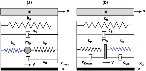
Given these comparative advantages, this paper focuses on passive vibration control strategies and, specifically, on the KDamper concept. The KDamper is a recently developed passive DVA that efficiently integrates the advantages of TMDs and NSDs. It offers an optimal combination of positive ($k_P$) and negative ($k_N$) stiffness elements, along with damping elements ($c_D$) and an additional mass ($m_D$) that allows for the transfer of vibrating energy from the structure to the device. Figure 1a schematically illustrates the device working in parallel with a single degree of freedom (SDoF) system of initial stiffness ($k_R$) and damping ($c_s$). The KDamper may be considered an indirect approach to increase the inertia effect of the TMD mass with the NSD force without increasing the additional mass itself. Antoniadis et al. (2016) presented a conceptual study on the fundamentals of the KDamper for improved vibration control. Compared to NSDs, the main advantage of the KDamper is that it requires no reduction in the overall stiffness of the system, thus ensuring static and dynamic stability. Additionally, the device may overcome the sensitivity issues in tuning TMD stiffness and mass since it is mainly controlled by optimally tuning the negative stiffness element.

Figure 1. (a) Original KDamper concept, and (b) Extended KDamper concept.

Kapasakalis et al. (2017) implemented the KDamper to control the vibrations of a wind turbine tower, while Sapountzakis et al. (2017) presented a design methodology for the seismic isolation of bridges employing the same concept. Antoniadis et al. (2019) investigated the effectiveness of the KDamper, considering it as a seismic absorption base for multi-storey buildings, while Sapountzakis et al. (2019) realized the KDamper concept using Belleville (disc) springs. A framework for the optimal design and selection of the KDamper parameters for a typical bridge structure was recently presented based on: (i) response transfer functions; or (ii) an optimization algorithm (Bollano et al. 2021).

The present study investigates an Extension of the KDamper (EKD) concept. As shown in Fig. 1b, the EKD differs from the KDamper in the arrangement of its stiffness elements and the number of employed viscous dampers. Compared to the original KDamper, the technical implementation of the EKD is more straightforward for two main reasons: (i) The negative stiffness element is no longer subject to gravitational forces, as it is not responsible for supporting the additional mass, $m_D$. This factor had previously complicated its realistic design (e.g., via precompressed springs) due to the weight of the additional mass; (ii) The additional mass is now supported by the positive stiffness element, which can provide the necessary vertical rigidity, when realized, for instance, through conventional elastomeric bearings. Recently, the EKD has been implemented for the passive vibration control of offshore wind turbines (Kampitsis et al. 2022) and the seismic protection of reinforced concrete (RC) buildings (Kapasakalis et al. 2021; Mantakas et al. 2022).

The EKD is expected to outperform the KDamper due to the integration of viscous dampers ($C_{\mathit{up}}$, $C_{\mathit{down}}$) working in parallel with each stiffness element. The dampers enhance the absorber’s dynamic behaviour by effectively reducing the system’s seismic displacements. At the same time, they also reduce the negative stiffness element stroke, i.e. the maximum relative displacement between its two endpoints, thereby eliminating any construction limitations that may arise from significantly large stroke values. A direct comparison of the two devices, as presented in Kapasakalis et al. (2021) using a three-story building as the test case, reveals that the EKD consistently outperforms the KDamper when both are designed following the same optimization procedure. Notably, the EKD reduces the relative structural displacement and the stroke of the negative stiffness element by at least 50% in all examined cases.

In the following sections, the EKD is implemented as the seismic protection system of a benchmark highway bridge. While the concept is not being introduced for the first time herein, this work incorporates several novel features that improve understanding of the EKD dynamic behaviour and assist in recognizing both the advantages and limitations of its application as a seismic protection measure for bridge structures. The key features and novelties of the current research can be summarized as follows:

1. A design framework for the EKD devices is introduced based on current seismic design provisions and a constrained optimization process, where construction limitations for the device components are accounted for. For the first time, the variability of seismic motion is accounted for in the design process. This is achieved by comparing outcomes from the traditional spectral matching approach (where a set of input accelerograms are adjusted so that their response spectrum matches the target design spectrum) to those of a linear scaling approach that retains the original frequency content of the records.

2. For the first time, a more realistic representation of the bridge on EKDs is employed. Past research on the application of the KDamper or EKD concept to bridge structures (Bollano et al. 2021; Sapountzakis et al. 2017) has tackled the issue exclusively in linear terms. To address this gap, rigorous Finite Element (FE) analysis using nonlinear constitutive models is conducted to examine the effects of structural and EKD nonlinearities and soil-structure interaction on the overall system dynamics. Capturing the nonlinear response refines the dynamic analysis, facilitating the examination of bridge performance under high-intensity shaking, where the pier may exhibit nonlinear behaviour, EKD nonlinearities may induce residual deck drifts, and the deck may pound on the abutments, potentially altering the intended EKD response.

3. The EKD performance is compared to conventional base isolation (BI) for the benchmark bridge. The results indicate a superior performance for the EKD device, particularly with respect to seismic displacement reduction, hence highlighting its potential as a promising seismic protection technology for bridges.

2. Implementation of the EKD to the Seismic Isolation of RC Bridges

A benchmark highway bridge, initially designed with a conventional seismic isolation (CSI) system, is employed for the case study presented herein (Fig. 2). The bridge has been previously used in the work of Sapountzakis et al. (2017) and Bollano et al. (2021) as a test case for passive control systems based on the KDamper concept.

Figure 2. Geometric configuration of the benchmark highway bridge supported on conventional elastomeric bearings.

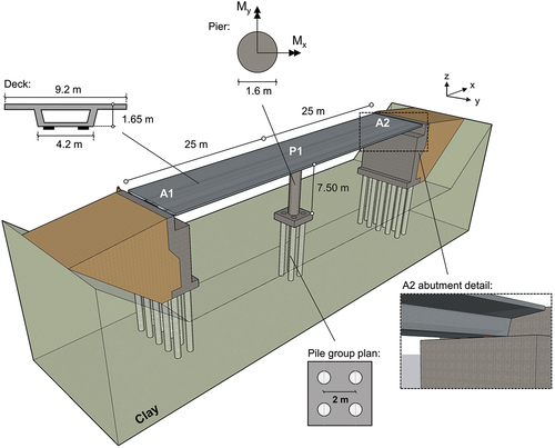
It consists of an essentially rigid continuous deck of mass $m_s$ = 729.3 Mg, with two 25 m long spans supported on elastomeric bearings, sitting on seat-type abutments and a single RC pier (C30/37). Five conventional ALGABLOC NB 400 × 500/99/71 bearings are used, two above each of the abutments and one above the pier, with horizontal stiffness $k_b$ = 2730 kN/m. The bridge deck is 9.2 m wide, while the pier is cylindrical, with diameter $\mathit{D}$ = 1.6 m and height $\mathit{H}$ = 7.5 m. Based on its geometrical characteristics, the pier stiffness is $k_{\mathit{pier}}$ = 73344 kN/m (assuming cantilever response and uncracked RC section). This yields a fundamental natural period equal to $T_n=2\mathit{\pi }\sqrt{\frac{{\mathit{m}}_{\mathit{deck}}}{K_{\mathit{tot}}}}$ = 1.45 s, where $K_{\mathit{tot}}=4k_b+\frac{{\mathit{k}}_{\mathit{pier}}{k}_b}{k_{\mathit{pier}}+k_b}$. The pier is founded on stiff clay of undrained shear strength $S_u$ = 150 kPa and $E_o/S_u$ = 1000 (where $E_o$ is the small-strain elastic soil modulus) on a 2 × 2 pile group. The piles feature a diameter $\mathit{D}$ = 0.8 m, spacing $\mathit{s}$ = 2 m, and length-to-diameter ratio $\mathit{L}/\mathit{d}$ = 12. Due to the seismic isolation, no significant discrepancies are expected between the bridge response in the longitudinal (x-axis) and transverse (y-axis) directions. The former is selected for the numerical study.

2.1. Bridge with EKD Devices: System Configuration and Preliminary Design

A potential schematic configuration of the EKD on a bridge structure is illustrated in Fig. 3. The additional mass $m_D$ is materialized by a stack of steel plates (No.1) sitting on conventional isolation bearings (No.2), which play the role of the positive stiffness element $k_P$ (Fig. 3a). The negative stiffness $k_N$ is achieved through a highly compressed machined spring with a double chevron, self-containing frame (No.3), modelled after the design of the negative stiffness device proposed by Sarlis et al. (2013) (Fig. 3b). The precompressed spring is connected to the upper and lower parts of the frame with pinned connections that transfer horizontal loads. When the device deforms in one direction, the precompressed spring rotates, and its force assists the motion rather than resisting it (creation of negative stiffness).

Figure 3. Schematic implementation of the EKD on a bridge: (a) transverse cross-section of the bridge, with the EKD device located at the deck – pier interface (the viscous dampers are not shown for clarity); (b) plan view of the negative stiffness elements, following the design proposed by Sarlis et al. (2013); and (c) longitudinal cross-section of the bridge, highlighting the position of the viscous dampers.

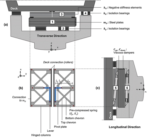
Implementation of the negative stiffness element (NSE) is assumed to follow the horizontal NSD arrangement of Attary et al. (2015b), who used such devices for the seismic control of a bridge tested on a shaking table. Two NSE assemblies are required per EKD to exert symmetric shear forces to the deck during shaking and eliminate the possibility of torsion (Fig. 3b). On the one side, the self-containing frames are rigidly connected at the top of the additional mass $m_D$. On the other side, the NSEs are attached to the underside of the deck. Since the width of the self-containing frame decreases during seismic loading, the side of the NSE that is attached to the deck is thought to be located within an adjustable cap that contains roller plates to allow shearing deformation of the frame (change of width) and simultaneous transfer of NSE forces to the deck (Attary et al. 2015b). The EKD is complemented by viscous dampers ($C_{\mathit{up}},C_{\mathit{down}}$) that work in parallel with the positive and negative stiffness elements to control displacements (No.5 and No.6 in Fig. 3c), while the entire device works in parallel with conventional isolation bearings (No. 4 in Fig. 3a) that represent the stiffness $k_R$. In this preliminary configuration, the NSEs are arranged to apply force along the longitudinal bridge direction, and thus, additional NSEs would be required to apply negative stiffness force in the transverse direction. More specifically, the layout of the negative stiffness elements would necessitate expansion to include four elements per EKD device, positioned radially; that is, two precompressed springs would need to be operative in each lateral direction. Similarly, additional viscous dampers, functioning alongside the positive and negative stiffness elements, would be required in the transverse direction. In this context, the EKD design procedure would have to meticulously consider the increased horizontal space requirements of a bi-directional EKD. Alternatively, subject to the available height between the pier and the deck, the design of the negative stiffness element and its accompanying viscous dampers ($C_{\mathit{up}}$) could be modified to align with the arrangement presented in Kampitsis et al. (2022), where the precompressed springs are placed vertically, thus working interchangeably in both directions.

2.2. Simplified Analytical Model

A linear two-degree of freedom (2-DoF) mathematical model is selected to represent the dynamics of the original bridge on CSI under seismic shaking in the longitudinal direction, where the deck, the bearings and the flexible pier are simulated with concentrated masses, associated stiffness and damping elements. Considering a rigid deck response, such simplification is not expected to significantly affect the seismic performance of the system when subjected to one-dimensional shaking (Bhuiyan and Alam 2013; Kunde and Jangid 2006). Soil-structure interaction (SSI) is ignored at this stage, assuming rigid base conditions. The equations of motion for the 2-DoF system subjected to ground acceleration ${\ddot{x}}_{\mathit{G}}\left(\mathit{t}\right)$ are provided in Appendix A.

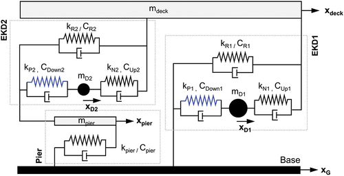
Seismic isolation of the bridge with EKDs assumes placement of the devices at the deck-support (pier or abutment) interface. Different properties are considered for the EKDs placed at the abutments and the pier, marked henceforth with indices $\mathit{i}$ = 1 and 2, respectively. The EKDs addition increases the system’s DoFs, resulting in the linear 4-DoF mathematical model displayed in Fig. 4, which is subsequently used to optimize the EKD design parameters. It is acknowledged that the employed 1-dimensional model cannot capture the torsional motion potentially arising from disparities in the properties of the different EKD devices (Matsagar and Jangid 2006). An additional rotational degree-of-freedom for the deck would be necessary to fully account for this feature. Nevertheless, to maintain simplicity, the effect of torsion is not examined herein; future research efforts will thoroughly investigate the impact of such simplification on the system’s dynamic performance.

Figure 4. Simplified mathematical model representing the examined bridge equipped with EKD devices.

The equations of motion of the 4-DoF system subjected to ground acceleration ${\ddot{x}}_{\mathit{G}}\left(\mathit{t}\right)$ may be expressed in a matrix form, involving matrices with dimensions $\mathit{r}\times \mathit{r}$ (where $\mathit{r}$ = $\mathit{n}$ +2, and $\mathit{n}=2$ are the DoFs of the bridge on conventional isolation bearings):

(1) $\left[\mathit{M}\right]\left[\ddot{u}\left(\mathit{t}\right)\right]+\left[\mathit{C}\right]\left[\dot{u}\left(\mathit{t}\right)\right]+\left[\mathit{K}\right]\left[\mathit{u}\left(\mathit{t}\right)\right]=-\left[\mathit{M}\right]{\mathbf{1}}_r^T{\ddot{x}}_{\mathit{G}}(\mathit{t})$(1)

where the matrices and vectors entering Eq. (1)(1) $\left[\mathit{M}\right]\left[\ddot{u}\left(\mathit{t}\right)\right]+\left[\mathit{C}\right]\left[\dot{u}\left(\mathit{t}\right)\right]+\left[\mathit{K}\right]\left[\mathit{u}\left(\mathit{t}\right)\right]=-\left[\mathit{M}\right]{\mathbf{1}}_r^T{\ddot{x}}_{\mathit{G}}(\mathit{t})$(1) are defined as

(2a) ${\left[M\right]}_{\mathit{r}\times \mathit{r}}=\left[\begin{array}{ccc}{\left[{\mathit{M}}_{\mathit{CSI}}\right]}_{\mathit{n}\times \mathit{n}}& {\left[0\right]}_{\mathit{n}\times 1}& {\left[0\right]}_{\mathit{n}\times 1}\\ {\left[0\right]}_{1\times \mathit{n}}& m_{\mathit{D}1}& 0\\ {\left[0\right]}_{1\times \mathit{n}}& 0& m_{\mathit{D}2}\end{array}\right]$(2a)

(2b) ${\left[K\right]}_{\mathit{r}\times \mathit{r}}=\left[\begin{array}{cc}{\left[{\mathit{K}}_{\mathit{CSI}}\right]}_{\mathit{n}\times \mathit{n}}& {\left[0\right]}_{\mathit{n}\times \mathit{n}}\\ {\left[0\right]}_{\mathit{n}\times \mathit{n}}& {\left[0\right]}_{\mathit{n}\times \mathit{n}}\end{array}\right]\mathit{\hspace{0.17em}}+\left[\begin{array}{cccc}{k}_{\mathit{P}2}& 0& 0& -k_{\mathit{P}2}\\ 0& k_{\mathit{N}1}+k_{\mathit{N}2}& -k_{\mathit{N}1}& -k_{\mathit{N}2}\\ 0& -k_{\mathit{N}1}& k_{\mathit{N}1}+k_{\mathit{P}1}& 0\\ -k_{\mathit{P}2}& -k_{\mathit{N}2}& 0& k_{\mathit{N}2}+k_{\mathit{P}2}\end{array}\right]$(2b)

(2c) ${\left[C\right]}_{\mathit{r}\times \mathit{r}}=\left[\begin{array}{cc}{\left[{\mathit{C}}_{\mathit{CSI}}\right]}_{\mathit{n}\times \mathit{n}}& {\left[0\right]}_{\mathit{n}\times \mathit{n}}\\ {\left[0\right]}_{\mathit{n}\times \mathit{n}}& {\left[0\right]}_{\mathit{n}\times \mathit{n}}\end{array}\right]+\left[\begin{array}{cccc}{C}_{\mathit{Down}2}& 0& 0& -C_{\mathit{Down}2}\\ 0& C_{\mathit{Up}1}+C_{\mathit{Up}2}& -C_{\mathit{Up}1}& -C_{\mathit{Up}2}\\ 0& -C_{\mathit{Up}1}& C_{\mathit{Up}1}+C_{\mathit{Down}1}& 0\\ -C_{\mathit{Down}2}& -C_{\mathit{Up}2}& 0& C_{\mathit{Up}2}+C_{\mathit{Down}2}\end{array}\right]$(2c)

(2d) ${\left[\mathit{u}\left(\mathit{t}\right)\right]}_{\mathit{r}\times 1}=\left[\begin{array}{c}{\left[\mathit{u}{\left(\mathit{t}\right)}_{\mathit{CSI}}\right]}_{\mathit{n}\times 1}\\ u_{\mathit{D}1}\left(\mathit{t}\right)\\ u_{\mathit{D}2}\left(\mathit{t}\right)\end{array}\right]$(2d)

In Eq. (2):(2a) ${\left[M\right]}_{\mathit{r}\times \mathit{r}}=\left[\begin{array}{ccc}{\left[{\mathit{M}}_{\mathit{CSI}}\right]}_{\mathit{n}\times \mathit{n}}& {\left[0\right]}_{\mathit{n}\times 1}& {\left[0\right]}_{\mathit{n}\times 1}\\ {\left[0\right]}_{1\times \mathit{n}}& m_{\mathit{D}1}& 0\\ {\left[0\right]}_{1\times \mathit{n}}& 0& m_{\mathit{D}2}\end{array}\right]$(2a)

• ${\left[{\mathit{M}}_{\mathit{CSI}}\right]}_{\mathit{n}\times \mathit{n}}$, ${\left[{\mathit{K}}_{\mathit{CSI}}\right]}_{\mathit{n}\times \mathit{n}}$ and ${\left[{\mathit{C}}_{\mathit{CSI}}\right]}_{\mathit{n}\times \mathit{n}}$ are 2-dimensional matrices of mass, stiffness, and damping of the bridge on isolation bearings, equivalent to the ones provided in Appendix A for the linear 2-DoF system. The isolation bearings represent elements $k_{\mathit{R}1},C_{\mathit{R}1}$ and $k_{\mathit{R}2},C_{\mathit{R}2}$ in Fig. 4, i.e. the stiffness and damping of the elements working in parallel with the EKDs devices. With reference to Appendix A, coefficients $k_{\mathit{R}1},C_{\mathit{R}1}$ and $k_{\mathit{R}2},C_{\mathit{R}2}$ are the equivalent of $k_{\mathit{b}1},c_{\mathit{b}1}$ and $k_{\mathit{b}2}$, $c_{\mathit{b}2}$ in the original bridge configuration.

• The vector ${\left[\mathit{u}{\left(\mathit{t}\right)}_{\mathit{CSI}}\right]}_{\mathit{n}\times 1}$ = ${\left[{\mathit{u}}_{\mathit{pier}}\left(\mathit{t}\right),u_{\mathit{deck}}\left(\mathit{t}\right)\right]}^{\mathit{T}}$ represents the relative to the ground displacements of the pier and deck masses, where $u_{\mathit{pier}}\left(\mathit{t}\right)$ = $x_{\mathit{pier}}\left(\mathit{t}\right)$ - $x_G\left(\mathit{t}\right)$ and $u_{\mathit{deck}}\left(\mathit{t}\right)$ = $x_{\mathit{deck}}\left(\mathit{t}\right)$ - $x_G\left(\mathit{t}\right)$.

• $u_{\mathit{D}1}\left(\mathit{t}\right)$ = $x_{\mathit{D}1}\left(\mathit{t}\right)$ - $x_G\left(\mathit{t}\right)$ and $u_{\mathit{D}2}\left(\mathit{t}\right)$ = $x_{\mathit{D}2}\left(\mathit{t}\right)$ - $x_G\left(\mathit{t}\right)$ are the drifts of the internal DoFs representing the masses of the EKD devices at the abutments and the pier, respectively.

• ${{\mathbf{1}}_{\mathbf{r}}}^{\mathit{T}}$ is an $\mathit{r}$x$1$ vector of ones (influence vector in the case of horizontal, one-dimensional ground shaking).

With the aid of algebraic manipulations, Eq. (1)(1) $\left[\mathit{M}\right]\left[\ddot{u}\left(\mathit{t}\right)\right]+\left[\mathit{C}\right]\left[\dot{u}\left(\mathit{t}\right)\right]+\left[\mathit{K}\right]\left[\mathit{u}\left(\mathit{t}\right)\right]=-\left[\mathit{M}\right]{\mathbf{1}}_r^T{\ddot{x}}_{\mathit{G}}(\mathit{t})$(1) may be further transformed into the following set of equations:

(3a) $m_{\mathit{pier}}{\ddot{u}}_{\mathit{pier}}+(C_{\mathit{pier}}+C_{\mathit{R}2}+C_{\mathit{Down}2}){\dot{u}}_{\mathit{pier}}-C_{\mathit{Down}2}{\dot{u}}_{\mathit{D}2}-C_{\mathit{R}2}{\dot{u}}_{\mathit{deck}}+\left(k_{\mathit{pier}}+k_{\mathit{R}2}+k_{\mathit{P}2}\right)u_{\mathit{pier}}-k_{\mathit{P}2}{u}_{\mathit{D}2}-k_{\mathit{R}2}{u}_{\mathit{deck}}=-m_{\mathit{pier}}{\ddot{x}}_{\mathit{G}}$(3a)

(3b) $m_{\mathit{D}1}{\ddot{u}}_{\mathit{D}1}+(C_{\mathit{Up}1}+C_{\mathit{Down}1}){\dot{u}}_{\mathit{D}1}-C_{\mathit{Up}1}{\dot{u}}_{\mathit{deck}}+\left(k_{\mathit{P}1}+k_{\mathit{N}1}\right)u_{\mathit{D}1}-k_{\mathit{N}1}{u}_{\mathit{deck}}=-m_{\mathit{D}1}{\ddot{x}}_{\mathit{G}}$(3b)

(3c) $m_{\mathit{D}2}{\ddot{u}}_{\mathit{D}2}-C_{\mathit{Down}2}{\dot{u}}_{\mathit{pier}}+(C_{\mathit{Up}2}+C_{\mathit{Down}2}){\dot{u}}_{\mathit{D}2}-C_{\mathit{Up}2}{\dot{u}}_{\mathit{deck}}-k_{\mathit{P}2}{u}_{\mathit{pier}}+(k_{\mathit{P}2}+k_{\mathit{N}2})u_{\mathit{D}2}-k_{\mathit{N}2}{u}_{\mathit{deck}}=-m_{\mathit{D}2}{\ddot{x}}_{\mathit{G}}$(3c)

(3d) $m_{\mathit{deck}}{\ddot{u}}_{\mathit{deck}}-C_{\mathit{R}2}{\dot{u}}_{\mathit{pier}}-C_{\mathit{Up}1}{\dot{u}}_{\mathit{D}1}-C_{\mathit{Up}2}{\dot{u}}_{\mathit{D}2}+(C_{\mathit{R}1}+C_{\mathit{R}2}+C_{\mathit{Up}1}+C_{\mathit{Up}2}){\dot{u}}_{\mathit{deck}}-k_{\mathit{R}2}{u}_{\mathit{pier}}-k_{\mathit{N}1}{u}_{\mathit{D}1}-k_{\mathit{N}2}{u}_{\mathit{D}2}+\left(k_{\mathit{R}1}+k_{\mathit{R}2}+k_{\mathit{N}1}+k_{\mathit{N}2}\right)u_{\mathit{deck}}=-m_{\mathit{deck}}{\ddot{x}}_{\mathit{G}}$(3d)

In reality, structural parameters (mass, stiffness, and damping) and boundary conditions are not known precisely, leading to a significant amount of uncertainty in modelling the response of dynamic systems. The employed 4-DoF mathematical model accounts for two such types of uncertainty:

1. Uncertainty in the mechanical parts of the EKDs (e.g. Papadimitriou et al. 1997), which is represented in the model by the terms ${\epsilon }_N$, ${\epsilon }_P$ and ${\epsilon }_R$ that correspond to variations in the negative and positive stiffness elements (refer to Section 3 for further details). Such variations may occur due to several reasons, such as temperature changes, manufacturing tolerances, and nonlinear behaviour of the structural elements.

2. Uncertainty in the seismic excitation parameters: the dynamic performance of the examined structural system strongly depends on the excitation characteristics, such as frequency content, maximum acceleration, and significant duration. Aiming to incorporate the effect of seismic motion variability in the design process of the EKDs, an ensemble of 20 real accelerograms from international ground motion databases (e.g. the PEER Strong Ground Motion Database¹) is used, along with two different spectral matching techniques (refer to Section 3 for further details).

3. EKD design optimization

The device design is optimized through a constrained optimization process, aiming to obtain a set of optimal EKD parameters that will minimize the relative displacement of the isolated deck while ensuring that its acceleration will not exceed a predefined threshold. For this purpose, the Harmony Search (HS) algorithm – a novel metaheuristic algorithm – is employed. Due to its simple algorithmic nature and efficient search capacity, the HS algorithm has been successfully employed in previous studies for the optimal design of passive vibration absorbers (e.g. Kapasakalis et al. 2021; Nigdeli and Bekdaş 2017). The algorithm stands out for its ability to handle problems that incorporate discrete and continuous variables. Moreover, it employs a stochastic random search, a notable divergence from the gradient search approach typically seen in conventional optimization approaches. This method equips the algorithm with a broader exploration scope across the search space, thereby reducing the risk of entrapment in local optima. The basic calculation steps involved in the HS algorithm are briefly described in Appendix B.

3.1. Fixed Parameters

The following parameters are considered fixed with regard to the optimization problem:

1. The pier stiffness, $k_{\mathit{pier}}$ = 73344 kN/m. Given the non-monolithic nature of the bridge-deck connection due to seismic isolation, the target is to achieve an elastic pier response, and hence, the analysis assumes uncracked RC section behaviour. However, it is advisable to solve the problem using both the cracked and uncracked RC pier stiffness properties and evaluate the results comparatively to decide upon the final design solution. In our case, assuming cracked pier stiffness properties ($k_{\mathit{pier},\mathit{cracked}}$ = 45211 kN/m in accordance with EC8 2005) led to only limited variations in the derived EKD design variables.

2. The pier and deck mass: $m_{\mathit{pier}}$ = 36.2 Mg, $m_{\mathit{deck}}$ = 729.3 Mg.

3. The EKDs masses: $m_{\mathit{D}1}$ = 4% $m_{\mathit{Deck}}$, $m_{\mathit{D}2}$ = 1% $m_{\mathit{Deck}}$. The EKD masses account for 5% of the total deck mass, following previous work on the KDamper (e.g. Antoniadis et al. 2019; Kapasakalis et al. 2019), thus yielding an efficient and realistic configuration.

4. The variation of positive and negative stiffness elements (${\epsilon }_N$, ${\epsilon }_P,{\epsilon }_R$), which is set to 10%, following the study of Kapasakalis et al. (2021). This results in a relatively conservative EKD design, in contrast with previous studies on the KDamper (e.g. Antoniadis et al. 2019; Kapasakalis et al. 2019), where factor ${\epsilon }_N$ was assumed to be 5%.

3.2. Dependent and Independent Design Variables

Eight independent design variables are optimized under the proposed method:

• $k_{\mathit{N}1},k_{\mathit{N}2}$ : stiffness of the negative stiffness elements

• $C_{\mathit{Down}1}$, $C_{\mathit{Down}2}$, $C_{\mathit{Up}1}$, $C_{\mathit{Up}2}$ : damping coefficients of the EKD viscous dampers

• $k_{\mathit{R}1}$ , $k_{\mathit{R}2}$ : horizontal stiffness of the isolation bearings working in parallel with the EKDs

The total stiffness $k_o$ of each EKD assembly can be expressed using the following formula:

(4) $k_o=k_R+\frac{k_P{k}_N}{k_{\mathit{P}}+k_N}$(4)

Assuming variation in the positive and negative stiffness elements, and more specifically, an increase in the absolute value of $k_N$ by a factor ${\epsilon }_N$, and/or a decrease in the absolute values of $k_P$ or $k_R$ by ${\epsilon }_P$ and ${\epsilon }_R$, the total stiffness of the assembly can theoretically be zeroed, yielding the following marginal horizontal stability criterion:

(5) $k_o=0\leftrightarrow \left(1-{\epsilon }_R\right)k_R+\frac{\left(1-{\epsilon }_P\right)k_P\left(1+{\epsilon }_N\right)k_N}{\left(1-{\epsilon }_P\right)k_{\mathit{P}}+\left(1+{\epsilon }_N\right)k_N}=0$(5)

To ensure that potential loss of the EKD static stability is prevented, the positive stiffness elements $k_{\mathit{P}1}$ and $k_{\mathit{P}2}$ are derived as dependent variables from Eq. (5)(5) $k_o=0\leftrightarrow \left(1-{\epsilon }_R\right)k_R+\frac{\left(1-{\epsilon }_P\right)k_P\left(1+{\epsilon }_N\right)k_N}{\left(1-{\epsilon }_P\right)k_{\mathit{P}}+\left(1+{\epsilon }_N\right)k_N}=0$(5) for each solution vector of independent design variables.

Moreover, the damping matrix ${\left[{\mathit{C}}_{\mathit{CSI}}\right]}_{\mathit{n}\times \mathit{n}}$, which is not explicitly known upon analysis initiation, is calculated under the assumption of mass and stiffness proportional damping using the same damping ratio in all eigenmodes ($\mathit{\xi }$ = 5%, considered representative of both the reinforced concrete pier and the elastomeric bearings selected to work in parallel with the EKD devices).

3.3. Selection of Earthquake Ground Motions

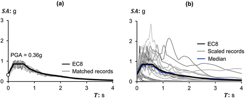
The optimization problem is formed according to current seismic design codes. The EC8 design response spectrum is employed to specify seismic demand. A database of 20 real accelerograms (Table 1) recorded on Soil Type B or C is manipulated to match the target EC8 spectrum for Type C soil, $\mathit{PGA}$ = 0.36 g, spectrum type I, and importance class II. Two different strategies are followed to produce spectrum-compatible acceleration time series:

• Method A (one-by-one spectral match): The records are manipulated in the frequency domain to match the target spectrum, employing SeismoMatch (Seismosoft 2020). Several physical characteristics of the seismic motion (e.g. number of cycles) are retained, making the technique more appealing compared to the generation of spectrum-compatible artificial motions.

• Method B (Median spectral match): The records are scaled linearly (uniform amplification or contraction) without changing their frequency content, with scale factors limited in the range of 0.5 < Scale Factor < 2.4. The procedure is iterative, with the scale factors being readjusted until obtaining the best fit of the average produced spectrum to the target EC8 spectrum. The Peak Ground Acceleration ($\mathit{PGA}$), maximum spectral acceleration and scale factors of the modified Method B records are tabulated in Table 1.

Table 1. Real records manipulated to match the target EC8 spectrum.

Record No.	Name	Method B scale factor	PGA*: g	SAmax*: g	T [SAmax] *: s
1	Lytle Creek, US, 1970 (Wrightwood − 6074 Park)	0.7	0.10	0.26	0.05
2	Erzincan, Turkey, 1992	0.6	0.29	0.89	0.06
3	Northern Calif-03, US, 1954 (Ferndale City Hall)	0.7	0.11	0.33	0.08
4	Superstition Hills-02, US, 1987 (El Centro Imp. Co cent.)	0.8	0.27	0.68	0.04
5	Whittier Narrows-01, US, 1987 (Brea Dam)	0.7	0.12	0.47	0.04
6	Morgan Hill, US, 1984 (Anderson Dam)	0.6	0.25	0.66	0.09
7	Irpinia, Italy, 1980 (Brienza)	2.0	0.35	1.37	0.14
8	Laquila, Italy, 2009 (ACV)	1.0	0.66	1.76	0.11
9	Friuli 3rd Shock, Italy, 1976 (E.FRC)	1.7	0.57	1.97	0.49
10	Emilia-Romagna, Italy, 2012 (Mirandola)	1.2	0.31	1.30	0.27
11	Tabas, Iran, 1978	0.5	0.42	1.68	0.24
12	El Salvador, US, 1986 (NGI_180)	1.5	0.59	1.31	0.84
13	San Fernando, California, US, 1971 (Pacoima dam_254)	0.6	0.69	1.56	0.42
14	Northridge, US, 1994 (Jensen292)	1.6	0.68	1.82	0.77
15	Loma Prieta, US, 1989 (Gilroy #2)	1.2	0.43	1.71	0.39
16	Loma Prieta, US, 1989 (Treasure Island 090)	2.1	0.34	1.56	0.65
17	Lefkada, Greece, 2003	2.0	0.70	2.86	0.53
18	Kocaeli, Turkey, 1999 (Yarimca)	2.0	0.54	1.56	0.53
19	Kobe, Japan, 1995 (Takatori 000)	1.0	0.61	2.15	1.23
20	Imperial Valley, El Centro, US, 1940 (El Centro_270)	2.4	0.52	1.42	0.29

*The values correspond to spectral matching with Method B.

Figure 5 compares the EC8 design response spectrum with the acceleration response spectra of the 20 manipulated records for Methods A and B. Although Method A is widely used in practice, the generated motions are often criticized for being unrealistic. The EC8 design spectrum represents an envelope of possible spectral accelerations rather than a single event, leading to motions with distorted frequency content when Method A is employed. In contrast, Method B preserves the original motions’ frequency content and physical characteristics, making it a more realistic approach when the employed scaling factors are limited within suitable boundaries.

Figure 5. Elastic response spectra of the modified records matched to the EC8 design response spectrum using: (a) Method A; and (b) Method B.

3.4. Optimization Objective Function and Constraints

For the optimal design of EKD parameters, the 4-DoF linear mathematical model is analyzed in the time domain, using the 20 accelerograms of the previous section as excitation. The Newmark method is employed to solve the system of differential equations. It is noted that:

1. The deck drift is set as the objective function. The algorithm calculates the mean value of absolute maximum deck drift [$\mathit{mean}\left(\mathit{max}\left|{\delta }_{\mathit{Deck}}\right|\right)$] stemming from the model’s time-domain analyses using the 20 spectrum-compatible motions.

2. An acceleration filter ($\mathit{AF}$) is placed to the deck acceleration, expressed as a percentage of the mean applied $\mathit{PGA}$. More specifically, the average value of the absolute maximum deck acceleration $\mathit{mean}\left(\mathit{max}\left|a_{\mathit{Deck}}\right|\right)$ ≤70% $\times$ $\mathit{mean}\left(\mathit{PGA}\right)$.

Based on feasibility and technical limitations, appropriate limits are set to the independent design variables to achieve values within a reasonable/technologically applicable range (Table 2). The limits are applied considering the placement of eight EKD devices at the abutments (four on each side) and one at the pier. More specifically:

• An upper limit of $\left|k_N\right|$ = 2000 kN/m is set for the NSEs. This is mandated by dimension limitations for the NSE setup (i.e. the requirement to fit the devices in the available space at the deck-pier and deck-abutment interface), and the range of plausible stiffness ($K_s$) and precompression load ($F_p$) of the mechanical springs (Fig. 3b). A maximum $\left|k_N\right|$ = 18000 kN/m is considered for the entire bridge, corresponding to a total deck mass of 729 Mg. This is significantly lower than what has been proposed in previous indicative designs of the KDamper concept, realized with precompressed springs (e.g. Antoniadis et al., 2018), yet closer to the value proposed by Kapasakalis et al. (2021), where $\left|k_N\right|$ <17500 kN/m was assumed for a total superstructure mass of 300 Mg.

• The maximum value of the damping coefficients is set to 100 kNs/m per damper, allowing the use of common seismic dampers for the specific space requirements (Enidine 2022).

• The stiffness of positive stiffness elements $k_R$ ranges between 1000 and 3200 kN/m, assuming that standard elastomeric bearings that respect the space limitations will be used. The $k_R$ value represents the horizontal stiffness of the isolation bearings, calculated as $K_{\mathit{b},\mathit{H}}=\mathit{GA}/\sum t_r$ (Kelly 1997), where $\mathit{G}$ = 0.9 MPa is the shear modulus of rubber, $\mathit{A}$ is the bearing area, and $\sum t_r$ is the total height of the elastomer, set as 0.15 m. A similar constraint is set for the calculated stiffness of $k_P$ elements.

Table 2. Limits set to the free design variables of the optimization problem.

	$\mathit{EK}{\mathit{D}}_{\left(\mathit{i}=1\right)}\mathit{\hspace{0.17em}}$: Abutments (values per EKD)				$\mathit{EK}{\mathit{D}}_{\left(\mathit{i}=2\right)}\mathit{\hspace{0.17em}}$: Pier
Parameter	$k_{\mathit{N}1}$ (kN/m)	$k_{\mathit{R}1}$ (kN/m)	$C_{\mathit{Up}1}$ (kNs/m)	$C_{\mathit{Down}1}$ (kNs/m)	$k_{\mathit{N}2}$ (kN/m)	$k_{\mathit{R}2}$ (kN/m)	$C_{\mathit{Up}2}$ (kNs/m)	$C_{\mathit{Down}2}$ (kNs/m)
Value range	[−1–2000]	[1000 3200]	[1 100]	[1 100]	[−1–2000]	[1000 3200]	[1 100]	[1 100]

3.5. Optimization Results

The sets of optimized EKD parameters obtained with Methods A and B are summarized in Table 3. The dynamic response of the system (in terms of mean absolute maximum deck drift) is also included in the table: $\mathit{mean}\left[\mathit{max}\left|{\delta }_{\mathit{Deck}}\right|\right]$. It is noted that the $\mathrm{EK}{\mathrm{D}}_{\left(\mathit{i}\mathit{\hspace{0.17em}}=\mathit{\hspace{0.17em}}1\right)}$ parameters refer to individual devices (i.e. four devices above each abutment). Both solutions (Methods A and B) result in approximately the same dynamic response in terms of mean deck drift (0.075 for Method A vs. 0.081 for Method B), mobilizing, however, different values of the independent design variables. Method B requires 3.5 times larger negative stiffness at the pier [$\mathrm{EK}{\mathrm{D}}_{\left(\mathit{i}\mathit{\hspace{0.17em}}=\mathit{\hspace{0.17em}}2\right)}$], larger $k_R$ elements, and significantly larger viscous damping coefficients (for both $\mathrm{EK}{\mathrm{D}}_{\left(\mathit{i}\mathit{\hspace{0.17em}}=\mathit{\hspace{0.17em}}1\right)}$ and $\mathrm{EK}{\mathrm{D}}_{\left(\mathit{i}\mathit{\hspace{0.17em}}=\mathit{\hspace{0.17em}}2\right)}$) compared to Method A, in order to achieve similar performance in terms of $\mathit{mean}\left[\mathit{max}\left|{\delta }_{\mathit{Deck}}\right|\right]$. We eventually adopt the EKD design that is derived using Method B, as it is considered more realistic and clearly more conservative. The aim is to increase the efficiency of the EKD for a range of seismic scenarios with different excitation characteristics. For the selected set of optimized parameters, the positive stiffness element values $k_{\mathit{P}1}$ and $k_{\mathit{P}2}$ are calculated as 2058.5 kN/m and 1046.3 kN/m, respectively (Eq. 5(5) $k_o=0\leftrightarrow \left(1-{\epsilon }_R\right)k_R+\frac{\left(1-{\epsilon }_P\right)k_P\left(1+{\epsilon }_N\right)k_N}{\left(1-{\epsilon }_P\right)k_{\mathit{P}}+\left(1+{\epsilon }_N\right)k_N}=0$(5) ). The addition of EKDs increases the natural period of the system to $T_n$ = 1.75s.

Table 3. Set of optimized parameters for the bridge EKDs.

			$\mathit{EK}{\mathit{D}}_{\left(\mathit{i}=1\right)}\mathit{\hspace{0.17em}}$: Abutments*				$\mathit{EK}{\mathit{D}}_{\left(\mathit{i}=2\right)}\mathit{\hspace{0.17em}}$: Pier
Spectral matching method	$\mathit{mean}$ [$\mathit{max}|{\delta }_{\mathit{Deck}}|]$ (m)	$\mathit{AF}$ (%)	$k_{\mathit{N}1}$ (kN/m)	$k_{\mathit{R}1}$ (kN/m)	$C_{\mathit{Up}1}$ (kNs/m)	$C_{\mathit{Down}1}$ (kNs/m)	$k_{\mathit{N}2}$ (kN/m)	$k_{\mathit{R}2}$ (kN/m)	$C_{\mathit{Up}2}$ (kNs/m)	$C_{\mathit{Down}2}$ (kNs/m)
A	0.075	70	−1072.7	2883.6	99.8	10.8	−174.3	1655.3	15.8	61.8
B	0.081	70	−1011.7	3096.6	90.9	61.6	−604.0	2507.3	98.8	90.5

*The values correspond to individual EKD devices above the abutments.

3.6. Linear Dynamic Performance: EKD Vs Conventional Seismic Isolation (CSI)

The seismic performance of the linear mathematical model equipped with EKDs (Fig. 4) is summarized in Fig. 6 for both Method A and Method B records and compared to the performance of the bridge on conventional seismic isolation (CSI).

Figure 6. Comparative assessment of the initial system on conventional seismic isolation (CSI) and the bridge equipped with EKDs, in terms of maximum deck drift $max|{\delta }_{\mathit{Deck}}|$ and maximum deck acceleration $max\left|{\delta }_{\mathit{Deck}}\right|$ for records obtained using: (a) Method A; and (b) Method B.

As observed, the bridge equipped with EKDs outperforms the initial system (CSI) in terms of maximum deck drift $\mathit{max}\left|{\delta }_{\mathit{Deck}}\right|$ for all examined scenarios, reducing the mean relative displacement by 58% for both Method A (0.075 m vs 0.18 m) and Method B (0.081 m vs 0.19 m) records. At the same time, the proposed concept reduces the maximum deck acceleration compared to CSI, albeit to a lower extent: 36% reduction is measured for Method A, as opposed to 26% for Method B records.

Under Method B records, the highest measured value of deck drift for the bridge with EKDs is $\mathit{max}|{\delta }_{\mathit{Deck}}|$ = 0.26 m. In comparison, the highest deck drift sustained by the CSI system reaches 0.76 m (for the same motion, i.e. record No. 19). In terms of maximum deck acceleration, the bridge with EKDs sustains up to 0.80 g for the high-intensity records of the set, while the CSI system reaches up to 1.46 g.

According to EC8 - Part 2 (2005), the maximum allowed seismic shear strain ${\epsilon }_s$ for bridge isolation bearings (calculated as $d_s$/$\mathit{H}$, where $d_s$ is the bearing drift, and $\mathit{H}$ is the bearing height) should be limited to ${\epsilon }_s$ < 200%. Given the very large deck drifts (Fig. 6), it becomes apparent that the CSI system (comprising elastomeric bearings of dimensions L×W×H = 400 × 500 × 99) marginally conforms to this limitation for Method A records. Most importantly, it significantly exceeds the 200% threshold under the records of Method B, implying that the design is insufficient in this case.

The results indicate that the EKDs work consistently well even when subjected to motions with dominant periods close to the natural period of the EKD-isolated structure ($T_n$ = 1.75 s), in contrast to the CSI system, which is designed to work well only for earthquakes with dominant periods away from the fundamental period of the system ($T_n$ = 1.45 s). As a matter of fact, the systems’ performance is comparable for the modified L’ Aquila ACV record (No. 8 in Fig. 6b), which has a dominant period around $T_E$ = 0.5 s (i.e. away from the natural period of both isolated structures). The EKDs result in slightly lower maximum deck drift (0.065 m vs. 0.1 m) yet higher maximum deck acceleration than the CSI system (0.29 g vs. 0.20 g). However, under the modified Takatori 000 record from Kobe, Japan, 1995 (No. 19 in Fig. 6b), which is strong over the period range 1.1 s − 2.2 s, the EKD system performs substantially better than the CSI system.

For site-specific hazard assessments, where particular motion characteristics are prevalent, the optimization process with Method B could be modified by adding larger weight factors to the transient system response (i.e. the maximum deck drift) under seismic records that exhibit site-specific ground motion characteristics.

4. The Effect of Nonlinearities on System Performance

Sections 4 and 5 investigate the effect of superstructure and substructure nonlinearities on the seismic performance of the EKD using rigorous 3D FE analyses. For this purpose, two types of 3D numerical models are developed in Abaqus (Dassault Systemes 2013). The first focuses on the response of the superstructure (pier – isolation system – deck), while soil – structure interaction (SSI) is merely accounted for in a simplified manner, utilizing elastic springs and dashpots to represent the pile group foundation beneath the pier (Fig. 7). The abutments’ contribution (including the backfill soil and pile groups) is not considered at this stage, thereby narrowing down the variables under consideration, thus facilitating a focused parametric investigation into the impact of EKD nonlinearities on the seismic response of the superstructure. A more detailed FE model is developed later on, including the entire soil – foundation–structure system, and is used to examine the effect of abutment stoppers on the seismic response of the bridge.

Figure 7. Outline of the 3D FE model: (a) superstructure on elastic springs; (b) RC pier modelling details; (c) compressive and tensile concrete stress-strain curves employed for the CDP model.

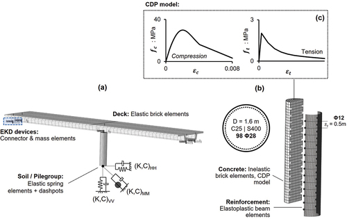
4.1. Numerical Modelling: Superstructure

As already discussed, the pile group is replaced with elastic springs and dashpots in the vertical, horizontal and rotational directions, following the analytical solutions of Dobry and Gazetas (1988) for $\mathit{L}$ = 9.6‬ m long concrete piles of $\mathit{d}$ = 0.8 m diameter, spaced at $\mathit{s}$ = 2 m, with $E_p/E_o$ = 200‬, (here $E_p$ and $E_o$ are the pile and soil stiffness, respectively). The deck is modelled in detail with elastic continuum elements, assuming the properties of reinforced concrete ($\mathit{E}$ = 30 GPa and density $\mathit{\rho }$ = 2.5 Mg/m³). For the simulation of the degrading concrete stiffness and strength, the inelastic RC pier behaviour follows the Concrete Damaged Plasticity (CDP) model (Lee and Fenves 1998). The continuum, plasticity-based damage model captures the effects of irreversible damage associated with concrete’s two main failure mechanisms: tensile cracking and compression crushing. The evolution of the yield surface is controlled by two hardening parameters related to each mechanism, while the development of cracks is macroscopically introduced in the model via a softening stress-strain response. The model follows a yield condition with a non-associated plastic flow rule based on the yield functions proposed by Lubliner et al. (1989) and Lee and Fenves (1998), while the Drucker – Prager hyperbolic function is used as the flow potential. Its capacity to adequately capture the dynamic concrete material response has been repeatedly demonstrated (e.g. Antoniou et al. 2020; Behnam et al. 2018; Sakellariadis et al. 2020; Zoubek et al. 2013).

The basic parameters required for the definition of the CDP model are the concrete dilation angle $\mathit{\psi }$ = 15°, the flow potential eccentricity $\mathit{ϵ}$ = 0.1, the ratio of initial biaxial compressive yield stress to the initial uniaxial compressive yield stress ${\sigma }_{\mathit{bo}}/{\sigma }_{\mathit{co}}$ = 1.16, and the ratio of the second stress invariant on the tensile meridian q(TM) to that of the compressive meridian q(CM) at the initial yield $K_c$ = 2/3. Further details regarding the model can be found in SIMULIA (2014). The characteristic concrete compressive strength f_ck is set to 30 MPa. The tensile strength is calculated according to EC2, as $f_t\mathit{\hspace{0.17em}}\left[\mathrm{MPa}\right]=0.7\mathit{\hspace{0.17em}}\left[0.3\mathit{\hspace{0.17em}}\left(f_c/1000\right){\mathit{\hspace{0.17em}}}^{\frac{2}{3}}\mathit{\hspace{0.17em}}\right]$, while the Young’s modulus is estimated as $\mathit{E}=\mathit{\hspace{0.17em}}8200\mathit{\hspace{0.17em}}\left(f_c/1000\right){\mathit{\hspace{0.17em}}}^{\frac{3}{8}}\mathit{\hspace{0.17em}}=\mathit{\hspace{0.17em}}29360\mathrm{MPa}$, according to Chang and Mander (1994). The Poisson’s ratio is set to $\mathit{\nu }$ = 0.20, while the density equals $\mathit{\rho }$ = 2.4 Mg/m³. The description of the post-yielding concrete behaviour follows Chang and Mander (1994) and Alfarah et al. (2017). The resulting tensile and compressive stress-strain curves are presented in Fig. 7c.

The longitudinal and transverse reinforcement steel bars ($\mathit{S}$400) are explicitly modelled as elastoplastic beam elements (B31) with Young’s Modulus $E_s$ = 210 GPa and yield stress $f_y$ = 400 kPa, embedded in the concrete elements (Fig. 7b). Perfect-bond conditions are assumed between the reinforcement and the concrete. Finally, connector elements (CONN3D) combined with mass elements are used to simulate the positive/negative stiffness and damping of the EKDs at the deck – pier and deck – abutment interface.

4.2. Nonlinearities at the Positive Stiffness Elements ${\mathit{k}}_{\mathit{P}},{\mathit{k}}_{\mathit{R}}$

The simplified 4-DoF model employed for the preliminary EKD design assumes that the response of the positive stiffness elements ($k_P,k_R$) is linear elastic. In reality, however, the shear stress-shear strain response of the elastomeric bearings is hysteretic, with damping ratios typically ranging from 4–10% (Choi 2002). Following relevant studies (Kelly 1997), the lateral behaviour of bearings is approximated in the 3D numerical model using a bilinear law, characterized by three parameters (Fig. 8a): the initial stiffness $k_1$, the post-yield stiffness $k_2$ (= $k_1/$3), and the characteristic strength $\mathit{Q}$, which can be calculated as follows:

Figure 8. (a) Bilinear model employed to model the hysteretic response of the elastomeric bearings ($k_P,k_R$); and (b) nonlinear force – displacement relationship employed for the $k_N$ elements description.

(6) $\mathit{Q}=u_y\left(k_1-k_2\right)$(6)

where $u_y$ is the yield displacement:

(7) $u_y=0.05\sum t_r$(7)

and $t_r$ is the height of each elastomer layer. The effective damping (${\xi }_{\mathit{eff}}$) is calculated from the stress-strain hysteresis loop as follows:

(8) ${\xi }_{\mathit{eff}}=\frac{4\mathit{Q}\left(\mathrm{u}-\mathit{\hspace{0.17em}}{\mathrm{u}}_{\mathrm{y}}\right)}{2\mathit{\pi }{\mathrm{K}}_{\mathrm{eff}}\mathit{\hspace{0.17em}}{\mathrm{u}}^2}$(8)

where $\mathit{u}$ is the bearing deformation and ${\mathrm{K}}_{\mathit{eff}}$ its effective stiffness, defined as the secant slope of the peak-to-peak values in a hysteresis loop:

(9) $K_{\mathit{eff}}=k_2+\mathit{Q}/\mathit{u}$(9)

The vertical bearing stiffness is calculated following Kelly (1997):

(10) $K_{\mathit{b},\mathit{V}}=\frac{{\mathit{E}}_{\mathit{comp}}\mathit{A}}{\sum t_r}$(10)

where $E_{\mathit{comp}}$ is the instantaneous compression modulus of the rubber-steel composite under the specified vertical load, calculated in function of the shape factor $\mathit{S}=\frac{\mathit{LW}}{2\left(\mathit{L}+\mathit{W}\right)t_r}$, the shear modulus of rubber $\mathit{G}$ = 0.9 MPa, and the aspect ratio $\mathit{W}/\mathit{L}$ of the bearing.

The geometric characteristics of the bearings employed for the EKD devices ($k_P,k_R$ elements) are summarized in Table 4. For all bearings, the damping ratio at 100% shear strain is approximately equal to ${\xi }_{\mathit{eff}}$ = 5% of the critical damping from Eq. (8)(8) ${\xi }_{\mathit{eff}}=\frac{4\mathit{Q}\left(\mathrm{u}-\mathit{\hspace{0.17em}}{\mathrm{u}}_{\mathrm{y}}\right)}{2\mathit{\pi }{\mathrm{K}}_{\mathrm{eff}}\mathit{\hspace{0.17em}}{\mathrm{u}}^2}$(8) . The nonlinear bearing behaviour is simulated numerically by assigning an elastoplastic material with user-defined kinematic hardening to the connector elements. It should be noted that the $k_P,k_R$ stiffness values from the preliminary system design are associated here with the post-yielding bearing stiffness $k_2$.

Table 4. Geometry of elastomeric bearings for the EKD devices ($k_R$, $k_P$ elements).

	$\mathit{EK}{\mathit{D}}_{\left(\mathit{i}=1\right)}\mathit{\hspace{0.17em}}$: Abutments*				$\mathit{EK}{\mathit{D}}_{\left(\mathit{i}=2\right)}\mathit{\hspace{0.17em}}$: Pier
Element	$\mathit{L}$(m)	$\mathit{W}$(m)	$\mathit{H}$ (m)	$\sum {\mathit{t}}_{\mathit{r}}$ (m)	$\mathit{L}$(m)	$\mathit{W}$(m)	$\mathit{H}$ (m)	$\sum {\mathit{t}}_{\mathit{r}}$ (m)
$k_R$	0.70	0.75	0.18	0.15	0.60	0.70	0.18	0.15
$k_P$	0.50	0.70	0.18	0.15	0.35	0.50	0.18	0.15

*The values correspond to individual EKD devices above the abutments.

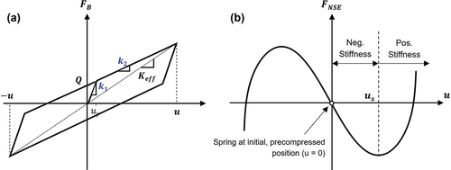
4.3. Nonlinearities at the Negative Stiffness Element ${\mathit{k}}_{\mathit{N}}$

Despite the assumptions made during the preliminary EKD design, the adopted NSE assembly is inherently nonlinear. As the NSE unit deforms, the precompressed spring extends, thus reducing its pre-compression force and the magnitude of the negative stiffness. The negative stiffness decrease eventually leads to positive spring stiffness at large displacements, resulting in the stiffening of the entire system. At this stage, the NSE no longer assists in vibration control but acts as a displacement restrainer for large earthquakes that may exceed the system’s design. Such behaviour is accounted for in the 3D FE model by assigning to the NSEs the force-displacement relationship of Fig. 8b (Attary et al. 2015a; Sarlis et al. 2013), where $u_s$ is the point of change from negative to positive stiffness for the precompressed spring. Following Sarlis et al. (2013), the force-displacement relationship will be:

(11) $F_{\mathit{NSE}}=-\left(\frac{F_p+K_s{L}_p}{l_s}-K_s\right)\left(\frac{l_1}{l_2}\right)\left(2+\frac{l_1}{l_2}+\frac{L_p+l_1}{\sqrt{{l_2}^2-u^2}}\right)\mathit{u}$(11)

where $\mathit{u}$ is the shear displacement of the NSE element and $l_s$ is derived from:

(12) $l_s=\sqrt{{\left[L_p+l_1+l_1\sqrt{1-{\left(\frac{u}{l_2}\right)}^2}\right]}^2+u^2{\left(1+\frac{l_1}{l_2}\right)}^2}$(12)

The values of critical parameters used to define the NSEs behaviour at the abutments and the pier are summarized in Table 5, including the undeformed length of the precompressed spring ($L_p$), the spring stiffness $K_s$, the pre-compression load $F_p$, and the lengths $l_1$ and $l_2$ (see also Fig. 3b).

Table 5. Values of parameters used to define the NSE behavior.

Parameters	$\mathit{EK}{\mathit{D}}_{\left(\mathit{i}=1\right)}\mathit{\hspace{0.17em}}$: Abutments*	$\mathit{EK}{\mathit{D}}_{\left(\mathit{i}=2\right)}\mathit{\hspace{0.17em}}$: Pier*
${\mathit{l}}_1:\mathit{m}$	0.2	0.2
${\mathit{l}}_2:\mathit{m}$	0.25	0.25
${\mathit{L}}_p:\mathit{m}$	0.5	0.5
${\mathit{k}}_s:\mathit{kN}/\mathit{m}$	180	110
Fp : kN	50	35

*The values correspond to individual NSEs per EKD at the abutments or the pier.

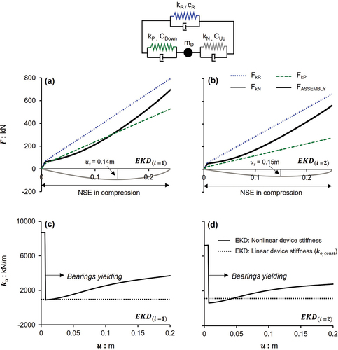
The exact force-displacement relationships adopted for the EKD components are illustrated in Fig. 9. More specifically, Fig. 9a,b plot the nonlinear force-displacement response of elements $k_R$, $k_P$ and $k_N$, as well as the resulting force of the EKD device, for $\mathit{EK}{D}_{\left(\mathit{i}\mathit{\hspace{0.17em}}=1\right)}$ and $\mathit{EK}{D}_{\left(\mathit{i}\mathit{\hspace{0.17em}}=2\right)}$ respectively. Figures 9c,d display the change in the device’s tangential stiffness $k_o=k_R+\frac{k_N{k}_P}{k_N+k_P}$, due to the nonlinearities of elements $k_P,k_R$ and $k_N$ (continuous black line). The curve is compared with the constant stiffness $k_{\mathit{o},\mathit{const}}$ assigned to the EKDs during preliminary design (dashed line). Initially, the overall stiffness is approximately three times larger than the one derived via the optimization process. At $\mathit{u}$ = 7.5 mm (i.e. the yield point of the bearings), the stiffness experiences a sudden drop towards the value calculated during the preliminary design. At that stage, the NSEs in both configurations ($\mathit{EK}{D}_{\left(\mathit{i}\mathit{\hspace{0.17em}}=1\right)}$ and $\mathit{EK}{D}_{\left(\mathit{i}\mathit{\hspace{0.17em}}=2\right)}$) work close to their initial negative stiffness. With increasing displacement, stiffening of the NSEs increases the overall stiffness of the EKD, which becomes almost twice as high as $k_{\mathit{o},\mathit{const}}$ at large displacements ($\mathit{u}$ = 0.20 m). As observed, the static stability of the EKD assembly is consistently maintained along the nonlinear force-displacement curve, evidenced by the positive values of the tangential stiffness $k_o\left(\mathit{u}\right)$. This is attributed to two primary factors:

Figure 9. Force – displacement response of the components and of the entire assembly: (a) $\mathit{EK}{D}_{\left(\mathit{i}=1\right)}$at the abutments; and (b) $\mathit{EK}{D}_{\left(\mathit{i}=2\right)}$ at the pier. Linear vs. nonlinear tangential stiffness $(k_o$) of: (c) $\mathit{EK}{D}_{\left(\mathit{i}=1\right)};$ and (d) $\mathit{EK}{D}_{(\mathit{i}=2)}$, considering nonlinearities in elements $k_P,k_R,k_N$.

1. The inherently low levels of nonlinearity present in the elastomeric bearings that serve as positive stiffness elements of the configuration ($k_R$, $k_P$): within the range of anticipated displacement values, the bearings display a controlled stiffness decrease, i.e. a single transition from stiffness $k_1$ to $k_2$=$k_1$/3.

2. The proper selection of elastomeric bearing properties, which ensures that the post-yielding bearing stiffness $k_2$ aligns with the $k_R$, $k_P$ values computed during the preliminary system design. This alignment implies that the lowest expected value of $k_o$, occurring upon bearing yielding, will remain close to the constant stiffness $k_{\mathit{o},\mathit{const}}$ assigned to the EKDs during the linear elastic design stage, thereby safely above zero.

4.4. Nonlinear Performance of the EKD System

The response of the bridge on EKDs, considering linear and nonlinear EKD components, is compared in Figs. 10 and 11. Results are displayed for the 2012 Emilia Romagna record (No. 10) and the 1986 El Salvador record (No.12), scaled according to Method B. The charts of Fig. 10b–d plot the drift time histories at the deck (${\delta }_{\mathit{Deck}}$), the $\mathit{EK}{D}_{\left(\mathit{i}\mathit{\hspace{0.17em}}=1\right)}$ mass (${\delta }_{\mathit{mD}1}$), and pier top (${\delta }_{\mathit{pier}}$), respectively. Two different comparisons are made to decouple the effect of nonlinearity at the bearings and the effect of stiffening at the NSE: (i) Case A: the bridge model with nonlinear $k_P$ and $k_R$ elements (grey lines) is compared to the system with linear EKDs (black lines); and (ii) Case B: the model with fully nonlinear EKDs ($k_P$, $k_R$, and $k_N$) is further compared to the previous (blue lines). It is noted that throughout the analyses, the bridge pier response is nonlinear.

Figure 10. Linear vs. nonlinear EKD response: (a) Acceleration spectra for the modified Emilia Romagna (2012) and El Salvador (1986) records (Method B), in comparison to the EC8 spectrum. Time histories of drift at: (b) the deck; (c) the $m_{\mathit{D}1}$ masses; and (d) the pier.

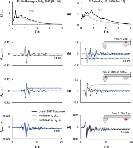
Figure 11. Time histories of deck acceleration for the modified Emilia Romagna and El Salvador records.

According to Fig. 10b, the nonlinearity of the elastomeric bearings (grey lines) leads to a slight decrease in maximum deck drifts under the examined records since the bearings absorb part of the seismic energy. However, this comes at the cost of permanent drifts. In the case of Emilia Romagna, ${\delta }_{\mathit{Deck},\mathit{res}}$ ≈1.5 cm, while for the stronger El Salvador (1986) record, ${\delta }_{\mathit{Deck},\mathit{res}}$ = 8.6 cm. It becomes apparent from Fig. 10c,d that the residual deck drift is a direct result of the nonlinear response of the bearings, as the EKD masses at the abutments also sustain a permanent drift. On the other hand, the bridge pier remains almost unaffected in Case A. Similarly to the linear case (black lines), it experiences insignificant levels of maximum drift (<1 cm) after both records. The trivial residual drift measured at the end of the El Salvador (1986) record (${\delta }_{\mathit{pier}}$ = 0.15 cm) is consistent in both the linear case and Case A, resulting from the significantly increased inertia forces exerted on the system (the spectrum of the motion lies above the EC8 spectrum, Fig. 10a).

An interesting behaviour is observed when the $k_N$ nonlinearity is introduced (blue lines): for the lower intensity Emilia Romagna record, where the NSEs work at their initial negative stiffness, the system performance is identical to that of Case A. On the contrary, under the increased displacements imposed by the El Salvador record, the NSEs undergo significant stressing, being forced to deform and reduce their negative stiffness. The resulting stiffening counterbalances the yielding experienced by the bearings, reducing the finally attained residual drift at the EKD masses (Fig. 10c,d, right). The permanent deck drift returns to zero (Fig. 10b, right), and the response closely resembles the elastic case. Pier response is unaffected.

As shown in Fig. 11, EKD nonlinearities only slightly decrease the maximum deck accelerations in both cases. At the same time, the Emilia Romagna record produces a noticeable increase in high-frequency acceleration amplitudes, a pattern that is not observed with the modified El Salvador record. It is concluded that the larger initial stiffness $k_1$ of the bearings (compared to the elastic EKD properties, where the bearings’ stiffness equals $k_2$) excites high-frequency ground shaking, which amplifies deck accelerations for the higher frequency Emilia Romagna record.

4.5. Nonlinear EKD Vs Nonlinear CSI

To verify the efficiency of the nonlinear EKD concept against the CSI, transient time history analyses are performed, employing the Method B suite of ground motions and two nonlinear 3D bridge configurations: (i) the initial system on isolation bearings (CSI); and (ii) the isolated bridge on EKDs (EKD). The simulation of the hysteretic response of the CSI bearings follows the same methodology described for the positive EKD elements. At 100% shear strain, the damping of the bearings is calculated approximately equal to ${\xi }_{\mathit{eff}}$ = 5%, based on Eq. (8)(8) ${\xi }_{\mathit{eff}}=\frac{4\mathit{Q}\left(\mathrm{u}-\mathit{\hspace{0.17em}}{\mathrm{u}}_{\mathrm{y}}\right)}{2\mathit{\pi }{\mathrm{K}}_{\mathrm{eff}}\mathit{\hspace{0.17em}}{\mathrm{u}}^2}$(8) .

The performance of the system is presented in terms of maximum and residual deck drifts, deck accelerations, and peak base shear versus Arias Intensity $I_A$ (Arias 1970) in Fig. 12. Recognized as a fairly reliable Intensity Measure (IM), the latter is often used individually or in combination with other IMs for the assessment of the damage potential of nonlinear systems to seismic excitations (e.g. Anastasopoulos et al. 2015). It is noted that the base shear equals the shear force transferred from the deck to the bridge pier. The Arias Intensity is plotted on the horizontal axis, while the seismic record number is also noted on the graphs for ease of reference. The performance under low amplitude earthquakes (No. 1–7) is not examined.

Figure 12. EKD_nonlinear vs CSI_nonlinear under Method B records: (a) maximum deck drift; (b) residual deck drift; (c) maximum deck accelerations; and (d) peak base shear versus Arias Intensity $\left(I_A\right)$.

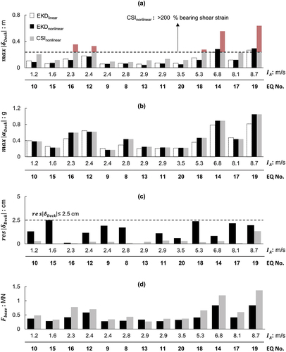
Besides offering a direct comparison between the nonlinear EKD and CSI systems, Fig. 12 also summarises the effect of nonlinearities on the EKD system under the ensemble of Method B motions (EKD_linear vs EKD_nonlinear). Notably, for excitations No. 14, 15 and 19 (as depicted in Fig. 12a), there is no decrease in maximum deck drifts for the EKD_nonlinear due to the nonlinearity of the elastomeric bearings; instead, there is an increase in comparison to the EKD_linear. This contrasts with the observations from Fig. 10 and can be attributed to the varying ground motion characteristics and their correlation to the period of the nonlinear structure at the imposed displacement amplitude, further emphasizing the significance of using seismic motions of diverse characteristics in the design process. Nevertheless, the increase does not exceed 20% for all examined records. A similar conclusion is derived from the comparison of maximum deck accelerations between the EKD_linear and EKD_nonlinear systems in Fig. 12b (black vs white bars).

The dependence of system performance on seismic frequency is also apparent in the response under increasing Arias Intensities. It becomes evident that $I_A$ alone cannot serve as a reliable proxy for the assessment of damage potential (i.e. high values of $I_A$ do not necessarily produce higher maximum displacements) because the correlation between earthquake and system fundamental frequencies largely drives the system’s inertial response.

The EKD_nonlinear model is subsequently compared to the CSI_nonlinear (Fig. 12a–d). The results confirm the superiority of EKD_nonlinear in terms of maximum deck drifts (Fig. 12a). Similarly to what was presented earlier, the nonlinear CSI develops large maximum deck drifts during records No. 12, 14, 16, 18, and 19, which lead to prohibitive shear strains at the isolation bearings (i.e. bearing failure). On the contrary, the bearing deformations for the EKD_nonlinear system remain below the threshold of ${\epsilon }_s$ < 200%, even under the very high amplitude of the modified Takatori 000 record (Kobe, Japan, 1995). Moreover, the EKD_nonlinear seems to effectively reduce the maximum base shear $F_{\mathit{base}}$ for most ground motions (Fig. 12d), with the maximum decrease being observed for the modified Kobe record (38%).

Contrary to what was presented in Fig. 6 (linear elastic dynamic analyses), the EKD_nonlinear and CSI_nonlinear systems exhibit similar responses in terms of maximum deck accelerations (Fig. 12b). This is partly due to the hysteretic response of the CSI bearings, which to some extent reduces the deck accelerations of the CSI_nonlinear system, and partly due to the higher accelerations experienced by the EKD_nonlinear compared to the linear case, stemming from the stiffening of the NSEs at large displacements. The response is deemed satisfactory, as the proposed concept retains the benefit of reduced accelerations – typical of conventional seismic isolation systems – while concurrently eliminating their primary disadvantage by suppressing excessive displacements. Two potential strategies could be implemented to further diminish deck accelerations: introducing additional damping to the EKD devices or redesigning the EKDs to delay their stiffening behaviour, thereby maintaining negative stiffness across a broader range of deformations.

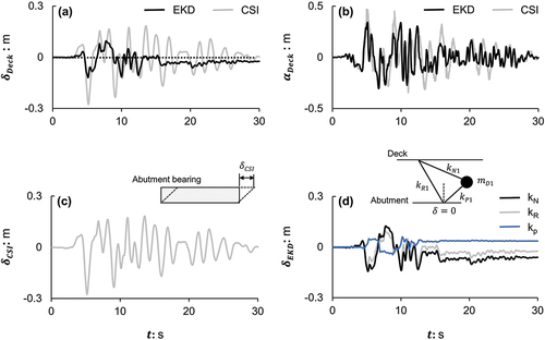
According to Fig. 12c, the EKDs result in permanent relative deck displacements $\mathit{res}\left|{\delta }_{\mathit{Deck}}\right|$ for almost all examined motions, which nevertheless remain below 2.5 cm. The observed behaviour is less prevalent in the case of the CSI_nonlinear, although in most cases, the bearings are operating well beyond their yield limit. Figure 13 elaborates on this phenomenon using results from record No. 18 (Kocaeli, Turkey, 1999). Owning to the “symmetric” nature of the motion (similar acceleration amplitudes at positive and negative directions, as observed in Fig. 13b), the deck returns to its initial position at the end of shaking in the case of CSI_nonlinear (Fig. 13a), following the relative movement of the bearings (Fig. 13c). The deformation of individual EKD elements, however, is more complicated (Fig. 13d). The additional mass ($m_D$) moves out of phase with the deck, causing opposing displacements to the negative ($k_N$) and positive ($k_P$) device elements. The absolute difference between these displacements equals the drift of the $k_R$ element and, subsequently, the deck. The incurring nonlinearities yield permanent drifts of dissimilar amplitude in the device elements, forcing the additional mass towards a new equilibrium point of $\mathit{\delta }\ne$ 0 at the end of shaking and the deck to a permanent drift.

Figure 13. EKD_nonlinear vs. CSI_nonlinear under the modified Kocaeli record (No.18). Time histories of: (a) deck drift; (b) deck acceleration; (c) relative displacement of CSI abutment bearings; and (d) relative displacement of $\mathit{EK}{D}_{\left(\mathit{i}=1\right)}$ elements.

As illustrated in Fig. 14, this new equilibrium point is controlled by the residual drift of the negative stiffness element, which may take values in the range of 0 to $u_s$ (i.e. the displacement where the precompressed spring stiffness changes from negative to positive). The figure plots the drift time history (${\delta }_{\mathit{kN}}$) of the $\mathit{EK}{D}_{\left(\mathit{i}\mathit{\hspace{0.17em}}=1\right)}$negative stiffness element under one sinusoidal cycle of increasing load amplitude $\mathit{F}$, expressed as a percentage of the $\mathit{EK}{D}_{\left(\mathit{i}\mathit{\hspace{0.17em}}=1\right)}$ system yield force $F_{\mathit{yield}}$ (Fig. 14a). The results indicate that for load amplitudes closer to the yield force (e.g. $\mathit{F}/F_{\mathit{yield}}$ = 3) the residual drift ${\delta }_{\mathit{kN}},\mathit{res}$ < $u_s$. As the force amplitude (and, therefore, the incurring nonlinearity) increases, ${\delta }_{\mathit{kN}},\mathit{res}$ $\to u_s$, yet without surpassing this threshold even for large magnitudes of applied dynamic load. It is interesting to observe that for the same amplitude of applied load, the finally attained residual drift is sensitive to the natural period of loading (Fig. 14b); periods lying closer to the fundamental $\mathit{EKD}$ fundamental period lead to lower permanent drifts for the $k_N$ element and subsequently for the system, owing to the $\mathit{EKD}$ being designed to optimize performance within that region of loading frequencies.

Figure 14. (a) Drift time histories ${\delta }_{\mathit{kN}}$ of the negative $\mathit{EK}{D}_{\left(\mathit{i}=1\right)}$ element subjected to sinusoidal loading of various amplitudes; and (b) correlation of residual negative stiffness ${\delta }_{\mathit{kN},\mathit{res}}$ with $\mathit{F}/F_{\mathit{yield}}$ for two different loading frequencies.

It is acknowledged that the absence of abutment stoppers at the model edges affects the seismic performance assessment of the structure, both in the case of the EKD_nonlinear and the CSI systems. For the latter, modelling the stoppers in the longitudinal direction would restrain the deformation of the bearings below code limits and allow re-distribution of damage in the structure. Most importantly, however, the response of the EKD devices could be affected as the deck of the EKD system collides with the stoppers. This very effect is examined in the last section of the paper.

5. The Effect of SSI

This section employs a more detailed 3D FE model of the entire soil – foundation–structure system to investigate the role of SSI. One case of a strong motion is examined (modified Takatori 000 record, Method B), where the abutment stoppers are activated, and the effects of SSI are highlighted.

5.1. Numerical Modelling: Soil, Foundation, and Abutments

In the FE model of Fig. 15, the soil domain is simulated with nonlinear continuum (brick) elements (C3D8). The nonlinear response of clay is modelled with a kinematic hardening constitutive model that follows the Von Mises failure criterion with associated flow rule. The model formulation is available in Abaqus and has been parameterized by Anastasopoulos et al. (2011) to simulate the monotonic and cyclic response of clays and sands. Despite its simplicity, the model has been extensively validated against physical model tests of surface and embedded foundations (Anastasopoulos et al. 2011), piles and caissons (Giannakos et al. 2012; Zafeirakos et al. 2013), proving its efficiency in capturing the soil – foundation response. For the full description of the nonlinear clay response, only three parameters need to be determined: the undrained shear strength $S_u$, the ratio $E_o$/$S_u$ (refer to Section 2), and $\mathit{\gamma }$, a scalar coefficient that determines the rate of decrease of kinematic hardening with increasing plastic deformation.

Figure 15. (a) 3D FE model of the entire soil – foundation–structure system; and (b) cut view with the pile group foundation being highlighted.

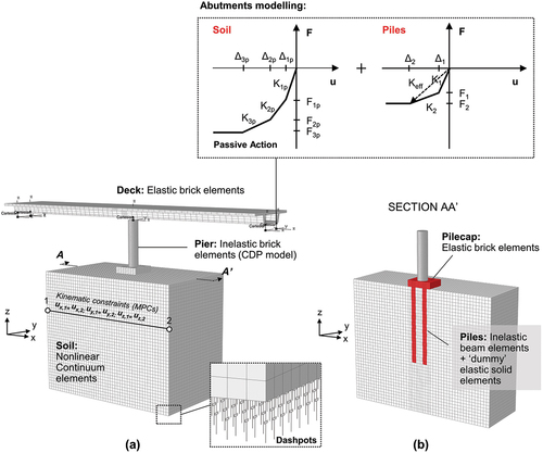
The concrete pile cap is simulated with elastic continuum elements of Young’s modulus $\mathit{E}$ = 30GPa. The piles are simulated by employing a hybrid modelling technique, where central nonlinear beams are used to simulate the moment-curvature response of the RC piles (obtained from section analysis assuming 1% reinforcement ratio). The beams are embedded in 3D continuum elements of almost zero stiffness (“dummy” elements) that enable a realistic representation of the pile periphery. Tensionless contact elements are introduced at the soil-pile interfaces to model potential separation and sliding, while a friction coefficient $\mathit{\mu }$ = 0.35 is assumed between the soil and the piles. Soil radiation damping is taken into account by introducing appropriate absorbing boundaries at the base of the model. The dashpot coefficient is calculated as:

(13) $C_b=\mathit{\rho }{V}_s\mathit{A}$(13)

where: $\mathit{\rho }$ = 2 Mg/m³ is the clay density, V_s is the shear wave velocity corresponding to half-space, and A is the effective area of each dashpot. Moreover, “node-to-node” kinematic constraints (MPCs) are applied along the soil boundaries parallel to the y-axis, forcing two nodes to have identical displacements. Such an approach aims to simulate the response of a soil column subjected to in-plane vertically propagating waves. Displacements at the bottom dashpot nodes are constrained ($u_x=u_y=u_z=0$), as are the vertical displacements ($u_z$) of the soil base (i.e. the top dashpot nodes) and the out-of-plane displacements ($u_y$) of the soil boundaries parallel to the x-axis.

Appropriate gap elements are introduced at the edges of the bridge to replicate the ${\delta }_c$ = 100 mm clearance between the deck and the abutment stoppers. The stoppers are engaged when the available clearance is consumed, impeding the lateral deck movement. In this way, they effectively limit the deck drift while protecting the bearings from excessive shear strain. The bridge abutments are modelled simplistically, with nonlinear 1D hysteretic truss elements that simulate their resistance. The truss elements follow a kinematic hardening constitutive model with Von Mises failure criterion and associated flow rule, such as the one adopted for the soil. Both the backfill soil and the abutment piles contribute to the passive resistance of the abutment. The nonlinear force-displacement abutment behaviour is derived from a combination of design recommendations (Caltrans 1990, 1999) and experimental results on seat-type abutments with piles (Maroney et al. 1993). Figure 15 depicts the adopted analytical model, breaking it down into nonlinear force-displacement curves that represent the contribution of the soil and piles, respectively. The initial soil stiffness ($K_{1\mathit{p}}$ in Fig. 15) and ultimate resistance ($F_{3\mathit{p}}$ in Fig. 15) are expressed as functions of the abutment wall dimensions as follows:

(14) $K_{1\mathit{p}}=a_1\mathit{w}$(14)

(15) $F_{3\mathit{p}}={\mathit{H}}_w\mathit{w}{p}_1$(15)

where: $\mathit{w}=11$m is the wall width, ${\mathit{H}}_w$ = 7.5 m is the wall height, $a_1$ = 20.2 KN/mm/m is the unit initial soil stiffness (Caltrans 1999), and $p_1$ = 370 kPa is the ultimate soil pressure (Caltrans 1999). The ultimate soil resistance $F_{3\mathit{p}}$ is reached at a relative displacement of ${\mathrm{\Delta }}_{3\mathit{p}}$ = 0.1${\mathit{H}}_w$, while the yield displacement is set at ${\mathrm{\Delta }}_{1\mathit{p}}$ = 0.1${\mathrm{\Delta }}_{3\mathit{p}}$ and ${\mathrm{\Delta }}_{2\mathit{p}}$ = 0.35${\mathrm{\Delta }}_{3\mathit{p}}$. Following Caltrans (1990), the effective horizontal stiffness of the piles is assumed to be equal to $K_{\mathit{eff}}$ = 7 kN/mm/pile, while the ultimate pile strength is set to $F_2$ = 119 kN/pile (refer to Fig. 15). The individual stiffnesses $K_1$, $K_2$ and displacements ${\mathrm{\Delta }}_1$, ${\mathrm{\Delta }}_2$ of the tri-linear pile curve are calculated as functions of $K_{\mathit{eff}}$ and $F_2$. The adopted abutment model is described in further detail in the work of Nielson (2005).

5.2. Response of the EKD System to the Modified Takatori Record (Kobe, Japan, 1995)

The section compares the performance of the bridge with EKDs subjected to the modified Takatori 000 record from Kobe, Japan, 1995 (No. 19), with and without the incorporation of abutment stoppers. The analysis is conducted through a sequence of steps. After applying the geostatic soil stresses (Step 1) and the dead loads of the foundation and superstructure (Step 2), the model undergoes a dynamic analysis step, wherein seismic acceleration is applied at the model base along the x-axis.

The key results are summarized in Figs. 16 and 17. Figure 16 displays the plastic strain contours at the end of shaking for the model that ignores the abutment stoppers. The plastic strains in the soil around the piles reveal non-trivial SSI effects, contrary to what was initially assumed. These effects become more pronounced due to the intensity of the seismic motion (which is the strongest of the ones considered), which is amplified further (by approximately 15%) while propagating through the clay medium.

Figure 16. Soil – foundation–structure model subjected to the modified Takatori record (Kobe, Japan, 1995), ignoring the contribution of abutment stoppers: (a) contours of plastic strains (PEMAG) at the end of shaking; and (b) close-up of pier tensile damage (DAMAGET), also at the end of shaking.

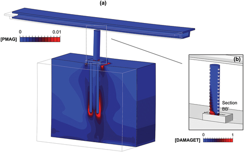
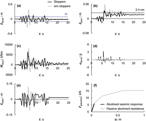
Figure 17. Comparison of the 3D soil – foundation–structure model subjected to the modified Takatori record, with and without stoppers. Time histories of: (a) deck drift; (b) pier drift; (c) bending moment of section BB’; (d) deck acceleration; and (e) drift of the $m_{\mathit{D}1}\mathit{\hspace{0.17em}}$ mass. In (f), the seismic response of the right abutment (in black) is compared to the passive abutment resistance (grey dotted line).

The larger accumulation of strain at the right side of the pile cap indicates that the pier – foundation system sustains permanent deformation towards that side, a fact also confirmed by the 2.4 cm of residual pier drift that can be seen in the time history of Fig. 17b (grey line). Such behaviour is naturally not captured by the simplified model of Section 3, which assumes an elastic soil-foundation response. The permanent pier drift is accompanied by increased pier stressing, as revealed by the tensile damage contours at its base and lower-left side (Fig. 16b). SSI has a measurable effect on deck response, but to a smaller extent. The maximum deck drift is increased by roughly 22% compared to the prediction of the simplified model of Section 3 (0.37 m vs. 0.29 m in Fig. 12a, for record No. 19), implying a slightly inferior performance.

Figure 17 compares the response of the 3D model with and without stoppers. The small available clearance ${\delta }_c$ = 100 mm is consumed already during the first strong motion cycles, where the deviations in deck drift between the two models begin (Fig. 17a). Upon collision with the deck, the abutments deform, and therefore the relative deck displacement is not strictly restrained to 100 mm. During the increased amplitude cycles that follow, the deck keeps pounding on the stoppers, reducing its maximum relative displacement to 150 mm, compared to 370 mm without stoppers. Due to this considerable deck drift reduction, the maximum and residual pier drifts are also reduced (Fig. 17b), decreasing pier bending moments throughout shaking (Fig. 17c).

Alas, the beneficial effect on system drifts comes at the expense of significantly enlarged deck accelerations (Fig. 17d). Every time the deck pounds on the abutments, the impact is translated to acceleration spikes in the time history of $a_{\mathit{Deck}}$, with values three times higher than in the absence of stoppers (possibly large enough to induce structural damage to the deck). Moreover, it is interesting to observe that the deck collision to the abutments essentially inhibits the operation of the EKDs (Fig. 17e), dropping the maximum drifts experienced by the mass $m_{\mathit{D}1}$ by over 50% and producing residual EKD displacements (${\delta }_{\mathit{mD}1,\mathit{res}}$ = 1.5 cm). Throughout the analysis, the seismic demand on the abutments does not exceed the yielding point in the relevant force – displacement curve (Fig. 17e), indicating trivial damage due to deck pounding.

6. Summary, Conclusions & Limitations

The study performed a numerical investigation of the seismic performance of a benchmark bridge isolated with a novel vibration isolation and damping device termed Extended KDamper (EKD). The benchmark system is a representative single-pier RC bridge, initially designed with conventional seismic isolation (CSI) on elastomeric bearings. The key conclusions of the study can be summarized as follows:

• The study has highlighted the need to incorporate earthquake motion characteristics in the design process of the EKD to ensure the effectiveness of the isolation system for a wide range of input seismic motions.

• The comparison of the bridge with CSI and EKDs via elastic dynamic analysis demonstrates a significant decrease in deck displacements upon the incorporation of the EKDs. Specifically, the EKDs achieve a reduction in deck drifts ranging from 40% to 70% across the examined seismic motions. Unlike the CSI system, which was found to sustain excessive bearing shear strains when exposed to the most severe excitations of the set, the EKD system’s bearings never surpassed the 200% threshold. On average, the EKDs also outperformed the CSI in terms of deck accelerations, albeit to a smaller extent compared to deck displacements.

• Nonlinear 3D dynamic time history analyses (where the hysteretic response of the elastomeric bearings and the nonlinear nature of the negative stiffness elements were explicitly simulated) demonstrated that the nonlinearities in the positive stiffness elements of the EKD ($k_P,k_R$) may lead to residual deck drifts, which on several occasions were counterbalanced by the stiffening of the NSE ($k_N)$ in large displacements. The changing stiffness of the EKDs implies that the seismic performance of the isolation system depends on the characteristics of the ground motion.

• For the evaluated spectrum-compatible records, the nonlinear EKDs exhibit a variation in maximum drifts and accelerations approximately within the range of ±20% compared to the preliminary (linear elastic) design. The observed increase in accelerations is attributed to the stiffening of the NSEs, and as such, it is more pronounced for seismic motions with larger displacement demands.

• A direct comparison of the bridge on nonlinear EKDs and nonlinear CSI confirms the superior performance of the EKDs in terms of deck drifts, bearing shear strains, and base shear. The use of EKDs may allow for a more economical design of the pier in the case of a new bridge. Nevertheless, the response of the original CSI system is better in terms of permanent deck displacements, while the two systems were found to be equivalent in terms of maximum deck accelerations.

• With the aid of a fully nonlinear 3D FE model of the entire soil – foundation–structure system, SSI effects were shown to have a significant impact on the overall seismic response of the system. The deck’s collision with the abutments reduced the maximum attained deck drift and relative residual pier displacement; however, it was shown to compromise the performance of the EKDs, leading to a substantial increase in deck accelerations.

The following study limitations are recognized and are outlined herein as recommendations for future work:

1. The obtained numerical results are specific to the examined benchmark bridge and cannot be generalized. Further analyses would be required for a variety of bridge configurations to safely derive the improved performance margins of the EKD versus conventional isolation systems.

2. The simplified mathematical model of the bridge on EKDs calls for further improvements. The 1-D model does not account for the nonlinear behaviour of structural elements and EKDs or SSI effects. Moreover, the model neglects the effects of torsion potentially arising from disparities in the properties of the different EKD devices, an effect that should be further explored in future studies.

3. Future research endeavours could benefit from the explicit simulation of the abutments and the negative stiffness element as a precompressed mechanical spring in a 3D FE environment.

4. The device’s performance under two-directional seismic shaking should be thoroughly evaluated to ascertain the technical robustness of its application to bridge structures.

Notation

$C_b$ :	=	dashpot coefficient
$C_{\mathit{up}},C_{\mathit{down}}$ :	=	damping factors of the EKD device
$E_{\mathit{comp}}$ :	=	instantaneous compression modulus of the rubber-steel composite under specified level of vertical load in elastomeric bearings
$E_o$ :	=	small-strain elastic modulus of soil
$E_p$ :	=	pile elastic modulus
$E_s$ :	=	steel Young’s modulus
$F_{3\mathit{p}}$ :	=	ultimate abutment soil resistance
$F_{\mathit{base}}$ :	=	maximum base shear
$F_p$ :	=	mechanical spring precompression load
$K_{1\mathit{p}}$ :	=	initial abutment soil stiffness
$K_{\mathit{b},\mathit{H}}$ :	=	horizontal stiffness of elastomeric bearing
$K_{\mathit{b},\mathit{V}}$ :	=	vertical stiffness of elastomeric bearing
$K_c$ :	=	concrete damage plasticity model parameter
$K_s$ :	=	mechanical spring stiffness
$K_{\mathit{tot}}:$	=	total bridge stiffness
$L_p$ :	=	undeformed length of the precompressed mechanical spring
$S_u$ :	=	undrained shear strength
$T_E$ :	=	fundamental earthquake period
$T_n$ :	=	bridge fundamental natural period
$V_s$ :	=	soil shear wave velocity
$a_1$, $p_1$ :	=	coefficients employed in the calculation of abutment soil stiffness and ultimate resistance
$c_D$ :	=	damping factor of the K-Damper device
$c_s$ :	=	damping factor of a structural system
$d_s$ :	=	bearing drift
$f_{\mathit{ck}}$ :	=	characteristic concrete compressive strength
$f_t$ :	=	concrete tensile strength
$f_y$ :	=	steel yield strength
$k_1$ :	=	initial stiffness in the bilinear law characterizing elastomeric bearings behaviour
$k_2$ :	=	post-yielding stiffness in the bilinear law characterizing elastomeric bearings behaviour
$k_N$ :	=	negative stiffness element of the K-Damper (or EKD) device
$k_P$ :	=	positive stiffness element of the K-Damper (or EKD) device
$k_R$ :	=	positive stiffness element working in parallel with the EKD device
$k_b$ :	=	elastomeric bearing stiffness
$k_o$ :	=	tangential stiffness of the EKD device
$k_{\mathit{pier}}$ :	=	pier stiffness
$l_1$, $l_2$ :	=	lengths on the NSE device, used as input for the calculation of the NSE force-displacement relationship
$m_D$ :	=	additional mass of the K-Damper (or EKD) device
$m_{\mathit{deck}}$ :	=	deck mass
$m_{\mathit{pier}}$ :	=	pier mass
$m_s$ :	=	mass of bridge deck
$t_r$ :	=	height of elastomer layer
$u_s$ :	=	point of change from negative to positive stiffness for the precompressed spring (displacement value)
$u_y$ :	=	bearing yield displacement
$x_{\mathit{deck}},x_{\mathit{pier}},x_{\mathit{G},}{x}_{\mathit{D}1,}{x}_{\mathit{D}2}:$	=	horizontal displacements of the bridge deck, pier top, structure base, and of the additional EKD masses
${\mathrm{H}}_w$ :	=	abutment wall height
${\mathrm{K}}_{\mathit{eff}}$:	=	bearing effective stiffness
${\delta }_c$ :	=	clearance between the deck and the abutment stoppers
${\delta }_{\mathit{pier},\mathit{res}}$ :	=	residual pier drift
${\delta }_{\mathit{pier}}$ :	=	pier drift
${\epsilon }_N$, ${\epsilon }_P$ and ${\epsilon }_R$ :	=	variations in the positive and negative stiffness elements of the EKD devices
${\epsilon }_s$ :	=	seismic shear strain
${\xi }_{\mathit{eff}}$ :	=	effective damping ratio
${\sigma }_{\mathit{bo}}/{\sigma }_{\mathit{co}}$ :	=	concrete damage plasticity model parameter
$\mathit{A}$ :	=	Area
$\mathit{BW}$ :	=	bandwidth
$\mathit{CSI}$ :	=	Conventional seismic isolation
$\mathit{D}$ :	=	pier diameter
$\mathit{E}$ :	=	concrete Young’s modulus
$\mathit{G}$ :	=	shear modulus
$\mathit{H}$ :	=	height
$\mathit{H}$ :	=	pier height
$\mathit{HMCR}$ :	=	harmony consideration rate
$\mathit{HMS}$ :	=	harmony memory size
$\mathit{L}$ :	=	length
$\mathit{L}:$	=	pile length
$\mathit{MaxItr}$ :	=	maximum iteration number
$\mathit{PAR}$ :	=	pitch adjusting rate
$\mathit{PGA}$ :	=	Peak Ground Acceleration
$\mathit{Q}$ :	=	characteristic bearing strength
$\mathit{S}$ :	=	bearing shape factor
$\mathit{W}$ :	=	width
$\mathit{d}$ :	=	pile diameter
$\mathit{max}\left|a_{\mathit{Deck}}\right|$ :	=	maximum absolute deck acceleration
$\mathit{max}\left|{\delta }_{\mathit{Deck}}\right|$ :	=	maximum absolute deck drift
$\mathit{res}\left|{\delta }_{\mathit{Deck}}\right|$ :	=	residual (absolute) deck drift
$\mathit{s}$ :	=	distance between foundation piles
$\mathit{u}$ :	=	horizontal displacement
$\mathit{u},\dot{u},\ddot{u}$ :	=	relative displacement (drift), velocity & acceleration in the presented equations of motion
$\mathit{w}$ :	=	abutment wall width
$\mathit{\gamma }$ :	=	scalar coefficient that determines the rate of decrease of kinematic hardening with increasing plastic deformation in the employed soil constitutive model
$\mathit{\mu }$ :	=	friction coefficient
$\mathit{\nu }$ :	=	Poisson’s ratio
$\mathit{\xi }$ :	=	Rayleigh damping ratio
$\mathit{\rho }$ :	=	material density
$\mathit{\psi }$ :	=	concrete dilation angle
$\mathit{ϵ}$ :	=	flow potential eccentricity

Acknowledgments

This work was financially supported by the European Union’s Horizon 2020 research and innovation programme under the Marie Skłodowska-Curie grant agreement No INSPIRE-813424. The first author would like to thank Dr Athanasios Agalianos (ETH Zurich, Switzerland) and Mr Antonios Mantakas (NTUA, Greece) for the fruitful discussions and constructive criticism over the course of this research.

Disclosure Statement

No potential conflict of interest was reported by the author(s).

Data Availability Statement

The data that support the findings of this study are available from the corresponding author, Ioanni Anastasopoulo, upon reasonable request.

Additional information

Funding

This work was supported by the H2020 Marie Skłodowska-Curie Actions [INSPIRE-813424].

Notes

1. https://peer.berkeley.edu/peer-strong-ground-motion-databases.

Appendix A:

Equations of motion for the linear 2-DoF model of the bridge on CSI

The equations of motion of the 2-DoF model representing the bridge on CSI subjected to ground acceleration ${\ddot{x}}_{\mathit{G}}\left(\mathit{t}\right)$ are formulated as follows:

(A1) $\left[\begin{array}{cc}{m}_{\mathit{pier}}& 0\\ 0& m_{\mathit{deck}}\end{array}\right]\left[\begin{array}{c}{\ddot{u}}_{\mathit{pier}}(\mathit{t})\\ {\ddot{u}}_{\mathit{deck}}(\mathit{t})\end{array}\right]+\left[\begin{array}{cc}{c}_{\mathit{pier}}+c_{\mathit{b}2}& -c_{\mathit{b}2}\\ -c_{\mathit{b}2}& c_{\mathit{b}1}+c_{\mathit{b}2}\end{array}\right]\left[\begin{array}{c}{\dot{u}}_{\mathit{pier}}(\mathit{t})\\ {\dot{u}}_{\mathit{deck}}(\mathit{t})\end{array}\right]+\left[\begin{array}{cc}{k}_{\mathit{pier}}+k_{\mathit{b}2}& -k_{\mathit{b}2}\\ -k_{\mathit{b}2}& k_{\mathit{b}1}+k_{\mathit{b}2}\end{array}\right]\left[\begin{array}{c}{u}_{\mathit{pier}}(\mathit{t})\\ u_{\mathit{deck}}(\mathit{t})\end{array}\right]=-\left[\begin{array}{cc}{m}_{\mathit{pier}}& 0\\ 0& m_{\mathit{deck}}\end{array}\right]{\mathbf{1}}_r^T{\ddot{\mathrm{x}}}_{\mathrm{G}}(\mathrm{t})$(A1)

where

• $u_{\mathit{deck}}\left(\mathit{t}\right)$ = $x_{\mathit{deck}}\left(\mathit{t}\right)$ - $x_G\left(\mathit{t}\right)$, $u_{\mathit{pier}}\left(\mathit{t}\right)$ = $x_{\mathit{pier}}\left(\mathit{t}\right)$ - $x_G\left(\mathit{t}\right)$ are the deck and pier drifts, respectively.

• $k_{\mathit{b}1}=4\times k_b$ = 10920 kN/m and $k_{\mathit{b}2}=k_b=2730\mathit{kN}/\mathit{m}$ represent the total stiffness of the abutment and pier bearings, respectively.

• $c_{\mathit{pier}}$, $c_{\mathit{b}1}$, and ${\mathrm{c}}_{\mathrm{b}2}\mathit{\hspace{0.17em}}$ are the damping coefficients of the pier, abutment bearings and pier bearing, respectively, calculated under the assumption of mass and stiffness proportional damping, using the same damping ratio in both eigenmodes ($\mathit{\xi }$ = 5%, considered representative of both the reinforced concrete pier and the isolation bearings, following the suggestion of Bollano, Kapasakalis, and A 2021).

• ${{\mathbf{1}}_{\mathit{r}}}^{\mathit{T}}$ is an $\mathit{r}$x$1$ vector of ones, with $\mathit{r}$ = 2 (influence vector in the case of horizontal, one-dimensional, ground motion).

Appendix B:

Harmony search optimization algorithm

The four basic steps of the HS algorithm are briefly provided below. A more detailed algorithm description may be found in Geem et al. (2001) or Nigdeli and Bekdaş (2017).

Step 1: Initialization of the HS Memory matrix ($\mathit{HM}$). HM matrix contains vectors that represent possible solutions to the examined optimization problem. The initial $\mathit{HM}$ matrix is populated with randomly generated solution vectors, laying within user-defined boundaries for each independent design variable. The number of these vectors is determined by the Harmony Memory Size (HMS), and hence, for an $\mathit{n}$-dimension problem (where $\mathit{n}$ is the number of independent design variables), $\mathit{HM}$ obtains the following form:

(B1) $\mathit{HM}=\left[\begin{array}{c}{x_1}^1,{x_2}^1,\dots ,{x_n}^1\\ {x_1}^2,{x_2}^2,\dots ,{x_n}^2\\ .\\ .\\ .\\ {x_1}^{\mathit{HMS}},{x_2}^{\mathit{HMS}},\dots ,{x_n}^{\mathit{HMS}}\end{array}\right]$(B1)

where $[{x_1}^{\mathit{i}},{x_2}^{\mathit{i}},\dots ,{x_n}^{\mathit{i}}$] with $\mathit{i}$ = 1, 2, … , $\mathit{HMS}$ is a solution candidate. In this study, HMS is set to 75. For every solution vector, the algorithm calculates the value of the objective function.

Step 2: Improvisation of a new solution vector $\left[x_1^{\prime },x_2^{\prime },\dots ,x_n^{\prime }\right]$]. The creation of this new vector is largely driven by two principal parameters: the Harmony Memory Considering Rate ($\mathit{HMCR}$) and the Pitch Adjusting Rate ($\mathit{PAR}$). The $\mathit{HMCR}$ represents the probability that a component of the new solution vector will be selected from existing members in the Harmony Memory ($\mathit{HM}$). In contrast, the probability of generating a completely new component, that is, a value not currently present in the $\mathit{HM}$, is given by (1 – $\mathit{HMCR}$). This dichotomy allows for a balance between exploiting known good solutions (those in the $\mathit{HM}$) and exploring new potential solutions (randomly generated). When a component is chosen from the $\mathit{HM}$ matrix, an additional decision is made based on the $\mathit{PAR}$, which represents the probability that the chosen component will undergo a pitch adjustment, or mutation. The range of the adjustment is determined by the bandwidth $\mathit{BW}$. This step introduces further variation in the search space and enables a finer-grained search around known good solutions. In this study, $\mathit{HMCR}$ = 0.5, $\mathit{PAR}$ = 0.1 and $\mathit{BW}$ = 0.5.

Step 3: Update of the $\mathit{HM}$ matrix. The value of the objective function of the new solution, obtained in Step 2, is calculated and compared to the ones that correspond to the original $\mathit{HM}$ matrix vectors. If it results in better fitness than that of the worst member in the $\mathit{HM}$, it will replace it. In the typical case of a minimization optimization process, the new solution replaces a member of the $\mathit{HM}$ matrix only if that member has a bigger objective function value than the new one. If there is more than one member in the $\mathit{HM}$ with larger values of the objective function than the new solution, the one with the higher value is replaced. Otherwise, the new solution is eliminated, and the $\mathit{HM}$ matrix remains intact.

Step 4: Repetition of Steps 2 and 3 until a preset termination criterion is met. A commonly used termination criterion is the maximum number of total iterations, which in our study is set to $\mathit{MaxItr}$ = 1000.

References

- Alfarah, B., F. López-Almansa, and S. Oller. 2017. New methodology for calculating damage variables evolution in plastic damage model for RC structures. Engineering Structures, Elsevier Ltd 132:70–86. doi:10.1016/j.engstruct.2016.11.022.
- Anastasopoulos, I., P. C. Anastasopoulos, A. Agalianos, and L. Sakellariadis. 2015. Simple method for real-time seismic damage assessment of bridges. Soil Dynamics and Earthquake Engineering 78:201–12. doi:10.1016/j.soildyn.2015.07.005.
- Anastasopoulos, I., F. Gelagoti, R. Kourkoulis, and G. Gazetas. 2011. Simplified constitutive model for simulation of cyclic response of shallow foundations: Validation against laboratory tests. Journal of Geotechnical and Geoenvironmental Engineering 137 (12):1154–68. doi:10.1061/(ASCE)GT.1943-5606.0000534.
- Antoniadis, I. A., S. A. Kanarachos, K. Gryllias, and I. E. Sapountzakis. 2016. Kdamping: A stiffness based vibration absorption concept. Journal of Vibration and Control 24 (3):588–606. doi:10.1177/1077546316646514.
- Antoniadis, I. A., K. A. Kapasakalis, and E. J. Sapountzakis. 2019. Advanced negative stiffness absorbers for the seismic protection of structures. doi:10.1063/1.5123704.
- Antoniou, M., N. Nikitas, I. Anastasopoulos, and R. Fuentes. 2020. Scaling laws for shaking table testing of reinforced concrete tunnels accounting for post-cracking lining response. Tunnelling and Underground Space Technology 101:103353. doi:10.1016/j.tust.2020.103353.
- Arias, A. 1970. Measure of earthquake intensity. Santiago de Chile: Massachusetts Inst. of Tech., Cambridge. Univ. of Chile.
- Attary, N., M. Symans, and S. Nagarajaiah. 2017. Development of a rotation-based negative stiffness device for seismic protection of structures. Journal of Vibration and Control 23 (5):853–67. doi:10.1177/1077546315585435.
- Attary, N., M. Symans, S. Nagarajaiah, A. M. Reinhorn, M. C. Constantinou, A. A. Sarlis, D. T. R. Pasala, and D. Taylor. 2015a. Numerical simulations of a highway bridge structure employing passive negative stiffness device for seismic protection. Earthquake Engineering and Structural Dynamics 44 (6):973–95. doi:https://doi.org/10.1002/eqe.2495.
- Attary, N., M. Symans, S. Nagarajaiah, A. M. Reinhorn, M. C. Constantinou, A. A. Sarlis, D. T. R. Pasala, and D. Taylor. 2015b. Performance evaluation of negative stiffness devices for seismic response control of bridge structures via experimental shake table tests. Journal of Earthquake Engineering 19 (2):249–76. doi:10.1080/13632469.2014.962672.
- Attary, N., M. Symans, S. Nagarajaiah, A. M. Reinhorn, M. C. Constantinou, A. A. Sarlis, D. T. R. Pasala, and D. P. Taylor. 2015. Experimental shake table testing of an adaptive passive negative stiffness device within a highway bridge model. Earthquake Spectra 31 (4):2163–94. doi:10.1193/101913EQS273M.
- Behnam, H., J. S. Kuang, and B. Samali. 2018. Parametric finite element analysis of RC wide beam-column connections. Computers and Structures 205:28–44. doi:10.1016/j.compstruc.2018.04.004.
- Bhuiyan, A. R., and M. S. Alam. 2013. Seismic performance assessment of highway bridges equipped with superelastic shape memory alloy-based laminated rubber isolation bearing. Engineering Structures 49:396–407. doi:10.1016/j.engstruct.2012.11.022.
- Bollano, P. O. N., K. A. Kapasakalis, and A. I. Antoniadis. 2021. Design and Optimization of the KDamper Concept for Seismic Protection of Bridges. In Sapountzakis Evangelos J. and Banerjee (ed.), Proceedings of the 14th International Conference on Vibration Problems (ICOVP 2019), 193–215. Crete, Greece: Springer Singapore.
- Cain, T. M. N., P. S. Harvey, and K. K. Walsh. 2020. Modeling, characterizing, and testing a simple, smooth negative-stiffness device to achieve apparent weakening. Journal of Engineering Mechanics 146 (10). doi:10.1061/(ASCE)EM.1943-7889.0001823.
- Caltrans. 1990. Caltrans structures seismic design references, first ed. Sacramento, CA: California Department of Transportation.
- Caltrans. 1999. Caltrans seismic design criteria, first ed. Sacramento, CA: California Department of Transportation.
- Chang, G. A., and J. B. Mander. 1994. Seismic energy based fatigue damage analysis of bridge columns: evaluation of seismic capacity. Buffalo, NY: National Center for Earthquake Engineering Research.
- Cheng, C., S. Li, Y. Wang, and X. Jiang. 2016. On the analysis of a high-static-low-dynamic stiffness vibration isolator with time-delayed cubic displacement feedback. Journal of Sound and Vibration 378:76–91. doi:10.1016/j.jsv.2016.05.029.
- Choi, E. 2002. Seismic analysis and retrofit of mid-America bridges . Atlanta, GA: Georgia Institute of Technology.
- Dai, J., Z. D. Xu, and P. P. Gai. 2019. Dynamic analysis of viscoelastic tuned mass damper system under harmonic excitation. JVC/Journal of Vibration and Control 25 (11):1768–79. doi:10.1177/1077546319833887.
- Dassault Systemes. 2013. Abaqus version 6.13 [Software]. Dassault Systèmes Simulia Corp. Providence, RI, USA.
- De Domenico, D., and G. Ricciardi. 2018. An enhanced base isolation system equipped with optimal tuned mass damper inerter (TMDI). Earthquake Engineering & Structural Dynamics 47 (5):1169–92. doi:10.1002/eqe.3011.
- Dobry, R., and G. Gazetas. 1988. Simple method for dynamic stiffness and damping of floating pile groups. Geotechnique 38 (4):557–74. doi:10.1680/geot.1988.38.4.557.
- Dong, Q., and S. Cheng. 2021. Impact of damper stiffness and damper support stiffness on the performance of a negative stiffness damper in mitigating cable vibrations. Journal of Bridge Engineering 26 (3). doi:10.1061/(ASCE)BE.1943-5592.0001683.
- EC8. 2005. Eurocode 8: Design of structures for earthquake resistance – Part 2: Bridges. EN 1998-2.
- Emami, F., and M. Tayefeh Mohammad Ali. 2022. Evaluation of seismic response of the straight concrete bridges with three methods of passive control (K-damper, TMD and LRB). Journal of Structural & Construction Engineering 8 (Special Issue 4): 46–60.
- Enidine. 2022. Seismic products catalog. https://www.enidine.com/en-US/Products/Viscous-Dampers/.
- Frahm, H. 1909. Device for damping vibrations of bodies.
- Garrido, H., O. Curadelli, and D. Ambrosini. 2013. Improvement of tuned mass damper by using rotational inertia through tuned viscous mass damper. Engineering Structures 56:2149–2153. doi:10.1016/j.engstruct.2013.08.044.
- Geem, Z. W., Kim, J. H. and Loganathan, G. (2001). A New Heuristic Optimization Algorithm: Harmony Search. SIMULATION, 76 (2): 60–68. doi:10.1177/003754970107600201.
- Giannakos, S., N. Gerolymos, and G. Gazetas. 2012. Cyclic lateral response of piles in dry sand: Finite element modeling and validation. Computers and Geotechnics 44:116–31. doi:10.1016/j.compgeo.2012.03.013.
- Giaralis, A., and L. Marian. 2016. Use of inerter devices for weight reduction of tuned mass-dampers for seismic protection of multi-story building: The tuned mass-damper-interter (TMDI). Active and Passive Smart Structures and Integrated Systems 2016 9799. doi:10.1117/12.2219324.
- Hoang N, Fujino Y and Warnitchai P. (2008). Optimal tuned mass damper for seismic applications and practical design formulas. Engineering Structures, 30 (3): 707–715. doi:10.1016/j.engstruct.2007.05.007.
- Iemura, H., and M. H. Pradono. 2002. Passive and semi-active seismic response control of a cable-stayed bridge. Journal of Structural Control 9 (3):189–204. doi:10.1002/stc.12.
- Kampitsis, A., K. Kapasakalis, and L. Via-Estrem. 2022. An integrated FEA-CFD simulation of offshore wind turbines with vibration control systems. Engineering Structures 254:113859. doi:10.1016/j.engstruct.2022.113859.
- Kapasakalis, K. A., I. A. Antoniadis, and E. J. Sapountzakis. 2019. Control of multi storey building structures with a new passive vibration control system combining base isolation with KDamper. In Proceedings of the 7th International Conference on Computational Methods in Structural Dynamics and Earthquake Engineering (COMPDYN 2019), Crete, Greece.
- Kapasakalis, K. A., I. A. Antoniadis, and E. J. Sapountzakis. 2021. Constrained optimal design of seismic base absorbers based on an extended KDamper concept. Engineering Structures 226:111312. doi:10.1016/J.ENGSTRUCT.2020.111312.
- Kapasakalis, K. A., E. I. Sapountzakis, and I. A. Antoniadis. 2017. Implementation of the KDamper concept to wind turbine towers. COMPDYN 2017 - Proceedings of the 6th International Conference on Computational Methods in Structural Dynamics and Earthquake Engineering, 1. doi:10.7712/120117.5409.17866.
- Kelly, J. M. 1997. Earthquake – resistant design with rubber, 2nd ed. London: Springer. doi:10.1007/978-1-4471-0971-6.
- Kunde, M. C., and R. S. Jangid. 2006. Effects of pier and deck flexibility on the seismic response of isolated bridges. Journal of Bridge Engineering 11 (1):109–21. doi:10.1061/(ASCE)1084-0702(2006)11:1(109).
- Lazar, I. F., S. A. Neild, and D. J. Wagg. 2014. Using an inerter-based device for structural vibration suppression. Earthquake Engineering and Structural Dynamics 43 (8):1129–47. doi:10.1002/eqe.2390.
- Lee, J., and G. L. Fenves. 1998. Plastic-damage model for cyclic loading of concrete structures. Journal of Engineering Mechanics 124 (8):892–900. doi:10.1061/(ASCE)0733-9399(1998)124:8(892).
- Li, H.-N., T. Sun, Z. Lai, and S. Nagarajaiah. 2018. Effectiveness of negative stiffness system in the benchmark structural-control problem for seismically excited highway bridges. Journal of Bridge Engineering 23 (3): 23(3. doi:10.1061/(ASCE)BE.1943-5592.0001136.
- Lubliner, J., J. Oliver, S. Oller, and E. Onate. 1989. A plastic-damage model for concrete. International Journal of Solids and Structures 25 (3):299–326. doi:10.1016/0020-7683(89)90050-4.
- Makris, N. 2019. Seismic isolation: Early history. Earthquake Engineering & Structural Dynamics 48 (2):269–83. doi:10.1002/eqe.3124.
- Mantakas, A. G., K. A. Kapasakalis, A. E. Alvertos, I. A. Antoniadis, and E. J. Sapountzakis. 2022. A negative stiffness dynamic base absorber for seismic retrofitting of residential buildings. Structural Control and Health Monitoring 29 (12):e3127. doi:10.1002/stc.3127.
- Maroney, B., K. Romstad, and B. Kutter. 1993. Experimental testing of laterally loaded large scale bridge abutments. In Structural engineering in natural hazards mitigation, 1065–70. Irvine, CA: ASCE.
- Matin A, Elias S and Matsagar V. (2020). Distributed multiple tuned mass dampers for seismic response control in bridges. Proceedings of the Institution of Civil Engineers - Structures and Buildings, 173 (3): 217–234. doi:10.1680/jstbu.18.00067.
- Matsagar, V. A., and R. S. Jangid. 2006. Seismic response of simply supported base-isolated bridge with different isolators. International Journal of Applied Science and Engineering 4 (4):53–69.
- Mitchell, D., M. Bruneau, M. Saatcioglu, M. Williams, D. Anderson, and R. Sexsmith. 1995. Performance of bridges in the 1994 Northridge earthquake. Canadian Journal of Civil Engineering 22 (2):415–27. doi:10.1139/l95-050.
- Mizuno, T., M. Murashita, M. Takasaki, and Y. Ishino. 2005. Pneumatic three-axis vibration isolation system using negative stiffness. Proceedings of the 44th IEEE Conference on Decision and Control, and the European Control Conference, CDC-ECC ’05, 2005. doi:10.1109/CDC.2005.1583498.
- Molyneaux, W. G. 1957. Supports for vibration isolation. London, UK: Aeronautical Research Council.
- Nielson, B. G. 2005. Analytical fragility curves for highway bridges in moderate seismic zones. . Atlanta, GA: Georgia Institute of Technology.
- Nigdeli, S. M., and G. Bekdaş. 2017. Optimum tuned mass damper design in frequency domain for structures. KSCE Journal of Civil Engineering 21 (3):912–22. doi:10.1007/s12205-016-0829-2.
- Papadimitriou, C., L. S. Katafygiotis, and S.-K. Au. 1997. Effects of structural uncertainties on TMD design: A reliability-based approach. Journal of Structural Control 4 (1):65–88. doi:10.1002/stc.4300040108.
- Pasala, D. T. R., A. A. Sarlis, S. Nagarajaiah, A. M. Reinhorn, M. C. Constantinou, and D. Taylor. 2013. Adaptive negative stiffness: New structural modification approach for seismic protection. Journal of Structural Engineering 139 (7):1112–23. doi:10.1061/(ASCE)ST.1943-541X.0000615.
- Platus, D. L. 1999. Negative-stiffness-mechanism vibration isolation systems. In Optomechanical engineering and vibration control, ed. E. A. Derby, D. Vukobratovich, C. H. Zweben, E. A. Derby, C. G. Gordon, D. Vukobratovich, C. H. Zweben, and C. G. Gordon, Vol. 3786, 98–105. SPIE. doi:10.1117/12.363841.
- Rahimi, F., R. Aghayari, and B. Samali. 2020. Application of tuned mass dampers for structural vibration control: A state-of-the-art review. Civil Engineering Journal (Iran) 6 (8):1622–51. doi:10.28991/cej-2020-03091571.
- Saaed, T. E., G. Nikolakopoulos, J.-E. Jonasson, and H. Hedlund. 2015. A state-of-the-art review of structural control systems. Journal of Vibration and Control 21 (5):919–37. doi:10.1177/1077546313478294.
- Sakellariadis, L., I. Anastasopoulos, and G. Gazetas. 2020. Fukae bridge collapse (Kobe 1995) revisited: New insights. Soils and Foundations 60 (6):1450–67. doi:10.1016/j.sandf.2020.09.005.
- Sapountzakis, E. J., P. G. Syrimi, I. A. Pantazis, and I. A. Antoniadis. 2017. Kdamper concept in seismic isolation of bridges with flexible piers. Engineering Structures 153:525–39. doi:10.1016/J.ENGSTRUCT.2017.10.044.
- Sapountzakis, I. E., P. G. Tranakidis, and I. A. Antoniadis. 2019. Implementation of the KDamper concept using disc springs. Journal of Low Frequency Noise, Vibration and Active Control 38 (1):168–86. doi:10.1177/1461348418812318.
- Sarlis, A. A., D. T. R. Pasala, M. C. Constantinou, A. M. Reinhorn, S. Nagarajaiah, and D. P. Taylor. 2013. Negative stiffness device for seismic protection of structures. Journal of Structural Engineering 139 (7):1124–33. doi:10.1061/(ASCE)ST.1943-541X.0000616.
- Seismosoft. 2020. SeismoMatch - A computer program for spectrum matching of earthquake records. www.seismosoft.com.
- SIMULIA. 2014. Abaqus documentation (6.14). Providence, RI, USA: Dassault Systèmes Simulia Corp.
- Stǎncioiu, D., and H. Ouyang. 2012. Structural modification formula and iterative design method using multiple tuned mass dampers for structures subjected to moving loads. Mechanical Systems and Signal Processing 28:542–560. doi:10.1016/j.ymssp.2011.11.009.
- van Eijk, J., and J. F. Dijksman. 1979. Plate spring mechanism with constant negative stiffness. Mechanism and Machine Theory 14 (1):1–9. doi:10.1016/0094-114X(79)90036-3.
- Walsh, K. K. 2018. Passive displacement-dependent damper with adjustable stiffness for seismic protection of civil infrastructure. 11th National Conference on Earthquake Engineering 2018, NCEE 2018: Integrating Science, Engineering, and Policy, Los Angeles, California, 3.
- Wang, Z., and G. C. Lee. 2009. A comparative study of bridge damage due to the Wenchuan, Northridge, Loma Prieta and San Fernando earthquakes. Earthquake Engineering and Engineering Vibration 8 (2):251–61. doi:10.1007/s11803-009-9063-y.
- Winterflood, J., D. G. Blair, and B. Slagmolen. 2002. High performance vibration isolation using springs in Euler column buckling mode. Physics Letters, Section A: General, Atomic and Solid State Physics 300 (2–3):122–30. doi:10.1016/S0375-9601(02)00258-X.
- Xu, K., K. Bi, Y. Ge, L. Zhao, Q. Han, and X. Du. 2020. Performance evaluation of inerter-based dampers for vortex-induced vibration control of long-span bridges: A comparative study. Structural Control and Health Monitoring 27 (6). doi:10.1002/stc.2529.
- Zafeirakos, A., N. Gerolymos, and V. Drosos. 2013. Incremental dynamic analysis of caisson–pier interaction. Soil Dynamics and Earthquake Engineering 48:71–88. doi:10.1016/j.soildyn.2013.01.021.
- Zeng, Y., P. Pan, and Y. Guo. 2021. Development of distributed tunable friction pendulum system (DTFPS) for semi-active control of base-isolated buildings. Bulletin of Earthquake Engineering 19 (14):6243–68. doi:10.1007/s10518-021-01201-1.
- Zhou, J., X. Wang, D. Xu, and S. Bishop. 2015. Nonlinear dynamic characteristics of a quasi-zero stiffness vibration isolator with cam–roller–spring mechanisms. Journal of Sound and Vibration 346 (1):53–69. doi:10.1016/j.jsv.2015.02.005.
- Zoubek, B., T. Isakovic, Y. Fahjan, and M. Fischinger. 2013. Cyclic failure analysis of the beam-to-column dowel connections in precast industrial buildings. Engineering Structures 52:179–91. doi:10.1016/j.engstruct.2013.02.028.