Models of enzyme inhibition and apparent dissociation constants from kinetic analysis to study the differential inhibition of aldose reductase

Abstract

In order to explain the negative slope of ${{}^{\mathit{app}}K}_M^{}/{{}^{\mathit{app}}k}_{\mathit{cat}}^{}$ versus inhibitor concentration observed in the study of epigallocatechin gallate acting as an inhibitor of aldose reductase, a kinetic analysis was performed to rationalise the phenomenon. Classical and non-classical models of complete and incomplete enzyme inhibition were devised and analysed to obtain rate equations suitable for the interpretation of experimental data. The results obtained from the different approaches were discussed in terms of the meaning of the emerging kinetic constants. A decrease of ${{}^{\mathrm{a}pp}K}_M^{}/{{}^{\mathit{app}}k}_{\mathit{cat}}^{}$ versus the inhibitor concentration was revealed to be a valuable indication of the occurrence of an incomplete inhibition. This indication, which is univocal in the case of an uncompetitive inhibition, may be especially useful when the residual activity resulting from inhibition is rather low.

Keywords:

• Enzyme inhibition
• apparent kinetic constants
• incomplete inhibition
• aldose reductase
• AKR1B1

Introduction

The apparent character of the parameters derived from the kinetic analysis of enzymatic reactions is an aspect of kinetic characterisation of enzymes rarely taken into adequate consideration in the interpretation of experimental data. The apparent character of the kinetic constants is intrinsically linked to the kinetic equation emerging from the analysis of the presumed mechanism satisfying the experimental results. Specifically, we refer to the inference on the calculated parameters of both the assumptions made in the model and the consequent experimental conditions adopted to fulfil the restrictions of the model itself. It is known for instance, that K_M, an index of the affinity between the enzyme and the substrate, as usually determined, may be different from the thermodynamic equilibrium dissociation constant of the ES complex because of the clearly evident kinetic perturbation factor (i.e. k₊₂ or, in a more complicated model, the combination of a number of kinetic constants). The apparent character of K_M may also arise from physical events, not detectable through the kinetic analysis, such as for instance the occurrence of a multistep interactive process between the substrate and the enzyme. Similar considerations apply also to the apparent character of k_cat. In fact, the measured value of this parameter is linked to possible ES form(s) catalytically competent, rather than to the nominal total enzyme concentration. In addition, the measured k_cat value is linked to possible reactions, even not productive, which may divert the ES complex(es) from product generation. To be clearer, the k_cat, intended as the kinetic constant describing the transformation of the ES complex to products, is generally evaluated by dividing the measured V_max value, in well-defined assay conditions, by the nominal concentration of the enzyme present in the assay. This calculation is correct only if the enzyme present in the assay is fully active and if the maximal ES concentration ([ES] at V_max) equals the nominal concentration of the enzyme. This implies that only one ES form can be generated and that it is fully competent to generate products. If evidence of this is not given, as it occurs in the majority of kinetic characterisation of enzymes, we must be aware that the given value of k_cat might not univocally represent the effectiveness of the evolution of the enzyme-substrate complex to products; in other words, the k_cat is simply an apparent kinetic constant. Just as an example it is sufficient to consider the pH effect on K_M and V_max , in which kinetic constants are associated with specific ionic forms of the enzyme and enzyme-substrate complex. On these bases, the interpretation of the measured kinetic parameters becomes obviously even more difficult when inhibitors or activators are inserted into the reaction. Thus, the attempt of connecting the absolute value of the inhibition constants with an inhibition model of action and/or with the inhibitor features may lead to conclusions whose apparent solidity can be easily subverted.

The problem of possible misleading conclusions in terms of a real model of the inhibitory action arising from the interpretation of inhibition constants derived from a kinetic analysis has been faced by Walsh¹. In that study, in which the question of binding versus efficacy of inhibitors is debated, the possible negative consequences of the use of inappropriate kinetic models in terms of efficient drug discovery processes have been highlighted. In any case, once conscious of the apparent character of the constants derived from kinetic measurements, the inhibition kinetic analysis remains an informative approach that is worth to be performed. However, in order to identify the most satisfactory model according to the physical interactive process, it may be advisable to substantiate the consistency of the kinetic measurements with non-kinetic analytic approaches.

The present study deals with aldose reductase (E.C. 1.1.1.21; AKR1B1), a NADPH-dependent reductase that, since its ability to transform glucose within the polyol pathway, is involved in the onset of a number of pathological states linked to hyperglycaemic conditions². Thus, this enzyme is subjected to an intense investigation aiming to inhibit its activity. Since AKR1B1 is also able to reduce lipid peroxidation derived cytotoxic aldehydes, such as 4-hydroxy-2-nonenal (HNE), the inhibition of the enzyme may be causative of a lack or an impairment of its detoxification action. A new strategy (the “differential inhibition” approach) to inhibit the enzyme activity when acting on glucose reduction without affecting or with a limited effect on HNE reduction has been proposed³. Generally talking, the term “differential inhibition” may apply to multispecific enzymes and refers to the inhibition of the enzymatic action on one or more specific substrates, while the transformation of other substrates remains unaffected or affected to a reduced extent⁴.

In the present study, different models of enzyme inhibition were considered to explain the inhibition data observed for the reduction of two different substrates, i.e. L-idose and HNE, catalysed by AKR1B1 in the presence of epigallocatechin gallate (EGCG). This compound was recently shown to inhibit the reduction of the aforementioned substrates by two different mechanisms, namely a mixed inhibition for L-idose and an uncompetitive inhibition for HNE⁵. Here we report that the inhibitory action exerted by EGCG resulted to be incomplete towards HNE, but not towards L-idose. Possibly because not adequately furthered, incomplete inhibition reports are not so usual in inhibitory studies⁶. Nevertheless, as reported for a variety of enzymes, the phenomenon occurs and may be exerted either by metabolites^7–9 or by abiotic molecules^10–15.

A variety of graphical approaches have been proposed to disclose and characterise incomplete inhibition^16–24. In this study, the rate equations derived from the classical approach^16,17, considering the inhibitor targeting the free enzyme or the enzyme-substrate complex were used to fit experimental rate measurements through non-linear regression analysis. In this regard, the trend of the ^appK_M/^appk_cat versus the inhibitor concentration is proposed as a useful tool to easily disclose the occurrence of an incomplete inhibition. Moreover, the analysis of both complete and incomplete inhibition was here performed also through a non-classical approach, in which it is the substrate that interacts with either the free enzyme or the enzyme-inhibitor complex.

Materials and methods

Materials

EGCG, NADPH and L-idose were obtained from Carbosynth (Compton, England). HNE and 3-glutathionyl-4-hydroxynonanal (GSHNE) were synthesised as described²⁵. All other chemicals were of a reagent grade.

Assay and purification of human recombinant AKR1B1

The AKR1B1 activity was spectrophotometrically measured following the absorbance decrease at 340 nm as previously described²⁶. AKR1B1 was expressed and purified to electrophoretic homogeneity, as previously described²⁷. The purified enzyme preparation used in the study displayed a specific activity of 5.3 U/mg of protein. The conversion of rate measurements into ^appk_cat was performed on the basis of an AKR1B1 molecular mass of 34 kDa.

Kinetic parameters analysis

The kinetic parameters ^appk_cat and ^appK_M were evaluated by non-linear regression analysis of rate measurements vs. substrate concentration according to the Michaelis-Menten equation. The analysis was performed through GraphPad Prism 7.04 software by a non-linear “Robust Regression” analysis in which each point is individually weighted through iterative weighing of the smallest squares²⁸. The same approach was adopted to analyse the dependence of ^appk_cat , ^appK_M and ^appK_M/^appk_cat from [I], making use of the proper equations (see text).

Results and discussion

The experimental ante fact

In a previous study on the inhibition ability of green tea components on AKR1B1 activity⁵, EGCG resulted to display a differential inhibitory action on L-idose reduction with respect to HNE reduction. EGCG displayed an apparent uncompetitive inhibition on HNE reduction with a K’_i (dissociation constant of the EIS ternary complex) of 116 ± 11 µM. K_i (dissociation constant of the EI complex), evaluated from the intercept with the abscissa of the secondary plot of ^appK_M/^appk_cat versus [I] was considered as not detectable being the slope of ^appK_M/^appk_cat vs [I] close to zero. Nevertheless, furthering on the EGCG inhibitory features, a refinement of the rate measurements disclosed a rather peculiar, previously unrevealed, behaviour of the ^appK_M/^appk_cat versus [I] plot. As shown in Figure 1, a marked unequivocal decrease of the ^appK_M/^appk_cat values with the increase of the inhibitor concentration can be observed. This trend is difficult to be fitted into the so far adopted kinetic approach. These data, which in the figure are provisionally interpolated with a straight line, were indeed stimulating evidence to search for an adequate interpretative kinetic model.

Figure 1. The secondary plot of apparent kinetic parameters ratio ^appK_M/^appk_cat versus [I] for the EGCG inhibition on HNE reduction. The dotted line refers to linear regression analysis fixing the intercept with the y-axis at the ^appK_M/^appk_cat control value. Each value represents the ^appK_M/^appk_cat ratio evaluated at the indicated EGCG concentrations. Data were obtained through non-linear regression analysis of v_o vs [S] measurements using the Michaelis Menten equation. Bars (when not visible are within the symbols size) represent the standard error of the measurements.

Kinetic models of enzyme inhibition: the classical approach

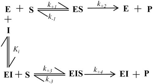
Without pretending to present any news on the steady state analysis of an enzymatic reaction, but only aiming to find a rationale for the observed data and to better define the question of the apparent character of the kinetic constants, let’s consider an inhibition process as described in Figure 2. In Figure 2(A) the basic general model of inhibition of an enzyme²⁹ is shown. For the sake of simplicity, let’s avoid cooperative phenomena considering a simple (i.e. Michaelian) enzyme working either in a steady state or in equilibrium conditions. In the scheme, the possibility that the ternary complex may evolve into products (i.e. $0{\le k}_{+4}\le k_{+2}$), leading to an incomplete inhibition, is considered.

Figure 2. Inhibition models of an enzyme (E): a general model of inhibition (Panel A) and an alternative model of inhibition following “the classical approach” (Panel B). (S): substrate; (I): inhibitor; (ES): enzyme-substrate complex; (EI): enzyme-inhibitor complex; (EIS): enzyme-inhibitor-substrate ternary complex; k₊₁, k₋₁, k₊₂, k₊₃, k₋₃, k₊₄ refer to kinetic constants; K_i and K’_i refer to EI and EIS dissociation constants, respectively. See text for details.

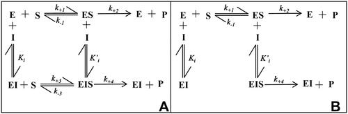
Taking advantage of the microscopic reversibility principle, it is common practice to represent the inhibitory action as in Panel B (the “classical approach”), in which the inhibitor is considered to target either the free enzyme or/and the ES complex. Then, the inhibitor will be defined, due to the relative values of apparent inhibition constants, as “competitive”, “mixed non-competitive” or “uncompetitive”³⁰.

Let’s consider for the moment the very frequent condition of a complete inhibition (i.e. k₊₄ = 0). In this case, ^appV_max ranges from k₊₂[E_T] to zero with the increase of the inhibitor concentration, depending on the factor (1 + [I]$/{K^{\mathrm{\prime }}}_i$)⁻¹; at the same time, ^appK_M may either increase, when $K_i{{<K}^{\mathrm{\prime }}}_i,$ or decrease, when $K_i{{>K}^{\mathrm{\prime }}}_i,$ to a maximum of $K_M\left(1+\left[I\right]/K_i\right)$ or to a minimum of $K_M/\left(1+\left[I\right]/{K^{\mathrm{\prime }}}_i\right),$ respectively. $${}^{\mathit{app}}{K}_M=K_M\frac{\left(1+\frac{\left[I\right]}{K_i}\right)}{\left(1+\frac{\left[I\right]}{K_i^{\mathrm{\prime }}}\right)}$$

Now, looking at the relative changes between the ^appK_M and ^appV_max, going from a mixed inhibition model to an uncompetitive model, the slope of ^appK_M/^appV_max = f ([I]), will decrease from positive values to zero. Such a limit, which refers to the uncompetitive model of inhibition, is the result of the fact that both K_M and V_max decrease of the same factor $\left(1+\left[I\right]/{K^{\mathrm{\prime }}}_i\right).$

It is evident that this approach fails in giving a rationale for the inhibition data reported above (Figure 1), in which ^appK_M/^appV_max versus [I] decreases. ^appK_M can either increase or decrease with, at maximum, the same steepness of ^appV_max. If we (at the moment) rule out that the inhibitor may induce an increase in the affinity of the enzyme for the substrate, the explanation of a negative slope of the ^appK_M/^appV_max = f ([I]) must be searched in the conversion of the enzyme-substrate complex to products. In other words, the decrease in ^appV_max by increasing [I] must be less steep than the ^appK_M decrease. This situation may occur if the ternary complex is able to evolve to products, as it occurs for incomplete inhibitors. Here the decrease of ^appV_max from k₊₂ [^maxES]= k₊₂ [E_T]) in the absence of the inhibitor, will not tend to zero, with the increase of [I] but to ^appV_max =k₊₄ [^maxESI]= k₊₄ [E_T] (See Figure 2(B)).

For the sake of simplicity, let’s consider an incomplete uncompetitive inhibition (K_i at least 100 times higher than K_i’) in which ^appK_M can only decrease when the inhibitor is present. In this case (see Appendix I), considering the assumption of conversion of EIS to product, the model must be analysed in steady state conditions in order to avoid losing the kinetic effect on the ^appK_M changes. Then, the analytic approach in steady state conditions for both ES and EIS, will lead to the following rate equation: (1) $$\frac{v_0}{E_T}=\frac{\frac{{K_i^{\mathrm{*}}k}_{+2}+k_{+4}\left[I\right]}{K_i^{\mathrm{*}}+\left[I\right]}\left[S\right]}{\frac{K_i^{\mathrm{*}}{K}_M+\frac{k_{+4}\left[I\right]}{k_{+1}}}{K_i^{\mathrm{*}}+\left[I\right]}+\left[S\right]}$$(1)

The apparent kinetic constants ${}^{\mathit{app}}{k}_{\mathit{cat}},$ ${}^{\mathit{app}}{K}_M\mathrm{ }$ and ^appK_M/^appk_cat are defined as follows: (2) $${}^{\mathit{app}}{k}_{\mathit{cat}}=\frac{{K_i^{\mathrm{*}}k}_{+2}+k_{+4}\left[I\right]}{K_i^{\mathrm{*}}+\left[I\right]}\mathrm{ }$$(2) (3) $${}^{\mathit{app}}{K}_M=\frac{K_i^{\mathrm{*}}{K}_M+\frac{k_{+4}}{k_{+1}}\left[I\right]}{K_i^{\mathrm{*}}+\left[I\right]}$$(3) (4) $$\frac{{}^{\mathit{app}}{K}_M}{{}^{\mathit{app}}{k}_{\mathit{cat}}}=\frac{K_i^{\mathrm{*}}{K}_M+\frac{k_{+4}}{k_{+1}}\left[I\right]}{{K_i^{\mathrm{*}}k}_{+2}+k_{+4}\left[I\right]}$$(4)

In these equations$K_i^{\mathrm{*}}=\mathrm{ }\frac{k_{-3}+k_{+4}}{k_{+3}}$ Equation (1)(1) $$\frac{v_0}{E_T}=\frac{\frac{{K_i^{\mathrm{*}}k}_{+2}+k_{+4}\left[I\right]}{K_i^{\mathrm{*}}+\left[I\right]}\left[S\right]}{\frac{K_i^{\mathrm{*}}{K}_M+\frac{k_{+4}\left[I\right]}{k_{+1}}}{K_i^{\mathrm{*}}+\left[I\right]}+\left[S\right]}$$(1) defines a hyperbola as a function of substrate concentration, as it occurs for k₊₄ = 0. The dependence of the kinetic parameters ${}^{\mathit{app}}{k}_{\mathit{cat}}$ and ${}^{\mathit{app}}{K}_M$ (Equations 2(2) $${}^{\mathit{app}}{k}_{\mathit{cat}}=\frac{{K_i^{\mathrm{*}}k}_{+2}+k_{+4}\left[I\right]}{K_i^{\mathrm{*}}+\left[I\right]}\mathrm{ }$$(2) and 3(3) $${}^{\mathit{app}}{K}_M=\frac{K_i^{\mathrm{*}}{K}_M+\frac{k_{+4}}{k_{+1}}\left[I\right]}{K_i^{\mathrm{*}}+\left[I\right]}$$(3) ), upon the inhibitor, concentration is expected to have an exponential behaviour approaching an asymptote value >0 (Figure 3). In this regard, it is worth noting that the inclusion of the $k_{+4}$ term (>0) in the $K_i^{\mathrm{*}}$ implies an effect of the incomplete inhibition not only, as expected, on ^appV_max, but also on ${}^{\mathit{app}}{K}_M.$ In fact, instead of tending to zero, when the inhibitor concentration increases, ${}^{\mathit{app}}{K}_M$ will asymptotically tend to $\frac{k_{+4}}{k_{+1}}.$ Thus, it appears from this analysis that the decrease of both ^appV_max and ^appK_M is buffered when EIS is able to evolve to products. Nevertheless, ^appK_M will tend to a value ($\frac{k_{+4}}{k_{+1}}$) reasonably much lower than k₊₄, which is the limit value for ^appV_max, thus giving the rationale for the decrease of ^appK_M/^appk_cat versus [I] (Equation (4)(4) $$\frac{{}^{\mathit{app}}{K}_M}{{}^{\mathit{app}}{k}_{\mathit{cat}}}=\frac{K_i^{\mathrm{*}}{K}_M+\frac{k_{+4}}{k_{+1}}\left[I\right]}{{K_i^{\mathrm{*}}k}_{+2}+k_{+4}\left[I\right]}$$(4) , Figure 3(C)).

Figure 3. Incomplete uncompetitive inhibition. (Panel A) represents the dependence of ^appk_cat on the increase of [I] according to Equation (2)(2) $${}^{\mathit{app}}{k}_{\mathit{cat}}=\frac{{K_i^{\mathrm{*}}k}_{+2}+k_{+4}\left[I\right]}{K_i^{\mathrm{*}}+\left[I\right]}\mathrm{ }$$(2) ; (Panel B) represents the dependence of ^appk_M on the increase of [I] according to Equation (3)(3) $${}^{\mathit{app}}{K}_M=\frac{K_i^{\mathrm{*}}{K}_M+\frac{k_{+4}}{k_{+1}}\left[I\right]}{K_i^{\mathrm{*}}+\left[I\right]}$$(3) ; (Panel C) represents the dependence of ^appK_M/^appk_cat on the increase of [I] according to Equation (4)(4) $$\frac{{}^{\mathit{app}}{K}_M}{{}^{\mathit{app}}{k}_{\mathit{cat}}}=\frac{K_i^{\mathrm{*}}{K}_M+\frac{k_{+4}}{k_{+1}}\left[I\right]}{{K_i^{\mathrm{*}}k}_{+2}+k_{+4}\left[I\right]}$$(4) .

Independently on the inhibition model, the evaluation of the incomplete action of an inhibitor is not an easy task, especially when k₊₄ is rather low. Indeed, looking at the significant effect on the ^appK_M/^appk_cat versus [I] exerted by relative small values of k₊₄ with respect to k₊₂ (Figure 4), it appears that the experimental observation of a decrease of ^appK_M/^appk_cat versus the inhibitor concentration becomes a valuable indication that the inhibition is not complete.

Figure 4. Predicted effect of the inhibitor concentration on the apparent kinetic parameters. The dependence of 1/^appk_cat (Panel A) and ^appK_M/^appk_cat (Panel B) on the inhibitor concentration for different incomplete uncompetitive inhibition situations is reported, according to Equations (2(2) $${}^{\mathit{app}}{k}_{\mathit{cat}}=\frac{{K_i^{\mathrm{*}}k}_{+2}+k_{+4}\left[I\right]}{K_i^{\mathrm{*}}+\left[I\right]}\mathrm{ }$$(2) and 4)(4) $$\frac{{}^{\mathit{app}}{K}_M}{{}^{\mathit{app}}{k}_{\mathit{cat}}}=\frac{K_i^{\mathrm{*}}{K}_M+\frac{k_{+4}}{k_{+1}}\left[I\right]}{{K_i^{\mathrm{*}}k}_{+2}+k_{+4}\left[I\right]}$$(4) , respectively. The following arbitrary values were fixed: k₊₂ = 1, k₊₁ = 100, K_M = 0.5 and $K_i^{\mathrm{*}}$ = 0.001. Curves 1–6 refer to k₊₄ values of zero (complete inhibition), 0.02, 0.05, 0.1, 0.15 and 0.2, respectively.

This approach will also apply to a mixed inhibition model in which the ^appK_M changes may occur in both directions, depending on the relative apparent values of $K_i^{}$ and $K_i^{\mathrm{\prime }}.\mathrm{ }$ In this case, however, it is obvious that the incomplete inhibitory action of the inhibitor cannot be any more univocally associated with a decrease of the ^appK_M/^appk_cat versus [I].

The rather complex kinetic equation (Equation (5)(5) $$\frac{v_0}{E_T}=\frac{\frac{{K_i^{\mathrm{*}}k}_{+2}+k_{+4}\left[I\right]}{K_i^{\mathrm{*}}+\left[I\right]}\left[S\right]}{\frac{K_M{K}_i^{\mathrm{*}}+\left(\frac{K_i^{\mathrm{*}}}{K_i}{K}_M+\frac{k_{+4}}{k_{+1}}\right)\left[I\right]+\frac{k_{+4}}{{K_{i}k}_{+1}}{\left[I\right]}^2}{K_i^{\mathrm{*}}+\left[I\right]}+\left[S\right]}$$(5) for a mixed inhibition model, derived from a steady state assumption for ES and EIS and an equilibrium assumption for EI (see Appendix II) still defines a hyperbola as a function of substrate concentration. (5) $$\frac{v_0}{E_T}=\frac{\frac{{K_i^{\mathrm{*}}k}_{+2}+k_{+4}\left[I\right]}{K_i^{\mathrm{*}}+\left[I\right]}\left[S\right]}{\frac{K_M{K}_i^{\mathrm{*}}+\left(\frac{K_i^{\mathrm{*}}}{K_i}{K}_M+\frac{k_{+4}}{k_{+1}}\right)\left[I\right]+\frac{k_{+4}}{{K_{i}k}_{+1}}{\left[I\right]}^2}{K_i^{\mathrm{*}}+\left[I\right]}+\left[S\right]}$$(5)

The apparent kinetic constants ${}^{\mathit{app}}{k}_{\mathit{cat}},$ ${}^{\mathit{app}}{K}_M\mathrm{ }$ and ^appK_M/^appk_cat are defined as follows: (6) $${}^{\mathit{app}}{k}_{\mathit{cat}}=\frac{{K_i^{\mathrm{*}}k}_{+2}+k_{+4}\left[I\right]}{K_i^{\mathrm{*}}+\left[I\right]}\mathrm{ }$$(6) (7) $${}^{\mathit{app}}{K}_M=\frac{K_M{K}_i^{\mathrm{*}}+\left(\frac{K_i^{\mathrm{*}}}{K_i}{K}_M+\frac{k_{+4}}{k_{+1}}\right)\left[I\right]+\frac{k_{+4}}{{K_{i}k}_{+1}}{\left[I\right]}^2}{K_i^{\mathrm{*}}+\left[I\right]}\mathrm{ }$$(7) (8) $$\frac{{{}^{\mathit{app}}K}_M^{}}{{{}^{\mathit{app}}k}_{\mathit{cat}}^{}}=\frac{\mathrm{ }{K}_M{K}_i^{\mathrm{*}}+\left(\frac{K_i^{\mathrm{*}}}{K_i}{K}_M+\frac{k_{+4}}{k_{+1}}\right)\left[I\right]+\frac{k_{+4}}{{K_{i}k}_{+1}}{\left[I\right]}^2}{{K_i^{\mathrm{*}}k}_{+2}+k_{+4}\left[I\right]}$$(8)

Figure 5 reports the predicted effect of inhibitor concentration on apparent kinetic parameters.

Figure 5. Predicted effect of the inhibitor concentration on the apparent kinetic parameters. The dependence of 1/^appk_cat (Panels A and D), ^appK_M (Panels B and E) and ^appK_M/^appk_cat (Panels C and F) on the inhibitor concentration for different incomplete mixed inhibition situations is reported, according to Equations (6–8), respectively. The following arbitrary values were fixed: k₊₂ = 1, k₊₁ = 100, K_M = 0.5. Curves 1–6 refer to k₊₄ values of zero (complete inhibition), 0.02, 0.05, 0.1, 0.15 and 0.2, respectively. (Panels A–C) refer to $K_i^{\mathrm{*}}$ and K_i values of 0.001 and 0.01, respectively. (Panels D–F) refer to $K_i^{\mathrm{*}}$ and K_i values of 0.01 and 0.001 respectively. In (Panels B and E), curves 1–6 are essentially superimposable. Having imposed a reasonable rather low value of k₊₂/k₊₁ (0.01), k₊₄/k₊₁ will be negligible making the curves of ^appK_M versus [I] at different k₊₄ are essentially superimposable.

It is clearly evident in Figure 5 the effect of the $K_i^{\mathrm{*}}$/$K_i^{}$ the ratio on the dependence of ^appK_M and of ^appK_M/^appk_cat on inhibitor concentration. Thus, while a decrease of ^appK_M/^appk_cat versus [I] is a univocal indication of an incomplete inhibition phenomenon, the incomplete inhibition cannot be ruled out when an increase of ^appK_M/^appk_cat versus [I] is observed.

To conclude, once verified the occurrence of an incomplete inhibition, the above classical approach may give the rationale even for the experimental observation of a decrease of ^appK_M/^appk_cat versus [I] as reported for EGCG in Figure 1. However, as shown, when the inhibition is not complete (i.e. 0<k₊₄<k₊₂), we must expect an exponential trend (either an increase or a decrease) of 1/^appk_cat, 1/^appK_M or ^appK_M/^appk_cat as a function of [I]. Thus, the possible apparent linearity of experimental plots (i.e. 1/^appk_cat, 1/^appK_M or ^appK_M/^appk_cat versus [I]) may be part of an overall exponential function. In any case, the analysis of experimental data must be performed through nonlinear regression.

Kinetic models of enzyme inhibition: the non-classical approach

As mentioned in the introduction, serious problems may be encountered in attempting to correlate the apparent inhibitory constants, with a physical interactive model. In fact, a different legitimate model of action, absolutely equivalent to the classic approach, is the one reported in Figure 6, in which the equilibrium generating ESI is omitted, based on the microscopic reversibility principle.

Figure 6. Inhibition model of an enzyme (E) following “the non-classical approach”. (S): substrate; (I): inhibitor; (ES): enzyme-substrate complex; (EI): enzyme-inhibitor complex; (EIS): ternary enzyme-inhibitor-substrate complex; k₊₁, k₋₁, k₊₂, k₊₃, k₋₃, k₊₄ are kinetic constants; K_i is the EI complex dissociation constant. See text for details.

Here, the interaction of the inhibitor with the enzyme is described through a unique event, and it is the substrate that interacts either with the free enzyme or with the inhibitor-enzyme (EI) complex. It is evident that the interpretation of the same experimental data v₀ = f ([S], [I]) will lead, now, to a completely different conclusion with respect to the classical approach.

The apparently simplest non-classical model is the case of a complete inhibition, which refers to the scheme of Figure 6 in which k₊₄ = 0. In this case (see Appendix III), from a steady state condition for ES and an equilibrium condition for both EI and EIS, the following kinetic equation will be obtained: (9) $$\frac{v_0}{E_T}=\frac{\frac{k_{+2}}{1+\frac{\left[I\right]K_M}{K_M^{\mathrm{\prime }}{K}_i}}\left[S\right]}{\frac{K_M\left(1+\frac{\left[I\right]}{K_i}\right)}{1+\frac{\left[I\right]K_M}{K_M^{\mathrm{\prime }}{K}_i}}+\left[S\right]\mathrm{ }}$$(9)

In Equation (9)(9) $$\frac{v_0}{E_T}=\frac{\frac{k_{+2}}{1+\frac{\left[I\right]K_M}{K_M^{\mathrm{\prime }}{K}_i}}\left[S\right]}{\frac{K_M\left(1+\frac{\left[I\right]}{K_i}\right)}{1+\frac{\left[I\right]K_M}{K_M^{\mathrm{\prime }}{K}_i}}+\left[S\right]\mathrm{ }}$$(9) , $K_M^{\mathrm{\prime }}$ represents the dissociation constant for the ternary complex EIS, $\left({\mathrm{i}.\mathrm{e}.\mathrm{ }K}_M^{\mathrm{\prime }}=k_{-3}/k_{+3}\right).$

The apparent kinetic constants are defined as follows: (10) $${}^{\mathit{app}}{K}_M=\frac{k_M\left(1+\frac{\left[I\right]}{K_i}\right)}{1+\frac{\left[I\right]k_M}{K_i{K}_M^{\mathrm{\prime }}}}\mathrm{ }$$(10) (11) $${}^{\mathit{app}}{k}_{\mathit{cat}}=\frac{{K_i{K}_M^{\mathrm{\prime }}k}_{+2}}{K_i{K}_M^{\mathrm{\prime }}+k_M\left[I\right]}$$(11) (12) $$\frac{{}^{\mathit{app}}{K}_M}{{}^{\mathit{app}}{k}_{\mathit{cat}}}=\frac{K_M}{k_{+2}}+\frac{K_M}{K_i{k}_{+2}}\left[I\right]\mathrm{ }$$(12)

The dependence of the kinetic parameters (Equations 10–12), upon the inhibitor concentration, is reported in Figure 7; here is supposed that K’_M>K_M. It is evident that a different affinity of the substrate for E and EI will not affect the progressive decline of ^appk_cat to zero, so that ${}^{\mathit{app}}{K}_M/{}^{\mathit{app}}{k}_{\mathrm{cat}}$ will increase with the increase of [I] (Figure 7(B, C)).

Figure 7. Non-classical approach for complete inhibition. (Panel A) represents the dependence of ^appK_M on the increase of [I] according to Equation (10)(10) $${}^{\mathit{app}}{K}_M=\frac{k_M\left(1+\frac{\left[I\right]}{K_i}\right)}{1+\frac{\left[I\right]k_M}{K_i{K}_M^{\mathrm{\prime }}}}\mathrm{ }$$(10) ; (Panel B) represents the dependence of 1/^appk_cat on the increase of [I] according to Equation (11)(11) $${}^{\mathit{app}}{k}_{\mathit{cat}}=\frac{{K_i{K}_M^{\mathrm{\prime }}k}_{+2}}{K_i{K}_M^{\mathrm{\prime }}+k_M\left[I\right]}$$(11) ; Panel C represents the dependence of ^appK_M/^appk_cat on the increase of [I] according to Equation (12)(12) $$\frac{{}^{\mathit{app}}{K}_M}{{}^{\mathit{app}}{k}_{\mathit{cat}}}=\frac{K_M}{k_{+2}}+\frac{K_M}{K_i{k}_{+2}}\left[I\right]\mathrm{ }$$(12) .

When an incomplete inhibition for the non-classical inhibition model is considered (i.e. 0<k₊₄ <k₊₂) (Figure 6), the analysis performed considering the steady state for both branches of product formation and the inhibitor binding at equilibrium, leads to the following kinetic equation (see Appendix IV). (13) $$\frac{v_0}{E_T}=\frac{\frac{k_{+2}{K}_M^{\mathrm{\prime }}{K}_i+k_{+4}{K}_M\left[I\right]}{K_M\left[I\right]+K_M^{\mathrm{\prime }}{K}_i}\left[S\right]}{\frac{K_M{K}_M^{\mathrm{\prime }}\left(K_i+\left[I\right]\right)}{K_M^{\mathrm{\prime }}{K}_i+K_M\left[I\right]}+\left[S\right]}$$(13) in which $K_M=\frac{k_{-1}+k_{+2}}{k_{+1}},$ ${K\mathrm{ }}_M^{\mathrm{\prime }}=\frac{k_{-3}+k_{+4}}{k_{+3}}$ and $K_i=\frac{\left[E\right]\left[I\right]}{\left[EI\right]}$

The apparent kinetic parameters are defined as follows: (14) $${}^{\mathit{app}}{K}_M=\frac{{K_{i}K}_M{K}_M^{\mathrm{\prime }}+K_M{K}_M^{\mathrm{\prime }}\left[I\right]}{{K_M^{\mathrm{\prime }}{K}_i+K}_M\left[I\right]}$$(14) (15) $${{}^{\mathit{app}}k}_{\mathit{cat}}=\mathrm{ }\frac{k_{+2}{K}_M^{\mathrm{\prime }}{K}_i+k_{+4}{K}_M\left[I\right]}{K_M^{\mathrm{\prime }}{K}_i{+\mathrm{ }K}_M\left[I\right]}$$(15) (16) $$\frac{{}^{\mathit{app}}{K}_M}{{{}^{\mathit{app}}k}_{\mathit{cat}}}=\frac{{K_{i}K}_M{K}_M^{\mathrm{\prime }}+K_M{K}_M^{\mathrm{\prime }}\left[I\right]}{k_{+2}{K}_M^{\mathrm{\prime }}{K}_i+k_{+4}{K}_M\left[I\right]}$$(16)

The dependence of the kinetic parameters (Equations (14)–(16)), upon the inhibitor concentration, is reported in Figure 8. Also in this case K’_M>K_M is assumed.

Figure 8. Non-classical approach for incomplete inhibition. (Panel A) represents the dependence of ^appK_M on the increase of [I] according to Equation (14)(14) $${}^{\mathit{app}}{K}_M=\frac{{K_{i}K}_M{K}_M^{\mathrm{\prime }}+K_M{K}_M^{\mathrm{\prime }}\left[I\right]}{{K_M^{\mathrm{\prime }}{K}_i+K}_M\left[I\right]}$$(14) ; (Panel B) represents the dependence of 1/^appk_cat on the increase of [I] according to Equation (15)(15) $${{}^{\mathit{app}}k}_{\mathit{cat}}=\mathrm{ }\frac{k_{+2}{K}_M^{\mathrm{\prime }}{K}_i+k_{+4}{K}_M\left[I\right]}{K_M^{\mathrm{\prime }}{K}_i{+\mathrm{ }K}_M\left[I\right]}$$(15) ; (Panel C) represents the dependence of ^appK_M/^appk_cat on the increase of [I] according to Equation (16)(16) $$\frac{{}^{\mathit{app}}{K}_M}{{{}^{\mathit{app}}k}_{\mathit{cat}}}=\frac{{K_{i}K}_M{K}_M^{\mathrm{\prime }}+K_M{K}_M^{\mathrm{\prime }}\left[I\right]}{k_{+2}{K}_M^{\mathrm{\prime }}{K}_i+k_{+4}{K}_M\left[I\right]}$$(16) .

This approach predicts that the substrate binds to EI, leading to a ternary complex that is susceptible to transformation to products. Here, except for the parameters related to the not inhibited reaction (i.e. [I] = 0), and for the definition of the kinetic parameter k₊₄, which defines the ability of EIS to generate products, the meaning of axis intercepts and asymptotic values of the graphs is completely different from those emerging from the classical approach. It is worth noting that, for the non-classic kinetic model, the limit values of ^appK_M (i.e. K_M and K’_M) represent intrinsic features of the substrate when interacting with two different enzyme forms (i.e. E and EI), whose relative abundance is the consequence only of the efficiency of the inhibitor in binding the free enzyme.

Having imposed k₊₄<k₊₂ and K’_M>K_M it will be difficult to envisage a decrease of ^appK_M/^appk_cat versus [I]. However, a decrease may occur either when k₊₄/k₊₂ > K’_M/K_M or, more intriguingly, admitting a positive effect of the inhibitor on the binding of the substrate (i.e. K’_M < K_M).

Kinetic analysis of AKR1B1 inhibition by EGCG

The above considerations offer a rationale for a more adequate fitting of the results shown in Figure 1, obtained when EGCG was tested as an inhibitor of the AKR1B1-dependent reduction of HNE. Here, the original experimental points are reported in Figure 9(A). The resulting ^appK_M and ^appk_cat values, obtained at different EGCG concentrations, were analysed through nonlinear regression using Equations (6(6) $${}^{\mathit{app}}{k}_{\mathit{cat}}=\frac{{K_i^{\mathrm{*}}k}_{+2}+k_{+4}\left[I\right]}{K_i^{\mathrm{*}}+\left[I\right]}\mathrm{ }$$(6) and 7)(7) $${}^{\mathit{app}}{K}_M=\frac{K_M{K}_i^{\mathrm{*}}+\left(\frac{K_i^{\mathrm{*}}}{K_i}{K}_M+\frac{k_{+4}}{k_{+1}}\right)\left[I\right]+\frac{k_{+4}}{{K_{i}k}_{+1}}{\left[I\right]}^2}{K_i^{\mathrm{*}}+\left[I\right]}\mathrm{ }$$(7) , respectively (Figure 9(B, C)). To evaluate the apparent dissociation constant of EIS (K_i*) and the kinetic constant of the ternary complex (k₊₄), a k_cat value of 78 min⁻¹ (78 ± 4 min⁻¹) for HNE reduction in the absence of the inhibitor was inserted in Equation (6)(6) $${}^{\mathit{app}}{k}_{\mathit{cat}}=\frac{{K_i^{\mathrm{*}}k}_{+2}+k_{+4}\left[I\right]}{K_i^{\mathrm{*}}+\left[I\right]}\mathrm{ }$$(6) , as k₊₂. To determine the ES dissociation constant (K_i), whose value was imposed being >0, a value of 51 µM (51 ± 5 µM) for the K_M for the substrate HNE in the absence of EGCG was used. Once verified the expected extremely low values of k₊₄/k_‒1, Equations (7(7) $${}^{\mathit{app}}{K}_M=\frac{K_M{K}_i^{\mathrm{*}}+\left(\frac{K_i^{\mathrm{*}}}{K_i}{K}_M+\frac{k_{+4}}{k_{+1}}\right)\left[I\right]+\frac{k_{+4}}{{K_{i}k}_{+1}}{\left[I\right]}^2}{K_i^{\mathrm{*}}+\left[I\right]}\mathrm{ }$$(7) and 8)(8) $$\frac{{{}^{\mathit{app}}K}_M^{}}{{{}^{\mathit{app}}k}_{\mathit{cat}}^{}}=\frac{\mathrm{ }{K}_M{K}_i^{\mathrm{*}}+\left(\frac{K_i^{\mathrm{*}}}{K_i}{K}_M+\frac{k_{+4}}{k_{+1}}\right)\left[I\right]+\frac{k_{+4}}{{K_{i}k}_{+1}}{\left[I\right]}^2}{{K_i^{\mathrm{*}}k}_{+2}+k_{+4}\left[I\right]}$$(8) could be simplified assuming this ratio equals to zero. Finally, since K_i value resulted far exceeding the K_i* value of 124 ± 19 µM (K_i/K_i*>100), the ^appK_M/^appk_cat versus [I] data were interpolated by Equation (4)(4) $$\frac{{}^{\mathit{app}}{K}_M}{{}^{\mathit{app}}{k}_{\mathit{cat}}}=\frac{K_i^{\mathrm{*}}{K}_M+\frac{k_{+4}}{k_{+1}}\left[I\right]}{{K_i^{\mathrm{*}}k}_{+2}+k_{+4}\left[I\right]}$$(4) as an uncompetitive inhibition. The insertion of the above K_i* value in Equation (4)(4) $$\frac{{}^{\mathit{app}}{K}_M}{{}^{\mathit{app}}{k}_{\mathit{cat}}}=\frac{K_i^{\mathrm{*}}{K}_M+\frac{k_{+4}}{k_{+1}}\left[I\right]}{{K_i^{\mathrm{*}}k}_{+2}+k_{+4}\left[I\right]}$$(4) , in which no restrictions were imposed to k₊₄, gives rise to the curve fitting of the experimental data shown in Figure 9(D), to be compared with that used in Figure 1. The curve fitting allowed to obtain a k₊₄ value of 17 ± 2 min⁻¹. In conclusion, these data, besides confirming the uncompetitive action of EGCG on the AKR1B1-dependent HNE reduction (K_i’ = 116 ± 11 μM)⁵, disclose the occurrence of an incomplete inhibition. This phenomenon is characterised by a k₊₄ of 12 ± 2 min⁻¹, as the average of values emerging from ^appK_M/^appk_cat versus [I] (Equation (4)(4) $$\frac{{}^{\mathit{app}}{K}_M}{{}^{\mathit{app}}{k}_{\mathit{cat}}}=\frac{K_i^{\mathrm{*}}{K}_M+\frac{k_{+4}}{k_{+1}}\left[I\right]}{{K_i^{\mathrm{*}}k}_{+2}+k_{+4}\left[I\right]}$$(4) ) and 1/^appk_cat versus [I] (Equation (2)(2) $${}^{\mathit{app}}{k}_{\mathit{cat}}=\frac{{K_i^{\mathrm{*}}k}_{+2}+k_{+4}\left[I\right]}{K_i^{\mathrm{*}}+\left[I\right]}\mathrm{ }$$(2) ) plots. Thus, the inhibition of EGCG leads to residual activity of approximately 15% of the reaction rate measured in the absence of the inhibitor.

Figure 9. Kinetic analysis by the classical approach of EGCG inhibition of the AKR1B1-dependent reduction of HNE. (Panel A) Hanes-Wolff representation of rate measurements of HNE reduction in the presence of the indicated concentrations of EGCG. Bars (when not visible are within the symbols size) represent the standard deviations of the means from at least three independent measurements. (Panels B–D) secondary plots of apparent kinetic parameters at different [I] derived from the non-linear regression Michaelis-Menten analysis of primary kinetic data. Bars (when not visible are within the symbols size) represent the standard error of the measurements. The parameters ^appK_M, 1/^appk_cat and ^appK_M/^appk_cat versus [I] were interpolated by non-linear regression analysis according to Equations (4)(6) $${}^{\mathit{app}}{k}_{\mathit{cat}}=\frac{{K_i^{\mathrm{*}}k}_{+2}+k_{+4}\left[I\right]}{K_i^{\mathrm{*}}+\left[I\right]}\mathrm{ }$$(6) , (6)(7) $${}^{\mathit{app}}{K}_M=\frac{K_M{K}_i^{\mathrm{*}}+\left(\frac{K_i^{\mathrm{*}}}{K_i}{K}_M+\frac{k_{+4}}{k_{+1}}\right)\left[I\right]+\frac{k_{+4}}{{K_{i}k}_{+1}}{\left[I\right]}^2}{K_i^{\mathrm{*}}+\left[I\right]}\mathrm{ }$$(7) and (7)(4) $$\frac{{}^{\mathit{app}}{K}_M}{{}^{\mathit{app}}{k}_{\mathit{cat}}}=\frac{K_i^{\mathrm{*}}{K}_M+\frac{k_{+4}}{k_{+1}}\left[I\right]}{{K_i^{\mathrm{*}}k}_{+2}+k_{+4}\left[I\right]}$$(4) , respectively. See the text for details.

This analysis was applied also to the inhibition by EGCG on L-idose reduction, considering a k₊₂ of 195 min⁻¹ (195 ± 6 min⁻¹) and a $K_M$ of 4.26 mM (4.26 ± 0.35 mM) measured in the absence of the inhibitor. In this case (Figure 10), a classical behaviour as a mixed type of complete inhibition was verified, with a k₊₄ of 1.7 ± 0.5 min⁻¹ (i.e. less than 1% of k₊₂) and K_i* and K_i values of 75 ± 2 µM and 330 ± 26 µM, respectively. These values were in line with previous characterisation (61 ± 9 µM and 425 ± 64 µM for K_i’ and K_i, respectively)⁵.

Figure 10. Kinetic analysis by the classical approach of EGCG inhibition of the AKR1B1-dependent reduction of L-idose. (Panel A) Hanes-Wolff representation of rate measurements of L-idose reduction in the presence of the indicated concentrations of EGCG. Bars (when not visible are within the symbols size) represent the standard deviations of the means from at least three independent measurements. (Panels B–D) secondary plots of apparent kinetic parameters at different [I] coming from the non-linear regression Michaelis-Menten analysis of primary kinetic data. Bars (when not visible are within the symbols size) represent the standard error of the measurements. The parameters ^appK_M, ^appk_cat and ^appK_M/^appk_cat versus [I] were interpolated by non-linear regression analysis through Equations (4)(6) $${}^{\mathit{app}}{k}_{\mathit{cat}}=\frac{{K_i^{\mathrm{*}}k}_{+2}+k_{+4}\left[I\right]}{K_i^{\mathrm{*}}+\left[I\right]}\mathrm{ }$$(6) , (6) and (7), respectively.

In light of the above mechanistic considerations, while the inhibition by EGCG on L-idose reduction is confirmed to fit a classical mixed type of complete inhibition, a rationale for the data observed for the same inhibitor on HNE reduction can be envisaged. In fact, the decrease of ^appK_M/^appk_cat versus [I] appears as the result of the combined effect of an incomplete and uncompetitive inhibition. As predicted by the above kinetic models, in fact, both conditions are required to observe the phenomenon. It emerges from the study that a negative trend of ^appK_M/^appk_cat with the increase of the inhibitor, concentration is an indication that an incomplete inhibition is occurring. This may be useful, especially when the residual activity upon inhibition is rather low. In these cases, the identification of the incompleteness of the inhibitory process may not result in an easy task due to the low reliability of rate measurements at high inhibitor concentrations.

Concerning the non-classical model analysis (Figure 6) of the above inhibitory data, rate measurements in the presence of HNE (Figure 9(A)) or L-idose (Figure 10(A)) at different inhibitor concentrations were analysed through regression analysis of Equations (9)(9) $$\frac{v_0}{E_T}=\frac{\frac{k_{+2}}{1+\frac{\left[I\right]K_M}{K_M^{\mathrm{\prime }}{K}_i}}\left[S\right]}{\frac{K_M\left(1+\frac{\left[I\right]}{K_i}\right)}{1+\frac{\left[I\right]K_M}{K_M^{\mathrm{\prime }}{K}_i}}+\left[S\right]\mathrm{ }}$$(9) and (13)(13) $$\frac{v_0}{E_T}=\frac{\frac{k_{+2}{K}_M^{\mathrm{\prime }}{K}_i+k_{+4}{K}_M\left[I\right]}{K_M\left[I\right]+K_M^{\mathrm{\prime }}{K}_i}\left[S\right]}{\frac{K_M{K}_M^{\mathrm{\prime }}\left(K_i+\left[I\right]\right)}{K_M^{\mathrm{\prime }}{K}_i+K_M\left[I\right]}+\left[S\right]}$$(13) , respectively. Being the inhibition of L-idose reduction an apparently complete phenomenon, the emerging values of 1/^appk_cat, ^appK_M and ^appK_M/^appk_cat at different [I], were interpolated through Equations (10)–(12), respectively. The best fitting of the data through the above equations (Figure 11(A–C)) is compatible with an inhibition constant K_i of 385 ± 18 µM and a K’_M of 831 ± 12 µM, accounting for an apparent increase of affinity of the substrate for the EI complex of approximately 5 folds.

Figure 11. Kinetic analysis by the non-classical approach of EGCG inhibition of the AKR1B1-dependent reduction of L-idose. The parameters 1/^appk_cat, ^appK_M and ^appK_M/^appk_cat obtained from data in Figure 10(A), were reported as a function of [I] and interpolated by non-linear regression analysis through Equations (10)–(12), respectively. Bars (when not visible are within the symbols size) represent the standard error of the measurements.

In the case of HNE reduction, for which an incomplete inhibition apparently occurs, a k₊₄ value of 12 ± 4 min⁻¹, as derived from the classic analysis, was used. Here, 1/^appk_cat, ^appK_M and ^appK_M/^appk_cat were derived from Equation (13)(13) $$\frac{v_0}{E_T}=\frac{\frac{k_{+2}{K}_M^{\mathrm{\prime }}{K}_i+k_{+4}{K}_M\left[I\right]}{K_M\left[I\right]+K_M^{\mathrm{\prime }}{K}_i}\left[S\right]}{\frac{K_M{K}_M^{\mathrm{\prime }}\left(K_i+\left[I\right]\right)}{K_M^{\mathrm{\prime }}{K}_i+K_M\left[I\right]}+\left[S\right]}$$(13) at different [I]. The secondary plots of the obtained data as a function of [I], (Figure 12(A–C)) were interpolated through Equations (14)–(16), respectively.

Figure 12. Kinetic analysis by the non-classical approach of EGCG inhibition of the AKR1B1-dependent reduction of HNE. The parameters 1/^appk_cat, ^appK_M and ^appK_M/^appk_cat obtained from data in Figure 9(A), were reported as a function of [I] and interpolated by non-linear regression analysis through Equations (14)–(16), respectively. Bars (when not visible are within the symbols size) represent the standard error of the measurements.

In this case, an acceptable, even though not optimal, fitting of the data, including the decline of ^appK_M/^appk_cat versus [I] was observed. However, the values of the kinetic parameters emerging from this interpolation were, unfortunately, corrupted by very high uncertainty determination (K_i =4,626 ± 25,000 and K’_M = 0.9 ± 4) to be worthy of further consideration. It is hard to envisage whether such an unsatisfactory result derives from a different possible error propagation in the latter analysis or/and from the strong restrictions required by the model to be applicable. In fact, admitting valid the emerging high K_i value (which, incidentally, is in line with the uncompetitive action resulting from the classical analysis), a marked increase in the affinity of the HNE for the EI complex, with respect to the free enzyme, of approximately 50 folds would be required in order to fit the model. To support this interpretation and to confirm the model, an improvement of kinetic measurements and/or the availability of experimental data from a non-kinetic approach would be necessary.

The possibility to select between the two models, thus going inside the mechanism, necessarily requires the extension of the inhibition study to measurements not related to the steady state kinetic analysis. Thus, for instance, the evaluation of binding constants coming from fast kinetic approaches, spectroscopic and/or calorimetric measurements, or computational analysis might be considered.

In conclusion, the view of a differential inhibition as the result of a different targeting of an inhibitor depending on the substrate undergoing transformation can be changed, through the non-classic model approach, towards a kinetic equivalent view, which implies that different substrates differently target the EI complex. In any case, specifically referring to aldose reductase, the incomplete inhibition discovered for EGCG, which exclusively targets HNE reduction, discloses a new aspect to be furthered in searching for differential inhibitors, molecules that should preferentially inhibit the deleterious glucose reduction while preserving the reduction of toxic aldehydes.

Disclosure statement

The authors report there are no competing interests to declare.

Additional information

Funding

This work was supported by the Pisa University, “Fondi di Ateneo.”

Appendix I

Incomplete uncompetitive inhibition

Referring to Figure 2(B), the analysis is performed by assuming that $${K_{i\mathrm{ }}\gg (K}_i^{\mathrm{\prime }}=\frac{k_{-3}}{k_{+3}})$$ with $k_{+3}$ and $k_{-3}$ as the kinetic constants of EIS formation and dissociation to ES, respectively. The model is analysed by assuming both ES and EIS are in steady state conditions.

It follows a general kinetic equation as: (A.1) $$v_0=\mathrm{ }{k}_{+2}\left[ES\right]+k_{+4}\left[\mathit{EIS}\right]$$(A.1) and an enzyme mass balance equation as: (A.2) $$E_T=\left[E\right]+\left[ES\right]+\left[\mathit{EIS}\right]$$(A.2)

The steady state conditions for both ES and EIS will be: (A.3) $$k_{+1}\left[E\right]\left[S\right]+k_{-3}\left[\mathit{EIS}\right]=\left(k_{+2}+k_{-1}\right)\mathrm{ }\left[ES\right]+k_{+3}\left[I\right]\left[ES\right]$$(A.3) (A.4) $$k_{+3}\left[I\right]\left[ES\right]=\mathrm{ }\left(k_{-3}+k_{+4}\right)\mathrm{ }\left[\mathit{EIS}\right]$$(A.4)

From (A.4): (A.5) $$\left[\mathit{EIS}\right]=\frac{\left[I\right]\left[ES\right]}{K_i^{\mathrm{*}}}$$(A.5) in which $K_i^{\mathrm{*}}=\left(\frac{k_{-3}+k_{+4}}{k_{+3}}\right)$

Replacing $\left[\mathit{EIS}\right]$ in (A.3) and resolving for $\left[E\right]$ (A.6) $$\left[E\right]=\frac{K_i^{\mathrm{*}}\left(k_{+2}+k_{-1}+k_{+3}\left[I\right]\right)-k_{-3}\left[I\right]}{K_i^{\mathrm{*}}{k}_{+1}\left[S\right]}\left[ES\right]$$(A.6)

Replacing $\left[\mathit{EIS}\right]$ and $\left[E\right]\mathrm{ }$(A.5) and (A.6) into the mass balance Equation (A.2)(A.2) $$E_T=\left[E\right]+\left[ES\right]+\left[\mathit{EIS}\right]$$(A.2) : (A.7) $$E_T=\left\{\frac{K_i^{\mathrm{*}}\left(k_{+2}+k_{-1}+k_{+3}\left[I\right]\right)-k_{-3}\left[I\right]+\mathrm{ }{K}_i^{\mathrm{*}}{k}_{+1}\left[S\right]+k_{+1}\left[S\right]\left[I\right]}{K_i^{\mathrm{*}}{k}_{+1}\left[S\right]}\right\}\left[ES\right]$$(A.7)

Replacing$\mathrm{ }\left[\mathit{EIS}\right]$ (A.5) in the rate Equation (A.1)(A.1) $$v_0=\mathrm{ }{k}_{+2}\left[ES\right]+k_{+4}\left[\mathit{EIS}\right]$$(A.1) and then normalising for $E_T$ (A.7) (A.8) $$\frac{v_0}{E_T}=\frac{\left({K_i^{\mathrm{*}}k}_{+2}+k_{+4}\left[I\right]\right)k_{+1}\left[S\right]}{K_i^{\mathrm{*}}\left(k_{+2}+k_{-1}+k_{+3}\left[I\right]\right)-k_{-3}\left[I\right]+\mathrm{ }\left(K_i^{\mathrm{*}}+\left[I\right]\right)k_{+1}\left[S\right]}$$(A.8)

Dividing numerator and denominator by$\left(K_i^{\mathrm{*}}+\left[I\right]\right)k_{+1}$ $$\frac{v_0}{E_T}=\frac{\frac{{K_i^{\mathrm{*}}k}_{+2}+k_{+4}\left[I\right]}{K_i^{\mathrm{*}}+\left[I\right]}\left[S\right]}{\frac{K_i^{\mathrm{*}}\left(k_{+2}+k_{-1}\right)+k_{+4}\left[I\right]}{\left(K_i^{\mathrm{*}}+\left[I\right]\right)k_{+1}}+\mathrm{ }\left[S\right]}$$ and dividing the denominator by $k_{+1}$ the final kinetic equation is obtained: (A.9) $$\frac{v_0}{E_T}=\frac{\frac{{K_i^{\mathrm{*}}k}_{+2}+k_{+4}\left[I\right]}{K_i^{\mathrm{*}}+\left[I\right]}\left[S\right]}{\frac{K_i^{\mathrm{*}}{K}_M+\frac{k_{+4}\left[I\right]}{k_{+1}}}{K_i^{\mathrm{*}}+\left[I\right]}+\mathrm{ }\left[S\right]}$$(A.9) where $K_M=\frac{\left(k_{+2}+k_{-1}\right)}{k_{+1}}$

Appendix II

Incomplete mixed inhibition

Referring to Figure 2(B), the analysis is performed by assuming EI at equilibrium (A.10) $$K_{i\mathrm{ }}=\frac{\left[I\right]\left[E\right]}{\left[EI\right]}$$(A.10) and both ES and EIS in steady state conditions. It follows a general kinetic equation as: $$v_0=\mathrm{ }{k}_{+2}\left[ES\right]+k_{+4}\left[\mathit{EIS}\right]$$ and an enzyme mass balance equation as: $$E_T=\left[E\right]+\left[ES\right]+\left[\mathit{EIS}\right]+\left[EI\right]$$

The steady state conditions for both ES and EIS will be: (A.11) $$k_{+1}\left[E\right]\left[S\right]+k_{-3}\left[\mathit{EIS}\right]=\left(k_{+2}+k_{-1}\right)\mathrm{ }\left[ES\right]+k_{+3}\left[I\right]\left[ES\right]$$(A.11) (A.12) $$k_{+3}\left[I\right]\left[ES\right]=\mathrm{ }\left(k_{-3}+k_{+4}\right)\mathrm{ }\left[\mathit{EIS}\right]$$(A.12)

From A.12 (A.13) $$\left[\mathit{EIS}\right]=\frac{\left[I\right]\left[ES\right]}{K_i^{\mathrm{*}}}\text{ where }{K}_i^{\mathrm{*}}=\mathrm{ }\left(\frac{k_{-3}+k_{+4}}{k_{+3}}\right)$$(A.13)

Replacing $\left[\mathit{EIS}\right]$ in A.11 and resolving for $\left[E\right]:$ $$k_{+1}\left[E\right]\left[S\right]+k_{-3}\frac{\left[I\right]\left[ES\right]}{K_i^{\mathrm{*}}}=\left(k_{+2}+k_{-1}+k_{+3}\left[I\right]\right)\mathrm{ }\left[ES\right]$$ (A.14) $$\left[E\right]=\frac{K_i^{\mathrm{*}}\left(k_{+2}+k_{-1}+k_{+3}\left[I\right]\right)-k_{-3}\left[I\right]}{K_i^{\mathrm{*}}{k}_{+1}\left[S\right]}\left[ES\right]$$(A.14)

Being EI considered at equilibrium (A.10): $$\left[EI\right]=\frac{\left[I\right]\left[E\right]}{K_i}$$

Thus, replacing $\left[E\right]$ from A.14 and then dividing numerator and denominator by $\left[I\right]:$ $$\left[EI\right]=\frac{\left[I\right]\left\{K_i^{\mathrm{*}}\left(k_{+2}+k_{-1}+k_{+3}\left[I\right]\right)-k_{-3}\left[I\right]\right\}}{K_i{K}_i^{\mathrm{*}}{k}_{+1}\left[S\right]}\left[ES\right]$$ (A.15) $$\left[EI\right]=\left\{\frac{\left({k_{-1}+k}_{+2}\right)K_i^{\mathrm{*}}}{\frac{K_i{K}_i^{\mathrm{*}}{k}_{+1}\left[S\right]}{\left[I\right]}}+\frac{\left(k_{+3}{K}_i^{\mathrm{*}}-k_{-3}\right)\left[I\right]}{\frac{K_i{K}_i^{\mathrm{*}}{k}_{+1}\left[S\right]}{\left[I\right]}}\right\}\left[ES\right]$$(A.15) being $$k_{+3}{K}_i^{\mathrm{*}}-k_{-3}=k_{+3}\frac{k_{-3}+k_{+4}}{k_{+3}}-k_{-3}=k_{+4}$$

Replacing in A.15 and dividing numerator and denominator of the second term by $k_{+1}\mathrm{ }$ we will have: (A.16) $$\left[EI\right]=\left\{\frac{K_M}{\frac{K_i\left[S\right]}{\left[I\right]}}+\frac{\frac{k_{+4}}{k_{+1}}\left[I\right]}{\frac{K_i{K}_i^{\mathrm{*}}\left[S\right]}{\left[I\right]}}\right\}\left[ES\right]$$(A.16) in which $K_M=\frac{{k_{-1}+k}_{+2}}{k_{+1}}$

Through simple algebra we will have $\left[EI\right]$ as a function of $\left[ES\right]$ (A.17) $$\left[EI\right]=\frac{K_i^{\mathrm{*}}{K}_M\left[I\right]+\frac{k_{+4}}{k_{+1}}{\left[I\right]}^2}{K_i{K}_i^{\mathrm{*}}\left[S\right]}\left[ES\right]$$(A.17)

Replacing [EIS], [E] and [EI] from A.13, A.13, and A.17, respectively, into the mass balance equation: $$E_T=\frac{K_i^{\mathrm{*}}\left(k_{+2}+k_{-1}+k_{+3}\left[I\right]\right)-k_{-3}\left[I\right]}{K_i^{\mathrm{*}}{k}_{+1}\left[S\right]}\left[ES\right]+\mathrm{ }\left[ES\right]+\frac{\left[I\right]}{K_i^{\mathrm{*}}}\left[ES\right]\mathrm{ }+\frac{K_i^{\mathrm{*}}{K}_M+\frac{k_{+4}}{k_{+1}}{\left[I\right]}^2}{K_i{K}_i^{\mathrm{*}}\left[S\right]}\left[ES\right]$$

Proceeding through simple algebra (A.18) $$E_T=\frac{K_M{K}_i{K}_i^{\mathrm{*}}+K_i\frac{k_{+4}}{k_{+1}}\left[I\right]+K_i{K}_i^{\mathrm{*}}\left[S\right]+K_i\left[S\right]\left[I\right]+K_i^{\mathrm{*}}{K}_M\left[I\right]+\frac{k_{+4}}{k_{+1}}{\left[I\right]}^2}{K_i{K}_i^{\mathrm{*}}\left[S\right]}\left[ES\right]$$(A.18)

Replacing [EIS] (A.13), into the general kinetic equation and normalising for the enzyme equation balance of A.18: $$\frac{v_0}{E_T}=\frac{\left(k_{+2}+k_{+4}\frac{\left[I\right]}{K_i^{\mathrm{*}}}\right)\left[ES\right]}{\frac{K_M{K}_i{K}_i^{\mathrm{*}}+K_i\frac{k_{+4}}{k_{+1}}\left[I\right]+K_i{K}_i^{\mathrm{*}}\left[S\right]+K_i\left[S\right]\left[I\right]+K_i^{\mathrm{*}}{K}_M\left[I\right]+\frac{k_{+4}}{k_{+1}}{\left[I\right]}^2}{K_i{K}_i^{\mathrm{*}}\left[S\right]}\left[ES\right]}$$

Through simple algebra: $$\frac{v_0}{E_T}=\frac{\left({K_i^{\mathrm{*}}k}_{+2}+k_{+4}\left[I\right]\right)K_i\left[S\right]}{K_M{K}_i{K}_i^{\mathrm{*}}+K_i^{\mathrm{*}}{K}_M\left[I\right]+K_i\frac{k_{+4}}{k_{+1}}\left[I\right]+\frac{k_{+4}}{k_{+1}}{\left[I\right]}^2+{\left(K_i^{\mathrm{*}}+\left[I\right]\right)\mathrm{ }K}_i\left[S\right]}$$

Dividing numerator and denominator by${(K}_i{K}_i^{\mathrm{*}}+K_i\left[I\right])$ $$\frac{v_0}{E_T}=\frac{\frac{K_i{K_i^{\mathrm{*}}k}_{+2}+K_i{k}_{+4}\left[I\right]}{K_i{K}_i^{\mathrm{*}}+K_i\left[I\right]}\left[S\right]}{\frac{K_M{K}_i{K}_i^{\mathrm{*}}+\left(K_i^{\mathrm{*}}{K}_M+K_i\frac{k_{+4}}{k_{+1}}\right)\left[I\right]+\frac{k_{+4}}{k_{+1}}{\left[I\right]}^2}{{K_{i}K}_i^{\mathrm{*}}+K_i\left[I\right]}+\left[S\right]}$$

Dividing numerator and denominator by $K_i.$ we obtained the kinetic equation, which is still a hyperbola with respect to substrate concentration. (A.19) $$\frac{v_0}{E_T}=\frac{\frac{{K_i^{\mathrm{*}}k}_{+2}+k_{+4}\left[I\right]}{K_i^{\mathrm{*}}+\left[I\right]}\left[S\right]}{\frac{K_M{K}_i^{\mathrm{*}}+\left(\frac{K_i^{\mathrm{*}}}{K_i}{K}_M+\frac{k_{+4}}{k_{+1}}\right)\left[I\right]+\frac{k_{+4}}{{K_{i}k}_{+1}}{\left[I\right]}^2}{K_i^{\mathrm{*}}+\left[I\right]}+\left[S\right]}$$(A.19)

Appendix III

Complete non-classical inhibition

Referring to Figure 6, the analysis is performed by assuming that $k_{+4}=0,$ both EI and EIS at equilibrium and ES in steady state condition.

It follows a general kinetic equation as: $$v_0=\mathrm{ }{k}_{+2}\left[ES\right]$$ and an enzyme mass balance equation as: $$E_T=\left[E\right]+\left[ES\right]+\left[\mathit{EIS}\right]+\left[\mathrm{E}I\right]$$

From the steady state condition for ES: $$k_{+1}\left[E\right]\left[S\right]=\left(k_{+2}+k_{-1}\right)\mathrm{ }\left[ES\right]$$ and from the equilibrium conditions for EI and EIS $$K_i=\frac{\left[I\right]\left[E\right]}{\left[EI\right]}\mathrm{ }{K}_S^{\mathrm{\prime }}=\frac{k_{-3}}{k_{+3}}=\frac{\left[S\right]\left[EI\right]}{\left[\mathit{EIS}\right]}$$ the concentrations of the different components can be expressed as a function of [ES]: (A.20) $$\left[E\right]=\frac{\left(k_{+2}+k_{-1}\right)\left[ES\right]}{k_{+1}\left[S\right]}\mathrm{ }$$(A.20) (A.21) $$\left[EI\right]=\frac{\left[I\right]\left[E\right]}{K_i}=\frac{\left[I\right]\left(k_{+2}+k_{-1}\right)\left[ES\right]}{K_i{k}_{+1}\left[S\right]}$$(A.21) (A.22) $$\left[\mathit{EIS}\right]=\frac{\left[S\right]\left[EI\right]}{K_S^{\mathrm{\prime }}}=\frac{\left[S\right]\left[I\right]\left(k_{+2}+k_{-1}\right)\left[ES\right]}{K_S^{\mathrm{\prime }}{K}_i{k}_{+1}\left[S\right]}$$(A.22)

Replacing [E], [EI] and [EIS] from A.20, A.21, and A.22, respectively, into the mass balance equation: (A.23) $$E_T=\left(\frac{K_M}{\left[S\right]}+1+\frac{\left[I\right]K_M}{K_i\left[S\right]}+\frac{\left[S\right]\left[I\right]K_M}{K_S^{\mathrm{\prime }}{K}_i\left[S\right]}\right)\left[ES\right]$$(A.23) in which $K_M=\frac{k_{-1}+k_{+2}}{k_{+1}}$ normalising the general kinetic equation for the enzyme equation balance of A.23: $$\frac{v_0}{E_T}=\mathrm{ }\frac{k_{+2}\left[ES\right]}{\left(\frac{K_M}{\left[S\right]}+1+\frac{\left[I\right]K_M}{K_i\left[S\right]}+\frac{\left[S\right]\left[I\right]K_M}{K_S^{\mathrm{\prime }}{K}_i\left[S\right]}\right)\left[ES\right]}$$ proceeding through simple algebra we will reach: $$\frac{v_0}{E_T}=\frac{\frac{k_{+2}{K}_S^{\mathrm{\prime }}{K}_i}{K_S^{\mathrm{\prime }}{K}_i+\left[I\right]K_M}\left[S\right]}{\frac{K_M\left(K_S^{\mathrm{\prime }}{K}_i+\left[I\right]K_S^{\mathrm{\prime }}\right)}{K_S^{\mathrm{\prime }}{K}_i+\left[I\right]K_M}+\left[S\right]\mathrm{ }}$$

Dividing numerator and denominator by $K_S^{\mathrm{\prime }}{K}_i,\mathrm{ }$ we obtained the kinetic equation, which is still a hyperbola with respect to substrate concentration. (A.24) $$\frac{v_0}{E_T}=\frac{\frac{k_{+2}}{1+\frac{\left[I\right]K_M}{K_S^{\mathrm{\prime }}{K}_i}}\left[S\right]}{\frac{K_M\left(1+\frac{\left[I\right]}{K_i}\right)}{1+\frac{\left[I\right]k_M}{K_S^{\mathrm{\prime }}{K}_i}}+\left[S\right]\mathrm{ }}$$(A.24)

Appendix IV

Incomplete non classical inhibition

Referring to Figure 6, the analysis is performed by assuming EI at equilibrium: (A.25) $$K_i=\frac{\left[E\right]\left[I\right]}{\left[EI\right]}$$(A.25) and both ES and EIS in steady state conditions.

It follows a general kinetic equation as: $$v_0=\mathrm{ }{k}_{+2}\left[ES\right]+k_{+4}\left[\mathit{EIS}\right]$$ and an enzyme mass balance equation as: $$E_T=\left[E\right]+\left[ES\right]+\left[\mathit{EIS}\right]+\left[EI\right]$$

The steady state conditions for both ES and EIS will be: (A.26) $$k_{+1}\left[E\right]\left[S\right]=\left(k_{+2}+k_{-1}\right)\mathrm{ }\left[ES\right]$$(A.26) (A.27) $$k_{+3}\left[EI\right]\left[S\right]=\left(k_{+4}+k_{-3}\right)\mathrm{ }\left[\mathit{EIS}\right]$$(A.27)

From A.25 and A.26 it follows (A.28) $$\left[EI\right]=\frac{\left[E\right]\left[I\right]}{K_i}=\frac{\mathrm{ }{K}_M\left[I\right]\left[ES\right]}{K_i\left[S\right]}$$(A.28) (A.29) $$\left[E\right]=\frac{\left(k_{+2}+k_{-1}\right)\mathrm{ }\left[ES\right]}{k_{+1}\left[S\right]}=\frac{\mathrm{ }{K}_M\left[ES\right]}{\left[S\right]}$$(A.29)

In which: $$K_M=\frac{k_{-1}+k_{+2}}{k_{+1}}\mathrm{ }{K\mathrm{ }}_M^{\mathrm{\prime }}=\frac{k_{-3}+k_{+4}}{k_{+3}}$$

From A.27 it follows: (A.30) $$\left[\mathit{EIS}\right]=\frac{k_{+3}\left[EI\right]\left[S\right]}{\left(k_{+4}+k_{-3}\right)\mathrm{ }}=\mathrm{ }\frac{\left[EI\right]\left[S\right]}{{K\mathrm{ }}_M^{\mathrm{\prime }}}=\frac{K_M\left[I\right]\left[ES\right]}{{K\mathrm{ }}_M^{\mathrm{\prime }}{K}_i}$$(A.30)

From A.28, A.29 and A.30, the mass balance equation for the enzyme will be: (A.31) $$\left[E_T\right]=\frac{\mathrm{ }{K}_M\left[ES\right]}{\left[S\right]}+\left[ES\right]+\mathrm{ }\frac{\mathrm{ }{K}_M\left[I\right]\left[ES\right]}{K_i\left[S\right]}+\frac{K_M\left[I\right]\left[ES\right]}{{K\mathrm{ }}_M^{\mathrm{\prime }}{K}_i}$$(A.31)

By replacing $\left[\mathit{EIS}\right]$ in the general kinetic equation with A.30, and normalising for A.31, it follows: $$\frac{v_0}{E_T}=\mathrm{ }\frac{k_{+2}{K}_M^{\mathrm{\prime }}{K}_i\left[ES\right]\mathrm{ }+\mathrm{ }{k}_{+4}{K}_M\left[I\right]\left[ES\right]}{{K\mathrm{ }}_M^{\mathrm{\prime }}{K}_i\left(\frac{\mathrm{ }{K}_M\left[ES\right]}{\left[S\right]}+\left[ES\right]+\mathrm{ }\frac{\mathrm{ }{K}_M\left[I\right]\left[ES\right]}{K_i\left[S\right]}+\frac{K_M\left[I\right]\left[ES\right]}{{K\mathrm{ }}_M^{\mathrm{\prime }}{K}_i}\right)}$$

Simplifying and proceeding through simple algebra: $$\frac{v_0}{E_T}=\mathrm{ }\frac{k_{+2}{K\mathrm{ }}_M^{\mathrm{\prime }}{K}_i\mathrm{ }+\mathrm{ }{k}_{+4}{K}_M\left[I\right]}{\left(\frac{\mathrm{ }{K}_M{K\mathrm{ }}_M^{\mathrm{\prime }}{K}_i+K_M{K\mathrm{ }}_M^{\mathrm{\prime }}\left[I\right]+\left({{K\mathrm{ }}_M^{\mathrm{\prime }}{K}_i+K}_M\left[I\right]\right)\left[S\right]}{\left[S\right]}\right)}$$

Multiplying numerator and denominator by [S] and dividing numerator and denominator by $\left({{K\mathrm{ }}_M^{\mathrm{\prime }}{K}_i+K}_M\left[I\right]\right),$ we obtained the kinetic equation for the incomplete non classical inhibition model in the usual hyperbolic form. (A.32) $$\frac{v_0}{E_T}=\mathrm{ }\frac{\frac{k_{+2}{K\mathrm{ }}_M^{\mathrm{\prime }}{K}_i\mathrm{ }+\mathrm{ }{k}_{+4}{K}_M\left[I\right]}{{{K\mathrm{ }}_M^{\mathrm{\prime }}{K}_i+K}_M\left[I\right]}\left[S\right]}{\frac{\mathrm{ }{K}_M{K\mathrm{ }}_M^{\mathrm{\prime }}\left(K_i+\left[I\right]\right)}{{{K\mathrm{ }}_M^{\mathrm{\prime }}{K}_i+K}_M\left[I\right]}+\left[S\right]}$$(A.32)

References

- Walsh R. Are improper kinetic models hampering drug development? Peer J 2014;2:e649.
- Thakur S, Gupta SK, Ali V, et al. Aldose reductase: a cause and a potential target for the treatment of diabetic complications. Arch Pharm Res 2021;44:1426–67.
- Del Corso A, Balestri F, Di Bugno E, et al. A new approach to control the enigmatic activity of aldose reductase. PLOS One 2013;8:e74076.
- Cappiello M, Balestri F, Moschini R, et al. Intra-site differential inhibition of multi-specific enzymes. J Enzyme Inhib Med Chem 2020;35:840–6.
- Balestri F, Poli G, Pineschi C, et al. Aldose reductase differential inhibitors in green tea. Biomolecules 2020;10:1003.
- Grant GA. The many faces of partial inhibition: revealing imposters with graphical analysis. Arch Biochem Biophys 2018;653:10–23.
- Gold MH, Farrand RJ, Livoni JP, Segel IH. Neurospora crassa glucogen phosphorylase: interconversion and kinetic properties of the “active” form. Arch Biochem Biophys 1974;161:515–27.
- Burger RM, Lowenstein JM. 5′-Nucleotidase from smooth muscle of small intestine and from brain. Inhibition of nucleotides. Biochemistry 1975;14:2362–6.
- Grant GA. Regulatory mechanism of Mycobacterium tuberculosis phosphoserine phosphatase SerB2. Biochemistry 2017;56:6481–90.
- Baici A, Salgam PK, Fehr K, Böni A. Inhibition of human elastase from polymorphonuclear leucocytes by a glycosaminoglycan polysulfate (Arteparon). Biochem. Pharmacol 1980;29:1723–7.
- Wangsgard WP, Meixell GE, Dasgupta M, Blumenthal DK. Activation and inhibition of phosphorylase kinase by monospecific antibodies raised against peptides from the regulatory domain of the gamma-subunit. J Biol Chem 1996;271:21126–33.
- Sharma RK, Wang JH, Wu Z. Mechanisms of inhibition of calmodulin-stimulated cyclic nucleotide phosphodiesterase by dihydropyridine calcium antagonists. J Neurochem 1997;69:845–50.
- González Tanarro CM, Gütschow M. Hyperbolic mixed-type inhibition of acetylcholinesterase by tetracyclic thienopyrimidines. J Enzyme Inhib Med Chem 2011;26:350–8.
- Nihei KI, Kubo I. Benzonitriles as tyrosinase inhibitors with hyperbolic inhibition manner. Int J Biol Macromol 2019;133:929–32.
- Zhang Q, Duan SX, Harmatz JS, et al. Mechanism of dasabuvir inhibition of acetaminophen glucuronidation. J Pharm Pharmacol 2022;74:131–8.
- Segel IH, Enzyme kinetics, behavior and analysis of rapid equilibrium and steady-state enzyme systems. New York: John Wiley and Sons; 1975.
- Cleland WW. Determining the chemical mechanisms of enzyme-catalyzed reactions by kinetic studies. Adv Enzymol Relat Areas Mol Biol 1977;45:273–387.
- Baici A. The specific velocity plot. A graphical method for determining inhibition parameters for both linear and hyperbolic enzyme inhibitors. Eur J Biochem 1981;119:9–14.
- Yoshino M. A graphical method for determining inhibition parameters for partial and complete inhibitors. Biochem J 1987;248:815–20.
- Palatini P. A simple method for distinguishing between full and partial inhibition. Biochem Int 1988;16:359–68.
- Fontes R, Ribeiro JM, Sillero A. A tridimensional representation of enzyme inhibition useful for diagnostic purposes. J Enzyme Inhib 1994;8:73–85.
- Whitely CG. Enzyme kinetics: partial and complete competitive inhibition. Biochem Educ 1997;25:144–6.
- Whitely CG. Enzyme kinetics: partial and complete non-competitive inhibition. Biochem Educ 1999;27:15–8.
- Whitely CG. Enzyme kinetics: partial and complete uncompetitive inhibition. Biochem Educ 2000;28:144–7.
- Balestri F, Barracco V, Renzone G, et al. Stereoselectivity of aldose reductase in the reduction of glutathionyl-hydroxynonanal adduct. Antioxidants 2019;8:502.
- Balestri F, De Leo M, Sorce C, et al. Soyasaponins from Zolfino bean as aldose reductase differential inhibitors. J Enzyme Inhib Med Chem 2019;34:350–60.
- Balestri F, Cappiello M, Moschini R, et al. L-Idose: an attractive substrate alternative to D-glucose for measuring aldose reductase activity. Biochem Biophys Res Commun 2015;456:891–5.
- Mavrevski R, Traykov M, Trenchev I, Trencheva M. Approaches to modeling of biological experimental data with GraphPad prism software. WSEAS Trans Syst Control 2018;13:242–7.
- Botts J, Morales M. Analytical description of the effects of modifiers and of enzyme multivalency upon the steady state catalyzed reaction rate. Trans Faraday Soc 1953;49:696–707.
- Dixon M, Webb EC, Thorne CJ, Tipton KF, Enzymes. Third Edition. London: Longman; 1979.