Diffusion–reaction modelling of modulated hydrogen loading

ABSTRACT

In the present work the bulk-diffusion problem of electrochemically inserted solute particles, e.g. hydrogen, in planar or cylindrical electrodes is treated with a boundary condition, which considers simultaneously both a sinusoidal modulation of the particle flux as well as the reaction rate of particle insertion into the electrode. By solving this diffusion–reaction model with superimposed modulation the solute concentration inside the sample as well as the particle flux is obtained. For application to electrochemical charging, this flux is related to that which follows from the Butler-Volmer equation. The phase shift between the surface solute concentration modulated by electrochemical means and the bulk particle concentration provides information whether the particle flux through the electrode-electrolyte interface is influenced more strongly by the insertion reaction or the subsequent diffusion inside the electrode. The spatial and temporal concentration evolution within the sample is analysed. The present model catches not only the modulation behaviour in a stationary state but also the transient behaviour. Furthermore, the faradaic impedance, derived from the current density across the interface, intrinsically contains both, the interfacial transfer resistance and the diffusion impedance. The presented diffusion–reaction model is not only suitable to study solute insertion in electrodes and subsequent diffusion phenomena in the field of electrochemistry, but can also be applied for other types of loading, e.g. from the gas phase, and to other measuring techniques, e.g. dilatometry.

KEYWORDS:

• Diffusion–reaction model
• hydrogen in metals
• modulation
• transient behaviour
• Faradaic impedance

1. Introduction

The kinetics of diffusion-controlled insertion or extraction of a species into or out of a body, e.g. a solid, with the surface near in equilibrium with the environment, represents a standard issue of diffusion theory. A research field where this issue is of primary relevance, pertains to hydrogen in host materials or more generally to ion-insertion electrodes. The diffusion theory of hydrogen exchange with electrodes has been elaborated in great detail, e.g. by Montella [1] and by Lee and Pyun [2].

A powerful variant of studying the solute exchange is by temporal modulation of the equilibrium concentration; on the one hand, because it allows to apply specific techniques, such as electrochemical impedance spectroscopy (EIS) (see, e.g. Ref. [1,2]). On the other hand, modulation is inherently associated with a phase shift between the temporal modulation of the concentration and the resulting modulated diffusive particle flux. Since the phase shift depends on both the reaction-rate constant and the diffusion coefficient, it enables an assessment of the rate-controlling processes for the solute exchange. Usually, e.g. upon measuring the complex electrical impedance by EIS, only the stationary state of the modulation is considered.

In the present work, the modulation of particle charging is treated in the framework of standard diffusion–reaction theory, taking into account the reaction-controlled step by an appropriate boundary condition. In this way also the transient behaviour upon start of the modulation is described. More importantly, the spatial and temporal evolution of the solute density, which follows as the primary result from the diffusion–reaction model, delivers a more detailed insight in the loading process, just when only the particle current into the sample is analysed. For applying the diffusion–reaction model to the process of electrochemical loading, a relation is derived between the particle fluxes following, on the one hand, from the Butler-Volmer equation [3], and on the other hand, from the diffusion–reaction model. Although the diffusion–reaction model is linked in the present paper to electrochemical loading, the model is valid also for other types of loading, e.g. from the gas phase.

Viewing the topic of the present work in a broader context, it is worthwhile to note that the inherent advantage of modulation, namely the access to rate-controlling steps, is not restricted to the kind of diffusion–reaction model as presented here, but to other kinds of equilibration processes as well. One of the authors presented a model recently [4] to derive both vacancy formation and migration characteristics from length change measurements upon modulated time-linear heating. The modulation amplitude and the phase shift between modulated temperature and length change is determined by the ratio of equilibration rate and modulation frequency which yields access to the vacancy migration characteristics. The modulation amplitude also contains information on the vacancy formation characteristics.

The present paper is organised as follows: In the central Section 2, the model is elaborated. After introducing the geometry, Section 2.1.1, and the relation between chemical potential, concentration and applied potential, Section 2.1.2, the boundary condition at the electrode surface and the associated particle flux is derived from the Butler–Volmer equation, Section 2.2, and subsequently the diffusion model with the modulated boundary condition is presented, Section 2.3, for both planar, Section 2.3.1, and cylindrical electrodes, Section 2.3.2. In the section Analysis and Discussion, Section 3, the interfacial reaction kinetics and the resulting current density across the interface, Section 3.1, the limiting case of entirely diffusion limitation, Section 3.2, the variation with modulation frequency, Section 3.3, the spatial evolution of the modulation, Section 3.4, and the relations for the associated electrical impedance, Section 3.5, are presented, followed by a comprehensive comparison with literature and the discussion of applications potentials beyond, Section 3.6. The key assets of the present diffusion–reaction model are summarised in the concluding section (Section 4). Since the model is not restricted to hydrogen loading, but to loading of, e.g. lithium as well, the general term particle is used in the present work, besides hydrogen.

2. Model

2.1. Scenario and notation

2.1.1. Geometry

We consider a dilute solution of hydrogen, $\mathrm{H}$, in a solid crystal in contact with a fluid electrolyte containing protons, ${\mathrm{H}}^{+}$. Hydrogen occupies interstitial sites in the crystal lattice, which have a uniform density (sites per volume) ${\rho }_{\mathrm{site}}$. Trapping and detrapping of hydrogen at defects inside the crystal lattice is not considered. The electrode reaction is that a proton, an electron, and an empty interstitial site, $\mathrm{i}$, combine to form a hydrogen atom on an interstitial site, (1) ${\mathrm{H}}^{+}+{\mathrm{e}}^{-}+\mathrm{i}\leftrightarrows \mathrm{H}.$(1) The solid crystal is taken as homogeneous throughout its bulk and up to the interface. That interface is the location of an energy barrier to the injection and removal of H from the solution. The phase abutting to the solid crystal, on the other side of the interface, is either the electrolyte or it is an adsorbate layer, and it is taken to equilibrate faster than relevant timescales of our experiment and so be at equilibrium with the electrolyte under all conditions under consideration.

In the solid crystal, a one-dimensional diffusion problem is considered, as schematically presented in Figure 1. The actual hydrogen concentration field at time t and position x in the solid is designated by $\rho (x,t)$. The spatial and temporal evolution of $\rho (x,t)$ is determined by the reaction- and diffusion-limitation of the process. The corresponding mathematical treatment of this problem is presented in Subsection 2.3. All concentrations in this work are defined per volume of the undeformed solid crystal, even when there is swelling upon H uptake. Furthermore, x is a (crystal-) coordinate in that undeformed referential frame.

For the concentration field $\rho (x,t)$ of relevance is, on the one hand, the spatial limiting value, ${\rho }_s\left(t\right)$, of the concentration at the interface, which is approached from within the solid (see Figure 1(a), upper part). Also of relevance, on the other hand, is the equilibrium value, ${\rho }_{\mathrm{eq}}\left(t\right)$, of ρ, which is a time-dependent quantity determined by the electrode potential, $U\left(t\right)$, at a particular instant in time.

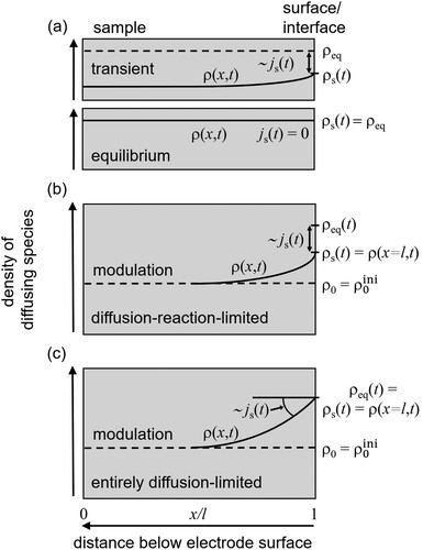
Figure 1. Schematic display of the solute density, $\rho (x,t)$, inside the sample during hydrogen charging (a) and subsequent modulation (b). (a) Applying a constant electrode potential $U=U_0$ for a sufficient time interval leads to a homogeneous hydrogen concentration ${\rho }_{\mathrm{eq}}$ inside the sample. Before equilibrium is reached, the difference ${\rho }_{\mathrm{eq}}-{\rho }_s$ results in a current density $j_{\mathrm{s}}\left(t\right)$, Equation (10(10) $j_{\mathrm{s}}=\frac{j_{\mathrm{ex}}}{{\rho }_{\mathrm{eq}}}({\rho }_{\mathrm{eq}}-{\rho }_{\mathrm{s}}).$(10) ), of solutes through the surface, where ${\rho }_s$ is the time-dependent density underneath the surface. (b) After reaching equilibrium, the electrode potential $U\left(t\right)$, Equation (2(2) $U\left(t\right)=U_0+\hat{U}\sin \left(\mathrm{\omega t}\right),$(2) ), is modulated with respect to $U_0$ giving rise to an oscillating variation of the solute density imposed by the surface, ${\rho }_{\mathrm{eq}}\left(t\right)={\rho }_0+\hat{\rho }\sin \left(\mathrm{\omega t}\right)$, Equation (11(11) ${\rho }_{\mathrm{eq}}\left(t\right)={\rho }_0+\hat{\rho }\sin \mathrm{\omega t}={\rho }_0(1-\frac{\mathrm{zF}}{\mathrm{RT}}\hat{U}\sin \mathrm{\omega t}),$(11) ). As a result of the modulation, a time-dependent density profile, $\rho (x,t)$, inside the sample evolves, which is determined by the reaction- and diffusion-limitation of the process, Section 2.3. The difference between ${\rho }_{\mathrm{eq}}\left(t\right)$ and ${\rho }_s\left(t\right)=\rho (x=l,t)$ leads again to a current density $j_{\mathrm{s}}\left(t\right)$ of particles through the surface (Equation (12(12) $j_{\mathrm{s}}\left(t\right)=\frac{j_{\mathrm{ex}}}{{\rho }_0}\left({\rho }_{\mathrm{eq}}\right(t)-\rho (l,t\left)\right),$(12) ) and boundary condition according to Equation (14(14) ${D\frac{\mathrm{\partial }\rho (x,t)}{\mathrm{\partial }x}|}_{x=l}=\kappa \left({\rho }_{\mathrm{eq}}\right(t)-\rho (l,t\left)\right),$(14) )). (c) In comparison to (b) the situation for the entirely diffusion-limited case (boundary condition according to Equation (16(16) $\rho (x=l,t)={\rho }_0+\hat{\rho }\sin \left(\mathrm{\omega t}\right)$(16) )). Note that figure parts b and c pertain to the special case of the diffusion–reaction model with the initial condition, Equation (18(18) $\rho (t=0)={\rho }_0^{\mathrm{ini}}.$(18) ), $\rho (t=0)={\rho }_0^{\mathrm{ini}}={\rho }_0$.

Before the start of the experiment, a constant electrode potential is applied during a time interval sufficient for the composition profile in the solid to reach equilibrium. This leads to a homogeneous concentration throughout the solid. The experiment proper consists in imposing a finite mean value, $U_0$, of the electrode potential, to which a small modulation is superimposed, so that the time-dependent potential is (2) $U\left(t\right)=U_0+\hat{U}\sin \left(\mathrm{\omega t}\right),$(2) with the amplitude $\hat{U}$, the radian frequency ω and the time t.

2.1.2. Relation between chemical potential, concentration and applied potential

The modulation of $U\left(t\right)$ implies a modulation of the solute concentration ${\rho }_{\mathrm{eq}}$ in the solid crystal at equilibrium. Empirical data for the equation of state, $\breve{\mu }(\rho ,T)$, for the chemical potential of hydrogen as the function of ρ and temperature T have been well documented for many metal hydrides. For the example of Pd, as a standard model system and one of the most extensively studied hydrides, the equation of state reflects a miscibility gap separating a dilute from a concentrated solid solution below the critical temperature of ∼ 570 K [5–8]. Here, we ignore the phase separation and the underlying hydrogen–hydrogen interaction in more concentrated solutions and we restrict attention, instead, to situations where the solute fraction remains within the dilute limit at any position and any time. At equilibrium, μ and ρ are then related through the dilute solution equation of state [9] (3) $\breve{\mu }(\rho ,T)={\mu }_{\mathrm{ref}}+\mathrm{RTln}\left(\frac{\rho }{{\rho }_{\mathrm{ref}}}\right)$(3) with ${\mu }_{\mathrm{ref}}$ and ${\rho }_{\mathrm{ref}}$ the chemical potential and the solute concentration, respectively, at equilibrium in a suitably defined, dilute reference state.

The equilibrium chemical potential of atomic hydrogen in the solid can be controlled by the electrode potential, U, according to (4) ${\mu }_{\mathrm{eq}}={\mu }_{\mathrm{ref}}-\mathrm{zF}(U-U_{\mathrm{ref}}).$(4) Here z is the signed valency, z = +1 for protons, F is Faraday's constant, and $U_{\mathrm{ref}}$ is the electrode potential required to maintain the reference state. Equations (3(3) $\breve{\mu }(\rho ,T)={\mu }_{\mathrm{ref}}+\mathrm{RTln}\left(\frac{\rho }{{\rho }_{\mathrm{ref}}}\right)$(3) ) and (4(4) ${\mu }_{\mathrm{eq}}={\mu }_{\mathrm{ref}}-\mathrm{zF}(U-U_{\mathrm{ref}}).$(4) ) imply (5) $\breve{\rho }(U,T)={\rho }_{\mathrm{ref}}\exp (-\frac{\mathrm{zF}(U-U_{\mathrm{ref}})}{\mathrm{RT}})$(5) (6) $\breve{U}(\rho ,T)=U_{\mathrm{ref}}-\frac{\mathrm{zF}}{\mathrm{RT}}\ln \left(\frac{\rho }{{\rho }_{\mathrm{ref}}}\right)$(6) as two forms of equilibrium sorption isotherms, in other words, of equations of state governing the relation between the solute concentration and the electrode potential at equilibrium.

2.2. Boundary condition at the electrode surface

2.2.1. Current-overpotential equation

We require a rate equation for the flux density, $j_{\mathrm{s}}$, of transfer from the electrolyte into the solid crystal. As stated above, we assume an energy barrier at the interface. The rate of transfer across the interface may then be inferred from kinetic rate theory.

Prior to discussing the kinetics, we find it useful to inspect the nature of the underlying equilibrium states, presented in Figure 1(a). Consider that electrolyte and hydride have been equilibrated during a sufficient hold time at a constant but otherwise arbitrary electrode potential $U_0$. The bulk of the hydride will then have reached an equilibrium state, which is at constant composition ${\rho }_{\mathrm{eq}}$. Specifically, the composition at the surface also satisfies ${\rho }_s={\rho }_{\mathrm{eq}}$. In this state, $j_{\mathrm{s}}$ is zero (see Figure 1(a), lower part). In other words, and contrary to simple electrode reactions, there is not a single value of the equilibrium potential but rather a continuum of possible equilibrium states with combinations of electrode potential (or chemical potential) and solid solution concentration that are governed by the bulk sorption isotherm. Non-zero values of the flux $j_{\mathrm{s}}$ result whenever the combination of U and ${\rho }_s$ deviates from the isotherm.

Outside equilibrium, the flux $j_{\mathrm{s}}$ will be governed by a Butler-Volmer-like current-overpotential equation (see Sect 3.4.2 in Ref. [3]). That equation must embody that the rates of injection and extraction scale with the concentrations of vacant target and of occupied starting sites in the crystal, respectively [10]. In other words, the kinetics is affected by the time-dependent concentrations of i and H in Equation (1(1) ${\mathrm{H}}^{+}+{\mathrm{e}}^{-}+\mathrm{i}\leftrightarrows \mathrm{H}.$(1) ); those concentrations add up to the constant site density ${\rho }_{\mathrm{site}}$. Furthermore, as discussed above, the equation must also embody that the flux vanishes at equilibrium at any imposed potential $U_{\mathrm{eq}}$, in other words, that $j_{\mathrm{s}}=0$ when ${\rho }_s={\rho }_{\mathrm{eq}}=\breve{\rho }(U_{\mathrm{eq}},T)$. The current-potential relation may thus be written as (7) $j_{\mathrm{s}}=j_{\mathrm{ex}}[\frac{{\rho }_{\mathrm{site}}-{\rho }_{\mathrm{s}}}{{\rho }_{\mathrm{site}}-{\rho }_{\mathrm{eq}}}\exp (-\alpha \frac{\mathrm{zF}(U-U_{\mathrm{eq}})}{\mathrm{RT}})-\frac{{\rho }_{\mathrm{s}}}{{\rho }_{\mathrm{eq}}}\exp \left(\right(1-\alpha \left)\frac{\mathrm{zF}(U-U_{\mathrm{eq}})}{\mathrm{RT}}\right)],$(7) with α the transfer coefficient and $j_{\mathrm{ex}}$ the exchange current density [3].

As the discussion that leads to Equation (7(7) $j_{\mathrm{s}}=j_{\mathrm{ex}}[\frac{{\rho }_{\mathrm{site}}-{\rho }_{\mathrm{s}}}{{\rho }_{\mathrm{site}}-{\rho }_{\mathrm{eq}}}\exp (-\alpha \frac{\mathrm{zF}(U-U_{\mathrm{eq}})}{\mathrm{RT}})-\frac{{\rho }_{\mathrm{s}}}{{\rho }_{\mathrm{eq}}}\exp \left(\right(1-\alpha \left)\frac{\mathrm{zF}(U-U_{\mathrm{eq}})}{\mathrm{RT}}\right)],$(7) ) imposes no restriction on the choice (precise value of $U_{\mathrm{eq}}$ or ${\rho }_{\mathrm{eq}}$) of the equilibrium state, one may arbitrarily select that state as long as it remains within the dilute limit, as supposed above. In particular, setting either ${\rho }_{\mathrm{eq}}={\rho }_s$ or alternatively $U_{\mathrm{eq}}=U$ are two distinct and valid choices. The former choice leads to the standard form of the Butler-Volmer equation, namely (8) $j_{\mathrm{s}}=j_{\mathrm{ex}}[\exp (-\alpha \frac{\mathrm{zF\delta U}}{\mathrm{RT}})-\exp \left(\right(1-\alpha \left)\frac{\mathrm{zF\delta U}}{\mathrm{RT}}\right)]$(8) where $\mathrm{\delta U}$ denotes an overpotential relative to the equilibrium electrode potential for the current surface concentration value, $\mathrm{\delta U}=U-\breve{U}({\rho }_s,T)$. The latter choice leads to (9) $j_{\mathrm{s}}=j_{\mathrm{ex}}(\frac{{\rho }_{\mathrm{site}}-{\rho }_{\mathrm{s}}}{{\rho }_{\mathrm{site}}-{\rho }_{\mathrm{eq}}}-\frac{{\rho }_{\mathrm{s}}}{{\rho }_{\mathrm{eq}}}).$(9) where ${\rho }_{\mathrm{eq}}$ is the equilibrium concentration at the current electrode potential value, ${\rho }_{\mathrm{eq}}=\breve{\rho }(U,T)$. It is emphasised that each of the two Equations (8(8) $j_{\mathrm{s}}=j_{\mathrm{ex}}[\exp (-\alpha \frac{\mathrm{zF\delta U}}{\mathrm{RT}})-\exp \left(\right(1-\alpha \left)\frac{\mathrm{zF\delta U}}{\mathrm{RT}}\right)]$(8) ) and (9(9) $j_{\mathrm{s}}=j_{\mathrm{ex}}(\frac{{\rho }_{\mathrm{site}}-{\rho }_{\mathrm{s}}}{{\rho }_{\mathrm{site}}-{\rho }_{\mathrm{eq}}}-\frac{{\rho }_{\mathrm{s}}}{{\rho }_{\mathrm{eq}}}).$(9) ), are equivalent formulations for the flux that embody the same physics. Since our approach to the diffusion kinetics in the bulk naturally connects to ${\rho }_s$ as a key variable in the boundary condition for diffusion, we here choose the latter expression, Equation (9(9) $j_{\mathrm{s}}=j_{\mathrm{ex}}(\frac{{\rho }_{\mathrm{site}}-{\rho }_{\mathrm{s}}}{{\rho }_{\mathrm{site}}-{\rho }_{\mathrm{eq}}}-\frac{{\rho }_{\mathrm{s}}}{{\rho }_{\mathrm{eq}}}).$(9) ), as the convenient governing law for the flux through the interface.

For dilute solutions ($\rho \ll {\rho }_{\mathrm{site}}$), Equation (9(9) $j_{\mathrm{s}}=j_{\mathrm{ex}}(\frac{{\rho }_{\mathrm{site}}-{\rho }_{\mathrm{s}}}{{\rho }_{\mathrm{site}}-{\rho }_{\mathrm{eq}}}-\frac{{\rho }_{\mathrm{s}}}{{\rho }_{\mathrm{eq}}}).$(9) ) can be simplified to (10) $j_{\mathrm{s}}=\frac{j_{\mathrm{ex}}}{{\rho }_{\mathrm{eq}}}({\rho }_{\mathrm{eq}}-{\rho }_{\mathrm{s}}).$(10) This result confirms the linear dependence of $j_{\mathrm{s}}$ on the surface solute fraction as derived in [10]. Equation (10(10) $j_{\mathrm{s}}=\frac{j_{\mathrm{ex}}}{{\rho }_{\mathrm{eq}}}({\rho }_{\mathrm{eq}}-{\rho }_{\mathrm{s}}).$(10) ) shows that, at any given value of the electrode potential (as parameterised by the value of ${\rho }_{\mathrm{eq}}$ along with Equation (6(6) $\breve{U}(\rho ,T)=U_{\mathrm{ref}}-\frac{\mathrm{zF}}{\mathrm{RT}}\ln \left(\frac{\rho }{{\rho }_{\mathrm{ref}}}\right)$(6) )), the flux through the interface is a linear function of the surface composition, with zero current at equilibrium. Note that the linearity persists even for finite deviations of the surface composition from equilibrium. Equation (10(10) $j_{\mathrm{s}}=\frac{j_{\mathrm{ex}}}{{\rho }_{\mathrm{eq}}}({\rho }_{\mathrm{eq}}-{\rho }_{\mathrm{s}}).$(10) ) derived above for the time-independent equilibrium (${\rho }_{\mathrm{eq}}$) holds also for the time-dependent equilibrium.

2.2.2. Application to experiments with modulated electrode potential and connection to bulk diffusion problem

In the following, the general form of the current density, Equation (10(10) $j_{\mathrm{s}}=\frac{j_{\mathrm{ex}}}{{\rho }_{\mathrm{eq}}}({\rho }_{\mathrm{eq}}-{\rho }_{\mathrm{s}}).$(10) ), obtained from the Butler–Volmer equation, will be specified to the experimental situation under consideration, Figure 1(b), in order to determine the boundary condition for the diffusion–reaction model treated in the next Section 2.3. As stated in the previous Section 2.2.1, the solid is initially equilibrated at a homogeneous concentration ${\rho }_{\mathrm{eq}}$ by holding the electrode potential at a constant value $U_0$. This corresponds to the situation depicted in the lower part of Figure 1(a). From t = 0 onwards a small cyclic potential variation of amplitude $\hat{U}$ is superimposed.

Equation (5(5) $\breve{\rho }(U,T)={\rho }_{\mathrm{ref}}\exp (-\frac{\mathrm{zF}(U-U_{\mathrm{ref}})}{\mathrm{RT}})$(5) ) implies that the potential variation entails a cyclic variation of the equilibrium concentration value around its mean value, ${\rho }_0$. If that variation is small, $\mathrm{zF}\hat{U}\ll \mathrm{RT}$, the exponential can be linearised and one obtains the equilibrium concentration (11) ${\rho }_{\mathrm{eq}}\left(t\right)={\rho }_0+\hat{\rho }\sin \mathrm{\omega t}={\rho }_0(1-\frac{\mathrm{zF}}{\mathrm{RT}}\hat{U}\sin \mathrm{\omega t}),$(11) with $\hat{\rho }$ a modulation amplitude.

The modulation of ${\rho }_{\mathrm{eq}}\left(t\right)$, Equation (11(11) ${\rho }_{\mathrm{eq}}\left(t\right)={\rho }_0+\hat{\rho }\sin \mathrm{\omega t}={\rho }_0(1-\frac{\mathrm{zF}}{\mathrm{RT}}\hat{U}\sin \mathrm{\omega t}),$(11) ), results in a current according to Equation (10(10) $j_{\mathrm{s}}=\frac{j_{\mathrm{ex}}}{{\rho }_{\mathrm{eq}}}({\rho }_{\mathrm{eq}}-{\rho }_{\mathrm{s}}).$(10) ) (see scheme, Figure 1(b)): (12) $j_{\mathrm{s}}\left(t\right)=\frac{j_{\mathrm{ex}}}{{\rho }_0}\left({\rho }_{\mathrm{eq}}\right(t)-\rho (l,t\left)\right),$(12) with ${\rho }_s$ given by the solution $\rho (x=l,t)$ of the diffusion–reaction model. In Equation (12(12) $j_{\mathrm{s}}\left(t\right)=\frac{j_{\mathrm{ex}}}{{\rho }_0}\left({\rho }_{\mathrm{eq}}\right(t)-\rho (l,t\left)\right),$(12) ), a simplification has been considered by exploiting $\delta {\rho }_{\mathrm{eq}}={\rho }_{\mathrm{eq}}\left(t\right)-{\rho }_0\ll {\rho }_0$. In fact, replacing the time-dependent ${\rho }_{\mathrm{eq}}\left(t\right)$ in the denominator of the prefactor, Equation (10(10) $j_{\mathrm{s}}=\frac{j_{\mathrm{ex}}}{{\rho }_{\mathrm{eq}}}({\rho }_{\mathrm{eq}}-{\rho }_{\mathrm{s}}).$(10) ), with the constant ${\rho }_0$ affects the result only by terms in second order ($\propto \delta {\rho }_{\mathrm{eq}}\delta {\rho }_{\mathrm{s}}$), which can be neglected.

This result for the current density $j_{\mathrm{s}}$ of particles through the surface, Equation (12(12) $j_{\mathrm{s}}\left(t\right)=\frac{j_{\mathrm{ex}}}{{\rho }_0}\left({\rho }_{\mathrm{eq}}\right(t)-\rho (l,t\left)\right),$(12) ), provides the surface condition, i.e. the boundary condition for the bulk diffusion problem. The current density through the surface is linked to the bulk concentration profile by (13) $j_{\mathrm{s}}\left(t\right)={-D\frac{\mathrm{\partial }\rho (x,t)}{\mathrm{\partial }x}|}_{x=l},$(13) where D denotes the diffusion coefficient of the solute in the solid crystal. In the previous part of this subsection, positive values of $j_{\mathrm{s}}$ correspond to injection of solute into the sample, associated with ${\rho }_{\mathrm{eq}}\left(t\right)>\rho (l,t)$. In the bulk-diffusion model with the surface located at x = l, however, a particle current into the sample according to Equation (13(13) $j_{\mathrm{s}}\left(t\right)={-D\frac{\mathrm{\partial }\rho (x,t)}{\mathrm{\partial }x}|}_{x=l},$(13) ) correspond to negative values of $j_{\mathrm{s}}$ (see Figure 1). Taking this into account, one obtains from Equations (12(12) $j_{\mathrm{s}}\left(t\right)=\frac{j_{\mathrm{ex}}}{{\rho }_0}\left({\rho }_{\mathrm{eq}}\right(t)-\rho (l,t\left)\right),$(12) ) and (13(13) $j_{\mathrm{s}}\left(t\right)={-D\frac{\mathrm{\partial }\rho (x,t)}{\mathrm{\partial }x}|}_{x=l},$(13) ) the boundary condition at the electrode surface: (14) ${D\frac{\mathrm{\partial }\rho (x,t)}{\mathrm{\partial }x}|}_{x=l}=\kappa \left({\rho }_{\mathrm{eq}}\right(t)-\rho (l,t\left)\right),$(14) where the ratio (15) $\kappa =\frac{j_{\mathrm{ex}}}{{\rho }_0}$(15) describes the reaction rate. Note that the exchange current density $j_{\mathrm{ex}}$ is proportional to the mean value of ${\rho }_0$ of the cyclic variation of the equilibrium concentration value, which is well in line with literature (see Section 3.4.1 in Ref. [3]). The obtained boundary condition, Equation (14(14) ${D\frac{\mathrm{\partial }\rho (x,t)}{\mathrm{\partial }x}|}_{x=l}=\kappa \left({\rho }_{\mathrm{eq}}\right(t)-\rho (l,t\left)\right),$(14) ), corresponds to standard diffusion–reaction theory (Equation (5.45) in Ref. [11]).

With increasing reaction rate, the value $\rho (l,t)$ more and more approaches the equilibrium concentration ${\rho }_{\mathrm{eq}}\left(t\right)$, Equation (11(11) ${\rho }_{\mathrm{eq}}\left(t\right)={\rho }_0+\hat{\rho }\sin \mathrm{\omega t}={\rho }_0(1-\frac{\mathrm{zF}}{\mathrm{RT}}\hat{U}\sin \mathrm{\omega t}),$(11) ), imposed by the surface, leading to the boundary condition (16) $\rho (x=l,t)={\rho }_0+\hat{\rho }\sin \left(\mathrm{\omega t}\right)$(16) in the entirely diffusion-limited regime with the current density according to Equation (13(13) $j_{\mathrm{s}}\left(t\right)={-D\frac{\mathrm{\partial }\rho (x,t)}{\mathrm{\partial }x}|}_{x=l},$(13) ). The scheme of this boundary condition is shown in Figure 1(c) for comparison with that in Figure 1(b) for the boundary condition associated with the reaction rate, Equation (14(14) ${D\frac{\mathrm{\partial }\rho (x,t)}{\mathrm{\partial }x}|}_{x=l}=\kappa \left({\rho }_{\mathrm{eq}}\right(t)-\rho (l,t\left)\right),$(14) ). As shown in Subsection 3.2, the present diffusion–reaction model contains the entirely diffusion-limited regime as special case.

2.3. Diffusion model with modulated boundary condition

In the following section, the bulk-diffusion problem is solved in order to determine the spatial and temporal variation of the density of diffusion species $\rho (x,t)$ and the current density $j_{\mathrm{s}}$ through the surface (see scheme in Figure 1). In addition to the planar electrode, Section 2.3.1, the cylindical-shaped electrode is considered, Section 2.3.2.

2.3.1. Solution for one-dimensional case: planar electrode

The diffusion equation in one dimension for a plate with thickness $2l$ ($-l\le x\le l$) is of interest here. In the bulk it is given by (17) $\frac{\mathrm{\partial }\rho }{\mathrm{\partial }t}=D\frac{{\mathrm{\partial }}^2\rho }{\mathrm{\partial }{x}^2}.$(17) As initial condition within the plate (t = 0, $-l\le x\le l$) a homogeneous distribution is assumed: (18) $\rho (t=0)={\rho }_0^{\mathrm{ini}}.$(18) The boundary condition for the surface (x = l) is given by Equation (14(14) ${D\frac{\mathrm{\partial }\rho (x,t)}{\mathrm{\partial }x}|}_{x=l}=\kappa \left({\rho }_{\mathrm{eq}}\right(t)-\rho (l,t\left)\right),$(14) ), which reads with ${\rho }_{\mathrm{eq}}\left(t\right)$ according to Equation (11(11) ${\rho }_{\mathrm{eq}}\left(t\right)={\rho }_0+\hat{\rho }\sin \mathrm{\omega t}={\rho }_0(1-\frac{\mathrm{zF}}{\mathrm{RT}}\hat{U}\sin \mathrm{\omega t}),$(11) ): (19) ${D\frac{\mathrm{\partial }\rho }{\mathrm{\partial }x}|}_{x=l}=\kappa ({\rho }_0+\hat{\rho }\sin (\mathrm{\omega t})-\rho (l\left)\right).$(19) Note that the initial condition, Equation (18(18) $\rho (t=0)={\rho }_0^{\mathrm{ini}}.$(18) ), is more general than the scenario depicted in Figure 1(b), where as initial condition, Equation (18(18) $\rho (t=0)={\rho }_0^{\mathrm{ini}}.$(18) ), $\rho (t=0)={\rho }_0$, i.e. ${\rho }_0^{\mathrm{ini}}={\rho }_0$, is assumed. Therefore, the present model also takes into account the transient during which the concentration field approaches the value ${\rho }_0$ with respect to which the modulation occurs. The special case ${\rho }_0^{\mathrm{ini}}={\rho }_0$ will be considered in the analysis (see Section 3.4).

The condition of vanishing flux in the midplane of the plate defines another boundary condition for x = 0: (20) ${\frac{\mathrm{\partial }\rho }{\mathrm{\partial }x}|}_{x=0}=0.$(20) Handling the time dependence by the Laplace transform (21) $\tilde{\rho }(x,p)={\int }_0^{\mathrm{\infty }}\exp (-\mathrm{pt})\rho (x,t)\mathrm{d}t,$(21) the diffusion equation with initial condition is given by: (22) $\frac{{\mathrm{d}}^2\tilde{\rho }}{\mathrm{d}{\mathrm{x}}^2}-{\gamma }^2\tilde{\rho }=-\frac{{\rho }_0^{\mathrm{ini}}}{D}\mathrm{with}{\gamma }^2=\frac{p}{D}.$(22) For the Laplace transform of the boundary condition one obtains with $\sin \left(\mathrm{\omega t}\right)\to \omega /(p^2+{\omega }^2)$: (23) ${D\frac{\mathrm{d}\tilde{\rho }}{\mathrm{d}x}|}_{x=l}=\kappa (\frac{{\rho }_0}{p}+\hat{\rho }\frac{\omega }{p^2+{\omega }^2}-\tilde{\rho }(l\left)\right).$(23) The solution of the diffusion equation (Equation (22(22) $\frac{{\mathrm{d}}^2\tilde{\rho }}{\mathrm{d}{\mathrm{x}}^2}-{\gamma }^2\tilde{\rho }=-\frac{{\rho }_0^{\mathrm{ini}}}{D}\mathrm{with}{\gamma }^2=\frac{p}{D}.$(22) )) with the boundary conditions for x = 0, Equation (20(20) ${\frac{\mathrm{\partial }\rho }{\mathrm{\partial }x}|}_{x=0}=0.$(20) ), and x = l, Equation (23(23) ${D\frac{\mathrm{d}\tilde{\rho }}{\mathrm{d}x}|}_{x=l}=\kappa (\frac{{\rho }_0}{p}+\hat{\rho }\frac{\omega }{p^2+{\omega }^2}-\tilde{\rho }(l\left)\right).$(23) ), reads (see Appendix A.1): (24) $\tilde{\rho }(x,p)=\frac{L({\rho }_0-{\rho }_0^{\mathrm{ini}})\cosh \left(\mathrm{\gamma x}\right)}{p(\mathrm{Lcosh}\text{β}+\text{β}\sinh \text{β})}+\frac{{\rho }_0^{\mathrm{ini}}}{p}+\hat{\rho }\frac{\mathrm{L\omega cosh}\left(\mathrm{\gamma x}\right)}{(p^2+{\omega }^2)(\mathrm{Lcosh}\text{β}+\text{β}\sinh \text{β})},$(24) with $\text{β}=\mathrm{\gamma l}$, ${\text{β}}^2=p{l}^2/D$, and the parameter (25) $L=\frac{\mathrm{\kappa l}}{D},$(25) which characterises the ratio between diffusion ($\propto l/D$) and reaction ($\propto 1/\kappa$) limitation. The retransformation $\tilde{\rho }(x,p)\to \rho (x,t)$ is given in Appendix A.1.

In the following, we are primarily interested in the volume-averaged time-dependent fraction of loaded species (26) $n\left(t\right)=\frac{A^{\prime }}{{\rho }_0{A}^{\prime }l}{\int }_0^l\rho (x,t)\mathrm{d}x$(26) and the particle current density through the surface, which is associated with the time-derivative of $n\left(t\right)$, i.e. (27) $j_{\mathrm{s}}=-\frac{{\rho }_0{A}^{\prime }l}{A^{\prime }}\frac{\mathrm{d}n}{\mathrm{d}t}$(27) with the electrode area $A^{\prime }$. Note the minus-sign since the current density through the surface at x = l, Equation (13(13) $j_{\mathrm{s}}\left(t\right)={-D\frac{\mathrm{\partial }\rho (x,t)}{\mathrm{\partial }x}|}_{x=l},$(13) ), is negative for $\mathrm{d}n/\mathrm{d}t>0$.¹

With $\rho (x,t)$ as sum of Equations (A3(A3) ${\rho }_{\mathrm{unmod}}(x,t)={\rho }_0[1-\frac{{\rho }_0-{\rho }_0^{\mathrm{ini}}}{{\rho }_0}\sum _{n=1}^{\mathrm{\infty }}\frac{2\mathrm{Lcos}\left({\overline{\text{β}}}_{n}x/l\right)}{\cos {\overline{\text{β}}}_n({\overline{\text{β}}}_n^2+L^2+L)}\exp (-\frac{D{\overline{\text{β}}}_n^2}{l^2}t)]$(A3) ), (A6(A6) ${\rho }_{\mathrm{mod}}^{\mathrm{transient}}(x,t)=\sum _{n=1}^{\mathrm{\infty }}\frac{1}{2}\hat{\rho }\frac{M^2{\overline{\text{β}}}_n^2}{{\overline{\text{β}}}_n^4+\frac{1}{4}{M}^4}\frac{2\mathrm{Lcos}\left(\overline{\text{β}}x/l\right)}{\cos {\overline{\text{β}}}_n({\overline{\text{β}}}_n^2+L^2+L)}\exp (-\frac{D{\overline{\text{β}}}_n^2}{l^2}t)$(A6) ), and (A9(A9) ${\rho }_{\mathrm{mod}}^{\mathrm{periodic}}(x,t)=\frac{\hat{\rho }\mathrm{Lcos}\left({\overline{\text{β}}}_{+}x/l\right)\exp \left(\mathrm{i\omega t}\right)}{2i(\mathrm{Lcos}{\overline{\text{β}}}_{+}-{\overline{\text{β}}}_{+}\sin {\overline{\text{β}}}_{+})}-\frac{\hat{\rho }\mathrm{Lcos}\left({\overline{\text{β}}}_{-}x/l\right)\exp (-\mathrm{i\omega t})}{2i(\mathrm{Lcos}{\overline{\text{β}}}_{-}-{\overline{\text{β}}}_{-}\sin {\overline{\text{β}}}_{-})}$(A9) ) one obtains (28) $\begin{array}{rl}n\left(t\right)& =1-\sum _{n=1}^{\mathrm{\infty }}\frac{2L^2}{{\overline{\text{β}}}_n^2({\overline{\text{β}}}_n^2+L^2+L)}[\frac{{\rho }_0-{\rho }_0^{\mathrm{ini}}}{{\rho }_0}-\frac{1}{2}\frac{\hat{\rho }}{{\rho }_0}\frac{M^2{\overline{\text{β}}}_n^2}{{\overline{\text{β}}}_n^4+\frac{1}{4}{M}^4}]\exp (-\frac{D{\overline{\text{β}}}_n^2}{l^2}t)\\ & +2\frac{\hat{\rho }}{{\rho }_0}\frac{L}{M}\frac{C}{\sqrt{A^2+B^2}}\sin (\mathrm{\omega t}+{\varphi }_0)\end{array}$(28) and (29) $\begin{array}{rl}{j}_{\mathrm{s}}& =\sum _{n=1}^{\mathrm{\infty }}\frac{2\mathrm{L\kappa }}{({\overline{\text{β}}}_n^2+L^2+L)}[{\rho }_0^{\mathrm{ini}}-{\rho }_0+\frac{1}{2}\hat{\rho }\frac{M^2{\overline{\text{β}}}_n^2}{{\overline{\text{β}}}_n^4+\frac{1}{4}{M}^4}]\exp (-\frac{D{\overline{\text{β}}}_n^2}{l^2}t)\\ & -2l\hat{\rho }\frac{\mathrm{L\omega }}{M}\frac{C}{\sqrt{A^2+B^2}}\sin (\mathrm{\omega t}+{\varphi }_0+\frac{\pi }{2}),\end{array}$(29) with L according to Equation (25(25) $L=\frac{\mathrm{\kappa l}}{D},$(25) ), with the modulation-characterising parameter (30) $M=\sqrt{\frac{2l^2\omega }{D}},$(30) with the roots ${\overline{\text{β}}}_n$ according to (31) ${\overline{\text{β}}}_n\tan {\overline{\text{β}}}_n=L,$(31) and with the phase angle (32) ${\varphi }_0=\arctan \frac{A}{B}+0\text{or}\pi$(32) (0 for B > 0 and π for B < 0) with the coefficients (33) $\begin{array}{rl}A& =L(\sin M-\sinh M)+M(\cos M-\cosh M),\\ B& =L(\sin M+\sinh M),\\ C& =\cosh M-\cos M.\end{array}$(33) Note that the fraction $n\left(t\right)$ is normalised with respect to the mean value ${\rho }_0$ in the surrounding.

Both the fraction $n\left(t\right)$, Equation (28(28) $\begin{array}{rl}n\left(t\right)& =1-\sum _{n=1}^{\mathrm{\infty }}\frac{2L^2}{{\overline{\text{β}}}_n^2({\overline{\text{β}}}_n^2+L^2+L)}[\frac{{\rho }_0-{\rho }_0^{\mathrm{ini}}}{{\rho }_0}-\frac{1}{2}\frac{\hat{\rho }}{{\rho }_0}\frac{M^2{\overline{\text{β}}}_n^2}{{\overline{\text{β}}}_n^4+\frac{1}{4}{M}^4}]\exp (-\frac{D{\overline{\text{β}}}_n^2}{l^2}t)\\ & +2\frac{\hat{\rho }}{{\rho }_0}\frac{L}{M}\frac{C}{\sqrt{A^2+B^2}}\sin (\mathrm{\omega t}+{\varphi }_0)\end{array}$(28) ), and the associated current density $j_{\mathrm{s}}$, Equation (29(29) $\begin{array}{rl}{j}_{\mathrm{s}}& =\sum _{n=1}^{\mathrm{\infty }}\frac{2\mathrm{L\kappa }}{({\overline{\text{β}}}_n^2+L^2+L)}[{\rho }_0^{\mathrm{ini}}-{\rho }_0+\frac{1}{2}\hat{\rho }\frac{M^2{\overline{\text{β}}}_n^2}{{\overline{\text{β}}}_n^4+\frac{1}{4}{M}^4}]\exp (-\frac{D{\overline{\text{β}}}_n^2}{l^2}t)\\ & -2l\hat{\rho }\frac{\mathrm{L\omega }}{M}\frac{C}{\sqrt{A^2+B^2}}\sin (\mathrm{\omega t}+{\varphi }_0+\frac{\pi }{2}),\end{array}$(29) ), are composed of three parts, namely

• the unmodulated part given by the respective term associated with $({\rho }_0-{\rho }_0^{\mathrm{ini}})$ in the ${\overline{\text{β}}}_n$-series, which is identical to that given in textbook (Equation (4.53) in Ref. [11] as well as Equation (19) in Ref. [2] and Equation (28) in Ref. [10]), and which is also in line with measurements conducted with the potential step method (see Section 3.6 for further details),

• the transient part upon starting the modulaton given by the additional summand $\propto \hat{\rho }$ in the ${\overline{\text{β}}}_n$-series, and

• the temporally periodic part associated with the modulation.

An analysis of $n\left(t\right)$ will be given in Sections 3.2 and 3.3.

For the sake of completeness we quote exemplary for the one-dimensional case, how the oscillating boundary condition spatially evolves within the plate. The dependence of the density of loaded species $\rho (x,t)$ on t and x is given by the sum (34) $\rho (x,t)={\rho }_{\mathrm{unmod}}(x,t)+{\rho }_{\mathrm{mod}}^{\mathrm{transient}}(x,t)+{\rho }_{\mathrm{mod}}^{\mathrm{periodic}}(x,t),$(34) which consists of three parts in an analogous manner to $n\left(t\right)$ or $j_{\mathrm{s}}$ that follow from $\rho (x,t)$: the unmodulated part ${\rho }_{\mathrm{unmod}}(x,t)$, Equation (A3(A3) ${\rho }_{\mathrm{unmod}}(x,t)={\rho }_0[1-\frac{{\rho }_0-{\rho }_0^{\mathrm{ini}}}{{\rho }_0}\sum _{n=1}^{\mathrm{\infty }}\frac{2\mathrm{Lcos}\left({\overline{\text{β}}}_{n}x/l\right)}{\cos {\overline{\text{β}}}_n({\overline{\text{β}}}_n^2+L^2+L)}\exp (-\frac{D{\overline{\text{β}}}_n^2}{l^2}t)]$(A3) ), the transient ${\rho }_{\mathrm{mod}}^{\mathrm{transient}}(x,t)$, Equation (A6(A6) ${\rho }_{\mathrm{mod}}^{\mathrm{transient}}(x,t)=\sum _{n=1}^{\mathrm{\infty }}\frac{1}{2}\hat{\rho }\frac{M^2{\overline{\text{β}}}_n^2}{{\overline{\text{β}}}_n^4+\frac{1}{4}{M}^4}\frac{2\mathrm{Lcos}\left(\overline{\text{β}}x/l\right)}{\cos {\overline{\text{β}}}_n({\overline{\text{β}}}_n^2+L^2+L)}\exp (-\frac{D{\overline{\text{β}}}_n^2}{l^2}t)$(A6) ), associated with the modulated part, and the spatially and temporally oscillating part given by (see Appendix A.1.2) (35) ${\rho }_{\mathrm{mod}}^{\mathrm{periodic}}(x,t)=2\hat{\rho }L\sqrt{\frac{P_1^2+P_2^2}{R_1^2+R_2^2}}\sin (\mathrm{\omega t}+{\varphi }_0)$(35) with (36) $\tan {\varphi }_0=\frac{R_2{P}_2-R_1{P}_1}{R_1{P}_2+R_2{P}_1}+0,\pi$(36) and (37) $\begin{array}{rl}m& =\frac{M}{2l},\\ P_1& =\cos \left(\mathrm{mx}\right)\cosh \left(\mathrm{mx}\right),\\ P_2& =\sin \left(\mathrm{mx}\right)\sinh \left(\mathrm{mx}\right),\\ R_1& =2\mathrm{Lsin}\frac{M}{2}\sinh \frac{M}{2}+M(\sin \frac{M}{2}\cosh \frac{M}{2}+\cos \frac{M}{2}\sinh \frac{M}{2}),\\ R_2& =2\mathrm{Lcos}\frac{M}{2}\cosh \frac{M}{2}+M(-\sin \frac{M}{2}\cosh \frac{M}{2}+\cos \frac{M}{2}\sinh \frac{M}{2}).\end{array}$(37) With Equation (37(37) $\begin{array}{rl}m& =\frac{M}{2l},\\ P_1& =\cos \left(\mathrm{mx}\right)\cosh \left(\mathrm{mx}\right),\\ P_2& =\sin \left(\mathrm{mx}\right)\sinh \left(\mathrm{mx}\right),\\ R_1& =2\mathrm{Lsin}\frac{M}{2}\sinh \frac{M}{2}+M(\sin \frac{M}{2}\cosh \frac{M}{2}+\cos \frac{M}{2}\sinh \frac{M}{2}),\\ R_2& =2\mathrm{Lcos}\frac{M}{2}\cosh \frac{M}{2}+M(-\sin \frac{M}{2}\cosh \frac{M}{2}+\cos \frac{M}{2}\sinh \frac{M}{2}).\end{array}$(37) ) the amplitude of ${\rho }_{\mathrm{mod}}^{\mathrm{periodic}}(x,t)$, Equation (35(35) ${\rho }_{\mathrm{mod}}^{\mathrm{periodic}}(x,t)=2\hat{\rho }L\sqrt{\frac{P_1^2+P_2^2}{R_1^2+R_2^2}}\sin (\mathrm{\omega t}+{\varphi }_0)$(35) ), can be written as (38) $({\rho }_{\mathrm{mod}}^{\mathrm{periodic}}{)}_{\mathrm{ampl}.}=\sqrt{2}\hat{\rho }L\sqrt{\frac{\cos \left(2\mathrm{mx}\right)+\cosh \left(2\mathrm{mx}\right)}{\begin{array}{c}2L^2(\cos M+\cosh M)+M^2(\cosh M-\cos M)\\ +2LM(\sinh M-\sin M)\end{array}}}.$(38) An analysis of $\rho (x,t)$ will be given in Sections 3.2 and 3.4.

2.3.2. Solution for cylindrical electrode

For a cylinder with radius $r_0$ the Laplace transform of the solution of the diffusion–reaction model corresponding to that of the one-dimensional case, Equation (24(24) $\tilde{\rho }(x,p)=\frac{L({\rho }_0-{\rho }_0^{\mathrm{ini}})\cosh \left(\mathrm{\gamma x}\right)}{p(\mathrm{Lcosh}\text{β}+\text{β}\sinh \text{β})}+\frac{{\rho }_0^{\mathrm{ini}}}{p}+\hat{\rho }\frac{\mathrm{L\omega cosh}\left(\mathrm{\gamma x}\right)}{(p^2+{\omega }^2)(\mathrm{Lcosh}\text{β}+\text{β}\sinh \text{β})},$(24) ), reads: (39) $\tilde{\rho }(r,p)=\frac{L({\rho }_0-{\rho }_0^{\mathrm{ini}})}{p\left(\text{β}{I}_1\right(\text{β})+L{I}_0(\text{β}\left)\right)}{I}_0\left(\frac{\text{β}}{r_0}r\right)+\frac{{\rho }_0^{\mathrm{ini}}}{p}+\hat{\rho }\frac{\mathrm{L\omega }}{(p^2+{\omega }^2)\left(\text{β}{I}_1\right(\text{β})+L{I}_0(\text{β}\left)\right)}{I}_0\left(\frac{\text{β}}{r_0}r\right)$(39) with the modified Bessel functions $I_i\left(z\right)$ (i = 1, 2), with $\text{β}=\gamma r_0$, ${\text{β}}^2=p{r}_0^2/D$, and the parameter (40) $L=\frac{\kappa r_0}{D}$(40) in analogy to Equation (25(25) $L=\frac{\mathrm{\kappa l}}{D},$(25) ).

Retransformation $\tilde{\rho }(x,p)\to \rho (x,t)$ (see Appendix A.2) yields in correspondence to the plate, Equation (28(28) $\begin{array}{rl}n\left(t\right)& =1-\sum _{n=1}^{\mathrm{\infty }}\frac{2L^2}{{\overline{\text{β}}}_n^2({\overline{\text{β}}}_n^2+L^2+L)}[\frac{{\rho }_0-{\rho }_0^{\mathrm{ini}}}{{\rho }_0}-\frac{1}{2}\frac{\hat{\rho }}{{\rho }_0}\frac{M^2{\overline{\text{β}}}_n^2}{{\overline{\text{β}}}_n^4+\frac{1}{4}{M}^4}]\exp (-\frac{D{\overline{\text{β}}}_n^2}{l^2}t)\\ & +2\frac{\hat{\rho }}{{\rho }_0}\frac{L}{M}\frac{C}{\sqrt{A^2+B^2}}\sin (\mathrm{\omega t}+{\varphi }_0)\end{array}$(28) ), the volume-averaged time-dependent fraction of loaded species (41) $\begin{array}{rl}n\left(t\right)& ={\displaystyle 1-\sum _{n=1}^{\mathrm{\infty }}\frac{4L^2}{{\overline{\text{β}}}_n^2({\overline{\text{β}}}_n^2+L^2)}[\frac{{\rho }_0-{\rho }_0^{\mathrm{ini}}}{{\rho }_0}-\frac{1}{2}\frac{\hat{\rho }}{{\rho }_0}\frac{M^2{\overline{\text{β}}}_n^2}{{\overline{\text{β}}}_n^4+\frac{1}{4}{M}^4}]\exp (-\frac{D{\overline{\text{β}}}_n^2}{r_0^2}t)}\\ & +2{\displaystyle \frac{\hat{\rho }}{{\rho }_0}\frac{L}{M}{\left\{2\left(\right(J_1^{\mathrm{Re}}{)}^2+\left(J_1^{\mathrm{Im}}{)}^2\right)\right\}}^{1/2}\times \{\frac{1}{2}{M}^2\left(\right(J_1^{\mathrm{Re}}{)}^2+\left(J_1^{\mathrm{Im}}{)}^2\right)}\\ & {+L^2\left(\right(J_0^{\mathrm{Re}}{)}^2+\left(J_0^{\mathrm{Im}}{)}^2\right)+\mathrm{ML}\left[J_1^{\mathrm{Im}}\right(J_0^{\mathrm{Re}}-J_0^{\mathrm{Im}})-J_1^{\mathrm{Re}}(J_0^{\mathrm{Re}}+J_0^{\mathrm{Im}}\left)\right]\phantom{\frac{1}{2}}\}}^{-1/2}\\ & \times \sin (\mathrm{\omega t}+{\varphi }_0)\end{array}$(41) with L according to Equation (40(40) $L=\frac{\kappa r_0}{D}$(40) ), with (42) $M=\sqrt{\frac{2r_0^2\omega }{D}},$(42) with the roots ${\overline{\text{β}}}_n$ according to (43) $-{\overline{\text{β}}}_n{J}_1\left({\overline{\text{β}}}_n\right)+L{J}_0\left({\overline{\text{β}}}_n\right)=0$(43) ($J_i\left(z\right)$: Bessel function), with (44) ${\overline{\text{β}}}_M=\frac{1}{2}M(1+i)$(44) and with the phase angle (45) ${\varphi }_0=\arctan \frac{L[-J_1^{\mathrm{Im}}(J_0^{\mathrm{Re}}-J_0^{\mathrm{Im}})+J_1^{\mathrm{Re}}(J_0^{\mathrm{Re}}+J_0^{\mathrm{Im}}\left)\right]-M\left(\right(J_1^{\mathrm{Re}}{)}^2+\left(J_1^{\mathrm{Im}}{)}^2\right)}{L\left[J_1^{\mathrm{Re}}\right(J_0^{\mathrm{Re}}-J_0^{\mathrm{Im}})+J_1^{\mathrm{Im}}(J_0^{\mathrm{Re}}+J_0^{\mathrm{Im}}\left)\right]}+0\text{or}\pi$(45) where 0 or π holds for $\left[J_1^{\mathrm{Re}}\right(J_0^{\mathrm{Re}}-J_0^{\mathrm{Im}})+J_1^{\mathrm{Im}}(J_0^{\mathrm{Re}}+J_0^{\mathrm{Im}}\left)\right]>0$ or $<0$, respectively. The abbreviations of the Bessel function $J_{0,1}^{\mathrm{Re},\mathrm{Im}}$ denote (Re: real part, Im: imaginary part): (46) $\begin{array}{rl}{J}_0^{\mathrm{Re}}& =\mathrm{Re}\left(J_0\right({\overline{\text{β}}}_M\left)\right),J_0^{\mathrm{Im}}=\mathrm{Im}\left(J_0\right({\overline{\text{β}}}_M\left)\right),\\ J_1^{\mathrm{Re}}& =\mathrm{Re}\left(J_1\right({\overline{\text{β}}}_M\left)\right),J_1^{\mathrm{Im}}=\mathrm{Im}\left(J_1\right({\overline{\text{β}}}_M\left)\right).\end{array}$(46) In analogy to the plate, the solution $n\left(t\right)$, Equation (41(41) $\begin{array}{rl}n\left(t\right)& ={\displaystyle 1-\sum _{n=1}^{\mathrm{\infty }}\frac{4L^2}{{\overline{\text{β}}}_n^2({\overline{\text{β}}}_n^2+L^2)}[\frac{{\rho }_0-{\rho }_0^{\mathrm{ini}}}{{\rho }_0}-\frac{1}{2}\frac{\hat{\rho }}{{\rho }_0}\frac{M^2{\overline{\text{β}}}_n^2}{{\overline{\text{β}}}_n^4+\frac{1}{4}{M}^4}]\exp (-\frac{D{\overline{\text{β}}}_n^2}{r_0^2}t)}\\ & +2{\displaystyle \frac{\hat{\rho }}{{\rho }_0}\frac{L}{M}{\left\{2\left(\right(J_1^{\mathrm{Re}}{)}^2+\left(J_1^{\mathrm{Im}}{)}^2\right)\right\}}^{1/2}\times \{\frac{1}{2}{M}^2\left(\right(J_1^{\mathrm{Re}}{)}^2+\left(J_1^{\mathrm{Im}}{)}^2\right)}\\ & {+L^2\left(\right(J_0^{\mathrm{Re}}{)}^2+\left(J_0^{\mathrm{Im}}{)}^2\right)+\mathrm{ML}\left[J_1^{\mathrm{Im}}\right(J_0^{\mathrm{Re}}-J_0^{\mathrm{Im}})-J_1^{\mathrm{Re}}(J_0^{\mathrm{Re}}+J_0^{\mathrm{Im}}\left)\right]\phantom{\frac{1}{2}}\}}^{-1/2}\\ & \times \sin (\mathrm{\omega t}+{\varphi }_0)\end{array}$(41) ), consists of three parts; the textbook solution (Equation 5.49 in Ref. [11]) of the unmodulated part (term $\propto ({\rho }_0-{\rho }_0^{\mathrm{ini}})$ in ${\overline{\text{β}}}_n$-series), the transient associated with the modulated part given (term $\propto \hat{\rho }$ in ${\overline{\text{β}}}_n$-series), and the temporally oscillating part associated with the modulation. An analysis of $n\left(t\right)$ will be given in Subsections 3.2 and 3.3.

The current density $j_{\mathrm{s}}$ through the surface follows in analogy to the planar electrode, Equation (29(29) $\begin{array}{rl}{j}_{\mathrm{s}}& =\sum _{n=1}^{\mathrm{\infty }}\frac{2\mathrm{L\kappa }}{({\overline{\text{β}}}_n^2+L^2+L)}[{\rho }_0^{\mathrm{ini}}-{\rho }_0+\frac{1}{2}\hat{\rho }\frac{M^2{\overline{\text{β}}}_n^2}{{\overline{\text{β}}}_n^4+\frac{1}{4}{M}^4}]\exp (-\frac{D{\overline{\text{β}}}_n^2}{l^2}t)\\ & -2l\hat{\rho }\frac{\mathrm{L\omega }}{M}\frac{C}{\sqrt{A^2+B^2}}\sin (\mathrm{\omega t}+{\varphi }_0+\frac{\pi }{2}),\end{array}$(29) ), from the time-derivative $n\left(t\right)$, Equation (41(41) $\begin{array}{rl}n\left(t\right)& ={\displaystyle 1-\sum _{n=1}^{\mathrm{\infty }}\frac{4L^2}{{\overline{\text{β}}}_n^2({\overline{\text{β}}}_n^2+L^2)}[\frac{{\rho }_0-{\rho }_0^{\mathrm{ini}}}{{\rho }_0}-\frac{1}{2}\frac{\hat{\rho }}{{\rho }_0}\frac{M^2{\overline{\text{β}}}_n^2}{{\overline{\text{β}}}_n^4+\frac{1}{4}{M}^4}]\exp (-\frac{D{\overline{\text{β}}}_n^2}{r_0^2}t)}\\ & +2{\displaystyle \frac{\hat{\rho }}{{\rho }_0}\frac{L}{M}{\left\{2\left(\right(J_1^{\mathrm{Re}}{)}^2+\left(J_1^{\mathrm{Im}}{)}^2\right)\right\}}^{1/2}\times \{\frac{1}{2}{M}^2\left(\right(J_1^{\mathrm{Re}}{)}^2+\left(J_1^{\mathrm{Im}}{)}^2\right)}\\ & {+L^2\left(\right(J_0^{\mathrm{Re}}{)}^2+\left(J_0^{\mathrm{Im}}{)}^2\right)+\mathrm{ML}\left[J_1^{\mathrm{Im}}\right(J_0^{\mathrm{Re}}-J_0^{\mathrm{Im}})-J_1^{\mathrm{Re}}(J_0^{\mathrm{Re}}+J_0^{\mathrm{Im}}\left)\right]\phantom{\frac{1}{2}}\}}^{-1/2}\\ & \times \sin (\mathrm{\omega t}+{\varphi }_0)\end{array}$(41) ), i.e. $j_{\mathrm{s}}=-{\rho }_0\pi r_0^2{l}^{\prime }/\left(2\pi r_0{l}^{\prime }\right)\mathrm{d}n/\mathrm{d}t=-{\rho }_0{r}_0/2\mathrm{d}n/\mathrm{d}t$ ($l^{\prime }$: cylinder length).

3. Analysis and discussion

The current density according to Equation (12(12) $j_{\mathrm{s}}\left(t\right)=\frac{j_{\mathrm{ex}}}{{\rho }_0}\left({\rho }_{\mathrm{eq}}\right(t)-\rho (l,t\left)\right),$(12) ) as derived from the Butler-Volmer equation represents the central connection between the boundary condition at the electrode-electrolyte interface and the spatial and temporal evolution of the density $\rho (x,t)$ (or $\rho (r,t)$) of loaded species as derived from the bulk diffusion problem. The interfacial reaction kinetics and the resulting current density across the interface is discussed in Section 3.1.

In the remaining parts of Section 3, the behaviour of the density $\rho (x,t)$ (or $\rho (r,t)$) of loaded species, respectively, its volume-averaged value $n\left(t\right)$ will be analysed and discussed. The modulation of the equilibrium concentration with a frequency $f=\omega /\left(2\pi \right)$ imposed by the boundary condition, Equation (19(19) ${D\frac{\mathrm{\partial }\rho }{\mathrm{\partial }x}|}_{x=l}=\kappa ({\rho }_0+\hat{\rho }\sin (\mathrm{\omega t})-\rho (l\left)\right).$(19) ), causes a corresponding modulation of the fraction of loaded species $n\left(t\right)$ (plate: Equation (28(28) $\begin{array}{rl}n\left(t\right)& =1-\sum _{n=1}^{\mathrm{\infty }}\frac{2L^2}{{\overline{\text{β}}}_n^2({\overline{\text{β}}}_n^2+L^2+L)}[\frac{{\rho }_0-{\rho }_0^{\mathrm{ini}}}{{\rho }_0}-\frac{1}{2}\frac{\hat{\rho }}{{\rho }_0}\frac{M^2{\overline{\text{β}}}_n^2}{{\overline{\text{β}}}_n^4+\frac{1}{4}{M}^4}]\exp (-\frac{D{\overline{\text{β}}}_n^2}{l^2}t)\\ & +2\frac{\hat{\rho }}{{\rho }_0}\frac{L}{M}\frac{C}{\sqrt{A^2+B^2}}\sin (\mathrm{\omega t}+{\varphi }_0)\end{array}$(28) ); cylinder: Equation (41(41) $\begin{array}{rl}n\left(t\right)& ={\displaystyle 1-\sum _{n=1}^{\mathrm{\infty }}\frac{4L^2}{{\overline{\text{β}}}_n^2({\overline{\text{β}}}_n^2+L^2)}[\frac{{\rho }_0-{\rho }_0^{\mathrm{ini}}}{{\rho }_0}-\frac{1}{2}\frac{\hat{\rho }}{{\rho }_0}\frac{M^2{\overline{\text{β}}}_n^2}{{\overline{\text{β}}}_n^4+\frac{1}{4}{M}^4}]\exp (-\frac{D{\overline{\text{β}}}_n^2}{r_0^2}t)}\\ & +2{\displaystyle \frac{\hat{\rho }}{{\rho }_0}\frac{L}{M}{\left\{2\left(\right(J_1^{\mathrm{Re}}{)}^2+\left(J_1^{\mathrm{Im}}{)}^2\right)\right\}}^{1/2}\times \{\frac{1}{2}{M}^2\left(\right(J_1^{\mathrm{Re}}{)}^2+\left(J_1^{\mathrm{Im}}{)}^2\right)}\\ & {+L^2\left(\right(J_0^{\mathrm{Re}}{)}^2+\left(J_0^{\mathrm{Im}}{)}^2\right)+\mathrm{ML}\left[J_1^{\mathrm{Im}}\right(J_0^{\mathrm{Re}}-J_0^{\mathrm{Im}})-J_1^{\mathrm{Re}}(J_0^{\mathrm{Re}}+J_0^{\mathrm{Im}}\left)\right]\phantom{\frac{1}{2}}\}}^{-1/2}\\ & \times \sin (\mathrm{\omega t}+{\varphi }_0)\end{array}$(41) )) shifted by an phase angle ${\varphi }_0$ (plate: Equation (32(32) ${\varphi }_0=\arctan \frac{A}{B}+0\text{or}\pi$(32) ); cylinder: Equation (45(45) ${\varphi }_0=\arctan \frac{L[-J_1^{\mathrm{Im}}(J_0^{\mathrm{Re}}-J_0^{\mathrm{Im}})+J_1^{\mathrm{Re}}(J_0^{\mathrm{Re}}+J_0^{\mathrm{Im}}\left)\right]-M\left(\right(J_1^{\mathrm{Re}}{)}^2+\left(J_1^{\mathrm{Im}}{)}^2\right)}{L\left[J_1^{\mathrm{Re}}\right(J_0^{\mathrm{Re}}-J_0^{\mathrm{Im}})+J_1^{\mathrm{Im}}(J_0^{\mathrm{Re}}+J_0^{\mathrm{Im}}\left)\right]}+0\text{or}\pi$(45) )). For $\hat{\rho }=0$ the solutions reduce to those of the respective unmodulated parts which are identical to those found in textbook [11]. The amplitude of the modulation and the phase shift are determined by the two characteristic parameters L and M.

3.1. Interfacial reaction kinetics

The equilibrium sorption isotherms of interstitial solid solutions are typically characterised by a strong effective solute-solute interaction and, hence, by a strong deviation from ideal solution behaviour. This is exemplified by H in Pd, where the sorption isotherm reflects significant contributions from each, configurational entropy, electronic interactions related to band filling in the host, vibrational entropy, and misfit strain energy [12–14]. In the consequence, functional forms of the equation of state, $\breve{\mu }(\rho ,T)$, for the chemical potential will typically deviate strongly from simple concepts such as the ideal or regular solution. In the present work, the analysis of bulk diffusion in a interstitial solid solution and of its coupling to an interfacial solute exchange reaction is restricted to a dilute solution in the bulk. This allows us to discuss thermodynamic driving forces in terms of the generic, dilute-solution equation of state for μ, and to discuss transport in terms of Fick's laws of diffusion. Those approximations apply here even for solutions which exhibit substantial solute-solute interaction and, possibly, a miscibility gap at higher concentration.

Our central expression for the interfacial reaction kinetics in dilute solutions is Equation (10(10) $j_{\mathrm{s}}=\frac{j_{\mathrm{ex}}}{{\rho }_{\mathrm{eq}}}({\rho }_{\mathrm{eq}}-{\rho }_{\mathrm{s}}).$(10) ). In that expression, the interfacial reaction current varies linearly with the interfacial solute concentration ${\rho }_s$. The linearity is not restricted to small deviations from equilibrium; instead, it prevails for finite composition changes. This linear composition dependence is consistent with surface boundary conditions that are commonly considered in the literature on diffusion in solids [11, Section 5.3.4].

The linear variation of the reaction current with the interfacial solute fraction has previously been demonstrated based on the special case of a ‘Langmuir insertion isotherm’ for metal hydrides, in other words, of an ideal solution in the bulk [10]. Our derivation clarifies that the linear law can generally be expected in dilute solutions, and Equation (10(10) $j_{\mathrm{s}}=\frac{j_{\mathrm{ex}}}{{\rho }_{\mathrm{eq}}}({\rho }_{\mathrm{eq}}-{\rho }_{\mathrm{s}}).$(10) ) exposes explicitly that the underlying Butler-Volmer law implies the current density to be normalised to the equilibrium concentration. Forward and backward jumps between two discrete potential values will then not give the identical kinetics. In a more general context, the asymmetry between insertion and extraction of hydrogen in or from metals is well documented [2].

A priori, it is not obvious whether the linear composition dependence is also consistent with the Butler–Volmer law. As a fundamental result of kinetic rate theory [3], that law provides a generic starting point for investigating reaction–diffusion processes in electrochemistry. The Butler–Volmer law may be linearised for small deviation, $\mathrm{\Delta U}\ll \mathrm{RT}/F$, of the electrode potential U from the open-circuit potential that characterises a specific equilibrium state. That linearisation underlies an analysis of electrode-potential-modulated diffusion scenarios in [15]. Our analysis considers the small modulation superimposed to a finite jump in U. The treatment of interfacial reaction kinetics then has to allow for $\mathrm{\Delta U}\ge \mathrm{RT}/F$, where the Butler–Volmer law embodies a nonlinear and ultimately exponential variation of the reaction current $j_{\mathrm{s}}$ with U. Our analysis in Section 2.2.1 shows that the nonlinear dependence on U at constant ${\rho }_{\mathrm{s}}$ and the linear dependence on ${\rho }_{\mathrm{s}}$ at constant U are in fact special cases of − and, hence, compatible with − the same governing equation for the reaction kinetics, namely our Equation (7(7) $j_{\mathrm{s}}=j_{\mathrm{ex}}[\frac{{\rho }_{\mathrm{site}}-{\rho }_{\mathrm{s}}}{{\rho }_{\mathrm{site}}-{\rho }_{\mathrm{eq}}}\exp (-\alpha \frac{\mathrm{zF}(U-U_{\mathrm{eq}})}{\mathrm{RT}})-\frac{{\rho }_{\mathrm{s}}}{{\rho }_{\mathrm{eq}}}\exp \left(\right(1-\alpha \left)\frac{\mathrm{zF}(U-U_{\mathrm{eq}})}{\mathrm{RT}}\right)],$(7) ).

In studies of crystal growth, for instance during solidification, interfacial reaction rates are often taken as a linear function of the jump in chemical potential across the interface [16, pp. 48 ff], [17]. This follows from the notion that levelling gradients in the chemical potential provides the fundamental driving force for diffusion [18, 19]. It is readily verified that Equation (10(10) $j_{\mathrm{s}}=\frac{j_{\mathrm{ex}}}{{\rho }_{\mathrm{eq}}}({\rho }_{\mathrm{eq}}-{\rho }_{\mathrm{s}}).$(10) ) is consistent with that notion. To this end, Equation (3(3) $\breve{\mu }(\rho ,T)={\mu }_{\mathrm{ref}}+\mathrm{RTln}\left(\frac{\rho }{{\rho }_{\mathrm{ref}}}\right)$(3) ) may be solved for ρ and the result substituted into Equation (10(10) $j_{\mathrm{s}}=\frac{j_{\mathrm{ex}}}{{\rho }_{\mathrm{eq}}}({\rho }_{\mathrm{eq}}-{\rho }_{\mathrm{s}}).$(10) ). One thus obtains (47) $j_{\mathrm{s}}=-j_{\mathrm{ex}}\frac{{\mu }_{\mathrm{s}}-{\mu }_{\mathrm{eq}}}{\mathrm{RT}},$(47) with ${\mu }_{\mathrm{s}}$ the solute chemical potential of the electrode at its surface, ${\mu }_{\mathrm{s}}=\breve{\mu }({\rho }_{\mathrm{s}},T)$. Since ${\mu }_{\mathrm{eq}}$ may be seen as an effective chemical potential in a reservoir of charge-neutral solute abutting the electrode, Equation (47(47) $j_{\mathrm{s}}=-j_{\mathrm{ex}}\frac{{\mu }_{\mathrm{s}}-{\mu }_{\mathrm{eq}}}{\mathrm{RT}},$(47) ) confirms, for dilute solutions, the consistency of Equation (10(10) $j_{\mathrm{s}}=\frac{j_{\mathrm{ex}}}{{\rho }_{\mathrm{eq}}}({\rho }_{\mathrm{eq}}-{\rho }_{\mathrm{s}}).$(10) ) with the concept that the driving force for the reaction current must be compatible with the jump in chemical potential across the interface.

3.2. Parameter L and limiting case of entirely diffusion-limitation

The parameter L (plate: $\mathrm{\kappa l}/D$, Equation (25(25) $L=\frac{\mathrm{\kappa l}}{D},$(25) ); cylinder: $\kappa r_0/D$, Equation (40(40) $L=\frac{\kappa r_0}{D}$(40) )) characterises the regimes where diffusion-limitation (L > 1) or reaction-limitation (L < 1) dominates. This becomes evident by considering the mean time $\overline{\tau }$ for diffusion- and reaction-limited loading or unloading, which for a plate, e.g. reads $\overline{\tau }=l^2/\left(3D\right)+l/\kappa =l^2/D\times (1/3+1/L)$ [20]${}^{,}$². The contribution $l^2/\left(3D\right)$ to this mean loading or unloading time is due to diffusion-limitation; the second contribution $l/\kappa$, which arises from reaction limitation, becomes small for $1/3>1/L$.

It is worthwhile to mention that – aside from a geometry-dependent pre-factor – the parameter L agrees with the so-called Damköhler number Da which defines the ratio of the diffusion (${\tau }_{\mathrm{d}}$) and reaction time scales (${\tau }_{\mathrm{r}}$) in chemical engineering [21]. According to the aforementioned mean time $\overline{\tau }$ for a planar electrode with ${\tau }_{\mathrm{d}}=l^2/3D$ and ${\tau }_{\mathrm{r}}=l/\kappa$ [20], the relation between the Damköhler number and L reads: $\mathrm{Da}=\left(1/3\right)\times \left(\mathrm{\kappa l}/D\right)=L/3$.

The entirely diffusion-limited case prevails in the limit $L\to \mathrm{\infty }$. In that case, the phase angle reads for the plate, Equation (32(32) ${\varphi }_0=\arctan \frac{A}{B}+0\text{or}\pi$(32) ), (48) ${\varphi }_0=\arctan \frac{\sin M-\sinh M}{\sin M+\sinh M}$(48) and for the cylinder, Equation (45(45) ${\varphi }_0=\arctan \frac{L[-J_1^{\mathrm{Im}}(J_0^{\mathrm{Re}}-J_0^{\mathrm{Im}})+J_1^{\mathrm{Re}}(J_0^{\mathrm{Re}}+J_0^{\mathrm{Im}}\left)\right]-M\left(\right(J_1^{\mathrm{Re}}{)}^2+\left(J_1^{\mathrm{Im}}{)}^2\right)}{L\left[J_1^{\mathrm{Re}}\right(J_0^{\mathrm{Re}}-J_0^{\mathrm{Im}})+J_1^{\mathrm{Im}}(J_0^{\mathrm{Re}}+J_0^{\mathrm{Im}}\left)\right]}+0\text{or}\pi$(45) ), (49) ${\varphi }_0=\arctan \frac{-J_1^{\mathrm{Im}}(J_0^{\mathrm{Re}}-J_0^{\mathrm{Im}})+J_1^{\mathrm{Re}}(J_0^{\mathrm{Re}}+J_0^{\mathrm{Im}})}{J_1^{\mathrm{Re}}(J_0^{\mathrm{Re}}-J_0^{\mathrm{Im}})+J_1^{\mathrm{Im}}(J_0^{\mathrm{Re}}+J_0^{\mathrm{Im}})}.$(49) The amplitude of $\sin (\mathrm{\omega t}+{\varphi }_0)$ in this limit becomes for the plate, Equation (28(28) $\begin{array}{rl}n\left(t\right)& =1-\sum _{n=1}^{\mathrm{\infty }}\frac{2L^2}{{\overline{\text{β}}}_n^2({\overline{\text{β}}}_n^2+L^2+L)}[\frac{{\rho }_0-{\rho }_0^{\mathrm{ini}}}{{\rho }_0}-\frac{1}{2}\frac{\hat{\rho }}{{\rho }_0}\frac{M^2{\overline{\text{β}}}_n^2}{{\overline{\text{β}}}_n^4+\frac{1}{4}{M}^4}]\exp (-\frac{D{\overline{\text{β}}}_n^2}{l^2}t)\\ & +2\frac{\hat{\rho }}{{\rho }_0}\frac{L}{M}\frac{C}{\sqrt{A^2+B^2}}\sin (\mathrm{\omega t}+{\varphi }_0)\end{array}$(28) ), (50) $\hat{n}=\sqrt{2}\frac{\hat{\rho }}{{\rho }_0}\frac{1}{M}\frac{\cosh M-\cos M}{\sqrt{{\sin }^{2}M+{\sinh }^{2}M}}$(50) and for the cylinder, Equation (41(41) $\begin{array}{rl}n\left(t\right)& ={\displaystyle 1-\sum _{n=1}^{\mathrm{\infty }}\frac{4L^2}{{\overline{\text{β}}}_n^2({\overline{\text{β}}}_n^2+L^2)}[\frac{{\rho }_0-{\rho }_0^{\mathrm{ini}}}{{\rho }_0}-\frac{1}{2}\frac{\hat{\rho }}{{\rho }_0}\frac{M^2{\overline{\text{β}}}_n^2}{{\overline{\text{β}}}_n^4+\frac{1}{4}{M}^4}]\exp (-\frac{D{\overline{\text{β}}}_n^2}{r_0^2}t)}\\ & +2{\displaystyle \frac{\hat{\rho }}{{\rho }_0}\frac{L}{M}{\left\{2\left(\right(J_1^{\mathrm{Re}}{)}^2+\left(J_1^{\mathrm{Im}}{)}^2\right)\right\}}^{1/2}\times \{\frac{1}{2}{M}^2\left(\right(J_1^{\mathrm{Re}}{)}^2+\left(J_1^{\mathrm{Im}}{)}^2\right)}\\ & {+L^2\left(\right(J_0^{\mathrm{Re}}{)}^2+\left(J_0^{\mathrm{Im}}{)}^2\right)+\mathrm{ML}\left[J_1^{\mathrm{Im}}\right(J_0^{\mathrm{Re}}-J_0^{\mathrm{Im}})-J_1^{\mathrm{Re}}(J_0^{\mathrm{Re}}+J_0^{\mathrm{Im}}\left)\right]\phantom{\frac{1}{2}}\}}^{-1/2}\\ & \times \sin (\mathrm{\omega t}+{\varphi }_0)\end{array}$(41) ): (51) $\hat{n}=2\frac{\hat{\rho }}{{\rho }_0}\frac{1}{M}\frac{\sqrt{2\left(\right(J_1^{\mathrm{Re}}{)}^2+\left(J_1^{\mathrm{Im}}{)}^2\right)}}{\sqrt{\left(\right(J_0^{\mathrm{Re}}{)}^2+\left(J_0^{\mathrm{Im}}{)}^2\right)}}.$(51) The modulated density distribution ${\rho }_{\mathrm{mod}}^{\mathrm{periodic}}(x,t)$, Equation (35(35) ${\rho }_{\mathrm{mod}}^{\mathrm{periodic}}(x,t)=2\hat{\rho }L\sqrt{\frac{P_1^2+P_2^2}{R_1^2+R_2^2}}\sin (\mathrm{\omega t}+{\varphi }_0)$(35) ), inside the plate reads for $L\to \mathrm{\infty }$: (52) ${\rho }_{\mathrm{mod}}^{\mathrm{periodic}}(x,t)=\hat{\rho }\sqrt{\frac{\cos \left(2\mathrm{mx}\right)+\cosh \left(2\mathrm{mx}\right)}{\cos M+\cosh M}}\sin (\mathrm{\omega t}+{\varphi }_0)$(52) with (53) ${\varphi }_0=\arctan \frac{\sin \left(m\right(l-x\left)\right)\sinh \left(m\right(l+x\left)\right)+\sin \left(m\right(l+x\left)\right)\sinh \left(m\right(l-x\left)\right)}{\cos \left(m\right(l-x\left)\right)\cosh \left(m\right(l+x\left)\right)+\cos \left(m\right(l+x\left)\right)\cosh \left(m\right(l-x\left)\right)}+0,\pi .$(53) Instead of considering the limit $L\to \mathrm{\infty }$ of the diffusion–reaction model, the solutions of the entirely diffusion-limited case can be deduced also directly from the appropriate diffusion model. E.g. for the planar case, the corresponding boundary in this limit is given by Equation (16(16) $\rho (x=l,t)={\rho }_0+\hat{\rho }\sin \left(\mathrm{\omega t}\right)$(16) ) (see Subsection 2.2.2), which has to be used instead of the reaction-controlled boundary condition according to Equation (19(19) ${D\frac{\mathrm{\partial }\rho }{\mathrm{\partial }x}|}_{x=l}=\kappa ({\rho }_0+\hat{\rho }\sin (\mathrm{\omega t})-\rho (l\left)\right).$(19) ).

3.3. Parameter M and variation with modulation frequency

The parameter M (plate: $\sqrt{2l^2\omega /D}$, Equation (30(30) $M=\sqrt{\frac{2l^2\omega }{D}},$(30) ); cylinder: $\sqrt{2r_0^2\omega /D}$, Equation (42(42) $M=\sqrt{\frac{2r_0^2\omega }{D}},$(42) )) correlates the period $T=2\pi /\omega$ of modulation with the characteristic diffusion time $l^2/D$ or $r_0^2/D$. Long or short modulation periods with respect to the characteristic diffusion time correspond to small or high M-values, respectively. In Figure 2, the amplitude and the phase angle are shown for both geometries in dependence of M for the general case (L = 1, part a) and for the entirely diffusion-limited case ($L\to \mathrm{\infty }$, part b). For both the planar and cylindrical symmetry, the phase shift ${\varphi }_0$ approaches zero with decreasing M (i.e. decreasing frequency for constant D and l or $r_0$), meaning that the modulation of the fraction of loaded species is in phase with the modulation at the surface. Also the amplitude of the modulation (related to $\hat{\rho }/{\rho }_0$) follows that at the surface ( $\to 1$). For the planar symmetry, this can be easily verified by means of Taylor expansion of the coefficients A, B, and C, Equation (33(33) $\begin{array}{rl}A& =L(\sin M-\sinh M)+M(\cos M-\cosh M),\\ B& =L(\sin M+\sinh M),\\ C& =\cosh M-\cos M.\end{array}$(33) ), with respect to M for small values of M, yielding $\hat{\rho }/{\rho }_0\sin \left(\mathrm{\omega t}\right)$ for the sin-Term in Equation (28(28) $\begin{array}{rl}n\left(t\right)& =1-\sum _{n=1}^{\mathrm{\infty }}\frac{2L^2}{{\overline{\text{β}}}_n^2({\overline{\text{β}}}_n^2+L^2+L)}[\frac{{\rho }_0-{\rho }_0^{\mathrm{ini}}}{{\rho }_0}-\frac{1}{2}\frac{\hat{\rho }}{{\rho }_0}\frac{M^2{\overline{\text{β}}}_n^2}{{\overline{\text{β}}}_n^4+\frac{1}{4}{M}^4}]\exp (-\frac{D{\overline{\text{β}}}_n^2}{l^2}t)\\ & +2\frac{\hat{\rho }}{{\rho }_0}\frac{L}{M}\frac{C}{\sqrt{A^2+B^2}}\sin (\mathrm{\omega t}+{\varphi }_0)\end{array}$(28) ).

Figure 2. Amplitude (related to $\hat{\rho }/{\rho }_0$) and phase angle ${\varphi }_0$ of the modulating part of the relative fraction $n\left(t\right)$ of loaded species in dependence of frequency-parameter $M\propto \sqrt{\omega }$ (plate: Equation (30(30) $M=\sqrt{\frac{2l^2\omega }{D}},$(30) ); cylinder: Equation (42(42) $M=\sqrt{\frac{2r_0^2\omega }{D}},$(42) )) for parameter (a) L = 1 and (b) $L\to \mathrm{\infty }$ (plate: Equation (25(25) $L=\frac{\mathrm{\kappa l}}{D},$(25) ); cylinder: Equation (40(40) $L=\frac{\kappa r_0}{D}$(40) )). Amplitude of plate: black dash-dotted line, Equation (28(28) $\begin{array}{rl}n\left(t\right)& =1-\sum _{n=1}^{\mathrm{\infty }}\frac{2L^2}{{\overline{\text{β}}}_n^2({\overline{\text{β}}}_n^2+L^2+L)}[\frac{{\rho }_0-{\rho }_0^{\mathrm{ini}}}{{\rho }_0}-\frac{1}{2}\frac{\hat{\rho }}{{\rho }_0}\frac{M^2{\overline{\text{β}}}_n^2}{{\overline{\text{β}}}_n^4+\frac{1}{4}{M}^4}]\exp (-\frac{D{\overline{\text{β}}}_n^2}{l^2}t)\\ & +2\frac{\hat{\rho }}{{\rho }_0}\frac{L}{M}\frac{C}{\sqrt{A^2+B^2}}\sin (\mathrm{\omega t}+{\varphi }_0)\end{array}$(28) ); amplitude of cylinder: black dotted line, Equation (41(41) $\begin{array}{rl}n\left(t\right)& ={\displaystyle 1-\sum _{n=1}^{\mathrm{\infty }}\frac{4L^2}{{\overline{\text{β}}}_n^2({\overline{\text{β}}}_n^2+L^2)}[\frac{{\rho }_0-{\rho }_0^{\mathrm{ini}}}{{\rho }_0}-\frac{1}{2}\frac{\hat{\rho }}{{\rho }_0}\frac{M^2{\overline{\text{β}}}_n^2}{{\overline{\text{β}}}_n^4+\frac{1}{4}{M}^4}]\exp (-\frac{D{\overline{\text{β}}}_n^2}{r_0^2}t)}\\ & +2{\displaystyle \frac{\hat{\rho }}{{\rho }_0}\frac{L}{M}{\left\{2\left(\right(J_1^{\mathrm{Re}}{)}^2+\left(J_1^{\mathrm{Im}}{)}^2\right)\right\}}^{1/2}\times \{\frac{1}{2}{M}^2\left(\right(J_1^{\mathrm{Re}}{)}^2+\left(J_1^{\mathrm{Im}}{)}^2\right)}\\ & {+L^2\left(\right(J_0^{\mathrm{Re}}{)}^2+\left(J_0^{\mathrm{Im}}{)}^2\right)+\mathrm{ML}\left[J_1^{\mathrm{Im}}\right(J_0^{\mathrm{Re}}-J_0^{\mathrm{Im}})-J_1^{\mathrm{Re}}(J_0^{\mathrm{Re}}+J_0^{\mathrm{Im}}\left)\right]\phantom{\frac{1}{2}}\}}^{-1/2}\\ & \times \sin (\mathrm{\omega t}+{\varphi }_0)\end{array}$(41) ); ${\varphi }_0$ for plate: red dashed line, Equation (32(32) ${\varphi }_0=\arctan \frac{A}{B}+0\text{or}\pi$(32) ); ${\varphi }_0$ for cylinder: red solid line, Equation (45(45) ${\varphi }_0=\arctan \frac{L[-J_1^{\mathrm{Im}}(J_0^{\mathrm{Re}}-J_0^{\mathrm{Im}})+J_1^{\mathrm{Re}}(J_0^{\mathrm{Re}}+J_0^{\mathrm{Im}}\left)\right]-M\left(\right(J_1^{\mathrm{Re}}{)}^2+\left(J_1^{\mathrm{Im}}{)}^2\right)}{L\left[J_1^{\mathrm{Re}}\right(J_0^{\mathrm{Re}}-J_0^{\mathrm{Im}})+J_1^{\mathrm{Im}}(J_0^{\mathrm{Re}}+J_0^{\mathrm{Im}}\left)\right]}+0\text{or}\pi$(45) ); limiting case (b): Equations (48(48) ${\varphi }_0=\arctan \frac{\sin M-\sinh M}{\sin M+\sinh M}$(48) ), (49(49) ${\varphi }_0=\arctan \frac{-J_1^{\mathrm{Im}}(J_0^{\mathrm{Re}}-J_0^{\mathrm{Im}})+J_1^{\mathrm{Re}}(J_0^{\mathrm{Re}}+J_0^{\mathrm{Im}})}{J_1^{\mathrm{Re}}(J_0^{\mathrm{Re}}-J_0^{\mathrm{Im}})+J_1^{\mathrm{Im}}(J_0^{\mathrm{Re}}+J_0^{\mathrm{Im}})}.$(49) ), (50(50) $\hat{n}=\sqrt{2}\frac{\hat{\rho }}{{\rho }_0}\frac{1}{M}\frac{\cosh M-\cos M}{\sqrt{{\sin }^{2}M+{\sinh }^{2}M}}$(50) ), and (51(51) $\hat{n}=2\frac{\hat{\rho }}{{\rho }_0}\frac{1}{M}\frac{\sqrt{2\left(\right(J_1^{\mathrm{Re}}{)}^2+\left(J_1^{\mathrm{Im}}{)}^2\right)}}{\sqrt{\left(\right(J_0^{\mathrm{Re}}{)}^2+\left(J_0^{\mathrm{Im}}{)}^2\right)}}.$(51) ). Parameters: $D=3\times {10}^{-11}$ m${}^2$/s; $l=r_0={10}^{-3}$ m; $\kappa =3\times {10}^{-8}$ m/s (a), $\to \mathrm{\infty }$ (b).

With increasing M, i.e. increasing frequency (for constant D and l or $r_0$), an increasing phase shift ${\varphi }_0$ between the modulation of the surface concentration and the fraction of loaded specifies occurs along with a decrease of the modulation amplitude (see Figure 2(a)). This is due to the fact that for high M, i.e. high frequencies ($\omega \gg D/\left(2l^2\right)$ or $\omega \gg D/\left(2r_0^2\right)$), the oscillation period of the concentration variation at the surface is short compared to the diffusion time, meaning that the modulation of the loaded species cannot follow the variation of the surface concentration. Again, for the planar symmetry, this can be directly verified by considering the coefficients A, B, and C, Equation (33(33) $\begin{array}{rl}A& =L(\sin M-\sinh M)+M(\cos M-\cosh M),\\ B& =L(\sin M+\sinh M),\\ C& =\cosh M-\cos M.\end{array}$(33) ), in the limit for large values of M ($\cosh M=\sinh M=\frac{1}{2}\exp M$ for $M\to \mathrm{\infty }$), which yields amplitude zero and phase shift $-\pi /2$.

The variations of the amplitude and phase angle with M are strongest for M-values in the order of magnitude ${10}^0$ (see Figure 2(a)), that means when the diffusion length in one period is in the range of the sample size. The variations for the cylindrical case are shifted to higher frequencies with respect to the planar case. This reflects the decreasing mean diffusion length required for loading or unloading the sample when going from planar to cylindrical symmetry. The mean loading or unloading time is shorter for cylindrical than for planar geometry [20].

Compared to the general case, for the entirely diffusion-limited case, i.e. for $L\to \mathrm{\infty }$ due to $\kappa \to \mathrm{\infty }$, the decrease of the modulation amplitude and the variation of the phase angle are shifted to higher M-values, i.e. frequencies, due to the absence of any rate-limitation due to surface reaction (see Figure 2(b) in comparison to part (a)). The phase shift approaches $-\pi /4$ in that case. The different limiting phase shifts of $-\pi /4$ ($L\to \mathrm{\infty }$) and $-\pi /2$ (L = 1) are nicely visualised by the different ${\rho }_{\mathrm{mod}}^{\mathrm{periodic}}(x,t)$, as discussed in the next subsection. The offset between the cylindrical and the planar case occurs for the same reason as in the general case.

The comparison of Figure 2(a,b) nicely demonstrates the meaningfulness of modulation, namely that the phase shift, which is associated with the modulation, enables the assessment of the rate-controlling step. For instance, for the parameter M = 1 for the planar electrode, the phase angle ${\varphi }_0$ is $-{33.5}^{\circ }$ in the regime of both reaction- and diffusion-limitation (L = 1), but substantially lower, $-{9.4}^{\circ }$, in the entirely diffusion-limited regime ($L\to \mathrm{\infty }$). The M-regime in the order of magnitude ${10}^0$ is therefore of most relevance for gaining insight into the kinetics.

3.4. Spatial evolution of modulation

Next, we discuss how the surface modulation spatially evolves into the sample, considering the case of planar geometry, Equation (34(34) $\rho (x,t)={\rho }_{\mathrm{unmod}}(x,t)+{\rho }_{\mathrm{mod}}^{\mathrm{transient}}(x,t)+{\rho }_{\mathrm{mod}}^{\mathrm{periodic}}(x,t),$(34) ). Figure 3(a) shows the spatial variation of the relative density of loaded species $\rho (x,t)/{\rho }_0$ at different times t ($\mathrm{\omega t}=0,\pi /2,\pi ,3\pi /2$). Following the scenario outlined above (Subsection 2.1.1 and Figure 1), a homogeneous density inside the plate in equilibrium with the surface prior to the onset of modulation ($\mathrm{\omega t}=0$) is assumed; the relative modulation amplitude $\hat{\rho }/{\rho }_0$ is set to 0.1. In figure part a1) the case of negligible reaction-limitation ($L={10}^3$) is shown for two values of M, i.e. for two different frequencies. A spatial concentration gradient evolves due to the diffusion limitation when the concentration at the surface ($x/l=1$) increases upon time-modulation (see curves for $\mathrm{\omega t}=\pi /2$). The concentration modulation evolves in a wave-like manner into the sample as can be seen by the appearing maximum of $\rho (x,t)/{\rho }_0$ for $\mathrm{\omega t}=\pi$ and $3\pi /2$ when the surface concentration decreases again. With progression, the maximum is damped (compare $\mathrm{\omega t}=\pi$ and $3\pi /2$). With increasing modulation period (i.e. lower M and frequency), the absolute values of the concentration gradients decrease since the diffusion-controlled modulation of the loaded species can better follow the variation of the surface concentration (compare black with red curves). For comparison, figure part a2) shows for the same parameter set the modulating part ${\rho }_{\mathrm{mod}}^{\mathrm{periodic}}(x,t)$, Equation (35(35) ${\rho }_{\mathrm{mod}}^{\mathrm{periodic}}(x,t)=2\hat{\rho }L\sqrt{\frac{P_1^2+P_2^2}{R_1^2+R_2^2}}\sin (\mathrm{\omega t}+{\varphi }_0)$(35) ), exclusively, without the transient, which corresponds to the evolution in the stationary state. As to be expected, here, the temporal density variation evolves periodic with time, as seen by the symmetric shape of the curves for $\mathrm{\omega t}=0$ and π as well as for $\pi /2$ and $3\pi /2$.

Figure 3. Density of loaded species $\rho (x,t)$, Equation (34(34) $\rho (x,t)={\rho }_{\mathrm{unmod}}(x,t)+{\rho }_{\mathrm{mod}}^{\mathrm{transient}}(x,t)+{\rho }_{\mathrm{mod}}^{\mathrm{periodic}}(x,t),$(34) ), with respect to ${\rho }_0$ in dependence of x (normalised to the half thickness l of the plate) for various values $\mathrm{\omega t}$ (see legend in part (a1)). Surface located at $x/l=1$. Initial condition ${\rho }_0^{\mathrm{ini}}={\rho }_0$, i.e. homogeneous density inside the plate in equilibrium with surface. Modulation amplitude $\hat{\rho }/{\rho }_0=0.1$. Parameters: $D=3\times {10}^{-11}$ m${}^2$/s; $l={10}^{-3}$ m; $\kappa =3\times {10}^{-5}$ m/s (for $L={10}^3$) or $3\times {10}^{-8}$ m/s (for $L=1$). (a1) $L={10}^3$: M = 5 ($\omega =5.4\times {10}^{-4}$ 1/s, black colour) and M = 20 ($\omega =6.0\times {10}^{-3}$ 1/s, red colour). (a2) Without transient part, i.e. ${\rho }_{\mathrm{mod}}^{\mathrm{periodic}}(x,t)$, Equation (35(35) ${\rho }_{\mathrm{mod}}^{\mathrm{periodic}}(x,t)=2\hat{\rho }L\sqrt{\frac{P_1^2+P_2^2}{R_1^2+R_2^2}}\sin (\mathrm{\omega t}+{\varphi }_0)$(35) ), exclusively; same parameters as for (a1). (b) M = 2 ($\omega =6.0\times {10}^{-5}$ 1/s): $L={10}^3$ (black colour) and L = 1 (red colour). (c) Periodic part ${\rho }_{\mathrm{mod}}^{\mathrm{periodic}}(x,t)$ for $L={10}^3$ (black colour, with M = 10) and L = 1 (red colour, with M = 5). (Note legend in (c): solid line corresponds to $\mathrm{\omega t}=3\pi /4$, unlike the other figure parts).

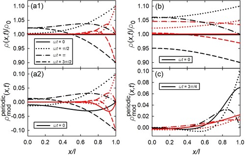
Figure 3(b) compares the cases of negligible reaction-limitation ($L={10}^3$), i.e. entirely diffusion limitation, and both reaction- and diffusion-limitation (L = 1) for M = 2, which corresponds to a lower frequency compared to figure part a. For both L = 1 and ${10}^3$, the same values for D and l are assumed, but only κ differs (see caption, Figure 3). For $L={10}^3$ the gradients of $\rho (x,t)/{\rho }_0$ are smaller in comparison to Figure 3(a), since due to the lower frequency the system can better follow the modulation. For the case of both of reaction- and diffusion-limitation (L = 1, red curves), the spatial shape of the profiles are similar to that for $L={10}^3$ (black curves), however, the absolute values of the modulation of $\rho (x,t)$ are reduced. This is caused by the fact, that due to the reaction-limitation the modulation of the concentration $\rho (x=l,t)$ inside the sample surface is reduced with respect to the modulation at the boundary. This influence of the reaction-limitation, characterised by κ, can be discerned when we combine the relations for L (plate: $\mathrm{\kappa l}/D$, Equation (25(25) $L=\frac{\mathrm{\kappa l}}{D},$(25) )) and M (plate: $\sqrt{2l^2\omega /D}$, Equation (30(30) $M=\sqrt{\frac{2l^2\omega }{D}},$(30) )) yielding (54) $\frac{\kappa }{l}=\frac{2L}{M^2}\omega .$(54) With M = 2, one obtains $\kappa /l=500\omega$ for $L={10}^3$ and $0.5\omega$ for L = 1. For L = 1, the reaction rate $\kappa /l$ is in the range of the modulation frequency ω, meaning that within the modulation time the concentration $\rho (x=l,t)$ inside the sample surface cannot attain the concentration imposed by the modulation. For high values of L the reaction rate is high with respect to ω, therefore, plays no role and $\rho (x=l,t)$ reaches the imposed modulation amplitude. This limit of negligible reaction-limitation ($L={10}^3$), i.e. entirely diffusion limitation, corresponds to the boundary condition according to Equation (16(16) $\rho (x=l,t)={\rho }_0+\hat{\rho }\sin \left(\mathrm{\omega t}\right)$(16) ) as schematically visualised in Figure 1(c), compared to the general case of both diffusion- and reaction-limitation in Figure 1(b).

The spatial variation ${\rho }_{\mathrm{mod}}^{\mathrm{periodic}}(x,t)$ in the high-frequency regime shown in Figure 3(c) nicely reflects the different limiting phase shifts of $-\pi /4$ ($L={10}^3$) and $-\pi /2$ (L = 1). The amount of loaded species corresponds to the net area under the respective ${\rho }_{\mathrm{mod}}^{\mathrm{periodic}}-x$ curve. For the entirely diffusion-limited case ($L={10}^3$), this area maximum is reached approximately for $\mathrm{\omega t}=3\pi /4$, as can be seen by a comparison of the $\pi /2$- and $3\pi /4$-curves. This means a shift by $-\pi /4$ with respect to the sinusoidal maximum at the surface at $\mathrm{\omega t}=\pi /2$. For the diffusion- and reaction-limited case (L = 1), this area maximum is not yet obtained for $\mathrm{\omega t}=3\pi /4$ due to the additional retardation by reaction, but only approximately for $\mathrm{\omega t}=\pi$, corresponding to a phase shift $-\pi /2$. Different M-values of 5 and 10 for L = 1 and ${10}^3$, respectively, had to used here in order to visualise in each case a state in the high-frequency regime, but with still noticeable amplitude (compare Figure 2(a,b)).

3.5. Impedance

The particle transport behaviour can be studied by measuring the electrical current associated with electrode reaction, Equation (1(1) ${\mathrm{H}}^{+}+{\mathrm{e}}^{-}+\mathrm{i}\leftrightarrows \mathrm{H}.$(1) ). We restrict the following consideration to the oscillating part of the particle current density, Equation (29(29) $\begin{array}{rl}{j}_{\mathrm{s}}& =\sum _{n=1}^{\mathrm{\infty }}\frac{2\mathrm{L\kappa }}{({\overline{\text{β}}}_n^2+L^2+L)}[{\rho }_0^{\mathrm{ini}}-{\rho }_0+\frac{1}{2}\hat{\rho }\frac{M^2{\overline{\text{β}}}_n^2}{{\overline{\text{β}}}_n^4+\frac{1}{4}{M}^4}]\exp (-\frac{D{\overline{\text{β}}}_n^2}{l^2}t)\\ & -2l\hat{\rho }\frac{\mathrm{L\omega }}{M}\frac{C}{\sqrt{A^2+B^2}}\sin (\mathrm{\omega t}+{\varphi }_0+\frac{\pi }{2}),\end{array}$(29) ), i.e. when the time-exponentially decaying transient part has faded away. The oscillating part of the electrical current density for planar electrode, Equation (29(29) $\begin{array}{rl}{j}_{\mathrm{s}}& =\sum _{n=1}^{\mathrm{\infty }}\frac{2\mathrm{L\kappa }}{({\overline{\text{β}}}_n^2+L^2+L)}[{\rho }_0^{\mathrm{ini}}-{\rho }_0+\frac{1}{2}\hat{\rho }\frac{M^2{\overline{\text{β}}}_n^2}{{\overline{\text{β}}}_n^4+\frac{1}{4}{M}^4}]\exp (-\frac{D{\overline{\text{β}}}_n^2}{l^2}t)\\ & -2l\hat{\rho }\frac{\mathrm{L\omega }}{M}\frac{C}{\sqrt{A^2+B^2}}\sin (\mathrm{\omega t}+{\varphi }_0+\frac{\pi }{2}),\end{array}$(29) ), reads with A, B, C according to Equation (33(33) $\begin{array}{rl}A& =L(\sin M-\sinh M)+M(\cos M-\cosh M),\\ B& =L(\sin M+\sinh M),\\ C& =\cosh M-\cos M.\end{array}$(33) ): (55) $j_{\mathrm{s},\mathrm{mod}}=-e\hat{\rho }\frac{2\mathrm{lL\omega }}{M}\frac{C}{\sqrt{A^2+B^2}}\sin (\mathrm{\omega t}+{\varphi }_0+\frac{\pi }{2}),$(55) with e the elementary charge,³ corresponding to the valency z = 1 for protons.

In general, the relation between the oscillating input voltage $U=\hat{U}\sin \left(\mathrm{\omega t}\right)$, Equation (2(2) $U\left(t\right)=U_0+\hat{U}\sin \left(\mathrm{\omega t}\right),$(2) ), and the resulting oscillating output current density is characterised by a transfer function that describes the frequency response of the system. This transfer function corresponds to the admittance (56) $Y\left(\omega \right)=\frac{I_0}{U_0}\exp \left(i{\varphi }_Z\right),$(56) where $U_0$ and $I_0$ are the current and voltage amplitude, respectively, and ${\varphi }_Z$ the phase between voltage and current [22,23]. As the admittance $Y\left(\omega \right)$ is the inverse of the impedance $Z\left(\omega \right)$, one obtains: (57) $Z\left(\omega \right)=\frac{1}{Y\left(\omega \right)}=\frac{U_0}{I_0}\exp (-i{\varphi }_Z).$(57) For the special case of our model (58) $I_0=e\hat{\rho }\frac{2\mathrm{lL\omega }}{M}\frac{C}{\sqrt{A^2+B^2}},$(58) $U_0=\hat{U}$ and ${\varphi }_Z={\varphi }_0+\pi /2$ (for $U_0$ see Equation (2(2) $U\left(t\right)=U_0+\hat{U}\sin \left(\mathrm{\omega t}\right),$(2) ), for $I_0$ and ${\varphi }_Z$ Equation (55(55) $j_{\mathrm{s},\mathrm{mod}}=-e\hat{\rho }\frac{2\mathrm{lL\omega }}{M}\frac{C}{\sqrt{A^2+B^2}}\sin (\mathrm{\omega t}+{\varphi }_0+\frac{\pi }{2}),$(55) )). The faradaic impedance $Z_{\mathrm{f}}\left(\omega \right)$ calculated according to our model is therefore as follows: (59) $Z_{\mathrm{f}}\left(\omega \right)=\frac{\hat{U}}{e\hat{\rho }}\frac{M}{2\mathrm{lL\omega }}\frac{\sqrt{A^2+B^2}}{C}\exp (-i{\varphi }_Z).$(59) Figure 4 shows the real (Re$\left(Z_{\mathrm{f}}\right)$) and imaginary part (Im$\left(Z_{\mathrm{f}}\right)$) of the complex impedance in the Nyquist-plot presentation. The associated impedance parameters for the frequency limits $\omega =0$ and $\omega \to \mathrm{\infty }$ are summarised in Table 1. The table shows for both frequency limits, the parameters for the general case of diffusion and reaction limitation, for the special case of entirely reaction limitation ($L\to 0$) given in the limit of high diffusivity ($D\to \mathrm{\infty }$) and, for the special case of entirely diffusion limitation ($L\to \mathrm{\infty }$) given in the limit of high reaction rates ($\kappa \to \mathrm{\infty }$).

Figure 4. Real (Re$\left(Z_{\mathrm{f}}\right)/\left(\hat{U}/\right(e\hat{\rho }\left)\right)$) and negative imaginary part (−Im$\left(Z_{\mathrm{f}}\right)/\left(\hat{U}/\right(e\hat{\rho }\left)\right)$) of complex impedance, Equation (59(59) $Z_{\mathrm{f}}\left(\omega \right)=\frac{\hat{U}}{e\hat{\rho }}\frac{M}{2\mathrm{lL\omega }}\frac{\sqrt{A^2+B^2}}{C}\exp (-i{\varphi }_Z).$(59) ), of planar electrode in Nyquist-plot presentation for various values of L, Equation (25(25) $L=\frac{\mathrm{\kappa l}}{D},$(25) ). The intersection with the real axis, i.e. −Im$\left(Z_{\mathrm{f}}\right)/\left(\hat{U}/\right(e\hat{\rho }\left)\right)$, marks the limit $\omega \to \mathrm{\infty }$, whereas −Im$\left(Z_{\mathrm{f}}\right)/\left(\hat{U}/\right(e\hat{\rho }\left)\right)\to -\mathrm{\infty }$ marks the limit $\omega =0$. For easy visualising, simple values in power of tens are used for the parameters, D (unit: m${}^2$/s), κ (unit: m/s), and l (unit: m). Variation of κ with D = 1 and l = 1: κ = 1 (L = 1, black solid), 10 (L = 10, blue dashed), ${10}^3$ ($L={10}^3$, blue dashed-dotted); variation of D with $\kappa =1$ and l = 1: D = 1 (L = 1, black solid), 10 (L = 0.1, black dashed), ${10}^3$ ($L={10}^{-3}$, black dashed-dotted). Relations for the $Z_{\mathrm{f}}$-values at the frequency limits $\omega =0$ and $\omega \to \mathrm{\infty }$ are given in Table 1.

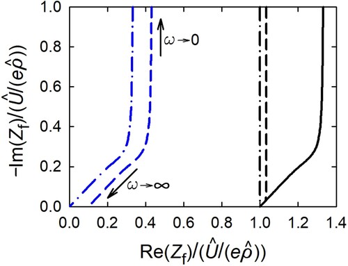
Table 1. Amplitude $Z(=U_0/I_0)$, real part of amplitude Re$\left(Z_{\mathrm{f}}\right)$ and phase ${\varphi }_Z$ of the complex impedance, Equation (59(59) $Z_{\mathrm{f}}\left(\omega \right)=\frac{\hat{U}}{e\hat{\rho }}\frac{M}{2\mathrm{lL\omega }}\frac{\sqrt{A^2+B^2}}{C}\exp (-i{\varphi }_Z).$(59) ), and of the phase ${\varphi }_0$, Equation (32(32) ${\varphi }_0=\arctan \frac{A}{B}+0\text{or}\pi$(32) ), for $\omega =0$ and $\omega \to \mathrm{\infty }$ in the general case of diffusion and reaction limitation as well as in the special case of either reaction or diffusion limitation. Planar electrode; L, M according to Equations (25(25) $L=\frac{\mathrm{\kappa l}}{D},$(25) ) and (30(30) $M=\sqrt{\frac{2l^2\omega }{D}},$(30) ), respectively.

	$\omega =0$ (M = 0)			$\omega \to \mathrm{\infty }$ ($M\to \mathrm{\infty }$)
limitation	Diffusion and reaction	Reaction	Diffusion	Diffusion and reaction	Reaction	Diffusion ${}^{\left(\mathrm{a}\right)}$
		$L\to 0$	$L\to \mathrm{\infty }$		$L\to 0$	$L\to \mathrm{\infty }$
		$D\to \mathrm{\infty }$	$\kappa \to \mathrm{\infty }$		$D\to \mathrm{\infty }$	$\kappa \to \mathrm{\infty }$
${\varphi }_0$	0	0	0	$-\pi /2$	$-\pi /2$	$-\pi /4$
${\varphi }_Z$	$\pi /2$	$\pi /2$	$\pi /2$	0	0	$\pi /4$
$Z/\left(\hat{U}/\right(e\hat{\rho }\left)\right)$)	$1/\left(\mathrm{l\omega }\right)$	$1/\left(\mathrm{l\omega }\right)$	$1/\left(\mathrm{l\omega }\right)$	$1/\kappa$	$1/\kappa$	$1/\sqrt{\mathrm{\omega D}}$
Re$\left(Z_{\mathrm{f}}\right)/\left(\hat{U}/\right(e\hat{\rho }\left)\right)$	$(1+L/3)/\kappa$	1/κ	$l/\left(3D\right)$	$1/\kappa$	$1/\kappa$	$1/\sqrt{2\mathrm{\omega D}}$

${}^{\left(\mathrm{a}\right)}$ valid for $M/L=\sqrt{2\mathrm{\omega D}/\kappa }\ll 1$.

The Nyquist-plot, Figure 4, shows the typical Warburg-impedance behaviour [22–24] with the slope $\pi /4$ of the Im$\left(Z_{\mathrm{f}}\right)$-Re$\left(Z_{\mathrm{f}}\right)$-curve for large ω. The intersection of the curve with the real axis in the limit $\omega \to \mathrm{\infty }$, which is denoted the interfacial transfer resistance $R_{\mathrm{t}}$ in the theory of electrochemical impedance spectroscopy (EIS) [10], is given by $\hat{U}/\left(e\hat{\rho }\right)\times 1/\kappa$ and tends to zero for high reaction rates κ. In the limit $\omega =0$, the real part becomes $\hat{U}/\left(e\hat{\rho }\right)\times (1+L/3)1/\kappa$, which corresponds $R_{\mathrm{t}}+1/3R_{\mathrm{d}}$ [10], with the so-called diffusion resistance $R_{\mathrm{d}}=\hat{U}/\left(e\hat{\rho }\right)\times l/D$ (with $L/\kappa =l/D$), which tends to zero for high diffusivities. In the reaction-controlled limit, the Im$\left(Z_{\mathrm{f}}\right)$-Re$\left(Z_{\mathrm{f}}\right)$-curve is a vertical line with the real part Re$\left(Z_{\mathrm{f}}\right)=\hat{U}/\left(e\hat{\rho }\right)\times 1/\kappa$.

With the interfacial transfer resistance $R_{\mathrm{t}}$ and diffusion resistance $R_{\mathrm{d}}$ defined above, one can interpret the parameter $L=\mathrm{\kappa l}/D$, Equation (25(25) $L=\frac{\mathrm{\kappa l}}{D},$(25) ), as the resistance ratio (60) $L=\frac{R_{\mathrm{d}}}{R_{\mathrm{t}}}.$(60) $R_{\mathrm{d}}>R_{\mathrm{t}}$ or $R_{\mathrm{d}}<R_{\mathrm{t}}$ defines the regime of diffusion- or reaction limitation, respectively, in line what has been discussed in Section 3.2.

For negligible transfer resistance, i.e. in the entirely diffusion-limited regime, the faradaic impedance, Equation (59(59) $Z_{\mathrm{f}}\left(\omega \right)=\frac{\hat{U}}{e\hat{\rho }}\frac{M}{2\mathrm{lL\omega }}\frac{\sqrt{A^2+B^2}}{C}\exp (-i{\varphi }_Z).$(59) ), reads: (61) $Z_{\mathrm{f}}\left(\omega \right)=\frac{\hat{U}}{e\hat{\rho }}\frac{l}{D}\frac{\sqrt{2({\sinh }^{2}M+{\sin }^{2}M)}}{M(\cosh M-\cos M)}\exp (-i{\varphi }_Z)$(61) with ${\varphi }_Z={\varphi }_0+\pi /2$ and ${\varphi }_0$ according to Equation (48(48) ${\varphi }_0=\arctan \frac{\sin M-\sinh M}{\sin M+\sinh M}$(48) ).

3.6. Comparison of modulation with literature and application potentials beyond

The overall focus of this work is on the effect of an sinusoidal modulation of the surface particle concentration and the associated variation of particle insertion on the temporal and spatial change of bulk concentration in the electrode. This is a very general bulk diffusion problem that occurs, e.g. when charging materials with particles, like hydrogen or lithium, by electrochemical means, as treated in this work, or from the gas phase.

We start the discussion by comparing our work with the research area that comes closest to our model, namely hydrogen absorption and diffusion in electrodes studied by electrochemical impedance spectroscopy (e.g. Refs. [10, 15, 25–30]). In the well-established EIS-models, the hydrogen insertion mechanism is assumed to be either a two step process, including hydrogen adsorption and subsequent absorption, or to be directly absorbed in a one step process [24]. In EIS measurements, an electrochemical system in equilibrium or in steady state is perturbed by applying a sinusoidal signal, e.g. a voltage, over a wide frequency range and monitoring the sinusoidal response, e.g. a current, of this perturbed system [23]. For the special case of hydrogen insertion, the sinusoidal electrode current response by an oscillating voltage is affected, on the one hand, by hydrogen reactions at the electrode-electrolyte interface, like hydrogen ad- and absorption or hydrogen gas evolution at the electrode surface, and, on the other hand, by the subsequent hydrogen diffusion in the bulk. The resulting electrode current is usually calculated by adding the current contributions of these individual steps, which means that the diffusion equation is solved independently from the hydrogen reactions at the surface [10, 24].

In this work, we used a different approach to model hydrogen absorption and diffusion in electrodes, as compared to existing theories based on electrochemical impedance spectroscopy. The attractiveness of our model lies in the way how the particle current density $j_{\mathrm{s}}\left(t\right)$, Equation (29(29) $\begin{array}{rl}{j}_{\mathrm{s}}& =\sum _{n=1}^{\mathrm{\infty }}\frac{2\mathrm{L\kappa }}{({\overline{\text{β}}}_n^2+L^2+L)}[{\rho }_0^{\mathrm{ini}}-{\rho }_0+\frac{1}{2}\hat{\rho }\frac{M^2{\overline{\text{β}}}_n^2}{{\overline{\text{β}}}_n^4+\frac{1}{4}{M}^4}]\exp (-\frac{D{\overline{\text{β}}}_n^2}{l^2}t)\\ & -2l\hat{\rho }\frac{\mathrm{L\omega }}{M}\frac{C}{\sqrt{A^2+B^2}}\sin (\mathrm{\omega t}+{\varphi }_0+\frac{\pi }{2}),\end{array}$(29) ), is calculated. This particle current density through the electrode-electrolyte interface is obtained directly by solving the diffusion equation (Equation (17(17) $\frac{\mathrm{\partial }\rho }{\mathrm{\partial }t}=D\frac{{\mathrm{\partial }}^2\rho }{\mathrm{\partial }{x}^2}.$(17) )) with a boundary condition, Equation (19(19) ${D\frac{\mathrm{\partial }\rho }{\mathrm{\partial }x}|}_{x=l}=\kappa ({\rho }_0+\hat{\rho }\sin (\mathrm{\omega t})-\rho (l\left)\right).$(19) ), which includes, on the one hand, the modulation and, on the other hand, the reaction rate of particle insertion. The thereby derived current density $j_{\mathrm{s}}\left(t\right)$ catches not only the modulation behaviour in a stationary state, as it is the case in the published EIS-models, but also the transient behaviour. A transient behaviour arises, on the one hand, since the initial condition is not restricted to the mean value about which is modulated. On the other hand, starting the modulation at the time t = 0 also gives rise to a transient (see additional summand, Equation (A7(A7) $\frac{1}{2}\hat{\rho }\frac{M^2{\overline{\text{β}}}_n^2}{{\overline{\text{β}}}_n^4+\frac{1}{4}{M}^4}$(A7) ), in Equation (29(29) $\begin{array}{rl}{j}_{\mathrm{s}}& =\sum _{n=1}^{\mathrm{\infty }}\frac{2\mathrm{L\kappa }}{({\overline{\text{β}}}_n^2+L^2+L)}[{\rho }_0^{\mathrm{ini}}-{\rho }_0+\frac{1}{2}\hat{\rho }\frac{M^2{\overline{\text{β}}}_n^2}{{\overline{\text{β}}}_n^4+\frac{1}{4}{M}^4}]\exp (-\frac{D{\overline{\text{β}}}_n^2}{l^2}t)\\ & -2l\hat{\rho }\frac{\mathrm{L\omega }}{M}\frac{C}{\sqrt{A^2+B^2}}\sin (\mathrm{\omega t}+{\varphi }_0+\frac{\pi }{2}),\end{array}$(29) )). Such transient behaviour for modulation has for instance been treated for heat conduction [31]. One should note that the present model considers exclusively the direct hydrogen absorption, but not hydrogen gas evolution as competitive reaction at the electrode surface.

Since in this work the used boundary condition for solving the diffusion equation includes also the reaction rate (as stated above), the derived faradaic impedance $Z_{\mathrm{f}}$ from the current density $j_{\mathrm{s}}\left(t\right)$ intrinsically contains both the interfacial transfer resistance $R_{\mathrm{t}}$ and the diffusion impedance $Z_{\mathrm{d}}$ (see Section 3.5). For the calculation of $Z_{\mathrm{f}}$ the full solution's transient part, which is time-exponentially decaying, was neglected. It can be shown that the faradaic impedance given by Montella et al. (Equation (28) in Ref. [10]) agrees with the present solution, Equation (59(59) $Z_{\mathrm{f}}\left(\omega \right)=\frac{\hat{U}}{e\hat{\rho }}\frac{M}{2\mathrm{lL\omega }}\frac{\sqrt{A^2+B^2}}{C}\exp (-i{\varphi }_Z).$(59) ), taking into account that the parameter L characterises the ratio of diffusion and transfer resistance, Equation (60(60) $L=\frac{R_{\mathrm{d}}}{R_{\mathrm{t}}}.$(60) ).⁴ On the other side, with respect to impedance, the present model exclusively addresses the faradaic part, which is caused by particle flux through the interface. As already mentioned, the additional faradaic contribution due to the hydrogen evolution reaction at the electrode's surface is also not considered here. Furthermore the charging part of the electrode-electrolyte interface associated with double layer capacitance is not taken into account, which explains the absence of a high-frequency arc in the calculated impedance spectra in Figure 4 as compared to literature [10, 26]. Charging effects of the electrode's surface on the bulk diffusion process of the inserted particles, i.e. ions, can be neglected, as in metals the width of the evolving space charge region next to the electrode-electrolyte interface is restricted to only 1 Å [32] due to their high charge carrier density.

Besides the general case of diffusion and reaction affected particle insertion, various groups focused on entirely diffusion-limited particle transport in electrodes (e.g. Ref. [33–36]). The diffusion–reaction model in the present work also contains the expressions for the phase angle, Equations (48(48) ${\varphi }_0=\arctan \frac{\sin M-\sinh M}{\sin M+\sinh M}$(48) ) and (49(49) ${\varphi }_0=\arctan \frac{-J_1^{\mathrm{Im}}(J_0^{\mathrm{Re}}-J_0^{\mathrm{Im}})+J_1^{\mathrm{Re}}(J_0^{\mathrm{Re}}+J_0^{\mathrm{Im}})}{J_1^{\mathrm{Re}}(J_0^{\mathrm{Re}}-J_0^{\mathrm{Im}})+J_1^{\mathrm{Im}}(J_0^{\mathrm{Re}}+J_0^{\mathrm{Im}})}.$(49) ), and the amplitude, Equations (50(50) $\hat{n}=\sqrt{2}\frac{\hat{\rho }}{{\rho }_0}\frac{1}{M}\frac{\cosh M-\cos M}{\sqrt{{\sin }^{2}M+{\sinh }^{2}M}}$(50) ) and (51(51) $\hat{n}=2\frac{\hat{\rho }}{{\rho }_0}\frac{1}{M}\frac{\sqrt{2\left(\right(J_1^{\mathrm{Re}}{)}^2+\left(J_1^{\mathrm{Im}}{)}^2\right)}}{\sqrt{\left(\right(J_0^{\mathrm{Re}}{)}^2+\left(J_0^{\mathrm{Im}}{)}^2\right)}}.$(51) ), in the limiting case of entirely diffusion-limitation ($L\to \mathrm{\infty }$). In this limit, the same faradaic impedance, Equation (61(61) $Z_{\mathrm{f}}\left(\omega \right)=\frac{\hat{U}}{e\hat{\rho }}\frac{l}{D}\frac{\sqrt{2({\sinh }^{2}M+{\sin }^{2}M)}}{M(\cosh M-\cos M)}\exp (-i{\varphi }_Z)$(61) ), is obtained as reported earlier (Equation (25) in Ref. [35], Equation (24) in Ref. [36]); the same is true for the modulated density function ${\rho }_{\mathrm{mod}}^{\mathrm{periodic}}$ in this limit, Equation (52(52) ${\rho }_{\mathrm{mod}}^{\mathrm{periodic}}(x,t)=\hat{\rho }\sqrt{\frac{\cos \left(2\mathrm{mx}\right)+\cosh \left(2\mathrm{mx}\right)}{\cos M+\cosh M}}\sin (\mathrm{\omega t}+{\varphi }_0)$(52) ), which agrees with the results reported by Ding and Petuskey (Equation (28) in Ref. [34]).

The calculated faradaic impedance spectra given in Figure 4 are not only in good accordance with theoretical models, but agree also very well with experimental data (see, e.g. Refs. [37–39]). In potential regions where hydrogen evolution plays no dominant role, the electrochemical impedance spectra recorded by Gabrielli et al. (Figure (2) in Ref. [37]), Yang and Pyun (Figure (2) in Ref. [38]) and Losiewicz and Lasia (Figure (8b) in Ref. [39]) are in good accordance with the general case of diffusion and reaction affected hydrogen insertion, modeled in this work. The measured spectra show the typical Warburg-impedance behaviour in the middle frequency range, visible by the slope $\pi /4$ of the Im($Z_{\mathrm{f}}$)-Re($Z_{\mathrm{f}}$)-curve, and the purely capacitive line at very low frequencies and have therefore in the middle- and low-frequency range a similar shape as the calculated spectra presented in Figure 4. The high-frequency arc in the measured impedance spectra in the literature is caused by the double layer capacitance associated with electrode-electrolyte interface charging, which is parallel connected to the interfacial transfer resistance $R_{\mathrm{t}}$. This high-frequency arc is missing in the calculated faradaic impdeance spectra (see Figure 4) due to the neglect of this interfacial charging, as mentioned above. The shift of the impedance spectrum on the Re($Z_{\mathrm{f}}$)-axis of the calculated spectra presented in Figure 4 is, however, caused by the interfacial transfer resistance $R_{\mathrm{t}}$, which is also in good accordance with the literature.

Furthermore, it is worthwhile to mention that the general solution of $j_{\mathrm{s}}$, Equation (29(29) $\begin{array}{rl}{j}_{\mathrm{s}}& =\sum _{n=1}^{\mathrm{\infty }}\frac{2\mathrm{L\kappa }}{({\overline{\text{β}}}_n^2+L^2+L)}[{\rho }_0^{\mathrm{ini}}-{\rho }_0+\frac{1}{2}\hat{\rho }\frac{M^2{\overline{\text{β}}}_n^2}{{\overline{\text{β}}}_n^4+\frac{1}{4}{M}^4}]\exp (-\frac{D{\overline{\text{β}}}_n^2}{l^2}t)\\ & -2l\hat{\rho }\frac{\mathrm{L\omega }}{M}\frac{C}{\sqrt{A^2+B^2}}\sin (\mathrm{\omega t}+{\varphi }_0+\frac{\pi }{2}),\end{array}$(29) ), contains as special case the loading/unloading without modulation ($\hat{\rho }=0$ in Equation (29(29) $\begin{array}{rl}{j}_{\mathrm{s}}& =\sum _{n=1}^{\mathrm{\infty }}\frac{2\mathrm{L\kappa }}{({\overline{\text{β}}}_n^2+L^2+L)}[{\rho }_0^{\mathrm{ini}}-{\rho }_0+\frac{1}{2}\hat{\rho }\frac{M^2{\overline{\text{β}}}_n^2}{{\overline{\text{β}}}_n^4+\frac{1}{4}{M}^4}]\exp (-\frac{D{\overline{\text{β}}}_n^2}{l^2}t)\\ & -2l\hat{\rho }\frac{\mathrm{L\omega }}{M}\frac{C}{\sqrt{A^2+B^2}}\sin (\mathrm{\omega t}+{\varphi }_0+\frac{\pi }{2}),\end{array}$(29) )) which electrochemically is monitored by the potential step method. In fact, this particular textbook solution corresponds to that quoted by Montella et al. (Equation (28) in Ref. [10]) and Pyun et al. (Equation (19) in Ref. [2]). Therefore, our more comprehensive model for direct hydrogen absorption bridges the gap between EIS and the potential step method.

Related to electrochemical methods, we find similarities of our model also to other research topics where modulated diffusion processes are considered. Electrochemical impedance spectroscopy of electrolyte-filled porous electrodes of cylindrical shape reveals a similar impedance response as shown in Figure 4 (see, e.g. Figure 2(a) in Ref. [40]). In this context, the phase shift given in Equation (45(45) ${\varphi }_0=\arctan \frac{L[-J_1^{\mathrm{Im}}(J_0^{\mathrm{Re}}-J_0^{\mathrm{Im}})+J_1^{\mathrm{Re}}(J_0^{\mathrm{Re}}+J_0^{\mathrm{Im}}\left)\right]-M\left(\right(J_1^{\mathrm{Re}}{)}^2+\left(J_1^{\mathrm{Im}}{)}^2\right)}{L\left[J_1^{\mathrm{Re}}\right(J_0^{\mathrm{Re}}-J_0^{\mathrm{Im}})+J_1^{\mathrm{Im}}(J_0^{\mathrm{Re}}+J_0^{\mathrm{Im}}\left)\right]}+0\text{or}\pi$(45) ) and shown in Figure 2 corresponds to the scenario of radial diffusion within the electrolyte in a cylindrical pore, as treated by de Levie (Figure 5 in Ref. [41]).

Another field of modulation – not related to electrochemical methods – pertains to permeation of hydrogen through metallic membranes driven by different gas pressures on both sides of the membrane [42–44]. Upon slight modulation of the pressure on the entrance side with elevated pressure, a modulation of the lower pressure on the down-stream side of the membrane is imposed with a characteristic phase shift. This phase shift enables conclusions on the rate-limiting processes (diffusion, permeation or surface processes). Modelling and measurements are restricted to quasi-steady state, so that the transient behaviour is not captured. Such kind of studies by gas pressure modulation might be extended also to loading (instead of permeation) by making use of the model outlined in the present work.

The present model appears also highly suitable for studying modulated loading by measuring changes of the bulk properties of the sample as, e.g. by dilatometry. As shown in detail in Figure 3, a modulation of the surface concentration leads to a significant change in the bulk concentration profile of the diffusing particles. As these concentration changes cause the electrode to expand or contract, also length change measurements by dilatometry [45] appear attractive for studying modulated hydrogen loading. This would expand the application potentials of modulated dilatometry which so far mainly focused on temperature modulation (see Ref. [4] and references therein). Dilatometry upon electrochemical loading offers the advantage that it may grasp all three of the aforementioned types of voltage-induced concentration variations $n\left(t\right)$, Equation (28(28) $\begin{array}{rl}n\left(t\right)& =1-\sum _{n=1}^{\mathrm{\infty }}\frac{2L^2}{{\overline{\text{β}}}_n^2({\overline{\text{β}}}_n^2+L^2+L)}[\frac{{\rho }_0-{\rho }_0^{\mathrm{ini}}}{{\rho }_0}-\frac{1}{2}\frac{\hat{\rho }}{{\rho }_0}\frac{M^2{\overline{\text{β}}}_n^2}{{\overline{\text{β}}}_n^4+\frac{1}{4}{M}^4}]\exp (-\frac{D{\overline{\text{β}}}_n^2}{l^2}t)\\ & +2\frac{\hat{\rho }}{{\rho }_0}\frac{L}{M}\frac{C}{\sqrt{A^2+B^2}}\sin (\mathrm{\omega t}+{\varphi }_0)\end{array}$(28) ), in one measuring run, i.e. the transient part associated with an initial step-like variation of the voltage, the transient part upon starting the oscillation, and the periodic part with the modulation in the quasi-stationary state. By means of the model, specific information on the kinetics could be derived from the phase shift between modulation voltage and the length change as outlined in Subsection 3.3.

As mentioned at the beginning (Section 2.1.1) already, trapping and detrapping of hydrogen at defects inside the electrode is – so far – not taken into account in our modulation model. Diffusion and trapping were initially treated, e.g. by McNabb and Foster [46] or Oriani [47], although without modulation. With modulation, this more complex scenario of additional hydrogen trapping within the electrode is considered in some of the aformentioned studies by electrochemical methods (e.g. [2, 24, 35]) or by gas permeation [43, 44]. The focus in these various studies is on integral characteristic quantities (current, impedance, permeation) rather than on the spatial evolution of the diffusing species inside the sample upon loading. An example for taking into account trapping and detrapping in the diffusion–reaction model has been given in our recent publication on the mean time of loading without modulation [20]. In this context, it is worthwhile to add that diffusion–reaction models similar to those presented here are successfully applied, although without modulation, in the field of positron annihilation studies of defects, namely to describe the diffusion- and reaction controlled trapping of positrons at extended lattice defects, such as grain boundaries or matrix-precipitate interfaces [48, 49].

4. Conclusion

In conclusion, the present work treats the bulk-diffusion problem of electrochemically inserted particles (e.g. hydrogen) in planar or cylindrical electrodes with a boundary condition, which considers on the one hand a sinusoidal oscillation of the particle flux and on the other hand the reaction rate of particle insertion into the electrode. The solution of this so-called diffusion–reaction model with superimposed modulation gives the particle (e.g. hydrogen) concentration within the sample (see Section 2.3, especially Equation (34(34) $\rho (x,t)={\rho }_{\mathrm{unmod}}(x,t)+{\rho }_{\mathrm{mod}}^{\mathrm{transient}}(x,t)+{\rho }_{\mathrm{mod}}^{\mathrm{periodic}}(x,t),$(34) )). The most important key points and results can be summarised as follows:

• The boundary condition, given in Equation (14(14) ${D\frac{\mathrm{\partial }\rho (x,t)}{\mathrm{\partial }x}|}_{x=l}=\kappa \left({\rho }_{\mathrm{eq}}\right(t)-\rho (l,t\left)\right),$(14) ), is derived via the Butler-Volmer equation by using the correlation between the chemical potential, particle concentration and applied potential (see Subsections 2.1.2 and 2.2).

• The used boundary condition leads to a current density $j_{\mathrm{s}}\left(t\right)$, Equation (29(29) $\begin{array}{rl}{j}_{\mathrm{s}}& =\sum _{n=1}^{\mathrm{\infty }}\frac{2\mathrm{L\kappa }}{({\overline{\text{β}}}_n^2+L^2+L)}[{\rho }_0^{\mathrm{ini}}-{\rho }_0+\frac{1}{2}\hat{\rho }\frac{M^2{\overline{\text{β}}}_n^2}{{\overline{\text{β}}}_n^4+\frac{1}{4}{M}^4}]\exp (-\frac{D{\overline{\text{β}}}_n^2}{l^2}t)\\ & -2l\hat{\rho }\frac{\mathrm{L\omega }}{M}\frac{C}{\sqrt{A^2+B^2}}\sin (\mathrm{\omega t}+{\varphi }_0+\frac{\pi }{2}),\end{array}$(29) ), which catches not only the modulation behaviour in a stationary state but also the transient behaviour, which originates in the present work from two different effects. On the one hand, the transient behaviour results from the initial condition, since it is not restricted to the mean value about which is modulated, Equation (A3(A3) ${\rho }_{\mathrm{unmod}}(x,t)={\rho }_0[1-\frac{{\rho }_0-{\rho }_0^{\mathrm{ini}}}{{\rho }_0}\sum _{n=1}^{\mathrm{\infty }}\frac{2\mathrm{Lcos}\left({\overline{\text{β}}}_{n}x/l\right)}{\cos {\overline{\text{β}}}_n({\overline{\text{β}}}_n^2+L^2+L)}\exp (-\frac{D{\overline{\text{β}}}_n^2}{l^2}t)]$(A3) ). On the other hand, starting the modulation at the time t = 0 also gives rise to a transient, Equation (A6(A6) ${\rho }_{\mathrm{mod}}^{\mathrm{transient}}(x,t)=\sum _{n=1}^{\mathrm{\infty }}\frac{1}{2}\hat{\rho }\frac{M^2{\overline{\text{β}}}_n^2}{{\overline{\text{β}}}_n^4+\frac{1}{4}{M}^4}\frac{2\mathrm{Lcos}\left(\overline{\text{β}}x/l\right)}{\cos {\overline{\text{β}}}_n({\overline{\text{β}}}_n^2+L^2+L)}\exp (-\frac{D{\overline{\text{β}}}_n^2}{l^2}t)$(A6) ), which follows only by solving the diffusion equation with an oscillating boundary condition, as done here.

• The observed phase shift between the surface particle concentration modulated by electrochemical means and the bulk particle concentration, shown in Figure 2, provides information whether the particle flux through the electrode–electrolyte interface is influenced more strongly by the insertion reaction or the subsequent diffusion inside the electrode.

• The analysis of the spatial and temporal concentration evolution within the sample Figure 3 yields deeper inside into the loading kinetics then when only the current at the interface is considered.

• When no modulation is considered, the diffusion–reaction model contains as special case for the direct insertion mechanism the electrochemical potential step method.

• By neglecting the transient terms or by waiting long enough until these exponential terms have decayed, the faradaic impedance $Z_{\mathrm{f}}$, Equation (59(59) $Z_{\mathrm{f}}\left(\omega \right)=\frac{\hat{U}}{e\hat{\rho }}\frac{M}{2\mathrm{lL\omega }}\frac{\sqrt{A^2+B^2}}{C}\exp (-i{\varphi }_Z).$(59) ), follows. As the used boundary condition includes also the reaction rate, the derived $Z_{\mathrm{f}}$ from the current density $j_{\mathrm{s}}\left(t\right)$ intrinsically contains both the interfacial transfer resistance $R_{\mathrm{t}}$ and the diffusion impedance $Z_{\mathrm{d}}$ (see Subsection 3.5). The ratio between diffusion and reaction limitation is described via the parameter L, Equations (25(25) $L=\frac{\mathrm{\kappa l}}{D},$(25) ) and (40(40) $L=\frac{\kappa r_0}{D}$(40) ), which characterises the ratio of diffusion and reaction resistance, Equation (60(60) $L=\frac{R_{\mathrm{d}}}{R_{\mathrm{t}}}.$(60) ). The resulting Nyquist plots of $Z_{\mathrm{f}}$ for different limiting cases (e.g. entirely diffusion-controlled) are presented in Figure 4.

It is important to state finally once more that the presented diffusion–reaction model is not only highly suitable to study particle (e.g. hydrogen) insertion in electrodes and subsequent diffusion phenomena in the field of electrochemistry. As outlined at the end of Section 3.6, the model can also be applied

• for other types of loading, e.g. from the gas phase, and

• to other measuring techniques, e.g. dilatometry.

Disclosure statement

No potential conflict of interest was reported by the author(s).

Notes

1 This way of determining $j_{\mathrm{s}}$ is more straightforward than from the boundary condition, Equations (13(13) $j_{\mathrm{s}}\left(t\right)={-D\frac{\mathrm{\partial }\rho (x,t)}{\mathrm{\partial }x}|}_{x=l},$(13) ) and (14(14) ${D\frac{\mathrm{\partial }\rho (x,t)}{\mathrm{\partial }x}|}_{x=l}=\kappa \left({\rho }_{\mathrm{eq}}\right(t)-\rho (l,t\left)\right),$(14) ).

2 Remark: In Ref. [20] κ is denoted α.

3 Note that here the electrical and not the particle current is considered.

4 Remark: $\sqrt{\mathrm{iu}}$ in Equation (28) of Ref. [10] corresponds to $M(1+i)/2$ in the present work, with M according to Equation (30(30) $M=\sqrt{\frac{2l^2\omega }{D}},$(30) ).

Appendix. Details on determination of density function $\rho (x,t)$, $\rho (r,t)$ (cf. Section 2.3)

A.1. Planar electrode

With the Ansatz $\tilde{\rho }=b_1/2\exp \left(\mathrm{\gamma x}\right)+b_2/2\exp (-\mathrm{\gamma x})+b_3$ ($b_i$: arbitrary parameters), the solution of the diffusion equation (22(22) $\frac{{\mathrm{d}}^2\tilde{\rho }}{\mathrm{d}{\mathrm{x}}^2}-{\gamma }^2\tilde{\rho }=-\frac{{\rho }_0^{\mathrm{ini}}}{D}\mathrm{with}{\gamma }^2=\frac{p}{D}.$(22) ) with the boundary condition for x = 0 Equation (20(20) ${\frac{\mathrm{\partial }\rho }{\mathrm{\partial }x}|}_{x=0}=0.$(20) ) reads (A1) $\tilde{\rho }=b_1\cosh \left(\mathrm{\gamma x}\right)+\frac{{\rho }_0^{\mathrm{ini}}}{p}.$(A1) Inserting the oscillating boundary condition, Equation (23(23) ${D\frac{\mathrm{d}\tilde{\rho }}{\mathrm{d}x}|}_{x=l}=\kappa (\frac{{\rho }_0}{p}+\hat{\rho }\frac{\omega }{p^2+{\omega }^2}-\tilde{\rho }(l\left)\right).$(23) ), yields Equation (24(24) $\tilde{\rho }(x,p)=\frac{L({\rho }_0-{\rho }_0^{\mathrm{ini}})\cosh \left(\mathrm{\gamma x}\right)}{p(\mathrm{Lcosh}\text{β}+\text{β}\sinh \text{β})}+\frac{{\rho }_0^{\mathrm{ini}}}{p}+\hat{\rho }\frac{\mathrm{L\omega cosh}\left(\mathrm{\gamma x}\right)}{(p^2+{\omega }^2)(\mathrm{Lcosh}\text{β}+\text{β}\sinh \text{β})},$(24) ).

The inverse of the Laplace transform $\tilde{y}=f\left(p\right)/g\left(p\right)$ according to textbook is given by (Equation 2.59 in Ref. [11]) (A2) $y\left(t\right)=\sum _{r=1}^n\frac{f\left(a_r\right)}{g^{\prime }\left(a_r\right)}\exp \left(a_{r}t\right)$(A2) where $a_r$ denote the roots of $g\left(p\right)$. The retransformation of the unmodulated left and middle part of Equation (24(24) $\tilde{\rho }(x,p)=\frac{L({\rho }_0-{\rho }_0^{\mathrm{ini}})\cosh \left(\mathrm{\gamma x}\right)}{p(\mathrm{Lcosh}\text{β}+\text{β}\sinh \text{β})}+\frac{{\rho }_0^{\mathrm{ini}}}{p}+\hat{\rho }\frac{\mathrm{L\omega cosh}\left(\mathrm{\gamma x}\right)}{(p^2+{\omega }^2)(\mathrm{Lcosh}\text{β}+\text{β}\sinh \text{β})},$(24) ) yields the well-known textbook solution [11]: (A3) ${\rho }_{\mathrm{unmod}}(x,t)={\rho }_0[1-\frac{{\rho }_0-{\rho }_0^{\mathrm{ini}}}{{\rho }_0}\sum _{n=1}^{\mathrm{\infty }}\frac{2\mathrm{Lcos}\left({\overline{\text{β}}}_{n}x/l\right)}{\cos {\overline{\text{β}}}_n({\overline{\text{β}}}_n^2+L^2+L)}\exp (-\frac{D{\overline{\text{β}}}_n^2}{l^2}t)]$(A3) with ${\text{β}}^2=-{\overline{\text{β}}}^2$ ($\text{β}=i\overline{\text{β}}$), with $L=\mathrm{\kappa l}/D$, Equation (25(25) $L=\frac{\mathrm{\kappa l}}{D},$(25) ), and with the roots ${\overline{\text{β}}}_n\tan {\overline{\text{β}}}_n=L$, Equation (31(31) ${\overline{\text{β}}}_n\tan {\overline{\text{β}}}_n=L,$(31) ), which determine ${\overline{\text{β}}}_n$.

For the retransformation of the modulated right part of Equation (24(24) $\tilde{\rho }(x,p)=\frac{L({\rho }_0-{\rho }_0^{\mathrm{ini}})\cosh \left(\mathrm{\gamma x}\right)}{p(\mathrm{Lcosh}\text{β}+\text{β}\sinh \text{β})}+\frac{{\rho }_0^{\mathrm{ini}}}{p}+\hat{\rho }\frac{\mathrm{L\omega cosh}\left(\mathrm{\gamma x}\right)}{(p^2+{\omega }^2)(\mathrm{Lcosh}\text{β}+\text{β}\sinh \text{β})},$(24) ) according to Equation (A2(A2) $y\left(t\right)=\sum _{r=1}^n\frac{f\left(a_r\right)}{g^{\prime }\left(a_r\right)}\exp \left(a_{r}t\right)$(A2) ) the roots (i) $p=\pm \mathrm{i\omega }$ and (ii) $\text{β}\tanh \text{β}=-L$ of the demoninator $(p^2+{\omega }^2)(\mathrm{Lcosh}\text{β}+\text{β}\sinh \text{β})$ have to considered in the following.

A.1.1. Modulation: root (ii), transient part

The derivative of the demoninator of the oscillation part of Equation (24(24) $\tilde{\rho }(x,p)=\frac{L({\rho }_0-{\rho }_0^{\mathrm{ini}})\cosh \left(\mathrm{\gamma x}\right)}{p(\mathrm{Lcosh}\text{β}+\text{β}\sinh \text{β})}+\frac{{\rho }_0^{\mathrm{ini}}}{p}+\hat{\rho }\frac{\mathrm{L\omega cosh}\left(\mathrm{\gamma x}\right)}{(p^2+{\omega }^2)(\mathrm{Lcosh}\text{β}+\text{β}\sinh \text{β})},$(24) ) reads (A4) $g^{\prime }\left(p\right)=(p^2+{\omega }^2)\frac{\mathrm{d}\text{β}}{\mathrm{d}p}\left[\right(L+1)\cosh \text{β}+\text{β}\sinh \text{β}]+2p(\mathrm{Lcosh}\text{β}+\text{β}\sinh \text{β})$(A4) with $\mathrm{d}\text{β}/\mathrm{d}p=l^2/\left(2D\text{β}\right)$. For the root (ii) $\text{β}\tanh \text{β}+L=0$, Equation (A4(A4) $g^{\prime }\left(p\right)=(p^2+{\omega }^2)\frac{\mathrm{d}\text{β}}{\mathrm{d}p}\left[\right(L+1)\cosh \text{β}+\text{β}\sinh \text{β}]+2p(\mathrm{Lcosh}\text{β}+\text{β}\sinh \text{β})$(A4) ) reads with $p=D{\text{β}}^2/l^2=-D{\overline{\text{β}}}^2/l^2$: (A5) $g^{\prime }\left(p\right)=({\overline{\text{β}}}^4+\frac{{\omega }^2{l}^4}{D^2})\frac{D}{2l^2{\overline{\text{β}}}^2}\cos \overline{\text{β}}({\overline{\text{β}}}^2+L^2+L).$(A5) Retransformation according to Equation (A2(A2) $y\left(t\right)=\sum _{r=1}^n\frac{f\left(a_r\right)}{g^{\prime }\left(a_r\right)}\exp \left(a_{r}t\right)$(A2) ) yields for this root the solution: (A6) ${\rho }_{\mathrm{mod}}^{\mathrm{transient}}(x,t)=\sum _{n=1}^{\mathrm{\infty }}\frac{1}{2}\hat{\rho }\frac{M^2{\overline{\text{β}}}_n^2}{{\overline{\text{β}}}_n^4+\frac{1}{4}{M}^4}\frac{2\mathrm{Lcos}\left(\overline{\text{β}}x/l\right)}{\cos {\overline{\text{β}}}_n({\overline{\text{β}}}_n^2+L^2+L)}\exp (-\frac{D{\overline{\text{β}}}_n^2}{l^2}t)$(A6) with $M=(2l^2\omega /D{)}^{1/2}$, Equation (30(30) $M=\sqrt{\frac{2l^2\omega }{D}},$(30) ). Equation (A6(A6) ${\rho }_{\mathrm{mod}}^{\mathrm{transient}}(x,t)=\sum _{n=1}^{\mathrm{\infty }}\frac{1}{2}\hat{\rho }\frac{M^2{\overline{\text{β}}}_n^2}{{\overline{\text{β}}}_n^4+\frac{1}{4}{M}^4}\frac{2\mathrm{Lcos}\left(\overline{\text{β}}x/l\right)}{\cos {\overline{\text{β}}}_n({\overline{\text{β}}}_n^2+L^2+L)}\exp (-\frac{D{\overline{\text{β}}}_n^2}{l^2}t)$(A6) ) represents an additional summand with the coefficient (A7) $\frac{1}{2}\hat{\rho }\frac{M^2{\overline{\text{β}}}_n^2}{{\overline{\text{β}}}_n^4+\frac{1}{4}{M}^4}$(A7) in the series of Equation (A3(A3) ${\rho }_{\mathrm{unmod}}(x,t)={\rho }_0[1-\frac{{\rho }_0-{\rho }_0^{\mathrm{ini}}}{{\rho }_0}\sum _{n=1}^{\mathrm{\infty }}\frac{2\mathrm{Lcos}\left({\overline{\text{β}}}_{n}x/l\right)}{\cos {\overline{\text{β}}}_n({\overline{\text{β}}}_n^2+L^2+L)}\exp (-\frac{D{\overline{\text{β}}}_n^2}{l^2}t)]$(A3) ). It therefore reflects the transient part associated with modulation.

A.1.2. Modulation: root (i), periodic part

For the roots (i) $p=\pm \mathrm{i\omega }$, the demoninator derivative, Equation (A4(A4) $g^{\prime }\left(p\right)=(p^2+{\omega }^2)\frac{\mathrm{d}\text{β}}{\mathrm{d}p}\left[\right(L+1)\cosh \text{β}+\text{β}\sinh \text{β}]+2p(\mathrm{Lcosh}\text{β}+\text{β}\sinh \text{β})$(A4) ), reads (A8) $g^{\prime }\left(p\right)=2p(\mathrm{Lcos}\overline{\text{β}}-\overline{\text{β}}\sin \overline{\text{β}})$(A8) with ${\text{β}}^2=-{\overline{\text{β}}}^2$. For the inverse of the Laplace transform according to Equation (A2(A2) $y\left(t\right)=\sum _{r=1}^n\frac{f\left(a_r\right)}{g^{\prime }\left(a_r\right)}\exp \left(a_{r}t\right)$(A2) ) the solution (A9) ${\rho }_{\mathrm{mod}}^{\mathrm{periodic}}(x,t)=\frac{\hat{\rho }\mathrm{Lcos}\left({\overline{\text{β}}}_{+}x/l\right)\exp \left(\mathrm{i\omega t}\right)}{2i(\mathrm{Lcos}{\overline{\text{β}}}_{+}-{\overline{\text{β}}}_{+}\sin {\overline{\text{β}}}_{+})}-\frac{\hat{\rho }\mathrm{Lcos}\left({\overline{\text{β}}}_{-}x/l\right)\exp (-\mathrm{i\omega t})}{2i(\mathrm{Lcos}{\overline{\text{β}}}_{-}-{\overline{\text{β}}}_{-}\sin {\overline{\text{β}}}_{-})}$(A9) is obtained, where ${\overline{\text{β}}}_{+}$ and ${\overline{\text{β}}}_{-}$ is given by with (A10) ${\overline{\text{β}}}_M=\frac{1}{2}M(1+i),$(A10) with ${\overline{\text{β}}}_M^2=i{M}^2/2={\overline{\text{β}}}_{-}^2=-{\overline{\text{β}}}_{+}^2$.

Integration of Equation (A9(A9) ${\rho }_{\mathrm{mod}}^{\mathrm{periodic}}(x,t)=\frac{\hat{\rho }\mathrm{Lcos}\left({\overline{\text{β}}}_{+}x/l\right)\exp \left(\mathrm{i\omega t}\right)}{2i(\mathrm{Lcos}{\overline{\text{β}}}_{+}-{\overline{\text{β}}}_{+}\sin {\overline{\text{β}}}_{+})}-\frac{\hat{\rho }\mathrm{Lcos}\left({\overline{\text{β}}}_{-}x/l\right)\exp (-\mathrm{i\omega t})}{2i(\mathrm{Lcos}{\overline{\text{β}}}_{-}-{\overline{\text{β}}}_{-}\sin {\overline{\text{β}}}_{-})}$(A9) ) according to Equation (26(26) $n\left(t\right)=\frac{A^{\prime }}{{\rho }_0{A}^{\prime }l}{\int }_0^l\rho (x,t)\mathrm{d}x$(26) ) yields the volume-averaged fraction: (A11) $n_{\mathrm{mod}}^{\mathrm{periodic}}\left(t\right)=\frac{\hat{\rho }}{{\rho }_0}[\frac{\mathrm{Lexp}\left(\mathrm{i\omega t}\right)}{2i{\overline{\text{β}}}_{+}(\mathrm{Lcot}{\overline{\text{β}}}_{+}-{\overline{\text{β}}}_{+})}-\frac{\mathrm{Lexp}(-\mathrm{i\omega t})}{2i{\overline{\text{β}}}_{-}(\mathrm{Lcot}{\overline{\text{β}}}_{-}-{\overline{\text{β}}}_{-})}].$(A11) The complex arguments ${\overline{\text{β}}}_{-}=\frac{1}{2}M(1+i)$, ${\overline{\text{β}}}_{+}=\frac{1}{2}M(-1+i)$ can be eliminated by making use of relations for trigonometric functions with complex argument ($\cot {\overline{\text{β}}}_{-}=-(\sin M-\mathrm{isinh}M)/(\cos M-\cosh M))$ yielding finally the $\sin (\mathrm{\omega t}+{\mathrm{\Phi }}_0)$-term in Equation (28(28) $\begin{array}{rl}n\left(t\right)& =1-\sum _{n=1}^{\mathrm{\infty }}\frac{2L^2}{{\overline{\text{β}}}_n^2({\overline{\text{β}}}_n^2+L^2+L)}[\frac{{\rho }_0-{\rho }_0^{\mathrm{ini}}}{{\rho }_0}-\frac{1}{2}\frac{\hat{\rho }}{{\rho }_0}\frac{M^2{\overline{\text{β}}}_n^2}{{\overline{\text{β}}}_n^4+\frac{1}{4}{M}^4}]\exp (-\frac{D{\overline{\text{β}}}_n^2}{l^2}t)\\ & +2\frac{\hat{\rho }}{{\rho }_0}\frac{L}{M}\frac{C}{\sqrt{A^2+B^2}}\sin (\mathrm{\omega t}+{\varphi }_0)\end{array}$(28) ). In an analogous manner, these complex arguments can be eliminated for ${\rho }_{\mathrm{mod}}^{\mathrm{periodic}}(x,t)$, Equation (A9(A9) ${\rho }_{\mathrm{mod}}^{\mathrm{periodic}}(x,t)=\frac{\hat{\rho }\mathrm{Lcos}\left({\overline{\text{β}}}_{+}x/l\right)\exp \left(\mathrm{i\omega t}\right)}{2i(\mathrm{Lcos}{\overline{\text{β}}}_{+}-{\overline{\text{β}}}_{+}\sin {\overline{\text{β}}}_{+})}-\frac{\hat{\rho }\mathrm{Lcos}\left({\overline{\text{β}}}_{-}x/l\right)\exp (-\mathrm{i\omega t})}{2i(\mathrm{Lcos}{\overline{\text{β}}}_{-}-{\overline{\text{β}}}_{-}\sin {\overline{\text{β}}}_{-})}$(A9) ), by making use of, e.g. $\cos {\overline{\text{β}}}_{-}=\cos \frac{M}{2}\cosh \frac{M}{2}-\mathrm{isin}\frac{M}{2}\sinh \frac{M}{2}$, which yields ${\rho }_{\mathrm{mod}}^{\mathrm{periodic}}(x,t)$ as given in Equation (35(35) ${\rho }_{\mathrm{mod}}^{\mathrm{periodic}}(x,t)=2\hat{\rho }L\sqrt{\frac{P_1^2+P_2^2}{R_1^2+R_2^2}}\sin (\mathrm{\omega t}+{\varphi }_0)$(35) ).

A.2. Cylindrical electrode

The retransformation of the unmodulated left and middle part of Equation (39(39) $\tilde{\rho }(r,p)=\frac{L({\rho }_0-{\rho }_0^{\mathrm{ini}})}{p\left(\text{β}{I}_1\right(\text{β})+L{I}_0(\text{β}\left)\right)}{I}_0\left(\frac{\text{β}}{r_0}r\right)+\frac{{\rho }_0^{\mathrm{ini}}}{p}+\hat{\rho }\frac{\mathrm{L\omega }}{(p^2+{\omega }^2)\left(\text{β}{I}_1\right(\text{β})+L{I}_0(\text{β}\left)\right)}{I}_0\left(\frac{\text{β}}{r_0}r\right)$(39) ) according to textbook [11] reads: (A12) ${\rho }_{\mathrm{unmod}}(r,t)={\rho }_0[1-\frac{{\rho }_0-{\rho }_0^{\mathrm{ini}}}{{\rho }_0}\sum _{n=1}^{\mathrm{\infty }}\frac{2L{J}_0\left(\frac{{\overline{\text{β}}}_n}{r_0}r\right)}{J_0\left({\overline{\text{β}}}_n\right)({\overline{\text{β}}}_n^2+L^2)}\exp (-D{\overline{\text{β}}}_n^{2}t/r_0^2)]$(A12) with ${\text{β}}^2=-{\overline{\text{β}}}^2$, $\text{β}=i\overline{\text{β}}$, $I_0\left(i\overline{\text{β}}\right)=J_0\left(\overline{\text{β}}\right)$, $I_1\left(i\overline{\text{β}}\right)=i{J}_1\left(\overline{\text{β}}\right)$ ($J_i\left(z\right)$: Bessel function), and with the roots $-{\overline{\text{β}}}_n{J}_1\left({\overline{\text{β}}}_n\right)+L{J}_0\left({\overline{\text{β}}}_n\right)=0$, Equation (43(43) $-{\overline{\text{β}}}_n{J}_1\left({\overline{\text{β}}}_n\right)+L{J}_0\left({\overline{\text{β}}}_n\right)=0$(43) ), which determine ${\overline{\text{β}}}_n$.

Integration over the cylinder volume in analogy to Equation (26(26) $n\left(t\right)=\frac{A^{\prime }}{{\rho }_0{A}^{\prime }l}{\int }_0^l\rho (x,t)\mathrm{d}x$(26) ) yields with the integral (A13) ${\int }_0^{r_0}{I}_0\left(\text{β}r/r_0\right)r\mathrm{d}r={\int }_0^{r_0}{J}_0\left(\overline{\text{β}}r/r_0\right)r\mathrm{d}r=\frac{r_0^2}{\overline{\text{β}}}{J}_1\left(\overline{\text{β}}\right)$(A13) the respective unmodulated of $n\left(t\right)$, Equation (41(41) $\begin{array}{rl}n\left(t\right)& ={\displaystyle 1-\sum _{n=1}^{\mathrm{\infty }}\frac{4L^2}{{\overline{\text{β}}}_n^2({\overline{\text{β}}}_n^2+L^2)}[\frac{{\rho }_0-{\rho }_0^{\mathrm{ini}}}{{\rho }_0}-\frac{1}{2}\frac{\hat{\rho }}{{\rho }_0}\frac{M^2{\overline{\text{β}}}_n^2}{{\overline{\text{β}}}_n^4+\frac{1}{4}{M}^4}]\exp (-\frac{D{\overline{\text{β}}}_n^2}{r_0^2}t)}\\ & +2{\displaystyle \frac{\hat{\rho }}{{\rho }_0}\frac{L}{M}{\left\{2\left(\right(J_1^{\mathrm{Re}}{)}^2+\left(J_1^{\mathrm{Im}}{)}^2\right)\right\}}^{1/2}\times \{\frac{1}{2}{M}^2\left(\right(J_1^{\mathrm{Re}}{)}^2+\left(J_1^{\mathrm{Im}}{)}^2\right)}\\ & {+L^2\left(\right(J_0^{\mathrm{Re}}{)}^2+\left(J_0^{\mathrm{Im}}{)}^2\right)+\mathrm{ML}\left[J_1^{\mathrm{Im}}\right(J_0^{\mathrm{Re}}-J_0^{\mathrm{Im}})-J_1^{\mathrm{Re}}(J_0^{\mathrm{Re}}+J_0^{\mathrm{Im}}\left)\right]\phantom{\frac{1}{2}}\}}^{-1/2}\\ & \times \sin (\mathrm{\omega t}+{\varphi }_0)\end{array}$(41) ), i.e. the term $\propto ({\rho }_0-{\rho }_0^{\mathrm{ini}})$ in the ${\overline{\text{β}}}_n$-series, reflecting the textbook solution (Equation 5.49 in Ref. [11]).

For the retransformation of the modulated right part of Equation (39(39) $\tilde{\rho }(r,p)=\frac{L({\rho }_0-{\rho }_0^{\mathrm{ini}})}{p\left(\text{β}{I}_1\right(\text{β})+L{I}_0(\text{β}\left)\right)}{I}_0\left(\frac{\text{β}}{r_0}r\right)+\frac{{\rho }_0^{\mathrm{ini}}}{p}+\hat{\rho }\frac{\mathrm{L\omega }}{(p^2+{\omega }^2)\left(\text{β}{I}_1\right(\text{β})+L{I}_0(\text{β}\left)\right)}{I}_0\left(\frac{\text{β}}{r_0}r\right)$(39) ) the roots (i) ($p=\pm \mathrm{i\omega }$) and (ii) ($-\overline{\text{β}}{J}_1\left(\overline{\text{β}}\right)+L{J}_0\left(\overline{\text{β}}\right)=0$ (or $\text{β}{I}_1\left(\text{β}\right)+L{I}_0\left(\text{β}\right)=0$)) of the demoninator $g\left(p\right)=(p^2+{\omega }^2)\left(\text{β}{I}_1\right(\text{β})+L{I}_0(\text{β}\left)\right)$ have to be considered in the analogous manner as for the planar electrode.

A.2.1. Modulation: root (ii), transient part

The derivative of the demoninator of the modulation part of Equation (39(39) $\tilde{\rho }(r,p)=\frac{L({\rho }_0-{\rho }_0^{\mathrm{ini}})}{p\left(\text{β}{I}_1\right(\text{β})+L{I}_0(\text{β}\left)\right)}{I}_0\left(\frac{\text{β}}{r_0}r\right)+\frac{{\rho }_0^{\mathrm{ini}}}{p}+\hat{\rho }\frac{\mathrm{L\omega }}{(p^2+{\omega }^2)\left(\text{β}{I}_1\right(\text{β})+L{I}_0(\text{β}\left)\right)}{I}_0\left(\frac{\text{β}}{r_0}r\right)$(39) ) reads (A14) $g^{\prime }\left(p\right)=(p^2+{\omega }^2)\frac{\mathrm{d}\text{β}}{\mathrm{d}p}\left(\text{β}{I}_0\right(\text{β})+L{I}_1(\text{β}\left)\right)+2p\left(\text{β}{I}_1\right(\text{β})+L{I}_0(\text{β}\left)\right)$(A14) with $\mathrm{d}\text{β}/\mathrm{d}p=r_0^2/\left(2D\text{β}\right)$, taking into account $I_0^{\prime }\left(z\right)=I_1\left(z\right)$ and $I_1^{\prime }\left(z\right)=I_0\left(z\right)-I_1\left(z\right)/z$. For the root (ii) $\text{β}{I}_1\left(\text{β}\right)+L{I}_0\left(\text{β}\right)=0$, Equation (A14(A14) $g^{\prime }\left(p\right)=(p^2+{\omega }^2)\frac{\mathrm{d}\text{β}}{\mathrm{d}p}\left(\text{β}{I}_0\right(\text{β})+L{I}_1(\text{β}\left)\right)+2p\left(\text{β}{I}_1\right(\text{β})+L{I}_0(\text{β}\left)\right)$(A14) ) reads with $p^2={\overline{\text{β}}}^4{D}^2/r_0^4$: (A15) $g^{\prime }\left(p\right)=({\overline{\text{β}}}^4+\frac{r_0^4{\omega }^2}{D^2})\frac{D}{2r_0^2{\overline{\text{β}}}^2}{J}_0\left(\overline{\text{β}}\right)({\overline{\text{β}}}^2+L^2).$(A15) Retransformation according to Equation (A2(A2) $y\left(t\right)=\sum _{r=1}^n\frac{f\left(a_r\right)}{g^{\prime }\left(a_r\right)}\exp \left(a_{r}t\right)$(A2) ) yields for this root the solution: (A16) ${\rho }_{\mathrm{mod}}^{\mathrm{transient}}(r,t)=\sum _{n=1}^{\mathrm{\infty }}\frac{1}{2}\hat{\rho }\frac{M^2{\overline{\text{β}}}_n^2}{{\overline{\text{β}}}_n^4+\frac{1}{4}{M}^4}\frac{2L{J}_0\left(\frac{{\overline{\text{β}}}_n}{r_0}r\right)}{J_0\left({\overline{\text{β}}}_n\right)({\overline{\text{β}}}_n^2+L^2)}\exp (-D{\overline{\text{β}}}_n^{2}t/r_0^2)]$(A16) with $M=(2r_0^2\omega /D{)}^{1/2}$, Equation (42(42) $M=\sqrt{\frac{2r_0^2\omega }{D}},$(42) ). Again this additional term $\propto \hat{\rho }$ in the ${\overline{\text{β}}}_n$-series represents the transient part of $\rho (r,t)$ and $n\left(t\right)$, Equation (41(41) $\begin{array}{rl}n\left(t\right)& ={\displaystyle 1-\sum _{n=1}^{\mathrm{\infty }}\frac{4L^2}{{\overline{\text{β}}}_n^2({\overline{\text{β}}}_n^2+L^2)}[\frac{{\rho }_0-{\rho }_0^{\mathrm{ini}}}{{\rho }_0}-\frac{1}{2}\frac{\hat{\rho }}{{\rho }_0}\frac{M^2{\overline{\text{β}}}_n^2}{{\overline{\text{β}}}_n^4+\frac{1}{4}{M}^4}]\exp (-\frac{D{\overline{\text{β}}}_n^2}{r_0^2}t)}\\ & +2{\displaystyle \frac{\hat{\rho }}{{\rho }_0}\frac{L}{M}{\left\{2\left(\right(J_1^{\mathrm{Re}}{)}^2+\left(J_1^{\mathrm{Im}}{)}^2\right)\right\}}^{1/2}\times \{\frac{1}{2}{M}^2\left(\right(J_1^{\mathrm{Re}}{)}^2+\left(J_1^{\mathrm{Im}}{)}^2\right)}\\ & {+L^2\left(\right(J_0^{\mathrm{Re}}{)}^2+\left(J_0^{\mathrm{Im}}{)}^2\right)+\mathrm{ML}\left[J_1^{\mathrm{Im}}\right(J_0^{\mathrm{Re}}-J_0^{\mathrm{Im}})-J_1^{\mathrm{Re}}(J_0^{\mathrm{Re}}+J_0^{\mathrm{Im}}\left)\right]\phantom{\frac{1}{2}}\}}^{-1/2}\\ & \times \sin (\mathrm{\omega t}+{\varphi }_0)\end{array}$(41) ), associated with modulation.

A.2.2. Modulation: root (i), periodic part

For the roots (i) $p=\pm \mathrm{i\omega }$, the demoninator derivative, Equation (A14(A14) $g^{\prime }\left(p\right)=(p^2+{\omega }^2)\frac{\mathrm{d}\text{β}}{\mathrm{d}p}\left(\text{β}{I}_0\right(\text{β})+L{I}_1(\text{β}\left)\right)+2p\left(\text{β}{I}_1\right(\text{β})+L{I}_0(\text{β}\left)\right)$(A14) ), reads (A17) $g^{\prime }\left(p\right)=2p(-\overline{\text{β}}{J}_1(\overline{\text{β}})+L{J}_0(\overline{\text{β}}\left)\right)$(A17) with $I_0\left(i\overline{\text{β}}\right)=J_0\left(\overline{\text{β}}\right)$ and $I_1\left(i\overline{\text{β}}\right)=i{J}_1\left(\overline{\text{β}}\right)$. The retransformation of the modulation part of Equation (39(39) $\tilde{\rho }(r,p)=\frac{L({\rho }_0-{\rho }_0^{\mathrm{ini}})}{p\left(\text{β}{I}_1\right(\text{β})+L{I}_0(\text{β}\left)\right)}{I}_0\left(\frac{\text{β}}{r_0}r\right)+\frac{{\rho }_0^{\mathrm{ini}}}{p}+\hat{\rho }\frac{\mathrm{L\omega }}{(p^2+{\omega }^2)\left(\text{β}{I}_1\right(\text{β})+L{I}_0(\text{β}\left)\right)}{I}_0\left(\frac{\text{β}}{r_0}r\right)$(39) ) for these roots $p=\mathrm{i\omega }=-{\overline{\text{β}}}_{+}^{2}D/r_0^2$ and $p=-\mathrm{i\omega }=-{\overline{\text{β}}}_{-}^{2}D/r_0^2$ yields (A18) ${\rho }_{\mathrm{mod}}^{\mathrm{periodic}}(r,t)=\frac{\hat{\rho }L{J}_0\left({\overline{\text{β}}}_{+}r/r_0\right)\exp \left(\mathrm{i\omega t}\right)}{2i(-{\overline{\text{β}}}_{+}{J}_1({\overline{\text{β}}}_{+})+L{J}_0({\overline{\text{β}}}_{+}\left)\right)}-\frac{\hat{\rho }L{J}_0\left({\overline{\text{β}}}_{-}r/r_0\right)\exp (-\mathrm{i\omega t})}{2i(-{\overline{\text{β}}}_{-}{J}_1({\overline{\text{β}}}_{-})+L{J}_0({\overline{\text{β}}}_{-}\left)\right)}.$(A18) Defining ${\overline{\text{β}}}_{-}:={\overline{\text{β}}}_M$ (and hence ${\overline{\text{β}}}_{+}=-i{\overline{\text{β}}}_M$) yields after integration over the cylinder volume the volume-averaged fraction (A19) $n_{\mathrm{mod}}^{\mathrm{periodic}}\left(t\right)=\frac{\hat{\rho }L}{{\rho }_0}[\frac{J_1(-i{\overline{\text{β}}}_M)\exp \left(\mathrm{i\omega t}\right)}{{\overline{\text{β}}}_M\left(i{\overline{\text{β}}}_M{J}_1\right(-i{\overline{\text{β}}}_M)+L{J}_0(-i{\overline{\text{β}}}_M\left)\right)}-\frac{J_1\left({\overline{\text{β}}}_M\right)\exp (-\mathrm{i\omega t})}{i{\overline{\text{β}}}_M(-{\overline{\text{β}}}_M{J}_1({\overline{\text{β}}}_M)+L{J}_0({\overline{\text{β}}}_M\left)\right)}]$(A19) with ${\overline{\text{β}}}_M=M(1+i)/2$, Equation (44(44) ${\overline{\text{β}}}_M=\frac{1}{2}M(1+i)$(44) ).

By means of the power series of the Bessel functions it can be shown that $J_{0,1}(-i{\overline{\text{β}}}_M)$ is conjugated complex to $J_{0,1}\left({\overline{\text{β}}}_M\right)$ for ${\overline{\text{β}}}_M=\frac{1}{2}M(1+i)$, i.e. (A20) $\begin{array}{rl}{J}_{0,1}\left({\overline{\text{β}}}_M\right)& =\mathrm{Re}\left(J_{0,1}\right({\overline{\text{β}}}_M\left)\right)+i\mathrm{Im}\left(J_{0,1}\right({\overline{\text{β}}}_M\left)\right)\\ J_{0,1}(-i{\overline{\text{β}}}_M)& =\mathrm{Re}\left(J_{0,1}\right({\overline{\text{β}}}_M\left)\right)-i\mathrm{Im}\left(J_{0,1}\right({\overline{\text{β}}}_M\left)\right)\end{array}$(A20) (Re: real part, Im: imaginary part). With that the complex argument in Equation (A19(A19) $n_{\mathrm{mod}}^{\mathrm{periodic}}\left(t\right)=\frac{\hat{\rho }L}{{\rho }_0}[\frac{J_1(-i{\overline{\text{β}}}_M)\exp \left(\mathrm{i\omega t}\right)}{{\overline{\text{β}}}_M\left(i{\overline{\text{β}}}_M{J}_1\right(-i{\overline{\text{β}}}_M)+L{J}_0(-i{\overline{\text{β}}}_M\left)\right)}-\frac{J_1\left({\overline{\text{β}}}_M\right)\exp (-\mathrm{i\omega t})}{i{\overline{\text{β}}}_M(-{\overline{\text{β}}}_M{J}_1({\overline{\text{β}}}_M)+L{J}_0({\overline{\text{β}}}_M\left)\right)}]$(A19) ) can be eliminated, which yields after algebraic transformation: (A21) $\begin{array}{rl}{n}_{\mathrm{mod}}^{\mathrm{periodic}}\left(t\right)& =-2\frac{\hat{\rho }}{{\rho }_0}\frac{L}{M}\\ & \times \{(M\left(\right(J_1^{\mathrm{Re}}{)}^2+\left(J_1^{\mathrm{Im}}{)}^2\right)+L\left[J_1^{\mathrm{Im}}\right(J_0^{\mathrm{Re}}-J_0^{\mathrm{Im}})-J_1^{\mathrm{Re}}(J_0^{\mathrm{Re}}+J_0^{\mathrm{Im}}\left)\right])\cos (\mathrm{\omega t})\\ & -L\left[J_1^{\mathrm{Re}}\right(J_0^{\mathrm{Re}}-J_0^{\mathrm{Im}})+J_1^{\mathrm{Im}}(J_0^{\mathrm{Re}}+J_0^{\mathrm{Im}}\left)\right]\sin \left(\mathrm{\omega t}\right)\}\\ & \times \{\frac{1}{2}{M}^2\left(\right(J_1^{\mathrm{Re}}{)}^2+\left(J_1^{\mathrm{Im}}{)}^2\right)\\ & {+L^2\left(\right(J_0^{\mathrm{Re}}{)}^2+\left(J_0^{\mathrm{Im}}{)}^2\right)+\mathrm{ML}\left[J_1^{\mathrm{Im}}\right(J_0^{\mathrm{Re}}-J_0^{\mathrm{Im}})-J_1^{\mathrm{Re}}(J_0^{\mathrm{Re}}+J_0^{\mathrm{Im}}\left)\right]\phantom{\frac{1}{2}}\}}^{-1}.\end{array}$(A21) Applying the sum rules for trigonometric functions yields the oscillating part as given by the Equation (41(41) $\begin{array}{rl}n\left(t\right)& ={\displaystyle 1-\sum _{n=1}^{\mathrm{\infty }}\frac{4L^2}{{\overline{\text{β}}}_n^2({\overline{\text{β}}}_n^2+L^2)}[\frac{{\rho }_0-{\rho }_0^{\mathrm{ini}}}{{\rho }_0}-\frac{1}{2}\frac{\hat{\rho }}{{\rho }_0}\frac{M^2{\overline{\text{β}}}_n^2}{{\overline{\text{β}}}_n^4+\frac{1}{4}{M}^4}]\exp (-\frac{D{\overline{\text{β}}}_n^2}{r_0^2}t)}\\ & +2{\displaystyle \frac{\hat{\rho }}{{\rho }_0}\frac{L}{M}{\left\{2\left(\right(J_1^{\mathrm{Re}}{)}^2+\left(J_1^{\mathrm{Im}}{)}^2\right)\right\}}^{1/2}\times \{\frac{1}{2}{M}^2\left(\right(J_1^{\mathrm{Re}}{)}^2+\left(J_1^{\mathrm{Im}}{)}^2\right)}\\ & {+L^2\left(\right(J_0^{\mathrm{Re}}{)}^2+\left(J_0^{\mathrm{Im}}{)}^2\right)+\mathrm{ML}\left[J_1^{\mathrm{Im}}\right(J_0^{\mathrm{Re}}-J_0^{\mathrm{Im}})-J_1^{\mathrm{Re}}(J_0^{\mathrm{Re}}+J_0^{\mathrm{Im}}\left)\right]\phantom{\frac{1}{2}}\}}^{-1/2}\\ & \times \sin (\mathrm{\omega t}+{\varphi }_0)\end{array}$(41) ) along with Equation (45(45) ${\varphi }_0=\arctan \frac{L[-J_1^{\mathrm{Im}}(J_0^{\mathrm{Re}}-J_0^{\mathrm{Im}})+J_1^{\mathrm{Re}}(J_0^{\mathrm{Re}}+J_0^{\mathrm{Im}}\left)\right]-M\left(\right(J_1^{\mathrm{Re}}{)}^2+\left(J_1^{\mathrm{Im}}{)}^2\right)}{L\left[J_1^{\mathrm{Re}}\right(J_0^{\mathrm{Re}}-J_0^{\mathrm{Im}})+J_1^{\mathrm{Im}}(J_0^{\mathrm{Re}}+J_0^{\mathrm{Im}}\left)\right]}+0\text{or}\pi$(45) ).

References

- C. Montella, Discussion of the potential step method for the determination of the diffusion coefficients of guest species in host materials: Part I. influence of charge transfer kinetics and ohmic potential drop, J. Electroanalyt. Chem. 518 (2002), pp. 61–83.
- J.W. Lee and S.I. Pyun, Anomalous behaviour of hydrogen extraction from hydride-forming metals and alloys under impermeable boundary conditions, Electrochim. Acta 50 (2005), pp. 1777–1805.
- A.J. Bard, L.R. Faulkner, and H.S. White, Electrochemical Methods: Fundamentals and Applications, 3rd ed., John Wiley & Sons, Hoboken, NJ, 2022.
- R. Würschum, R. Weitenhüller, R. Enzinger, and W. Sprengel, Modulated dilatometry as a tool for simultaneous study of vacancy formation and migration, Internat. J. Mater. Res. 113 (2022), pp. 683–692.
- H. Brodowsky, Non-ideal solution behavior of hydrogen in metals, Ber. Bunsenges. Phys. Chem. 76 (1972), pp. 740–746.
- H. Frieske and E. Wicke, Magnetic susceptibility and equilibrium diagram of PdHn, Ber. Bunsenges. Phys. Chem. 77 (1973), pp. 48–52.
- T. Kuji, W. Oates, B. Bowerman, and T. Flanagan, The partial excess thermodynamic properties of hydrogen in palladium, J. Phys. F: Metal Phys. 13 (1983), pp. 1785.
- C. Lemier and J. Weissmüller, Grain boundary segregation, stress and stretch: Effects on hydrogen absorption in nanocrystalline palladium, Acta Mater. 55 (2007), pp. 1241–1254.
- H. Callen, Thermodynamics and An Introduction to Thermostatistics, Wiley, New York, 1985.
- J. Chen, J.P. Diard, R. Durand, and C. Montella, Hydrogen insertion reaction with restricted diffusion. Part 1. potential step – EIS theory and review for the direct insertion mechanism, J. Electroanalyt. Chem. 406 (1996), pp. 1–13.
- J. Crank, The Mathematics of Diffusion, 2nd ed., Oxford Science Publications, Oxford, 1979.
- H. Brodowski, Das System Palladium/Wasserstoff, Zeitschrift für Physikalische Chemie Neue Folge 44 (1965), pp. 129–142.
- C. Wagner, Contribution to the thermodynamics of interstitial solid solutions, Acta Metallurgica 19 (1971), pp. 843–849.
- T.B. Flanagan and W. Oates, The palladium-hydrogen system, Annu. Rev. Mater. Sci. 21 (1991), pp. 269–304.
- S.E. Li, B. Wang, H. Peng, and X. Hu, An electrochemistry-based impedance model for lithium-ion batteries, J. Power Sources 258 (2014), pp. 9–18.
- J.C. Baker and J.W. Cahn, Thermodynamics of solidification, in Solidification, G.F. Hughel and T. J. Bolling, eds., ASM, Metals Park, OH, 1971, pp. 23–58.
- M. Hillert, Solute drag, solute trapping and diffusional dissipation of Gibbs energy, Acta Mater. 47 (1999), pp. 4481–4505.
- L. Darken, Diffusion of carbon in austenite with a discontinuity in composition, Trans. AIME 180 (1949), pp. 430–438.
- R. Krishna, Diffusing uphill with James Clerk Maxwell and Josef Stefan, Curr. Opin. Chem. Eng. 12 (2016), pp. 106–119.
- R. Würschum, Mean time of diffusion- and reaction-limited loading and unloading, Appl. Phys. A 129 (2023), pp. 535153–1 –53–9.
- M.Z. Bazant, Thermodynamic stability of driven open systems and control of phase separation by electro-autocatalysis, Faraday Discuss. 199 (2017), pp. 423–463.
- M.E. Orazem and B. Tribollet, Electrochemical Impedance Spectroscopy, John Wiley & Sons, Hoboken, NJ, 2011.
- A.C. Lazanas and M.I. Prodromidis, Electrochemical impedance spectroscopy – a tutorial, ACS Meas. Sci. Au 3 (2023), pp. 162–193.
- S.I. Pyun, H.C. Shin, J.W. Lee, and J.Y. Go, Electrochemistry of Insertion Materials for Hydrogen and Lithium, Springer Science & Business Media, Berlin, 2012.
- D.R. Franceschetti and J.R. Macdonald, Diffusion of neutral and charged species under small-signal ac conditions, J. Electroanalyt. Chem. Interfacial Electrochem. 101 (1979), pp. 307–316.
- C. Ho, I. Raistrick, and R. Huggins, Application of A-C techniques to the study of lithium diffusion in tungsten trioxide thin films, J. Electrochem. Soc. 127 (1980), pp. 343–350.
- C. Lim and S.I. Pyun, Theoretical approach to faradaic admittance of hydrogen absorption reaction on metal membrane electrode, Electrochim. Acta 38 (1993), pp. 2645–2652.
- T.H. Yang and S.I. Pyun, Hydrogen absorption and diffusion into and in palladium: Ac-impedance analysis under impermeable boundary conditions, Electrochim. Acta 41 (1996), pp. 843–848.
- C. Gabrielli, P. Grand, A. Lasia, and H. Perrot, Investigation of hydrogen adsorption-absorption into thin palladium films: I. theory, J. Electrochem. Soc. 151 (2004), pp. A1925–A1936.
- J.P. Meyers, M. Doyle, R.M. Darling, and J. Newman, The impedance response of a porous electrode composed of intercalation particles, J. Electrochem. Soc. 147 (2000), pp. 2930–2940.
- H. Carslaw and J. Jaeger, Conduction of Heat in Solids, 2nd ed., Oxford Science Publications, Oxford, 1986.
- W. Schmickler and E. Santos, Interfacial Electrochemistry, Springer Science & Business Media, Berlin, 2010.
- P. Drossbach and J. Schulz, Elektrochemische Untersuchungen an Kohleelektroden – I: Die Überspannung des Wasserstoffs, Electrochim. Acta 9 (1964), pp. 1391–1404.
- S. Ding and W.T. Petuskey, Solutions to Fick's second law of diffusion with a sinusoidal excitation, Solid State Ion. 109 (1998), pp. 101–110.
- J. Bisquert and A. Compte, Theory of the electrochemical impedance of anomalous diffusion, J. Electroanalyt. Chem. 499 (2001), pp. 112–120.
- T. Jacobsen and K. West, Diffusion impedance in planar, cylindrical and spherical symmetry, Electrochim. Acta 40 (1995), pp. 255–262.
- C. Gabrielli, P. Grand, A. Lasia, and H. Perrot, Investigation of hydrogen adsorption and absorption in palladium thin films: III. impedance spectroscopy, J. Electrochem. Soc. 151 (2004), Article ID A1943.
- T.H. Yang and S.I. Pyun, An investigation of the hydrogen absorption reaction into, and the hydrogen evolution reaction from, a Pd foil electrode, J. Electroanal. Chem. 414 (1996), pp. 127–133.
- B. Łosiewicz and A. Lasia, Study of the hydrogen absorption/diffusion in Pd80Rh20 alloy in acidic solution, J. Electroanal. Chem. 822 (2018), pp. 153–162.
- J. Bisquert, Influence of the boundaries in the impedance of porous film electrodes, Phys. Chem. Chem. Phys. 2 (2000), pp. 4185–4192.
- R. de Levie, On porous electrodes in electrolyte solutions. i. capacitance effects, Electrochim. Acta 8 (1963), pp. 751–780.
- D.L. Cummings, R.L. Reuben, and D.A. Blackburn, The effect of pressure modulation on the flow of gas through a solid membrane: Permeation and diffusion of hydrogen through nickel, Metallurg. Trans. A 15 (1984), pp. 639–648.
- D.L. Cummings and D.A. Blackburn, The effect of pressure modulation on the flow of gas through a solid membrane: Surface inhibition and internal traps, Metallurg. Trans. A 16 (1985), pp. 1013–1024.
- A. Altunoglu and N. Braithwaite, The science and application of modulated permeation experiments, J. Alloys Comp. 231 (1995), pp. 302–306.
- E.M. Steyskal, C. Wiednig, N. Enzinger, and R. Würschum, In situ characterization of hydrogen absorption in nanoporous palladium produced by dealloying, Beilstein J. Nanotechn. 7 (2016), pp. 1197–1201.
- A. McNabb and P.K. Foster, A new analysis of the diffusion of hydrogen in ferritic steel, Trans. Metall. Soc. AIME 227 (1970), pp. 618–627.
- R.A. Oriani, The diffusion and trapping of hydrogen in steel, Acta Metall. 18 (1970), pp. 147–157.
- R. Würschum and A. Seeger, Diffusion–reaction model for the trapping of positrons in grain boundaries, Phil. Mag. A 73 (1996), pp. 1489–1501.
- R. Würschum, L. Resch, and G. Klinser, Diffusion–reaction model for positron trapping and annihilation at spherical extended defects and in precipitate-matrix composites, Phys. Rev. B 97 (2018), pp. 22410822411224108–1 –224108–11.