Concise review: aerodynamic noise prediction methods and mechanisms for wind turbines

ABSTRACT

Wind power plants are increasingly being installed across the world to combat energy deficits and climate change. One of the policy constraints for installing wind turbine plants is acoustic emissions from blades during operation. In this work, a concise review of the quasi-empirical methods important for predicting noise from rotating wind turbine blades is presented. For wind turbines, self-noise mechanisms from blades and random turbulent inflow noise sources influenced by atmospheric turbulence are two major classes which contribute to overall noise signature. It has been found that these sources exhibit narrowband and broadband frequency characteristics. Trailing edge noise from the blade is an important source at mid-band to high frequencies in overall noise spectra while at infrasonic and low frequencies, inflow and impulsive noise sources are dominant which produce high annoyance and harmful effects on inhabitants. Previous research findings related to self-noise mechanisms are discussed thoroughly to provide an insight of aerodynamically produced noise generation.

KEYWORDS:

• Noise
• wind turbine
• blade
• wind speed
• turbulence
• sound pressure

1. Introduction

Sound waves are produced due to mechanical vibrations which can occur freely or caused by an external force excitation in the atmosphere. Noise is unwanted sound that is produced when there are pressure or velocity perturbations with respect to atmospheric pressure (ref acoustic pressure 20 µPa for air). Human ear can sense sound waves in atmosphere that vary in a logarithmic manner and a decibel scale is often used to measure sound level given by Equation (1) (1) $\mathrm{SPL}=10\cdot \log 10{\left({\displaystyle \frac{p_{rms}}{p_{ref}}}\right)}^2$(1) where p_rms is the root mean square pressure fluctuation, p_ref is the reference sound pressure, μPa. Noise can be analysed in either frequency or time domain depending on the type of mechanical or electrical systems. Fluid systems can exhibit vibrations analogous to mechanical and electrical systems caused by gravitational potential energy, kinetic energy and compressibility of fluid volume. Acoustics is a branch of science which deals with sound generation control and propagation, its effects on subjects which interact in atmosphere. On the other hand, computational aeroacoustics (CAA) deals with the use of application of numerical methods to analyse flow-induced noise more accurately. The problems posed on the accurate prediction of aerodynamic noise are the important issues such as turbulent intensity and length scale disparity. Conventional CAA methods only address a particular combination of these issues and not comprehensively. A sketch of the classification of CAA methods can be shown using Figure 1.

Figure 1. Methods for computational aeroacoustics (Wagner, Hüttl, and Sagaut 2007).

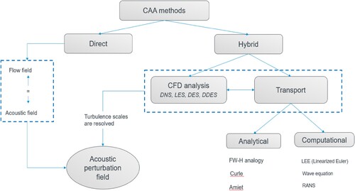
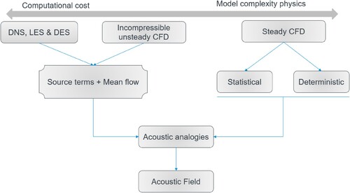
Direct and hybrid methods differ based on the extent or size of the computational domain and numerical discretisation schemes used to resolve the spatial–temporal scales for the flow field and acoustic field, respectively. Direct methods are normally computationally more intensive in terms of time and cost resources involved for any given problem setup. Figure 2 shows the relation between the computational cost and flow physics involved to predict the acoustic field.

Figure 2. Relation between the CAA methods, acoustic analogies and prediction of acoustic field.

1.1. Direct method

In this method, both flow and acoustic fields are computed simultaneously. The physical domain encompasses the source and extends to the region of interest in the near or far-field. The direct method needs a high-resolution computational grid which is spatially resolved in both the flow and acoustic fields. There exists a disparity in scales of flow and acoustic phenomena in practical problems that require long run times and thus inordinate number of computational resources are needed, limiting its applicability to even low Reynolds number simple flow configurations. Also, in this approach, numerical discretisation schemes at high complexity levels are applied compared to traditional schemes used in CFD simulations. Such an approach can produce high dispersion and diffusion errors that often lead to attenuation of acoustic waves, which eventually deteriorates the accuracy of predicted acoustic field (Wagner, Hüttl, and Sagaut 2007; Ferziger and Peric 1998).

Furthermore, the scale-resolving turbulence approaches also impact the nature of the acoustic field (Ferziger and Peric 1998; Zhu, Shen, and Sorensen 2016; Moreau 2021; Nataraj 2022). In this method, the acoustic field can be obtained for all time and length scales using Direct Numerical Simulation (DNS). In Large Eddy Simulation (LES), the acoustic field is computed using the fluctuating component of velocity relative to mean flow field captured at large length scales of motion only while the small scales are approximated using analytical turbulence closure models. However, in both approaches, the statistical properties for turbulence are utilised to predict the accurate flow and acoustic field characteristics.

1.2. Hybrid method

In the hybrid method, the unsteady flow in near-field and far-field acoustic solution is computed with the help of a CFD approach. The sound generated at the source in the near-field is then propagated to the observer in the far-field either by analytical momentum transport equations or or implicitly through artificially dissipation in computational methods. Computational transport methods refer to the case where the governing equations for momentum transport are discretised on a grid external to the CFD source grid and rely on iterative solvers. Analytical transport equations such as the linearised Euler equations or the wave equation, are solved, which are relatively simpler than those solved in the CFD domain. In the analytical hybrid CFD-CAA approach, acoustic analogies are used and based on the integral formulation of the governing acoustic equation, such as the Lighthill and Newman’s (1952) or Ffowcs Williams and Hawkings (FW-H) (1969) equations given in Nataraj (2022; Ffowcs Williams and Hawkings 1969; Zhang, Avallone, and Watson 2022; Lighthill and Newman 1952). Also, hybrid methods can be classified based on turbulent flows encompassing bounded surfaces. For flows without solid boundaries, Lighthills integral formulation is valid for quiescent medium at rest while Howes (2003) acoustic analogy was derived from Powell (1964) theory of vortex-induced sound which essentially couples sound waves with unsteady hydrodynamic flow field properties for jet flows (Powell 1964). Goldstein (2003) proposed acoustic analogy that is based on linearised Navier–Stokes equations in which perturbation of base flow variables such as velocity and pressure are responsible for the production of viscous stress equivalent to Reynolds stress term and heat flux term equivalent to stagnation enthalpy flux in medium. These quantities essentially represent the source terms and become significant for non-radiating base flows which are incompressible and unsteady in nature (Goldstein 2003). For flows that include solid wall boundaries, Curle’s (1955) acoustic analogy is valid for the unsteady flow interaction with stationary solid surfaces only, while FW-H (1969) acoustic analogy is valid for moving surfaces. Acoustic field predicted using FW-H acoustic analogy uses integral Greens function which considers the source region, observer region and a moving boundary surface over which the orthogonal derivative of Greens function vanishes. It can be noted that for incompressible subsonic turbulent flows, without aeroacoustic feedback, the Lighthills analogy predicts acoustic power dependence as eighth power of fluid velocity. Further, for unsteady flows in source region, this analogy predicts noise based on kinematic data of velocity components which can be obtained using Hot Wire Anemometry (HWA), Particle Image Velocimetry (PIV) or Laser Doppler Velocimetry (LDV) measurement techniques. Figure 3 shows the interpretation of FW-H acoustic analogy.

Figure 3. Interpretation of FW-H acoustic analogy in terms of source, observer regions and overlapping envelope surrounding the source and observer.

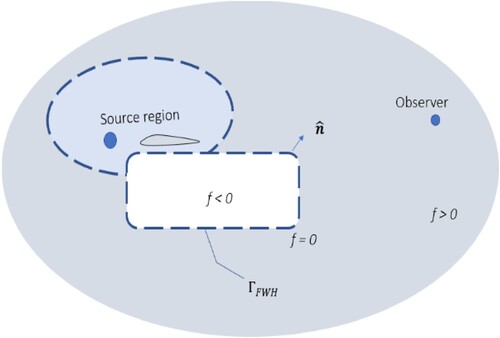
The sound at the observer in the far-field is obtained by computing a surface integral comprising specific source terms. Often the integration surface can be considered as the surface of the object immersed in the fluid defined by control volume which represents all physical phenomena contributing to the far field noise. In a few scenarios, volume integration of specific source terms in the domain external to the integration surface must be carried out because of the relevance of quadrupole sources. It can be said that FW-H and Curle’s, analogies are the most widely used integral methods for predicting acoustic field and considered as formal solutions of Lighthill’s equation applied for rigid and moving wall boundaries relative to flow field. The former includes Lighthill’s stress tensor while in latter it is ignored and hence Curle’s solution can be considered as special case of FW-H analogy. The solution to FW-H acoustic analogy can be obtained in time or frequency domains by computing surface integral over region which encompasses source in near field and observer in far field. The time domain solution can be computed directly by integrating FW-H acoustic transport term given by Equation (2). However, a frequency domain approach requires a solving of a complicated Green’s function for treatment of arbitrarily shaped boundary that includes all noise sources. Zhou et al. (2022) derived the far field approximations to derivatives of Greens function for Ffowcs Williams and Hawkings (FW-H) equations which considers convective wave equation in frequency domain. This approach has been used to predict the sound generated by compressible flows from jet engines (Zhou et al. 2022; Pouangué et al. 2015), propellers (Shur et al. 2003; Poggi et al. 2021), high speed trains (Li et al. 2022; Qin et al. 2022) and hydrofoils (Li et al. 2021). The FW-H equation is a nonhomogeneous wave equation that extends Lighthill’s acoustic analogy to problems with permeable and non-permeable boundaries and given by Equation (2). The density and pressure perturbation terms in the far field are represented by ${\rho }^{\mathrm{\prime }}$ and $p^{\mathrm{\prime }}$. M_i and M_j are the free stream Mach number along directions x and y axis for a given value of free stream velocity, U m/s. H(f) is the Heavyside step function for the permeable or non-permeable boundary, defined by transformation function, f. This function is used to map the geometry of physical domain into computational domain by means of conformal transformation otherwise known as Schwarz-Christoffel transformation and uses the method of images across the boundaries while applying suitable boundary conditions. δ(f) is the Dirac delta function whose value is zero everywhere except where f = 0. T_ij = ρu_iu_j + P_ij – c_o²δij is the Lighthill stress tensor, where u_i is the fluid velocity component along the x-axis. c_o is the speed of sound in ambient medium. P_ij = (p − p_o)δ_ij − τ_ij is the compressive stress tensor. They also investigated the solution to FW-H equation for low Mach number flows in terms of surface integral for monopole, dipole source terms and volume integral for quadpole source term. (2) $\left({\displaystyle \frac{1}{c_o^2}{\displaystyle \frac{{\mathrm{\partial }}^2}{\mathrm{\partial }{t}^2}+M_i{M}_j{\displaystyle \frac{{\mathrm{\partial }}^2}{\mathrm{\partial }{x}_i\mathrm{\partial }{x}_j}+2M_i{\displaystyle \frac{{\mathrm{\partial }}^2}{\mathrm{\partial }{x}_i\mathrm{\partial }t}-{\displaystyle \frac{{\mathrm{\partial }}^2}{\mathrm{\partial }{x}_i\mathrm{\partial }{x}_i}}}}}}\right)(H(f)c_o^2{\rho }^{\mathrm{\prime }})={\displaystyle \frac{{\mathrm{\partial }}^2}{\mathrm{\partial }{x}_i\mathrm{\partial }{x}_j}(T_{ij}H(f))-{\displaystyle \frac{\mathrm{\partial }}{\mathrm{\partial }{x}_i}(F_i\delta (f))+{\displaystyle \frac{\mathrm{\partial }}{\mathrm{\partial }t}(Q\delta (f))}}}$(2) The first three terms of Equation (2) in RHS side are expressed using mapping function, f and represent the quadpole, dipole and monopole sources. It can be noted that prediction methods for acoustic field mentioned previously can be used for various applications such as wind turbine rotors, gas turbines, compressors, fans, hydrokinetic turbines, and jet noise predictions from turbulent flows.

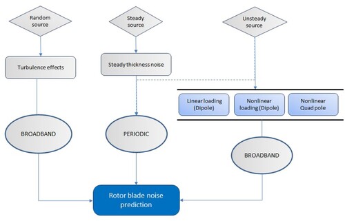
Another approach to classifying noise sources is illustrated in Figure 4. Based on the flow field conditions, a highly random or turbulent source responsible for acoustic radiation can be caused due to interaction of mean flow and fluctuating component of velocity. The fluctuating component is typically much smaller compared to mean flow statistics and characterised by a broad range of frequencies in the noise spectrum. Steady sources include thickness noise caused due to volume flux present in turbulent shear flows, while unsteady sources produce linear or nonlinear loading noise due to external force excitation which are exhibited as dipole or quadpoles in the source and far-field observer regions. Both steady and unsteady types of sources are characterised by specific band of frequencies in noise spectra (Blandeau and Joseph 2011; Yao, Davidson, and Eriksson 2017; Wolf, Kocheemoolayil, and Lele 2014; Wolf, Azevedo, and Lele 2012; Bhargava, Maddula, and Samala 2019).

Figure 4. Illustration of different types of noise sources according to flow conditions.

A well-known analytical model for noise generation from aerofoil in unsteady turbulent flows was developed by Amiet and is based on aeroacoustic transfer function. This function relates scattered acoustic pressure in far field with surface pressure from a trailing edge of linearised thin aerofoil. Further, it expresses the fluctuating lift response function in terms of hydrodynamic wavenumber spectrum for coherent turbulence structures whose dissipation and diffusion time scales are larger and includes incident pressure gusts. An impermeable wall boundary conditions are also applied normal to aerofoil surface along with Kutta condition for trailing edge which eliminates flow singularities. To compute the far-field power spectral density for sound pressure this method applies linearised Helmholtz equation using a mapping function for a given boundary in a repetitive manner to comply with gust–aerofoil interaction problem and known as Schwarzschild technique (Cotte and Tian 2016; Fink 1979). The aim of the present paper, however, is to give an overview on the quasi-empirical models developed for predicting aerodynamic noise generation which is relevant for wind turbines and aerofoils in general.

1.3. Overview of wind energy and acoustic emissions

In the recent past, the world has witnessed an unprecedented increase in the use of renewable energy resources with large-scale power plant installations to curb harmful CO₂ emissions and protect the environment from climate change activities. Among renewable energy sources, wind energy has attracted much attention compared to solar power systems and even the coal-based energy sources due to its operating efficiency, low cost of energy and cleaner production of electricity (Geyer, Sarradj, and Fritzsche 2010). When wind turbines grew bigger in size, noise from moving blades has become critical objectives in wind turbine aerofoil design. From the perspective of social acceptance, the noise aspect becomes very important particular for onshore turbines, such that low-noise wind turbine design is a critical parameter. Hence, detailed understanding aerofoil noise generation mechanisms is essential to make energy extraction more efficient. The wind turbine noise regulation across different countries is based on inhabitants and in Europe stringent laws related to noise levels are applied (Zhu, Shen, and Sorensen 2016). Table 1 shows the wind turbine noise regulation standards and threshold limits during daytime, evening and nighttime for various countries. Hansen et al. (2012) conducted a series of surveys in a field measurement campaign on how wind farm noise is perceived in rural areas both indoors and outdoors of houses. Noise measuring instruments and locations were selected based on the dose–response study which is useful for determining the suitable immission limits. An investigation was also performed on the masking potential of ambient background noise levels during nighttime and daytime based on NZS 6808:2010 and SA (2009) EPA noise guidelines as well as ISO 9613-2 regulation. Regression analysis was conducted on measurement data recorded inside and outside of residences at various microphone locations with at least three statistical datasets for each wind speeds, minimum, maximum and mean values were taken in consideration to determine the difference in sound pressure levels for low frequency and infrasonic noise sources. SPL differences up to 30 dB of noise reduction between indoors and outdoors with windows closed were observed while a 15 dB noise reduction was found when the window was open. In a similar investigation done by Hubbard and Shephard (1991), atmospheric propagation and building response models were considered. It was found that for high frequencies, atmospheric attenuation factors like refraction showed a further reduction up to 2 dB within shadow zones upwind of source and for low frequencies attenuation was observed downwind with a reduction potential up to 3 dB. The attenuation rates were found to be −3 dB per doubling of distance assuming cylindrical spreading and −6 dB assuming spherical spreading for distances up to 1200 m. In building response model, human perception for noise and noise-induced vibrations inside the dwellings were considered to suggest that measured sound pressure level are subjected to variations that depend on the cavity resonances between the rooms (Hubbard and Shephard 1991).

Table 1. General and wind turbine noise regulation standards and thresholds in different countries (Bhargava and Samala 2019a).

Country	Lp-d	Lp-n	ΔLpd-n	Regulation
India
Industrial zone	75	70	5	CPCB – 1993
Commercial zone	65	55	10
Residential zone	55	45	10
Special zone	50	35	15
China				GB 12523-2011^ϯ
Industrial zone	65	55	10	GB 12348-2008*
Traffic zone				GB 22337-2008^×
Road	70	55	15
Railway	70	60	10	CCAR – 36
Aircraft*	80	74	6
Residential zone
Plane	60	50	10
Mixed	55	45	10
Special zone	50	40	10
Germany	40	35	5	See Bastasch et al. (2006) ETSU-R-97
Denmark^+	44 @ 8 m/s; 42 @ 6 m/s
Canada/US	40–51 dB(A) 43 dB(A) + 5 dB (A) at evening; + 10 dB (A) at night 35/40 dB(A) + 5 dB(A) at night
UK
Australia

Noise metrics: L_pA = Aweighted perceived noise level; L_pd = Day time level; L_pd = Night time level; L_pd = Average of day and night time level; L_Aeq = A weighted equivalent continuous level; L₉₀, L₁₀ refers to background noise levels with 10% and 90% exceedance in measured data.

ϮConstruction.

×Community.

*Hong Kong international airport.

2. Noise mechanisms from wind turbine blades

Broadly the noise generated by wind turbines can be classified as aerodynamic and mechanical noise, however, a more subtle classification on noise from the wind turbines is based on the frequency range and amplitude levels in noise spectra (Zidan, Elnady, and Elsabbagh 2014)

• A tonal noise occurs at discrete frequencies and is caused by the wind turbine components such as meshing of gears, interaction of blade surface with stable boundary layer and from vortical flow expansion from thicker trailing edge sections.

• Broadband noise is caused by edge scattering of turbulent flows over the moving blade and becomes significant when the frequency is in the range 100 Hz–5 kHz.

• A low-frequency noise occurs in the frequency range 20-200 Hz that exhibits both broadband and impulsive type noise characteristic and caused due to amplitude modulation of acoustic pressure waves generated from wind turbine blades.

• The low frequency impulsive noise is characterised by a ‘thump’ in far field and a sudden flow separation that occurs from leading edge of wind turbine blades is the prime reason for this type of source. On the contrary, low frequency broadband noise is characterized by ‘whomp’ that results when the turbulent boundary layer flows over the trailing edge of blade.

• An infrasonic noise is considered as thickness noise source which occurs if the 1/3rd octave frequency is below 20 Hz. When the blade encounters turbulent eddies produced by tower wake this type of source exhibits stronger amplitude modulation depths and cause anxiety, stress-related effects in human beings.

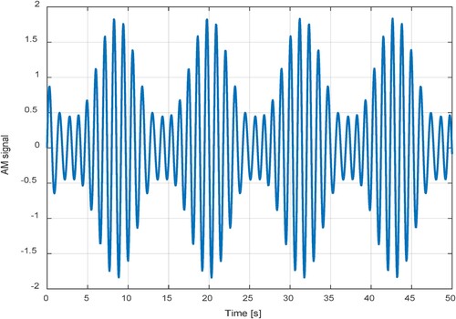
Amplitude modulation is one of the most important characteristics from the perspective of wind turbine noise due to change in amplitude of sound pressure level at blade passing frequencies. The extent of amplitude modulation is determined using modulation depth measured between extremes of sound pressure waves in atmosphere. As the modulation depth increases, the amplitude modulation also increases in logarithmic manner. Also, this phenomenon can occur at both infrasonic and low frequency noise from wind turbines producing a beating sound character. According to Van den Berg (2006), this beating nature is quantified by modulation depth which is stronger during nighttime due to stable atmospheric conditions and results in persistent annoyance for inhabitants living near wind farms (Van den Berg 2006). Several factors are responsible for amplitude modulation which includes turbine design, wind speed, topography and directional aerodynamic noise sources from rotor blade. In addition, stable and neutral atmospheric conditions potentially affect amplitude modulation during nighttime and daytime periods. As mentioned before, trailing edge noise source is modulated at blade passing frequencies and strength of amplitude modulation varies with atmospheric turbulence properties. To represent the theoretical application of amplitude modulation relevant to wind turbine noise assessment a simple analysis considering carrier tone signal with a frequency of 50 Hz and sine wave modulation signal with sensitivity of 0.8 was done. Figure 5 illustrates the amplitude modulation of signal obtained using superimposition of the carrier and modulation signals represented by Equations (3) and (4) given in (Cooper 2021) (3) $c(t)=A_c\sin (2\pi f_{c}t)$(3) (4) $M(t)=A_m\sin (2\pi f_{m}t)$(4)

Figure 5. Resultant amplitude modulation of signal, f with a phase angle of 90° obtained using superimposing carrier signal (f_c = 50 Hz, A_c = 1), and modulation signal, f_m at modulation index, m = 0.9.

The resultant modulated signal can be expressed in form of Equation (5) (5) $Y(t)=A_c\sin (2\pi f_{c}t)[1+A_m\sin (2\pi f_{m}t)]$(5)

2.1. Types of noise sources

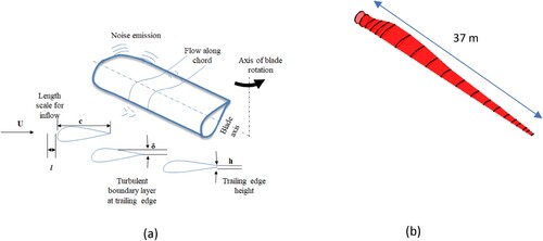
In Figure 6(a,b), the predominant aeroacoustics noise sources from an aerofoil and wind turbine blade are

• Turbulent boundary layer trailing edge noise (TBL-TE).

• Separation stall noise.

• Tip noise from vortex flows.

• Vortex shedding noise due to trailing edge geometry (TEB-VS).

• Inflow noise (TI).

Figure 6. (a) Flow-induced noise sources from an aerofoil (Bhargava and Samala 2019b). (b) Illustration of wind turbine blade length (Bhargava and Samala 2019a).

Several theoretical studies on aerofoil self-noise focused on leading and trailing edge noise generated by a two-dimensional flat plate or a semi-infinite thin aerofoil. Broadband leading-edge noise is produced when turbulent packet of air interacts with moving boundaries or surfaces to develop elastic or pressure waves. On the other hand, trailing edge noise is caused when the turbulent boundary layer flows undergoes edge diffraction over finite impedance surfaces. However, most experimental studies that involved aerofoils were usually wall-mounted and finite in length which resemble that of wind turbine blades attached to a hub, or ship hydrofoils attached to a hull. The flow field around a wall-mounted finite aerofoil is complex and features several three-dimensional fluid phenomena due to boundary layer effects (Moreau 2021; Li et al. 2021; Shen et al. 2019; Tang, Lei, and Fu 2019; Kingan 2005; Brooks and Hodgson 1981). Depending on the strength of bound circulation and flow angle of attack, the boundary layer on pressure or suction side of aerofoil forms a vortex system and extends into the wake. A vortex system can be seen to emerge from an edge of a finite span aerofoil and responsible for tip noise production (Ikeda et al. 2013; Yao, Davidson, and Eriksson 2017; Wolf, Kocheemoolayil, and Lele 2014; Wolf, Azevedo, and Lele 2012). It can be said that aerofoil thickness to chord ratio and aspect ratio are some of the important geometric factors which can affect the vortex formation while aerodynamic flow conditions governed by Reynolds number and Strouhal number affect the trailing edge noise. For horizontal axis wind turbine blades, an important source of noise comes significantly from the outer third length of blade during downward direction of motion. Also, for downwind turbines, the interaction of leading edge of moving blade with turbulent eddies produced by tower wake generates impulsive type noise periodically and propagates to far-field observer. This type of noise is dominant in low or infrasonic frequencies in SPL spectra. Similarly, sound is also radiated when trailing edge of rotor blade interacts with turbulent flow to result in high-frequency broadband noise which is sometimes known as swish (Doolan et al. 2012). In the next section, we discuss the quasi-empirical methods for predicting noise from wind turbine rotors.

2.2. Quasi-empirical methods for noise prediction

As described in Section 1.1 and 1.2, methods for acoustic field prediction rely on numerical CFD-based techniques as well as analytical formulations for resolving turbulent flows that are responsible for flow-induced noise in near or far field. These methods have been applied extensively for predicting aerodynamic noise from rotating machinery such helicopter blades, compressors, fans owing to its highly accurate results. CFD-based methods typically use RANS or LES solvers to compute the full flow field statistics required to predict the acoustic field from a noise source. In this section, we discuss some of the widely applied quasi-empirical methods for predicting flow-induced noise from aerofoils and wind turbine blades.

2.2.1. Brookes, Pope and Marcolini (BPM) model

Brooks, Pope, and Marcolini (1989) developed model for aerofoil self-noise mechanisms based on wind tunnel experiment data obtained for series of test data of thin symmetric aerofoils with chord length ranging from 2.5 cm to 60 cm. NACA0012 aerofoil was chosen and modelled as half infinite flat plate structure. The empirical derived expressions for far-field sound pressure level constitute geometry properties of aerofoils and boundary layer parameters such as thickness, displacement thickness as function of chord length and angle of attack. Also, a directivity function was included to analyse the effect of sound field radiation close to source. Furthermore, in this model, the aerofoil self-noise is predicted using the logarithmic scaling of turbulent boundary layer parameters, predominantly displacement thickness δ*, Mach number M, high-frequency directivity function D_h distance between the source and receiver r_e, blade span length L, and spectral shape functions A and B depend on the Strouhal number, St. Also, the sound pressure levels vary with fifth power of local velocity or free stream Mach number, M⁵ and with chord Reynolds number, Re_c. The broadband spectrum of acoustic pressure is divided into three components viz. pressure side source which uses directional expression and appears dominant in high-frequency region, suction side source exhibits peak towards low-frequency part of spectrums. Both the sources are found to vary negligibly with angle of attack (AOA). The stall separation noise is critical to AOA and produces peaks at moderate to large positive values of AOA. This noise source reduces to a compact dipole and uses low-frequency directivity function. The flow separation noise also occurs for high positive AOA for which high-frequency directivity is used. The three noise sources are added logarithmically along the individual blade segments to obtain resultant overall SPL. The empirical equations involved to evaluate the SPL are given by Equations (6)–(9) (6) $\mathrm{SP}{\mathrm{L}}_{\mathrm{p}}=10\cdot \log \left[{\displaystyle \frac{{\delta }_p^{\ast }{M}^{5}L\overline{D_h}}{r_e^2}}\right]+A\left[{\displaystyle \frac{S{t}_p}{S{t}_1}}\right]+[K_1-3]+\mathrm{\Delta }{K}_1$(6) (7) $\mathrm{SP}{\mathrm{L}}_{\mathrm{s}}=10\cdot \log \left[{\displaystyle \frac{{\delta }_s^{\ast }{M}^{5}L\overline{D_h}}{r_e^2}}\right]+A\left[{\displaystyle \frac{S{t}_s}{S{t}_1}}\right]+[K_1-3]$(7) (8) $\mathrm{SP}{\mathrm{L}}_{\alpha }=10\cdot \log \left[{\displaystyle \frac{{\delta }_s^{\ast }{M}^{5}L\overline{D_h}}{r_e^2}}\right]+B\left[{\displaystyle \frac{S{t}_s}{S{t}_2}}\right]+K_2$(8) (9) $\mathrm{SP}{\mathrm{L}}_{\mathrm{Total}}=\sum _{i=1}^{N}10\cdot \log \left[{10}^{{\displaystyle \frac{\mathrm{SP}{\mathrm{L}}_i}{10}}}\right]$(9) (10) $\mathrm{SP}{\mathrm{L}}_{\mathrm{Blunt}}=10\cdot \log \left[{\displaystyle \frac{h{M}^{5.5}L\overline{D_h}}{r_e^2}}\right]+G_4\left({\displaystyle \frac{h}{{\delta }_{\mathrm{avg}}^{\ast }},\phi }\right)+G_5\left({\displaystyle \frac{h}{{\delta }_{\mathrm{avg}}^{\ast }},\phi ,{\displaystyle \frac{S{t}^{\mathrm{\prime }}\mathrm{\prime }\mathrm{\prime }}{S{t}_{\mathrm{peak}}^{{}^{\mathrm{\prime }}\mathrm{\prime }\mathrm{\prime }}}}}\right)$(10) (11) $\mathrm{SP}{\mathrm{L}}_{\mathrm{Tip}}=10\cdot \log \left[{\displaystyle \frac{M_{max}^3{M}^2{l}^2\overline{D_h}}{r_e^2}}\right]-30.5(\log St\mathrm{\prime }\mathrm{\prime }+0.3{)}^2+126$(11) K₁ and K₂ are amplitude constants and ΔK₁ is the amplitude peak adjustment constants, the high-frequency directivity, D_h proposed by Fink (1979) is expressed in terms of trailing edge noise directivity, $\mathrm{si}{\mathrm{n}}^2(\theta /2)$, convective amplification and Doppler shift functions are given by $[1+(M-M_c\cos \theta ){]}^2$ and $1+(M\cos \theta )$ exhibit the directional nature of sound during the downward motion of blade relative to the receiver position. The coordinate systems are required to be shifted or transformed to account for the relative position of moving source with respect to fixed observer. Due to rotor rotation, about the horizontal axis the noise spectrum also needs to be averaged around azimuth direction to predict the overall sound pressure level. Equations (10) and (11) represent the SPL spectra for vortex shedding noise from trailing edge and tip noise produced from turbulent vortex flow at the tip of blade.The tip noise depends on the geometry of tip shape, a square or blunt tip produces higher noise level compared to round or sharp tip. The BPM model predicts that tip noise levels also vary with strength of tip vortex produced at given free stream velocity. G₄ and G₅ are spectral functions expressed in terms of trailing edge thickness and average boundary layer displacement thickness from pressure and suction sides of aerofoil. G₄ represents the sharp peak in high-frequency region of acoustic spectrum and G₅ is a shape function for determining broadband characteristics in SPL spectra (Zhu 2004; Moriarty and Migliore 2003; Wei et al. 2016; Grosveld 1985). M_max is the maximum Mach number achieved on the surface of aerofoil or blade. It is also noted that acoustic measurements for turbulent boundary layer trailing edge self-noise from aerofoils were assumed to have uniform inflows and a fast Fourier transform was applied to determine the cross-correlation of noise data from microphones to account for spectral scaling for zero and non-zero angle of attacks as well as for boundary layer in tripped and un-tripped conditions. This helped overcome the problem of convective turbulence in subsonic flows over flat plates and aerofoils. Equations (6)–(8) and Equation (10) are obtained from the scaled and normalised form of one-third octave SPL spectra given by Equations (18) and (19) in (Brooks, Pope, and Marcolini 1989). For laminar boundary layer instabilities, no scaling was used but instead the frequency dependence of the SPL spectra was found to scale with Strouhal number based on boundary layer thickness to determine the one-third octave SPL spectra. The resulting normalised LBL-VS noise spectrum in one-third octave format is given by Equation (12) (12) $\mathrm{SP}{\mathrm{L}}_{\mathrm{LBL}\text{-}\mathrm{VS}}=10\cdot \log \left[{\displaystyle \frac{h{M}^{5}L\overline{D_h}}{r_e^2}}\right]+G_1\left({\displaystyle \frac{S{t}^{\mathrm{\prime }}}{S{t}_{\mathrm{peak}}^{\mathrm{\prime }}}}\right)+G_2\left({\displaystyle \frac{R_c}{R_{c0}}}\right)+G_3({\alpha }_{\ast })$(12) where G₁ refers to overall spectral shape function matching the one-third octave SPL level, G₂ represents the scaled peak spectra noise level which vary with chord Reynolds number, R_c. G₃ is angle-dependent noise level as function of G₂.

Thus, the normalised and scaled SPL level for TBL-TE, trailing edge bluntness vortex shedding (TEB-VS) and laminar boundary layer vortex shedding (LBL-VS) noise mechanisms can be written in general form given by Equation (13) (13) $\mathrm{Scaled}\mathrm{SPL}=\mathrm{SP}{\mathrm{L}}_{\mathrm{\varnothing }}-10\cdot \log \left[{\displaystyle \frac{M^{5}LX}{r_e^2}}\right]$(13) where ϕ represents the SPL functional parameter based on angle of attack, α, Strouhal number frequency scaling on boundary layer thickness or displacement thicknesses from pressure or suction sides from aerofoils. X represents relevant length scale based on the boundary layer parameter.

2.2.2. Grosveld model

According to the Grosveld (1985) method, acoustic waves are produced due to impingement of boundary layer turbulence over an aerofoil. Modern turbine blades are twisted and have varying chord lengths along each blade segment of length l. So, local velocities over each segment experience unsteady blade lift and drag forces due to varying inflow angles. However, this model assumes linearly tapered rotor and ignores twist and therefore appropriate corrections for inflow and angle of attacks are not considered as in the case of BPM. In potential flows, the trailing edge noise from aerofoil can be calculated using Equation (14) (14) $\mathrm{SP}{\mathrm{L}}_{\mathrm{p}}=10\cdot \log 10\left[{\displaystyle \frac{B\delta U^{5}L\overline{D_h}}{r_e^2}\cdot K{K}_2}\right]$(14) where KK₂ is the frequency-dependent scaling function and given by Equation (15) (15) $KK2(f)=10\cdot \log 10\left[\left\{{\left({\displaystyle \frac{S{t}^{\mathrm{\prime }}}{S{t}_{max}}}\right)}^4\right\}{\left[{\left({\displaystyle \frac{S{t}^{\mathrm{\prime }}}{S{t}_{max}}}\right)}^{1.5}+0.5\right]}^{-4}\right]$(15) where St_max and St′ are maximum Strouhal number set to ∼0.1, and scaled with δ, B is blade count in rotor and U is the velocity scaled to U⁵. Further, it also uses a directional approach function D_h and boundary layer thickness. The thickness of turbulent boundary layer, δ, can be evaluated using data fitting technique for chord c of aerofoil (Grosveld 1985). The modulating amplitude of acoustic waves caused due to convection in turbulent flows is set equal to 0.8 times the Mach number and shows dipole nature of noise radiation orthogonal to the rotor plane. The overall noise level is obtained by integrating the noise from each blade segment logarithmically. In addition, noise levels from different wind turbine sizes from sub-megawatt to multi-megawatt for fixed and varying operating conditions were investigated. For turbulent inflow noise source, Grosveld (1985) proposed a inflow turbulent noise model which predicts noise from rotating blades of wind turbines as a result of fluctuating loads in rotor plane. The unsteady blade loading in rotor plane is attributed to factors such as change in the angle of attack, length scale and turbulence intensity from a specific height above ground. The inflow turbulence noise model is based on theory developed for helicopter rotor noise which uses the homoegeneous isotropic turbulence spectrum integrated between the minimum and maximum frequency regions, given by Equation (2) to Equation (5) in Grosveld (1985). For far-field noise prediction, this model utilises the aerodynamic transfer function approach in which noise sources are assumed as point dipoles located at the hub centre to yield the rms sound pressure level and given by Equation (10) in (Grosveld 1985). Furthermore, the model is also extended to predict the fluctuating surface pressure across blunt trailing edges of an aerofoil which is responsible for causing vortex-shedding noise. Following the scaling laws used in BPM model presented in Section 2.2.1 the one-third octave SPL levels in far field are found to be dependent on the ratio of trailing edge height and displacement thickness, δ* as well as frequency-dependent constants and given by Equations (29)–(33) in Grosveld (1985).

2.2.3. Lowson model

Using this method, the noise level is calculated using scaled dimensional factor technique based on experiment data done by BPM discussed in Section 2.2.1. The sound pressure level is evaluated using the spectral functions like BPM method; however, the empirical constants for scaled SPL are found to depend on the boundary layer thickness, Strouhal number and Mach number for different flow regimes. Compared to BPM technique, a constant factor of 128.5 was introduced in this method to obtain the scaled SPL value that will allow to estimate combined noise level from both suction and pressure sides of aerofoil. The frequency-dependent scaling factors that are used to determine the sound pressure level are given by Equations (16) and (17) (16) $\mathrm{SP}{\mathrm{L}}_{\mathrm{p}}=10\cdot \log 10\left[{\displaystyle \frac{\delta M^{5}L}{r_e^2}\cdot G_6(f)}\right]+128.5$(16) (17) $G_6(f)={\displaystyle \frac{4{\left({\displaystyle \frac{f}{f_{\max }}}\right)}^{2.5}}{{\left[{\left({\displaystyle \frac{f}{f_{\max }}}\right)}^{2.5}+1\right]}^2}}$(17) where f_max is dependent on free stream Mach number, M is given by U/c, U is fluid flow velocity over the blade surface, δ is boundary layer thickness (Zidan, Elnady, and Elsabbagh 2014). Lowson (1992) also derived an empirical relation for turbulent inflow noise which is based on the Amiet’s experiment measurements of surface pressures on the thin aerofoils and flat plates. This model can be applied for broad range of frequencies in SPL spectra in which turbulence properties were approximated using homogeneous isotropic turbulence von-Karman spectra relating the surface boundary layer measurements with acoustic field. The turbulent flow properties were characterised based on rms value of velocity fluctuations, turbulence wave number of energy-containing turbulent eddies, integral length scale and turbulence intensity (Lowson 1992). The overall expression for terms in inflow noise prediction is given by Equation (18)–(21) (18) $\mathrm{SP}{\mathrm{L}}_{\mathrm{in}}=\mathrm{SP}{\mathrm{L}}_{\mathrm{H}}+10\cdot \log \left[{\displaystyle \frac{\mathrm{LFC}}{1+\mathrm{LFC}}}\right]$(18) (19) $\mathrm{SP}{\mathrm{L}}_{\mathrm{H}}=10\cdot \log \left[{\displaystyle \frac{{\rho }^2{c}^{2}lL}{2r^2}{M}^3{u}^2{I}^2{\displaystyle \frac{K^3}{{(1+K^2)}^{{\displaystyle \frac{7}{3}}}}{D}_L}}\right]+78.4$(19) (20) $\mathrm{LFC}=10S^{2}M{K}^2{\beta }^{-2}$(20) (21) $S^2={\left({\displaystyle \frac{2\pi K}{{\beta }^2}+{\left(1+2.4{\displaystyle \frac{K}{{\beta }^2}}\right)}^{-1}}\right)}^{-1}$(21) where $\beta =\sqrt{1-M^2}$ and $K={\displaystyle \frac{\pi fc}{U}}$, where, LFC is low-frequency correction factor involving the compressible aeroacoustic sears transfer function, S, which varies with acoustic wave number K. L is the span length of aerofoil source and I is the turbulence intensity, l is the integral length scale parameters and r is the total or effective distance between the observer and source. As mentioned earlier, the model constitutes the low-frequency directivity function and high-frequency corrections for TI noise in which high-frequency correction involves isotropic von-Karman turbulent velocity spectra along with empirical constants to take account of limitation of Amiets model related to observer position or location in measurement of sound pressure over a frequency range, 200–2500 Hz in SPL spectra. The low-frequency corrections involve the spherical directivity and depend on the compressible sears function to analyse the effect of periodic and random gusts in turbulent flow field. To take account of compressibility effects of turbulent flows on generation of acoustic field, it also considers the Prandtl–Glauert compressibility criterion as function of Mach number, M and given by β. D_L is the low-frequency directivity function expressed in terms of observer angles in the rotor and azimuthal planes, respectively.

2.3. Rotational harmonics

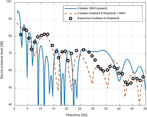
As mentioned in beginning of Section 2, wind turbines operating in open environments exhibit amplitude modulation of sound pressure level at blade passing frequencies which means the number of blades play an integral role in rotational harmonics in overall noise level perceived by inhabitants near wind turbines. Hubbard and Shephard (1991) have investigated amplitude modulation for two and three-bladed large-scale wind turbines. The broadband SPL spectrum for downwind and upwind turbine rotors in low and mid-band frequency range, 20 Hz < f < 2 kHz was computed based on the analytical closed form solutions for predicting rotational noise from helicopter rotors. To predict near field flow induced noise at higher harmonics an empirical relation was derived as function of tip speed and swept area of rotor. However for predicting far field noise, unsteady rotor blade loading of turbine torque and thrust derived using complex Fourier coefficients given by Equation 8b in Lowson (1970) was implemented. It was found that SPL modulation amplitudes varied over time scales for a single rotor revolution measured at 150 m and 183 m distance from the source. The downwind rotor had a diameter of 79 m while upwind rotor had 92 m and measured sound pressure signals from upwind rotor was found to vary in a cyclically manner with a phase difference of 180° compared to upwind rotor when blades moved past the tower. Further, intermittent SPL peaks were found at frequencies f ∼ 600 Hz and f ∼ 1.2 kHz which are believed to be caused from gearbox or cooling fan noise inside the nacelle of the turbine. Additionally, rotational harmonics at infrasonic and low frequencies for downwind rotors are stronger compared to upwnd rotors. Also, for both upwind and downwind rotors the generator shaft harmonics were found to emit tonal noise peaks at high frequencies that varied with integral multiples of blade passing frequencies (Hubbard and Shephard 1991).

It can be noted that rotational harmonics are a function of integral multiples of blade passing frequency which result in radiation of acoustic pulses in far field. The acoustic pulses are attributed to unsteady blade loads due to rapid changes in the lift and drag forces over the blade surface in rotor plane. This variation in blade loading was computed using the Sears function in terms of complex Fourier coefficients which considers the sinusoidal gusts in wind field. A generalised expression for RMS sound pressure level for upwind and downwind rotors proposed by Viterna (1981) is given by Equation (22) (22) $P_{rms,n}={\displaystyle \frac{\sqrt{2}\sin \gamma }{4\pi R_{e}d}{M}_n^2\sum _m{e}^{im\left(\mathrm{\varnothing }-{\displaystyle \frac{\pi }{2}}\right)}{J}_x\left(a_m^T\cos \gamma -{\displaystyle \frac{nB-m}{M_n}{a}_m^Q}\right)}$(22) where M_n = nB ${\displaystyle \frac{R_e\mathrm{\Omega }}{a_o}}$, m is the blade loading harmonic index, n is the sound pressure harmonic, P_rms,n is the rms sound pressure for nth harmonic, B is the number of blades, Ω is rotor speed in rpm, c_o is the speed of sound, J_x is the Bessel function of first kind and order x, R_e is the effective blade radius, d is distance from rotor hub, ϒ is the blade azimuth angle, ϕ is the altitude angle to receiver, $a_m^T$ and $a_m^Q$ are the complex Fourier coefficients for thrust and torque acting on the turbine rotor (Hubbard and Shephard 1991; Lowson 1970).

Figure 7 demonstrates the comparison of sound pressure level varying with harmonic number, n computed at frequency resolution, Δf value of 0.25 Hz, following the Viterna (1981) approach. It can be observed that for three-bladed turbines, peaks at low frequencies are closely spaced showing a logarithmic decrease in pressure amplitudes and agree well with experiment data of Hubbard and Shephard (1991). As the frequency increased, the peaks are spaced wider apart with reduction in amplitudes which are found to deviate with experiment data by more than 5%. However, for two-bladed turbines, sound pressure peaks appear equidistant for integral multiples of blade passing frequencies. Also, it may be noted that noise radiated in rotor plane shows a strong correlation with strength of wake produced downstream of tower and is known as blade tower interaction (BTI) reinforcement. When turbines operate in a large array, this phenomenon is found predominant in downwind turbines compared to upwind turbines of similar size and tend to increase the sound pressure level by 6 dB. A similar effect of amplitude modulation known as swish reinforcement is observed from the trailing edge of blade surface as discussed in Section 2.1.

Figure 7. Illustration of sound pressure level varying with harmonic number, n, at wind speed of 13.5 m/s compared to experiment data measured downwind at distance of ∼100 m for (Δf = 0.25 Hz).

3. Past research findings

Most important quasi-empirical results were obtained by Brookes Pope Marcolini (BPM) in which the five self-noise mechanisms were modelled using specific properties of boundary layer. That included turbulent boundary layer trailing edge noise, stall separation noise, tip noise and vortex shedding from blunt trailing shapes (Bhargava, Samala, and Anumula 2019). An extensive database was developed by testing seven NACA 0012 aerofoil blade sections of different chord lengths up to 61 cm for different wind tunnel test speeds up to Mach 0.2, angle of attack that ranged between 0° and 25° and the flow Reynolds number that varied between 2 and 5 million.

Figure 8 shows the combined plot for measured aeroacoustic data for NACA0012 aerofoil. A comparison for the sound pressure level (SPL) has been made with other test parameters which include chord length, free stream velocity, angle of attack and one-third octave centre frequency. The data for SPL is clustered at lower values of one-third octave frequencies but scattered for high frequencies in SPL spectra indicating that SPL is more sensitive to changes at low frequencies relative to mean flow velocity. On the other hand, at high frequencies and at constant angle of attack the SPL is less sensitive. As illustrated in Table 2, the mean SPL and angle of attack for self-noise data are found to be 124.83 dB and 6.7° at free stream velocity of 50.9 m/s.

Figure 8. Experimental data for NACA 0012 aerofoil self-noise recorded in a wind tunnel for different test configurations (Sabat et al.).

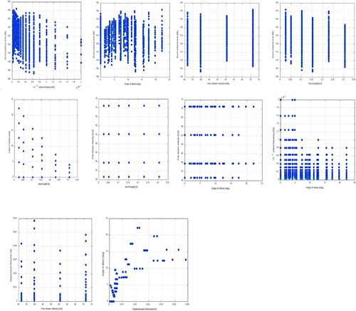
Table 2. Statistical descriptors for the aerofoil self-noise data (Viterna 1981).

Parameter	Mean	Std deviation	Min	Max	25%	50%	75%
Frequency (Hz)	2886.38	3152.57	200	20,000	800	1600	4000
Angle of attack (deg)	6.782	5.918	0	22.2	2.0	5.4	9.9
Chord length (m)	0.1365	0.0935	0.0254	0.3048	0.1016	0.1016	0.2286
Free stream velocity (m/s)	50.86	15.572	31.7	71.3	39.6	39.6	71.3
SPL (dB)	124.835	6.898	103.380	140.987	120.191	125.721	129.995

Moriarty and Migliore (2003) did a series of noise prediction routines at National Renewable Energy Laboratory (NREL) to calculate the total aeroacoustic signature of aerofoils and full-scale operating wind turbines. They conducted a validation study using a series of wind tunnel tests to predict the sound pressure spectra for 2D NACA0012 aerofoil. A difference in noise amplitudes up to 6 dB was found between measured and predicted data under changing flow conditions. Parametric studies and measurements were conducted on Atlantic Orient Corporation (AOC), 50 kW small scale wind turbine model to verify the sensitivity of measured and predicted sound pressure levels. The predicted noise levels were dominated by inflow turbulence noise that is sensitive to changes in the turbulence intensity and length scale (Moriarty and Migliore 2003; Wei et al. 2016). Similarly, Buck, Oerlemans, and Palo (2018) conducted a parametric study on the turbulent inflow over moving blade of an experimental full-scale 2.3 MW-108 m Siemens wind turbine. They investigated an empirical model that is basically a modification of Amiet model for flat plate which was further extended by Lowson (1992) for inflow noise prediction. The conservation of mean flow quantities and turbulent energy dissipation rate in flow field was used to predict the turbulent inflow noise from the blade instead of commonly used integral length scale and turbulence intensity approach. Further, they suggested empirical corrected expressions for aerofoil thickness to cross validate the experiment data of sound pressure collected for 50 hours duration having a turbulence intensity between 8% and 30% with siemens xNoise prediction code. The results showed a prediction error of 3–5 dB for overall inflow noise and less than 3 dB for thickness correction. In a comprehensive study by Schlinker and Amiet (1981), a detailed understanding about the influence of turbulence on helicopter rotor noise, it was found that in turbulent flows, vortices were considered as discrete hairpin filament-like structures at high angle of attacks and boundary layer velocity profile trends did not match with measurements at distance from the boundary (Geyer, Sarradj, and Fritzsche 2010; Brooks, Pope, and Marcolini 1989; Blandeau and Joseph 2011). This may imply that vortex shedding phenomenon on blades is also linked strongly to spanwise turbulent flow conditions in the rotor plane. Moreau, Roger, and Christophe (2009) investigated different types of aeroacoustic noise mechanisms from highly loaded aerofoils and blades for attached and fully separated flow characteristics. It also included geometries from a simple flat plate to thick aerofoils under different flow regimes, e.g. free stream velocities up to 33 m/s and Reynolds number up to 1.5 × 10⁵ (Oerlemans, Sijtsma, and Lopez 2007). They measured far-field sound at midspan of aerofoils and normal to aerofoil chord by using set of directional microphones, which was aimed to capture wall pressure statistics. Wei et al. (2016) investigated the different types of optimised aerofoil designs using trigonometric functions for mitigating the noise as well as to improve the high lift-drag ratio from aerofoil. They used DTU-LN1xx, LN2xx and LN3xx aerofoil families as baseline aerofoils and Xfoil for modelling different flow conditions, e.g. varying Reynolds number from 1.6 million to 16 million, angles of attack between 3° and 10°. Further CFD-based models, Q³UIC, EllipSys and BPM programme were utilised for validating the design results with cross computations (Zhu, Shen, and Sorensen 2016). In addition, an improved method for trailing edge bluntness noise was proposed based on original BPM model to predict the high frequency peak in SPL spectra more accurately.

Oerlemans, Sijtsma, and Lopez (2007) performed a parametric study on detection of aeroacoustic sources on aircraft and wind turbines using phased microphone arrays. A semi-empirical noise prediction method was developed to assess the influence of blade geometry and operating conditions of wind turbine to correlate with measured sound pressure level. A good agreement was found between experiment and predicted noise data for various noise source distributions in rotor plane. Acoustically optimised aerofoils were also tested that included trailing edge serrations on the turbine blades. Measurements for the far-field sound pressure levels were done using microphone arrays to predict the overall noise signature of turbine.

Similarly, low noise optimisation studies by Tang, Lei, and Fu (2019; Kingan 2005; Leloudas 2006; Moreau, Brooks, and Doolan 2011; Ikeda et al. 2013; Hansen 2012) also demonstrated that a 2–5 dB noise reduction can be achieved when the aerofoils are equipped with special features such as porosities on the surfaces, trailing edge serrations. This suggests that noise levels are sensitive to changes with aerofoil surface, geometric patterns, and flow conditions at the trailing edge of aerofoils. Table 3 shows important past research findings related to aerofoil self-noise mechanisms for different flow conditions.

Table 3. Summary of past research findings related to aerofoil self-noise prediction methods.

Year	Author(s)	Summary/finding(s)	Source
1973, 1976	Paterson et al (1973), Paterson and Amiet (1976)	Conducted an experiment study on tonal noise characteristic which correlated boundary layer stability using boundary layer thickness and periodic vortex shedding frequencies. Formulated a theoretical model for surface pressure which can predict the far field noise based on inflow turbulence parameters and also validated the model with experiment data measured on 23 cm chord NACA 0012 aerofoil.	Journal of Aircraft (Paterson et al. 1973) NASA report, CR-2733
1974	Tam	Studied tonal noise using wind tunnel experiments and highlighted that self-excited aeroacoustic feedback loop is caused due to wake instabilities in laminar boundary layer from pressure side of aerofoil. Transient oscillations of acoustic waves in far field were found to dependent on near field pressure perturbations.	Journal of Acoustical Society of America (Tam 1974)
1981	Shlinker and Amiet	Studied helicopter rotor noise prediction techniques based on turbulence boundary layer theory and developed analytical formulations using spanwise flow coherence correlations on blades. Showed that spanwise flow coherence relations strongly influenced far field rotational noise prediction.	NASA CR 3470 (Schlinker and Amiet 1981)
1983	Arbey and Bataille	Found that broadband noise spectra for laminar flows are attributed to edge diffraction of T-S waves instabilities at leading edge to produce discrete tones. Investigated the self-excited aeroacoustic feedback loop and position of maximum velocity point along chord length of aerofoil.	Journal of Fluid Mechanics (Arbey and Bataille 1983)
1999	Nash, MacAlpine et al.	Investigated tonal noise characteristics based on boundary layer flow separation mechanisms that couple acoustic waves travelling upstream of trailing edge of aerofoil along with T-S wave instabilities downstream of chord. This is based on work proposed by Tam (1974)	Journal of Sound and Vibration (McAlpine, Nash, and Lowson 1999)
1989	Brookes, Pope and Marcolini	Developed the semi empirical noise model for prediction of aerofoil self-noise mechanisms using measured wind tunnel test data and curve fitting techniques. Used aerofoils of chord length up to 60 cm in wind tunnel tests and validated SPL spectra at Mach numbers ranging from 0.1 to 0.6.	NASA reference publication 1218 (Brooks, Pope, and Marcolini 1989)
2003	Moriarty and Migliore	Extended the BPM model and investigated aerofoil self-noise mechanisms for small-scale wind turbines and aerofoils. Validation for sound pressure were found to deviate by 6 dB for high Re flows compared to predicted results.	NREL Technical Report (Moriarty and Migliore 2003) https://www.nrel.gov/
2007	Oerlemans	Performed parametric study on optimum microphone array locations that were found to reduce the measured SPL by 3–6 dB for various flow configurations. Used phased microphone arrays method for detection of noise sources from aircrafts and wind turbines.	Journal of Sound and Vibration (Oerlemans, Sijtsma, and Lopez 2007)
2009	Moreau et al.	Found that stall phenomenon influenced the measured far field SPL by 6 dBA in low-frequency region for a series of NACA four-digit aerofoils. Also concluded that SPL spectra is sensitive to changes in Angle of Attack (AoA) caused due to turbulence anisotropy.	30th AIAA aero-acoustics conference (Moreau, Roger, and Christophe 2009)
	Kingan and Pearse	Developed a theoretical model using Orr–Sommerfeld linear stability equation for laminar boundary layer on leading edge of flat plate. Also compared the results with BPM model, Arbey and Bataille test model. This work is based on the work done by Shapiro (1977)	Journal of Sound and Vibration (Kingan and Pearse 2009)
2016	Wei et al.	Investigated the optimised aerofoil designs using different CAA-based solvers for low noise aerofoil design analysis. Also proposed a new spectral shape function for trailing edge bluntness noise model based on original BPM model.	IntechOpen book: Wind turbines-design, control and applications (Zhu, Shen, and Sorensen 2016)
2020	Carpio et al.	Assessed the noise abatement techniques for NACA 0018 aerofoil (chord length of 20 cm) using optimal solid and perforated trailing edge 3D printed inserts. Approximately 20 dB noise reduction was achieved using moderate permeability, however, an ordered pore arrangement of inserts produced loud tones due to vortex shedding from trailing edge of aerofoils.	Journal of Sound and Vibration (Caprio et al. 2020)
2021	Moreau Daniel	Conducted experiment study of flow induced noise for wall-mounted 3D aerofoils. Trailing edge and tip vortex formation noise sources were analysed primarily for a series of NACA symmetric aerofoils. Different aspect ratios, thicknesses, surface porosities and tip shapes were considered in the study	Proceedings of Acoustics 2021, Wollongong (Moreau 2021)

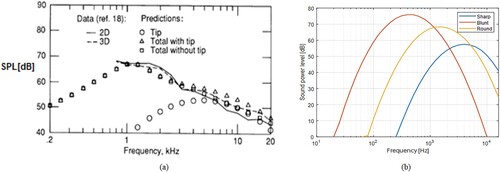
From Figure 9 (a) it can be observed that for the same flow conditions using NACA0012 aerofoil, BPM model prediction deviates significantly at low frequencies when predicting the far field one-third octave sound spectra compared to 2D and 3D experiment data. However, for high-frequency region both BPM and experiment data for trailing edge noise model agree well with each other. This is because the BPM model assumes lower values for turbulence length scale in spanwise direction compared to chord wise direction of aerofoil which influences the suction side boundary layer thickness at the trailing edge due to presence of strong adverse pressure gradients. At 10° AOA, it can be observed that overall noise level for high frequencies shows 2 dB higher due to inclusion of tip noise which was computed at chord length of 12 cm. Hence, a reduction factor was applied on the measured SPL data for trailing edge noise obttained using the original chord length of aerofoil tested in the wind tunnel (Bhargava, Samala, and Anumula 2019; Dijkstra 2015; Leloudas 2006; Moreau, Brooks, and Doolan 2011). Figure 9 (b) shows the effect of tip shape on the tip noise predicted by BPM model. The peak noise predicted by round tip shape is 5-8 dB less than compared to noise level from blunt tip shape. It can be seen that noise peaks for blunt, round and sharp tips appear at frequencies, f ~ 700Hz, f ~ 1kHz and ~ 5kHz respectively in sound spectra. This suggests that for a given mean flow velocity, turbulence field and vortex strength near the tip varies with tip shape that tends to shift the noise peaks towards higher frequencies in sound spectra.

Figure 9. (a) One-third octave band frequency spectra of overall sound pressure level (with and without tip noise contribution) from NACA 0012 airfoil using BPM method having a chord length of 16cm and validated with 2D and 3D experiment wind tunnel data at U = 71.3 m/s and Angle of attack, α = 10° (Brooks, Pope, and Marcolini 1989). (b) Computed tip noise predicted from BPM model for square, round and sharp tip geometries for a 2MW wind turbine blade.

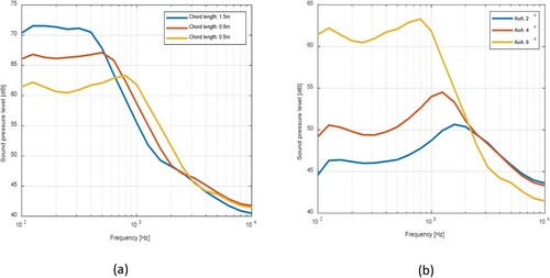
Figure 10(a) shows the overall TBL trailing edge noise for NACA 0012 aerofoils for increase in chord length at constant free stream velocity of 65 m/s. With increase in chord length, the amplitude of noise levels rises by 5 dB in low-frequency region, f ∼ 100 Hz in SPL spectra while no significant difference in noise level is observed for f > 1 kHz in SPL spectra. The computed SPL also included the separation stall noise given by Equation (8) in Section 2.2.1. In wind turbine blades, stall phenomenon is known to occur on blade span in an unsteady manner due to changing blade pitch conditions and operating states of turbine. Stall-regulated wind turbines also use this phenomenon to control the power output from wind turbines. When the flow separation occurs on blade boundary layer due to adverse pressure gradients the stall separation noise component additionally contributes to 5–10 dB to overall peak SPL depending on the mean flow velocity (Brooks, Pope, and Marcolini 1989; Bhargava, Samala, and Anumula 2019; Bhargava and Samala 2019b). Figure 10(b) shows the SPL computed for the NACA 0012 aerofoil at different angles of attack. With increase in angle of attack from 2° to 8° the amplitude of SPL can be found to shift to high-frequency region and exhibits a narrowband peak at f ∼ 1 kHz in SPL spectra. This trend agrees closely with experimental far-field noise data depicted in Figure 9. Further, as high Reynolds number flows on blades of wind turbines are possible, the SPL can be subjected to vary with Reynolds number as well. This is substantiated by Moreau, Roger, and Christophe (2009) who studied stall phenomenon influence on far-field noise spectra using both symmetric and cambered aerofoils. They found that SPL spectra for light and deep stall phenomenon for NACA 0012 aerofoils of chord length below 10 cm and span length below 30 cm exhibited tonal peaks in low-frequency regions of spectrum. Further, an analytical model was proposed for low frequencies based on Curle’s analogy discussed in section 1.2. It was found that light stall produced a low-frequency peak whereas the deep stall vortex shedding from trailing edge produced two peaks in both low and high-frequency regions. For large span widths, low-frequency peaks were significantly higher in amplitude compared to high-frequency peaks, however, as the aerofoil span widths are reduced, the low frequencies spikes are found closely spaced in noise spectrum.

Figure 10. Self-noise spectra turbulent boundary layer trailing edge noise of NACA 0012 computed using BPM method at free stream velocity, U = 65 m/s (a) at 8° AOA for chord lengths of 1.5, 0.8 and 0.5 m (b) for chord length of 0.5 m at 2°, 4° and 8° angle of attack (Bhargava and Samala 2019b; Bhargava and Samala 2019a; Bhargava, Samala, and Anumula 2019).

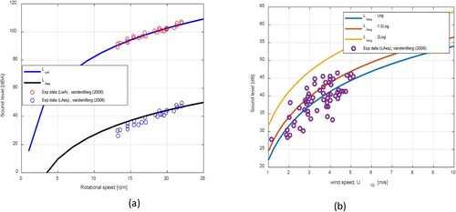
In an experiment study by Van den Berg (2006), it was found that sound levels from wind farms for different microphone configurations were influenced by atmospheric stability patterns during nighttime and daytimes which is one of key determinants of hub height velocity profiles as well as fundamental nature of wind turbine noise. Further, it explains the beating nature of sound termed as swish to help understand the behaviour of wind turbine noise influenced by atmospheric stability patterns. An investigation based on turbine design parameters such as tilt angle was also done to correlate with sound pressure levels. An empirical relationship between microphone screen diameter, mean wind velocity and atmospheric parameters was derived to quantify measurement errors for sound pressure due to presence of microphone screen. The measured sound pressure level was also verified for different atmospheric stability conditions. Figure 11(a,b) shows that L_wA and L_Aeq sound levels from a three-bladed turbine for varying rotational speed and wind speeds agreed well with experiment data. The sound levels were estimated based on Equation (4.4) given in Van den Berg (2006) which demonstrates a difference of 57.9 dBA between L_Aeq and L_wA . Additionally, it can be noted that L_Aeq sound levels predicted using standard U₁₀ and 20% higher U₁₀ logarithmic velocity profile agree within 5% of experiment data compared to 100% rise in U₁₀ velocity profile (Van den Berg 2006).

Figure 11. Comparison of (a) sound pressure (L_Aeq) and power (L_w) level difference with experiment data of Van den Berg (2006) for different rotational speeds of three-bladed turbine (b) sound pressure (L_Aeq) predicted using 1x, 1.2x and 2x logarithmic velocity profile expressions for different wind speeds measured at 10 m height with experiment data of Van den Berg (2006).

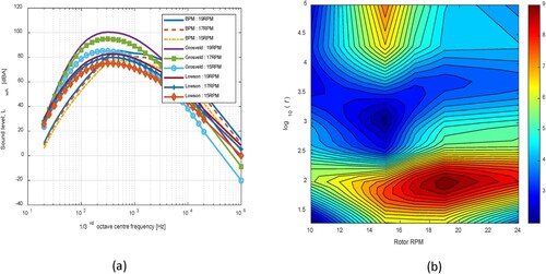
Figure 12(a) shows a comparison of turbulent boundary layer trailing edge noise computed for a wind turbine of blade length of 37 m using BPM, Grosveld and Lowson methods described in Sections 2.2.1–2.2.3. The effect of rotor RPM on the sound power level predicted from these models showed a difference of 3 dBA in the low-frequency region and ∼2 dBA in high-frequency region. Figure 12(b) shows the standard error for SPL predicted by BPM, Grosveld and Lowson models at different rotational speeds of rotor. It can be observed that maximum standard error, 9 dBA is found for f ∼ 100 Hz at 20 RPM. With increasing RPM the standard error is found to reduce up to 3 dBA at 1 kHz. Hence, it can be inferred that rotational speed of rotor strongly influences the overall trailing edge noise level from wind turbines.

Figure 12. (a) Turbulent boundary layer trailing edge noise computed using BPM, Lowson and Grosveld methods as function of rotor RPM (Bhargava and Samala 2019a). (b) Standard error of sound pressure (dBA) between BPM, Lowson and Grosveld methods at U = 8 m/s for increasing rotational speed in RPM.

4. Conclusions

• In this paper, a review of aero-acoustic noise production from airfoils and wind turbine blades shows that predominant acoustic phenomenon such as frequency, pressure intensity, directionality can be adequately predicted by semi-empirical models developed using wind tunnel experiments data. These models can predict sound field fairly accurately when the flow field conditions are within incompressible subsonic range. Past research suggests that CFD-based CAA models predict highly accurate acoustic field compared to analytical and quasi-empirical models. Such models have been extended and improved in several research studies to determine the noise characteristics for different flow conditions.

• Quasi -empirical models have been developed using extensive experimental database and successfully applied for turbulent inflow, trailing edge and tip noise predictions. For wind turbines, operating in a large array amplitude modulation is a major phenomenon that affects noise emission characteristics from rotating blades. An impulsive type noise source is produced from leading edge at infrasonic or low frequencies while swish persists as broadband trailing edge noise source at high frequencies, both of which can be studied to a greater detail.

• Most experimental campaigns conducted on wind turbine noise emissions found that predominant noise occurred from the outer third of blade length during downward motion. Rotational harmonics from a wind turbine vary with blade passing frequencies and produce peak amplitudes at low frequencies but are found to attenuate as the harmonics are increased.

• Finally, passive noise control methods investigated in the past showed that geometric parameters such as aerofoil thickness, serrations on aerofoil structure, span length have the potential for noise reduction up to 20 dB. Optimisation methods in design of low-noise aerofoil profiles, effects of angle of attack, rotational speed, boundary layer turbulence also offer noise reduction potential up to 15 dB.

References

- Arbey, H., and J. Bataille. 1983. “Noise Generated by Airfoils Placed in Uniform Laminar Flow.” Journal of Fluid Mechanics 134: 33–47. doi:10.1017/S0022112083003201.
- Bastasch, M., J. van Dam, B. Sondergaard, and A. Rogers. 2006. “Wind Turbine Noise – An Overview.” Journal of Canadian Acoustical Association 34 (2): 7–16.
- Bhargava, V., S. Maddula, and R. Samala. 2019. “Prediction of Vortex Induced Aerodynamic Noise from Wind Turbine Blades.” Advances in Military Technology, doi:10.3849/aimt.01295.
- Bhargava, V., and R. Samala. 2019a. “Acoustic Emissions from Wind Turbine Blades.” Journal of Aerospace Technology and Management. doi:10.5028/jatm.v11.1071.
- Bhargava, V., and R. Samala. 2019b. “Effect of Boundary Layer on Broadband Noise from Wind Turbine Blades.” Journal of Aerospace Technology and Management, doi:10.5028/jatm.v11.1045.
- Bhargava, V., R. Samala, and C. Anumula. 2019. “Prediction of Broadband Noise from Symmetric and Cambered Airfoils.” INCAS Bulletin, doi:10.13111/2066-8201.2019.11.1.3.
- Blandeau, V.P., and P.F. Joseph. 2011. “Validity of Amiet’s Model for Propeller Trailing Edge Noise.” AIAA Journal 49 (5): 1057–1066. doi:10.2514/1.J050765.
- Brooks, T.F., and T.H. Hodgson. 1981. “Trailing Edge Noise Prediction from Measured Surface Pressures.” Journal of Sound and Vibration 78 (1): 69–117. doi:10.1016/S0022-460X(81)80158-7.
- Brooks, T.F., D.S. Pope, and M.A. Marcolini. 1989. Airfoil Self Noise and Prediction. NASA Reference Publication 1218. https://ntrs.nasa.gov/archive/nasa/casi.ntrs.nasa.gov/19890016302.pdf.
- Buck, S., S. Oerlemans, and S. Palo. 2018. “Experimental Validation of Wind Turbine Inflow Noise Prediction Code, Vol 56, Issue 4.” 22nd AIAA/CEAS Aeroacoustics Conference, Lyon, France.
- Caprio, A.R., F. Avallone, D. Ragni, M. Snellen, and S. van der Zwaag. 2020. “Quantitative Criteria to Design Optimal Permeable Trailing Edges for Noise Abatement.” Journal of Sound and Vibration 485. doi:10.1016/j.jsv.2020.115596.
- Cooper, S. 2021. “Wind Farm Noise – Modulation of the Amplitude.” Acoustics, 364–390. doi:10.3390/acoustics3020025.
- Cotte, B., and Y. Tian. 2016. “Wind Turbine Noise Modeling Based on Amiet’s Theory: Effects of Wind Shear and Atmospheric Turbulence.” Acta Acustica United with Acustica 102: 626–639. doi:10.3813/AAA.918979.
- Curle, N. 1955. “The Influence of Solid Boundaries upon Aerodynamic Sound.” Proceedings of the royal society of London 231: 505–514.
- Dijkstra, P. 2015. “Rotor Noise and Aero-Acoustic Optimization of Wind Turbine Aerofoils.” Master thesis, Department of Aerospace Engineering, Delft University of Technology, 131.
- Doolan, C., D.J. Moreau, E. Arcondoulis, and C. Albarracin. 2012. “Trailing Edge Noise Production, Prediction and Control.” New Zealand Acoustics 25 (3): 22–29.
- Ferziger, J.H., and M. Peric. 1998. Computational Methods for Fluid Dynamics. 3rd ed. Heidelberg: Springer Publishers.
- Ffowcs Williams, J.E., and D.L. Hawkings. 1969. “Sound Generation by Turbulence and Surfaces in Arbitrary Motion.” Philosophical Transactions of the Royal Society of London. Series A, Mathematical and Physical Sciences 264: 321–342.
- Fink, M.R. 1979. Noise Component Method for Airframe Noise.” Journal of Aircraft 16: 659–665. doi:10.2514/3.58586.
- Geyer, T., E. Sarradj, and C. Fritzsche. 2010. “Porous Aerofoils: Noise Reduction and Boundary Layer Effects.” International Journal of Aeroacoustics 9 (6): 787–820. doi:10.1260/1475-472X.9.6.787.
- Goldstein, M.E. 2003. “A Generalized Acoustic Analogy.” Journal of Fluid Mechanics, 315–333. doi:10.1017/S0022112003004890.
- Grosveld, F.W. 1985. “Prediction of Broadband Noise from Horizontal Axis Wind Turbines.” Journal of Propulsion and Power 1 (4): 292–299. ISSN 0748-4658. doi:10.2514/3.22796.
- Hansen, K.L. 2012. “Effect of Leading Edge Tubercles on Airfoil Performance.” Doctor thesis, School of Mechanical Engineering, The University of Adelaide.
- Hansen, K., N. Henrys, C. Hansen, C. Doolan, and D. Moreau. 2012. “Wind Farm Noise – What is a Reasonable Limit in Rural Areas?” Proceedings of Acoustics 2012 – Fremantle, Australia.
- Howe, M.S. 2003. Theory of Vortex Sound. Cambridge University Press. doi:10.1017/CBO9780511755491.
- Hubbard, H.H., and K.P. Shephard. 1991. “Aeroacoustics of Large Wind Turbines.” Journal of Acoustical Society of America 89 (6): 2495–2508. doi:10.1121/1.401021.
- Ikeda, T., S. Enomoto, K. Yamamoto, and K. Amemiya. 2013. “On the Modification of the Ffowcs Williams-Hawkings Integration for Jet Noise Prediction.” Paper Presented at the 19th AIAA/CEAS Aeroacoustics Conference, AIAA 2013-2277, Berlin, May 27–29.
- Kingan, K.M. 2005. “Aero-Acoustic Noise Produced by an Aerofoil.” Doctoral thesis, University of Canterbury, New Zealand, 448. https://ir.canterbury.ac.nz/handle/10092/6596.
- Kingan, M.J., and J.R. Pearse. 2009. “Laminar Boundary Layer Instability Noise Produced by an Aerofoil.” Journal of Sound and Vibration 322: 808–828. doi:10.1016/j.jsv.2008.11.043.
- Leloudas, G. 2006. “Optimization of Wind Turbines with Respect to Noise.” Master thesis, Technical University of Denmark, Lyngby, 66. http://outer.space.dtu.dk/~giorgos/images/giorgiosleloudas2006.pdf.
- Li, F., Q. Huang, G. Pan, and Y. Shi. 2021. “Numerical Study on Hydrodynamic Performance and Flow Noise of a Hydrofoil with Wavy Leading-Edge.” AIP Advances 11 (9): 095105. doi:10.1063/5.0064343.
- Li, T., D. Qin, N. Zhou, and W. Zhang. 2022. “Step-by-Step Numerical Prediction of Aerodynamic Noise Generated by High Speed Trains.” Chinese Journal of Mechanical Engineering 35 (1): 549. doi:10.1186/s10033-022-00705-4.
- Lighthill, M.J., and M.H.A. Newman. 1952. “On Sound Generated Aerodynamically. General Theory.” Proceedings of the Royal Society of London. Series A. Mathematical and Physical Sciences 211 (1107): 564–587.
- Lowson, M.V. 1970. “Theoretical Analysis of Compressor Noise.” Journal of Acoustical Society of America 47 (1): 371–385. doi:10.1121/1.1911508.
- Lowson, M.V. 1992. Assessment and Prediction of Wind Turbine Noise, Flow Solutions Report 92/19, STSU W/13/00284/REP, Bristol, England.
- McAlpine, A., E.C. Nash, and M.V. Lowson. 1999. “On the Generation of Discrete Frequency Tones by the Flow Around an Airfoil.” Journal of Sound and Vibration 222: 753–779. doi:10.1006/jsvi.1998.2085.
- Moreau, D. 2021. “Flow Induced Noise Regimes for Three-Dimensional Airfoil.” Proceedings of Acoustics 2021, Wollongong, NSW, Australia.
- Moreau, D.J., L.A. Brooks, and C. Doolan. 2011. “Flat Plate Self-Noise Reduction at Low to Moderate Reynolds Number with Trailing Edge Serrations.” Proceedings of Acoustics, Gold Coast, Australia. https://pdfs.semanticscholar.org/74fa/0f9f258c0d5c5a1f846abb244c6d7505b213.pdf.
- Moreau, S., M. Roger, and J. Christophe. 2009. “Flow Features and Self-Noise of Airfoils Near Stall or in Stall.” 30th AIAA Aeroacoustics Conference. doi:10.2514/6.2009-3198.
- Moriarty, P., and P. Migliore. 2003. “Semi Empirical Aero-Acoustic Noise Prediction Code for Wind Turbines.” Technical Report. http://citeseerx.ist.psu.edu/viewdoc/download?doi=10.1.1.197.1153&rep=rep1&type=pdf.
- Nataraj, P.P. 2022. Airfoil Self Noise Predictions Using DDES and the FW-H Analogy. Department of Mechanical Engineering, University of Twente.
- Oerlemans, S., P. Sijtsma, and M.B. Lopez. 2007. “Location and Quantification of Noise Sources on a Wind Turbine.” Journal of Sound and Vibration 299 (5), doi:10.1016/j.jsv.2006.07.032.
- Paterson, R.W., and R.K. Amiet. 1976. Acoustic Radiation and Surface Pressure Characteristics of an Airfoil due to Incident Turbulence, NASA Report, CR-2733.
- Paterson, R.W., P.G. Vogt, M.R. Fink, and C.L. Munch. 1973. “Vortex Noise of Isolated Airfoils.” Journal of Aircraft 10: 296–302. doi:10.2514/3.60229.
- Poggi, C., M. Rossetti, G. Bernardini, U. Iemma, C. Andolfi, C. Milano, and M. Gennaretti. 2021. “Surrogate Models for Predicting Noise Emission and Aerodynamic Performance of Propellers.” Aerospace Science and Technology (In Press). doi:10.1016/j.ast.2021.107016.
- Pouangué, A.F., M. Sanjosé, S. Moreau, G. Daviller, and H. Deniau. 2015. “Subsonic Jet Noise Simulations Using Both Structured and Unstructured Grids.” AIAA Journal 53 (1): 55–69. doi:10.2514/1.J052380.
- Powell, A. 1964. “Theory of Vortex Sound.” Journal of Acoustical Society of America 36: 177–195. doi:10.1121/1.1918931.
- Qin, D., T. Li, Z. Dai, and J. Zhang. 2022. “Study on Prediction in Far-Field Aerodynamic Noise of Long-Marshalling High-Speed Train.” Environmental Science and Pollution Research 29 (57): 86580–86594. doi:10.1007/s11356-022-21215-9.
- Sabat, A., C. Daitx, and S. Qi. Integrative Predictive Modelling for Airfoil Self Noise.
- Schlinker, R., and R.K. Amiet. 1981. “Helicopter Rotor Trailing Edge Noise.” NASA CR 3470.
- Shapiro, P.J. 1977. “The Influence of Sound Upon Laminar Boundary Layer Instability.” Report No: 83458-83560-1.
- Shen, W.Z., W.J. Zhu, E. Barlas, and Y. Li. 2019. “Advanced Flow and Noise Simulation Method for Wind Farm Assessment in Complex Terrain.” Renewable Energy, doi:10.1016/j.renene.2019.05.140.
- Shur, M.L., P.R. Spalart, M.K. Strelets, and A.K. Travin. 2003. “Towards the Prediction of Noise from jet Engines.” International Journal of Heat and Fluid Flow 24 (4): 551–561. doi:10.1016/S0142-727X(03)00049-3.
- Tam, C.K.W. 1974. “Discrete Tones of Isolated Airfoils.” Journal of Acoustical Society of America 55: 1173–1177. doi:10.1121/1.1914682.
- Tang, H., Y. Lei, and Y. Fu. 2019. “Noise Reduction Mechanisms of an Airfoil with Trailing Edge Serrations at low Mach Number.” Applied Science, MDPI, doi:10.3390/app9183784.
- Van den Berg, G.P. 2006. “The Sound of High Winds: The Effect of Atmospheric Stability on Wind Turbine Sound and Microphone Noise.” Doctoral thesis, University of Groningen.
- Viterna, L.A. 1981. “The NASA LeRC Wind Turbine Sound Prediction Code, 2nd DOE/NASA Wind Turbine Dynamics Workshop.” Report no: TM-81737/20366-1.
- Wagner, C., T. Hüttl, and P. Sagaut, eds. 2007. “Introduction.” In Cambridge Aerospace Series, 1–23. London: Cambridge University Press.
- Wei, Z.J., W.Z. Shen, J.N. Sorensen, and G. Leloudas. 2016. “Improvement of Airfoil Trailing Edge Bluntness Noise Model.” Advances in Mechanical Engineering 8 (2): 1–12. doi:10.1177/1687814016629343.
- Wolf, W.R., J.L. Azevedo, and S.K. Lele. 2012. Effects of Mean Flow Convection and Quadrupole Sources on Airfoil Trailing Edge Noise.
- Wolf, W.R., J.G. Kocheemoolayil, and S.K. Lele. 2014. “Large Eddy Simulation of Stall Noise.” 20th AIAA/CEAS Aeroacoustics Conference. doi:10.2514/6.2014-3182.
- Yao, H.-D., L. Davidson, and L.-E. Eriksson. 2017. “Noise Radiated by Low-Reynolds Number Flows Past a Hemisphere at Ma = 0.3.” Physics of Fluids 29 (7): 076102. doi:10.1063/1.4994592.
- Zhang, Y., F. Avallone, and S. Watson. 2022. “An Aero-Acoustic Based Approach for Wind Turbine Blade Damage Detection, The Science of Making Torque from Wind (TORQUE, 2022).” Journal of Physics Conference Series. IOP Publishing. doi:10.1088/1742-6596/2265/2/022088.
- Zhou, Z., Z. Zang, H. Wang, and S. Wang. 2022. “Far Field Approximations to the Derivative of Greens Function for the Ffowcs Williams and Hawkings Equation.” Advances in Aerodynamics. doi:10.1186/s42774-022-00109-x.
- Zhu, W.J. 2004. “Modeling of Noise from Wind Turbines.” Master thesis, Department of Wind Energy, Technical University of Denmark, Lyngby.
- Zhu, W.J., Wen Zhong Shen, and J.N. Sorensen. 2016. “Low Noise Airfoil and Turbine Design.” In Wind Turbines-Design, Control and Applications, 55–72. Intech Open. doi:10.5772/63335.
- Zidan, E., T. Elnady, and A. Elsabbagh. 2014. “Comparison of Sound Power Prediction Models of Wind Turbines, International Conference on Advances in Agricultural.” Biological & Environmental Sciences (AABES-2014). doi:10.15242/IICBE.C1014154.