Energy loss comparison between kinematically equivalent mechanisms: Slider-crank and eccentric cam

Abstract

The reduction of energy consumption in industrial processes is a challenge to be confronted within the framework of the United Nations’ Sustainable Development Goals. The present study compares the energy loss per cycle of two kinematically equivalent mechanisms: a slider-crank and an eccentric cam with a translational roller follower. We use the work-energy theorem to evaluate energy losses by using a viscous friction model in a stationary regime. The innovation of this study lies in the energetic comparison to identify the best and worst alternatives by analyzing the contribution of their main geometrical parameters, such as crank length, rod-crank length ratio, roller radius and follower offset. The aim is to provide guidelines to help machinery designers to take relevant preliminary decisions that affect energy efficiency. Herein, we include analytical models, numerical simulations and experimental results using a test stand that can be adapted to other planar one degree-of-freedom mechanisms. In this context, we conclude that an eccentric cam mechanism with a big roller radius and no offset provides the best energetic efficiency among the aforementioned mechanisms.

Keywords:

• Energy loss comparison
• cam mechanism
• slider-crank mechanism
• experimental mechanics

1. Introduction

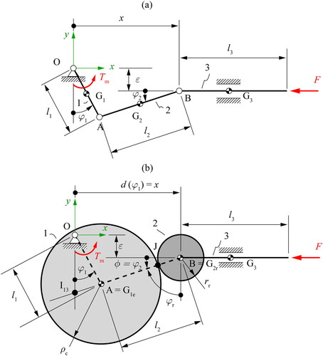
The slider-crank mechanism (Fig. 1(a)) and the eccentric cam mechanism (Fig. 1(b)) are planar one degree-of-freedom mechanical transmission systems used to transform a full rotational input motion into a translational output motion. Both mechanisms are kinematically equivalent (Cardona and Clos 2009; Norton 2002; Rothbart 2003) and are common solutions in automated production machinery. The existing design guidelines (Norton 2002) state that a cam mechanism is more difficult and expensive to manufacture than an equivalent linkage mechanism. However, a cam mechanism can be more compact and easier to design for a specific output motion, and may be the only possible solution if, for example, the crank length is so small that it physically prevents the installation of two revolute pairs.

Figure 1. (a) Slider-crank mechanism; (b) Eccentric cam mechanism.

Pabiszczak and Kowal (2022) studied the energetic efficiency of an eccentric rolling transmission (ERT) as an alternative to a gear transmission. As a function generator, Ottaviano et al. (2008) compared a cam transmission with a noncircular gear coupled with a slider-crank mechanism. For circular-arc cams, acceleration, and torque analysis has been carried out as well (Lanni, Carbone, et al. 2006; Lanni, Ceccarelli and Cajun, 2006).

Even though previous authors have compared several mechanisms, there are few available studies that focus on energy loss or efficiency evaluation, despite being an issue that is gaining relevance in machinery design. Freudenstein, Mayourian, and Maki (1983) proposed a coefficient to evaluate the energy loss in cam mechanisms with flat-faced followers for force-closed and form-closed systems; they studied several basic cam curves and compared the values for this coefficient. Yau and Longman (2011) assessed the potential of reducing energy usage in a force-closed cam mechanism using variable pitch springs between the coils. For the specific case of an ERT, Pabiszczak and Kowal (2022) calculated its efficiency and validated it experimentally using torque meters on the input and output shafts. Yang et al. (2022) proposed a new nonlinear variable stiffness actuator (VSA) by using an eccentric cam mechanism with a translational roller follower against a variable-in-length leaf spring. They achieve a low-energy consumption VSA design that eliminates sliding friction in some pairs using a combination of rollers and rollers bearings.

Energy losses are related to friction. The quantification of friction between two solids is a complex problem, especially from a tribological perspective (Alakhramsing et al. 2018a, 2018b, 2019). There is plenty of scientific literature dealing with different friction force models. For example, Pennestrì et al. (2016) presented a review and numerical efficiency comparison of eight widespread friction models and Marques et al. (2016) reviewed 21 well-known different friction force models.

Several authors have applied Coulomb friction models to the translational lower pair that exists in the slider or follower link (Freudenstein, Mayourian, and Maki 1983; Norton 2002; Rothbart 2003; Wu et al. 2009). Other authors have applied viscous friction coefficients to cam mechanisms (Català et al. 2016; Ouyang et al. 2017) or in a rolling device based on a five-bar linkage mechanism (Yu et al. 2022). Moreover, at the cam-roller contact, other authors have applied a combination of Coulomb and viscous friction models (De Groote et al. 2022) and elastohydrodynamic lubrication (EHL) models (Català et al. 2013; Alakhramsing et al. 2018b). Bai et al. (2022) studied a planar slider-crank mechanism assuming axial and radial dimensional clearances by using a modified Coulomb friction model that considers a sliding friction coefficient.

Experimental validations of dry friction, viscous friction and rolling resistance coefficients are reported in several works (De Groote et al. 2022; Li, Cheng, and Xie 2019; Li, Cheng, and Xie 2019).

The present article compares the energy losses between two competitive solutions: a slider-crank mechanism and an eccentric cam mechanism with a translational roller follower. For each mechanism, we quantify the energy that is lost per cycle at the lower pairs by applying viscous friction models in a stationary regime, while assuming ideal kinematic pairs with no clearances and well-lubricated. Hence, only the kinematic solution is necessary, allowing for an immediate study to detect energy efficiency trends over a large range of dimensions of the main geometrical parameters: crank length, rod-crank length ratio, roller radius, and follower offset.

Nevertheless, for the higher pair between the eccentric cam and the roller, energy loss due to elastic deformation is evaluated using the mixed-elastohydrodynamic friction model based on Masjedi and Khonsari (2015). Additionally, vector theorems have been solved for both mechanisms to allow the dynamic comparison transmission efficiency of force. Despite the fact that the highest Hertz pressures are located at the contact between the eccentric cam and the roller (finite contact line), we prove that energy loss is negligible for the case study and assume no sliding, as done by Sanmiguel-Rojas and Hidalgo-Martínez (2016). Next, we assume that energy loss due to elastic deformations in the lower pairs with contact surface areas can be also neglected, as carried out by Alakhramsing et al. (2018a, 2018b, 2019).

The innovations we present herein are: (i) the evaluation of the influence of the main geometric parameters in terms of the total energy losses to identify the best alternative among the kinematically equivalent mechanisms; and (ii) the validation of the trends in terms of energy losses (the best and worst options) using a test stand, which can be adapted to other planar one degree-of-freedom mechanisms, or to experimentally evaluate energy losses predicted for other friction models.

This article is organized as follows. In Section 2, we state the problem formulation. In Section 3, we first develop a numerical example and then describe our chosen assumptions in order to compare them in terms of the total energy loss per cycle. The results of this comparison are depicted for a range of scales of their main geometrical parameters. We present our experimental results in Section 4, and finally, we outline our conclusions in Section 5.

2. Problem formulation

2.1. Slider-crank mechanism formulation

A slider-crank mechanism (Fig. 1(a)) has four lower pairs with three movable links: a crank (1)(1) $$l_1\hspace{0.17em}\mathrm{\text{sin}}\hspace{0.17em}{\phi }_1+l_2\hspace{0.17em}\mathrm{\text{cos}}\hspace{0.17em}{\phi }_2-x=0$$(1) , a rod (2)(2) $$-l_1\hspace{0.17em}\mathrm{\text{cos}}\hspace{0.17em}{\phi }_1+l_2\hspace{0.17em}\mathrm{\text{sin}}\hspace{0.17em}{\phi }_2+\epsilon =0$$(2) and a slider (3)(3) $${\dot{\phi }}_2=-\frac{l_1\hspace{0.17em}\mathrm{\text{sin}}\hspace{0.17em}{\phi }_1}{l_2\hspace{0.17em}\mathrm{\text{cos}}\hspace{0.17em}{\phi }_2}{\dot{\phi }}_1$$(3) .

According to Fig. 1(a), all possible configurations, velocities, and accelerations of the mechanism are described by generalized coordinates $\mathit{q}={\left\{{\phi }_1,{\phi }_2,x\right\}}^{\mathrm{T}}$ and the first and second temporal derivatives, $\dot{\mathit{q}}={\left\{{\dot{\phi }}_1,{\dot{\phi }}_2,\dot{x}\right\}}^{\mathrm{T}}$ and $\ddot{\mathit{q}}={\left\{{\ddot{\phi }}_1,{\ddot{\phi }}_2,\ddot{x}\right\}}^{\mathrm{T}},$ respectively. The independent coordinate is ${\phi }_1.$ By applying the closed loop method, we obtain two constraint equations, as presented in Eqs. (1)(1) $$l_1\hspace{0.17em}\mathrm{\text{sin}}\hspace{0.17em}{\phi }_1+l_2\hspace{0.17em}\mathrm{\text{cos}}\hspace{0.17em}{\phi }_2-x=0$$(1) and (2)(2) $$-l_1\hspace{0.17em}\mathrm{\text{cos}}\hspace{0.17em}{\phi }_1+l_2\hspace{0.17em}\mathrm{\text{sin}}\hspace{0.17em}{\phi }_2+\epsilon =0$$(2) . (1) $$l_1\hspace{0.17em}\mathrm{\text{sin}}\hspace{0.17em}{\phi }_1+l_2\hspace{0.17em}\mathrm{\text{cos}}\hspace{0.17em}{\phi }_2-x=0$$(1) (2) $$-l_1\hspace{0.17em}\mathrm{\text{cos}}\hspace{0.17em}{\phi }_1+l_2\hspace{0.17em}\mathrm{\text{sin}}\hspace{0.17em}{\phi }_2+\epsilon =0$$(2)

The velocities $\dot{\mathit{q}}$ of the mechanism are obtained with the first temporal derivative of Eqs. (1)(1) $$l_1\hspace{0.17em}\mathrm{\text{sin}}\hspace{0.17em}{\phi }_1+l_2\hspace{0.17em}\mathrm{\text{cos}}\hspace{0.17em}{\phi }_2-x=0$$(1) and (2)(2) $$-l_1\hspace{0.17em}\mathrm{\text{cos}}\hspace{0.17em}{\phi }_1+l_2\hspace{0.17em}\mathrm{\text{sin}}\hspace{0.17em}{\phi }_2+\epsilon =0$$(2) . Rearranging the terms, Eqs. (3)(3) $${\dot{\phi }}_2=-\frac{l_1\hspace{0.17em}\mathrm{\text{sin}}\hspace{0.17em}{\phi }_1}{l_2\hspace{0.17em}\mathrm{\text{cos}}\hspace{0.17em}{\phi }_2}{\dot{\phi }}_1$$(3) and (4)(4) $$\dot{x}=l_1\frac{\hspace{0.17em}\mathrm{\text{cos}}\hspace{0.17em}\left({\phi }_1-{\phi }_2\right)}{\hspace{0.17em}\mathrm{\text{cos}}\hspace{0.17em}{\phi }_2}{\dot{\phi }}_1$$(4) are obtained to show the dependent velocities ${\dot{\phi }}_2$ and $\dot{x}$ as a function of the independent angular velocity ${\dot{\phi }}_1.$ (3) $${\dot{\phi }}_2=-\frac{l_1\hspace{0.17em}\mathrm{\text{sin}}\hspace{0.17em}{\phi }_1}{l_2\hspace{0.17em}\mathrm{\text{cos}}\hspace{0.17em}{\phi }_2}{\dot{\phi }}_1$$(3) (4) $$\dot{x}=l_1\frac{\hspace{0.17em}\mathrm{\text{cos}}\hspace{0.17em}\left({\phi }_1-{\phi }_2\right)}{\hspace{0.17em}\mathrm{\text{cos}}\hspace{0.17em}{\phi }_2}{\dot{\phi }}_1$$(4)

Figure 2 shows the Free Body Diagram (FBD) for the three links of the slider-crank mechanism. The parameters required for the dynamic simulations are explained in Table 1.

Figure 2. FBD for each link of a slider-crank mechanism.

Table 1. Dynamic variables and parameters for the slider-crank mechanism.

Parameter	Description
$T_{\mathrm{m}}$	Motor torque
$R_{x\mathrm{O}},$ $R_{y\mathrm{O}},$ $R_{x\mathrm{A}},$ $R_{y\mathrm{A}},$ $R_{x\mathrm{B}}$ and $R_{y\mathrm{B}}$	Internal reaction forces in the revolute pairs O, A and B, respectively
$N_3$ and $M_3$	Internal reaction normal force and moment in the prismatic pair, respectively
$T_{\mathrm{O}},$ $T_{\mathrm{A}}$ and $T_{\mathrm{B}}$	Friction torques in the revolute pairs O, A and B, respectively
$c_{\mathrm{O}},$ $c_{\mathrm{A}}$ and $c_{\mathrm{B}}$	Viscous friction coefficients in the revolute pairs O, A and B, respectively
$F_3$	Friction force in the prismatic pair
$c_3$	Viscous friction coefficient between the slider and the fixed guide
$F$	External force
$m_1,$ $m_2$ and $m_3$	Mass of the crank, the rod and the slider, respectively
$I_{{\mathrm{G}}_1}$	Crank moment of inertia along the z-axis referring to its center of inertia (${\mathrm{G}}_1$)
$I_{{\mathrm{G}}_2}$	Rod moment of inertia along the z-axis referring to its center of inertia (${\mathrm{G}}_2$)

Equations (5–13) are obtained using vector theorems for each movable link of the mechanism. (5) $$R_{x\mathrm{O}}+R_{x\mathrm{A}}=m_1\left({\ddot{\phi }}_1\frac{l_1}{2}\mathrm{\text{cos}}\hspace{0.17em}{\phi }_1-{\dot{\phi }}_1^2\frac{l_1}{2}\mathrm{\text{sin}}\hspace{0.17em}{\phi }_1\right)$$(5) (6) $$R_{\mathit{\text{yO}}}+R_{y\mathrm{A}}=m_1\left({\ddot{\phi }}_1\frac{l_1}{2}\mathrm{\text{sin}}\hspace{0.17em}{\phi }_1+{\dot{\phi }}_1^2\frac{l_1}{2}\mathrm{\text{cos}}\hspace{0.17em}{\phi }_1\right)$$(6) (7) $$T_{\mathrm{m}}-T_{\mathrm{O}}-T_{\mathrm{A}}+\frac{l_1}{2}\left(\left(R_{x\mathrm{A}}-R_{x\mathrm{O}}\right)\hspace{0.17em}\mathrm{\text{cos}}\hspace{0.17em}{\phi }_1+\left(R_{y\mathrm{A}}-R_{y\mathrm{O}}\right)\hspace{0.17em}\mathrm{\text{sin}}\hspace{0.17em}{\phi }_1\right)=I_{{\mathrm{G}}_1}{\ddot{\phi }}_1$$(7) (8) $$-R_{x\mathrm{A}}+R_{x\mathrm{B}}=m_2\left({\ddot{\phi }}_1{l}_1\hspace{0.17em}\mathrm{\text{cos}}\hspace{0.17em}{\phi }_1-{\dot{\phi }}_1^2{l}_1\hspace{0.17em}\mathrm{\text{sin}}\hspace{0.17em}{\phi }_1-{\ddot{\phi }}_2\frac{l_2}{2}\mathrm{\text{sin}}\hspace{0.17em}{\phi }_2-{\dot{\phi }}_2^2\frac{l_2}{2}\mathrm{\text{cos}}\hspace{0.17em}{\phi }_2\right)$$(8) (9) $$-R_{y\mathrm{A}}+R_{y\mathrm{B}}=m_2\left({\ddot{\phi }}_1{l}_1\hspace{0.17em}\mathrm{\text{sin}}\hspace{0.17em}{\phi }_1+{\dot{\phi }}_1^2{l}_1\hspace{0.17em}\mathrm{\text{cos}}\hspace{0.17em}{\phi }_1+{\ddot{\phi }}_2\frac{l_2}{2}\mathrm{\text{cos}}\hspace{0.17em}{\phi }_2-{\dot{\phi }}_2^2\frac{l_2}{2}\mathrm{\text{sin}}\hspace{0.17em}{\phi }_2\right)$$(9) (10) $$T_{\mathrm{A}}-T_{\mathrm{B}}+\frac{l_2}{2}\left(\left(-R_{x\mathrm{A}}-R_{x\mathrm{B}}\right)\hspace{0.17em}\mathrm{\text{sin}}\hspace{0.17em}{\phi }_2+\left(R_{y\mathrm{A}}+R_{y\mathrm{B}}\right)\hspace{0.17em}\mathrm{\text{cos}}\hspace{0.17em}{\phi }_2\right)=I_{{\mathrm{G}}_2}{\ddot{\phi }}_2$$(10) (11) $$-R_{x\mathrm{B}}-F_3-F=m_3\ddot{x}$$(11) (12) $$-R_{y\mathrm{B}}+N_3=0$$(12) (13) $$T_{\mathrm{B}}+N_3\frac{l_3}{2}+M_3=0$$(13)

The friction torques $T_{\mathrm{O}},$ $T_{\mathrm{A}},$ $T_{\mathrm{B}}$ and the friction force $F_3$ are calculated with Eqs. (14–17), respectively. (14) $$T_{\mathrm{O}}=c_{\mathrm{O}}{\dot{\phi }}_1$$(14) (15) $$T_{\mathrm{A}}=c_{\mathrm{A}}\left({\dot{\phi }}_1-{\dot{\phi }}_2\right)$$(15) (16) $$T_{\mathrm{B}}=c_{\mathrm{B}}{\dot{\phi }}_2$$(16) (17) $$F_3=c_3\dot{x}$$(17)

Despite not being necessary in a slider-crank mechanism, an external force $F$ (Fig. 1(a)) has been added for comparison purposes with a force-closing eccentric cam mechanism.

The total energy loss $E_{\text{loss}}$ for each cycle is quantified using Eq. (18)(18) $$E_{\text{loss}}=\oint \left({\mathit{T}}_{\mathit{O}}\cdot {\dot{\mathit{\phi }}}_1+{\mathit{T}}_{\mathit{A}}\cdot {\dot{\mathit{\phi }}}_1+{\mathit{T}}_{\mathit{A}}\cdot {\dot{\mathit{\phi }}}_2+{\mathit{T}}_{\mathit{B}}\cdot {\dot{\mathit{\phi }}}_2+{\mathit{F}}_3\cdot \dot{\mathit{x}}\right)\mathrm{d}t$$(18) as the integral of instantaneous power losses, $E_{\text{loss}}=\oint P_{\text{loss}}\mathrm{d}t.$ (18) $$E_{\text{loss}}=\oint \left({\mathit{T}}_{\mathit{O}}\cdot {\dot{\mathit{\phi }}}_1+{\mathit{T}}_{\mathit{A}}\cdot {\dot{\mathit{\phi }}}_1+{\mathit{T}}_{\mathit{A}}\cdot {\dot{\mathit{\phi }}}_2+{\mathit{T}}_{\mathit{B}}\cdot {\dot{\mathit{\phi }}}_2+{\mathit{F}}_3\cdot \dot{\mathit{x}}\right)\mathrm{d}t$$(18)

2.2. Eccentric cam mechanism formulation

An eccentric cam mechanism (Fig. 1(b)) has three lower pairs and one higher pair, and 3 movable links: an eccentric cam (1)(1) $$l_1\hspace{0.17em}\mathrm{\text{sin}}\hspace{0.17em}{\phi }_1+l_2\hspace{0.17em}\mathrm{\text{cos}}\hspace{0.17em}{\phi }_2-x=0$$(1) , a roller (2)(2) $$-l_1\hspace{0.17em}\mathrm{\text{cos}}\hspace{0.17em}{\phi }_1+l_2\hspace{0.17em}\mathrm{\text{sin}}\hspace{0.17em}{\phi }_2+\epsilon =0$$(2) and a follower (3)(3) $${\dot{\phi }}_2=-\frac{l_1\hspace{0.17em}\mathrm{\text{sin}}\hspace{0.17em}{\phi }_1}{l_2\hspace{0.17em}\mathrm{\text{cos}}\hspace{0.17em}{\phi }_2}{\dot{\phi }}_1$$(3) . The geometrical parameters presented in Fig. 1(b) are described in Table 2.

Table 2. Geometric parameters for the eccentric cam mechanism.

Parameter	Description
${\phi }_1$	Eccentric cam angular displacement
${\phi }_{\mathrm{r}}$	Roller angular displacement
$d({\phi }_1)=x({\phi }_1)$	Linear displacement function imposed on the roller center
$\epsilon$	Positive offset between the follower’s motion axis and the rotational center of the eccentric cam
$l_1$	Eccentricity between the rotational center of the eccentric cam and the center of inertia (A = G1e); equivalent crank length
${\rho }_{\mathrm{c}}$	Eccentric cam curvature radius
$l_2$	Equivalent rod length
$r_{\mathrm{r}}$	Roller radius
$\varphi ={\phi }_2$	Pressure angle
$l_3$	Follower length
${\mathrm{I}}_{13}$	Instantaneous rotational center between the eccentric cam (link 1) and the follower (link 3), assuming no sliding at contact

The linear displacement function of the eccentric cam mechanism is equal to the output of the slider-crank mechanism, which means $d({\phi }_1)=x({\phi }_1).$ Considering Eqs (1)(1) $$l_1\hspace{0.17em}\mathrm{\text{sin}}\hspace{0.17em}{\phi }_1+l_2\hspace{0.17em}\mathrm{\text{cos}}\hspace{0.17em}{\phi }_2-x=0$$(1) and (2)(2) $$-l_1\hspace{0.17em}\mathrm{\text{cos}}\hspace{0.17em}{\phi }_1+l_2\hspace{0.17em}\mathrm{\text{sin}}\hspace{0.17em}{\phi }_2+\epsilon =0$$(2) , $d({\phi }_1)$ is defined according to Eq. (19)(19) $$d=l_1\hspace{0.17em}\mathrm{\text{sin}}\hspace{0.17em}{\phi }_1+l_2\hspace{0.17em}\mathrm{\text{cos}}\hspace{0.17em}\left({\text{sin}}^{-1}\left(\frac{l_1\hspace{0.17em}\mathrm{\text{cos}}\hspace{0.17em}{\phi }_1-\epsilon }{l_2}\right)\right)$$(19) . (19) $$d=l_1\hspace{0.17em}\mathrm{\text{sin}}\hspace{0.17em}{\phi }_1+l_2\hspace{0.17em}\mathrm{\text{cos}}\hspace{0.17em}\left({\text{sin}}^{-1}\left(\frac{l_1\hspace{0.17em}\mathrm{\text{cos}}\hspace{0.17em}{\phi }_1-\epsilon }{l_2}\right)\right)$$(19)

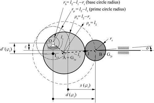
It is common to define $d({\phi }_1)$ using Eq. (20)(20) $$d\left({\phi }_1\right)=s\left({\phi }_1\right)+\sqrt{r_{\mathrm{p}}^2-{\epsilon }^2}$$(20) , where: $s({\phi }_1)$ is a motion law defined with its minimum value equal to zero ($s_{\mathrm{\text{min}}}=0$) and $r_{\mathrm{p}}$ is the prime circle radius. This is shown in Fig. 3 and is calculated according to Eq. (21)(21) $$r_{\mathrm{p}}=r_{\mathrm{b}}+r_{\mathrm{r}}$$(21) after choosing a value for the base circle cam radius $r_{\mathrm{b}},$ and a value for the roller radius $r_{\mathrm{r}}.$ (20) $$d\left({\phi }_1\right)=s\left({\phi }_1\right)+\sqrt{r_{\mathrm{p}}^2-{\epsilon }^2}$$(20) (21) $$r_{\mathrm{p}}=r_{\mathrm{b}}+r_{\mathrm{r}}$$(21)

Figure 3. Geometric parameters for an eccentric cam mechanism.

The motion law is defined as $s({\phi }_1)=x({\phi }_1)-x_{\mathrm{\text{min}}};$ from Fig. 1(a), it is derived that $x_{\mathrm{\text{min}}}=\sqrt{{(l_2-l_1)}^2-{\epsilon }^2}.$ Then $s({\phi }_1)$ is obtained using Eq. (22)(22) $$s\left({\phi }_1\right)=x\left({\phi }_1\right)-\sqrt{{\left(l_2-l_1\right)}^2-{\epsilon }^2}$$(22) (22) $$s\left({\phi }_1\right)=x\left({\phi }_1\right)-\sqrt{{\left(l_2-l_1\right)}^2-{\epsilon }^2}$$(22)

By combining Eq. (20)(20) $$d\left({\phi }_1\right)=s\left({\phi }_1\right)+\sqrt{r_{\mathrm{p}}^2-{\epsilon }^2}$$(20) with (22)(22) $$s\left({\phi }_1\right)=x\left({\phi }_1\right)-\sqrt{{\left(l_2-l_1\right)}^2-{\epsilon }^2}$$(22) and recognizing that $d({\phi }_1)=x({\phi }_1),$ the prime circle radius for an eccentric cam is thus $r_{\mathrm{p}}=l_2-l_1.$

The first and second derivatives of $d({\phi }_1)$ with respect to ${\phi }_1,$ $d^{\prime }({\phi }_1)=\mathrm{d}d/\mathrm{d}{\phi }_1$ and $d^{″}({\phi }_1)={\mathrm{d}}^{2}d/\mathrm{d}{\phi }_1^2,$ using Eq. (19)(19) $$d=l_1\hspace{0.17em}\mathrm{\text{sin}}\hspace{0.17em}{\phi }_1+l_2\hspace{0.17em}\mathrm{\text{cos}}\hspace{0.17em}\left({\text{sin}}^{-1}\left(\frac{l_1\hspace{0.17em}\mathrm{\text{cos}}\hspace{0.17em}{\phi }_1-\epsilon }{l_2}\right)\right)$$(19) are (23) $$d^{\prime }\left({\phi }_1\right)=l_1\left(\hspace{0.17em}\mathrm{\text{cos}}\hspace{0.17em}{\phi }_1+\frac{\left(l_1\hspace{0.17em}\mathrm{\text{cos}}\hspace{0.17em}{\phi }_1-\epsilon \right)\hspace{0.17em}\mathrm{\text{sin}}\hspace{0.17em}{\phi }_1}{l_2\sqrt{1-{\left(\frac{l_1\hspace{0.17em}\mathrm{\text{cos}}\hspace{0.17em}{\phi }_1-\epsilon }{l_2}\right)}^2}}\right)$$(23) (24) $$\begin{array}{l}{d}^{″}\left({\phi }_1\right)=-l_1\hspace{0.17em}\mathrm{\text{sin}}\hspace{0.17em}{\phi }_1\\ +l_1\left(\frac{l_2^2\left(-l_1{\hspace{0.17em}\mathrm{\text{sin}}\hspace{0.17em}}^2{\phi }_1+\left(l_1\hspace{0.17em}\mathrm{\text{cos}}\hspace{0.17em}{\phi }_1-\epsilon \right)\hspace{0.17em}\mathrm{\text{cos}}\hspace{0.17em}{\phi }_1\right)\left(1-{\left(\frac{l_1\hspace{0.17em}\mathrm{\text{cos}}\hspace{0.17em}{\phi }_1-\epsilon }{l_2}\right)}^2\right)-l_1{\hspace{0.17em}\mathrm{\text{sin}}\hspace{0.17em}}^2{\phi }_1{\left(l_1\hspace{0.17em}\mathrm{\text{cos}}\hspace{0.17em}{\phi }_1-\epsilon \right)}^2}{l_2^3\sqrt{{\left(1-{\left(\frac{l_1\hspace{0.17em}\mathrm{\text{cos}}\hspace{0.17em}{\phi }_1-\epsilon }{l_2}\right)}^2\right)}^3}}\right)\end{array}$$(24) In the literature, it has been demonstrated that the distance between point O and ${\mathrm{I}}_{13}$ is equal to $d^{\prime }({\phi }_1)$ (Fig. 3), which only depends on geometric parameters and is independent of the angular velocity of the cam.

The common geometrical indexes to evaluate whether a cam profile is acceptable are presented in Fig. 3: the pressure angle $\varphi$ and the radius of curvature of the cam profile ${\rho }_{\mathrm{c}}={\rho }_{\mathrm{p}}-r_{\mathrm{r}},$ where ${\rho }_{\mathrm{p}}$ is the radius of curvature of the pitch curve, when using its equivalence to a slider-crank mechanism as being equal to the rod length, ${\rho }_{\mathrm{p}}=l_2.$

Values between $\pm 30°$ are recommended for angle $\varphi$ for translational followers in order to avoid a jam in the follower’s guide (Norton 2002; Rothbart 2003). For the case of circular-arc cams, which are equivalent to slider-crank mechanisms per circular arc portions, Lanni, Carbone, et al. (2006) recommend that, for reducing pressure angle and acceleration peaks, one solution is to add an offset $\epsilon$ to the follower. Circular-arc cams are feasible for low-cost and low-speed small transmissions.

To avoid high surface stresses at the contact between a cam and a roller, the recommendation is that the minimum radius of curvature of the cam pitch curve ${\rho }_{\text{p\hspace{0.17em}min}}$ should be at least 1.5 to 3 times larger than the radius of the roller follower $r_{\mathrm{r}}$ (Norton 2002).

Figure 4 shows the FBD for the three links of the eccentric cam mechanism. The parameters required for the dynamic simulations are explained in Table 3.

Figure 4. FBD for each link of an eccentric cam mechanism.

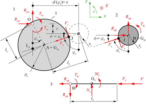
Table 3. Dynamic variables and parameters for the eccentric cam mechanism.

Parameter	Description
$T_{\mathrm{m}}$	Motor torque
$R_{x\mathrm{O}}$ and $R_{y\mathrm{O}},$ $R_{x\mathrm{B}}$ and $R_{y\mathrm{B}}$	Internal reaction forces in the revolute pairs O and B, respectively
$F_{\mathrm{n}}$	Internal normal force in the higher pair of contact point J
$F_{\mathrm{t}}$	Internal tangential force in the higher pair of contact point J, assuming no sliding
$N_3$ and $M_3$	Internal reaction normal force and moment in the prismatic pair, respectively
$T_{\mathrm{O}}$ and $T_{\mathrm{B}}$	Friction torques in the revolute pairs O and B, respectively
$c_{\mathrm{O}}$ and $c_{\mathrm{B}}$	Viscous friction coefficients in the revolute pairs O and B, respectively
$F_3$	Friction force in the prismatic pair
$c_3$	Viscous friction coefficient between the follower and the fixed guide
$F$	External force to avoid follower jump
$F_{\text{preload}}$	Preload force of the closure spring
$k_{\mathrm{s}}$	Linear stiffness of the closure spring
$m_{\text{1e}},$ $m_{\text{2r}}$ and $m_3$	Mass of the eccentric cam, the roller and the follower, respectively
$I_{\mathrm{O}}$	Eccentric cam moment of inertia along the z-axis referring to the rotational center O
$I_{{\mathrm{G}}_{2\mathrm{r}}}$	Roller moment of inertia along the z-axis referring to its center of inertia (${\mathrm{G}}_{2\mathrm{r}}$)

Equations (25–33) are obtained using vector theorems for each movable link of the mechanism. Sliding is assumed to be null at contact point J. (25) $$R_{x\mathrm{O}}-F_{\mathrm{n}}\hspace{0.17em}\mathrm{\text{cos}}\hspace{0.17em}{\phi }_2+F_{\mathrm{t}}\hspace{0.17em}\mathrm{\text{sin}}\hspace{0.17em}{\phi }_2=m_{1\mathrm{e}}\left({\ddot{\phi }}_1{l}_1\hspace{0.17em}\mathrm{\text{cos}}\hspace{0.17em}{\phi }_1-{\dot{\phi }}_1^2{l}_1\hspace{0.17em}\mathrm{\text{sin}}\hspace{0.17em}{\phi }_1\right)$$(25) (26) $$R_{y\mathrm{O}}-F_{\mathrm{n}}\hspace{0.17em}\mathrm{\text{sin}}\hspace{0.17em}{\phi }_2-F_{\mathrm{t}}\hspace{0.17em}\mathrm{\text{cos}}\hspace{0.17em}{\phi }_2=m_{1\mathrm{e}}\left({\ddot{\phi }}_1{l}_1\hspace{0.17em}\mathrm{\text{sin}}\hspace{0.17em}{\phi }_1+{\dot{\phi }}_1^2{l}_1\hspace{0.17em}\mathrm{\text{cos}}\hspace{0.17em}{\phi }_1\right)$$(26) (27) $$\begin{array}{l}{T}_{\mathrm{m}}-T_{\mathrm{O}}+F_{\mathrm{n}}\left(-\hspace{0.17em}\mathrm{\text{cos}}\hspace{0.17em}{\phi }_2\left(\epsilon +r_{\mathrm{r}}\hspace{0.17em}\mathrm{\text{sin}}\hspace{0.17em}{\phi }_2\right)-\hspace{0.17em}\mathrm{\text{sin}}\hspace{0.17em}{\phi }_2\left(d-r_{\mathrm{r}}\hspace{0.17em}\mathrm{\text{cos}}\hspace{0.17em}{\phi }_2\right)\right)\\ +F_{\mathrm{t}}\left(\hspace{0.17em}\mathrm{\text{sin}}\hspace{0.17em}{\phi }_2\left(\epsilon +r_{\mathrm{r}}\hspace{0.17em}\mathrm{\text{sin}}\hspace{0.17em}{\phi }_2\right)-\hspace{0.17em}\mathrm{\text{cos}}\hspace{0.17em}{\phi }_2\left(d-r_{\mathrm{r}}\hspace{0.17em}\mathrm{\text{cos}}\hspace{0.17em}{\phi }_2\right)\right)=I_{\mathrm{O}}{\ddot{\phi }}_1\end{array}$$(27) (28) $$R_{x\mathrm{B}}+F_{\mathrm{n}}\hspace{0.17em}\mathrm{\text{cos}}\hspace{0.17em}{\phi }_2-F_{\mathrm{t}}\hspace{0.17em}\mathrm{\text{sin}}\hspace{0.17em}{\phi }_2=m_{2\mathrm{r}}\ddot{d}$$(28) (29) $$R_{y\mathrm{B}}+F_{\mathrm{n}}\hspace{0.17em}\mathrm{\text{sin}}\hspace{0.17em}{\phi }_2+F_{\mathrm{t}}\hspace{0.17em}\mathrm{\text{cos}}\hspace{0.17em}{\phi }_2=0$$(29) (30) $$T_{\mathrm{B}}-F_{\mathrm{t}}{r}_{\mathrm{r}}=-I_{{\mathrm{G}}_{2\mathrm{r}}}{\ddot{\phi }}_{\mathrm{r}}$$(30) (31) $$-R_{x\mathrm{B}}-F_3-F=m_3\ddot{d}$$(31) (32) $$-R_{y\mathrm{B}}+N_3=0$$(32) (33) $$-T_{\mathrm{B}}+N_3\frac{l_3}{2}+M_3=0$$(33)

The friction torque $T_{\mathrm{O}}$ is calculated as in the former case using Eq. (14)(14) $$T_{\mathrm{O}}=c_{\mathrm{O}}{\dot{\phi }}_1$$(14) and the friction torque $T_{\mathrm{B}}$ is calculated using Eq. (34)(34) $$T_{\mathrm{B}}=c_{\mathrm{B}}{\dot{\phi }}_{\mathrm{r}}$$(34) , where ${\dot{\phi }}_{\mathrm{r}}$ is the angular velocity of the roller. (34) $$T_{\mathrm{B}}=c_{\mathrm{B}}{\dot{\phi }}_{\mathrm{r}}$$(34)

If the roller rotation is blocked, sliding at the cam-roller contact will occur. The modulus of the sliding velocity $v_{\text{slid}}$ is calculated as $v_{\text{slid}}=\left|\overline{{\mathbf{I}}_{\mathbf{13}}\mathbf{J}}\right|{\dot{\phi }}_1$ using Eq. (35)(35) $$v_{\text{slid}}=\left(\sqrt{d^2+{\left(d^{\prime }-\epsilon \right)}^2}-r_{\mathrm{r}}\right){\dot{\phi }}_1$$(35) , as can be deduced from Fig. 3. (35) $$v_{\text{slid}}=\left(\sqrt{d^2+{\left(d^{\prime }-\epsilon \right)}^2}-r_{\mathrm{r}}\right){\dot{\phi }}_1$$(35)

If the roller can rotate freely around revolute pair B, and assuming no sliding at the cam-roller contact, the roller rotates with an angular velocity ${\dot{\phi }}_{\mathrm{r}}=v_{\text{slid}}/r_{\mathrm{r}}.$ We calculate ${\dot{\phi }}_{\mathrm{r}}$ using Eq. (35)(35) $$v_{\text{slid}}=\left(\sqrt{d^2+{\left(d^{\prime }-\epsilon \right)}^2}-r_{\mathrm{r}}\right){\dot{\phi }}_1$$(35) , and the angular acceleration of the roller ${\ddot{\phi }}_r$ is obtained as the first temporal derivative of Eq. (36)(36) $${\dot{\phi }}_{\mathrm{r}}=\frac{\left(\sqrt{d^2+{\left(d^{\prime }-\epsilon \right)}^2}-r_{\mathrm{r}}\right)}{r_{\mathrm{r}}}{\dot{\phi }}_1$$(36) . (36) $${\dot{\phi }}_{\mathrm{r}}=\frac{\left(\sqrt{d^2+{\left(d^{\prime }-\epsilon \right)}^2}-r_{\mathrm{r}}\right)}{r_{\mathrm{r}}}{\dot{\phi }}_1$$(36) (37) $${\ddot{\phi }}_{\mathrm{r}}=\frac{d\cdot d^{\prime }+\left(d^{\prime }-\epsilon \right)d^{″}}{\sqrt{d^2+{\left(d^{\prime }-\epsilon \right)}^2}}\cdot \frac{{\dot{\phi }}_1{}^2}{r_{\mathrm{r}}}+\frac{\sqrt{d^2+{\left(d^{\prime }-\epsilon \right)}^2}-r_{\mathrm{r}}}{r_{\mathrm{r}}}{\ddot{\phi }}_1$$(37)

The friction force $F_3$ is calculated analogously to the former case using Eq. (17)(17) $$F_3=c_3\dot{x}$$(17) , being aware that $\dot{x}=\dot{d}.$

The external force $F$ is required to avoid follower jump in a force-closure cam mechanism. This force is provided with a linear spring using Eq. (38)(38) $$F=F_{\text{preload}}+k_{\mathrm{s}}\left(d-d_{\mathrm{\text{min}}}\right)$$(38) , where $d_{\mathrm{\text{min}}}$ is the minimum dead point from $d({\phi }_1),$ obtained using Eq. (39)(39) $$d_{\mathrm{\text{min}}}=\sqrt{r_{\mathrm{p}}{}^2-{\epsilon }^2}$$(39) . (38) $$F=F_{\text{preload}}+k_{\mathrm{s}}\left(d-d_{\mathrm{\text{min}}}\right)$$(38) (39) $$d_{\mathrm{\text{min}}}=\sqrt{r_{\mathrm{p}}{}^2-{\epsilon }^2}$$(39) If the external force is provided by a compression spring, it does not affect the energy loss per cycle because it is assumed to be a conservative force. Eq. (40)(40) $$E_{\text{loss}}=\oint \left({\mathit{T}}_{\mathit{O}}\cdot {\dot{\mathit{\phi }}}_1+{\mathit{T}}_{\mathit{B}}\cdot {\dot{\mathit{\phi }}}_{\mathit{r}}+{\mathit{F}}_3\cdot \dot{\mathit{d}}\right)\mathrm{d}t$$(40) evaluates the total energy loss $E_{\text{loss}}$ per cycle. (40) $$E_{\text{loss}}=\oint \left({\mathit{T}}_{\mathit{O}}\cdot {\dot{\mathit{\phi }}}_1+{\mathit{T}}_{\mathit{B}}\cdot {\dot{\mathit{\phi }}}_{\mathit{r}}+{\mathit{F}}_3\cdot \dot{\mathit{d}}\right)\mathrm{d}t$$(40)

Equation (40)(40) $$E_{\text{loss}}=\oint \left({\mathit{T}}_{\mathit{O}}\cdot {\dot{\mathit{\phi }}}_1+{\mathit{T}}_{\mathit{B}}\cdot {\dot{\mathit{\phi }}}_{\mathit{r}}+{\mathit{F}}_3\cdot \dot{\mathit{d}}\right)\mathrm{d}t$$(40) considers no energy loss associated with sliding velocities at the cam-roller contact, as assumed in others studies (Sanmiguel-Rojas and Hidalgo-Martínez 2016). Nevertheless, to validate this assumption, a model to evaluate energy loss due to sliding and elastic deformation is presented. The friction force in the direction of the sliding velocity $F_{\text{slid}}$ is obtained using Eq. (41)(41) $$F_{\text{slid}}=\mu F_{\mathrm{n}}$$(41) , where $\mu$ is a traction coefficient calculated according to Masjedi and Khonsari (2015). Their friction model considers elastic deformations at the contact, which requires to determine internal reactions in pairs, for example using vector theorems. The substitution of the internal tangential force $F_{\mathrm{t}}$ for $F_{\text{slid}}$ is required in Eqs. (25–30). (41) $$F_{\text{slid}}=\mu F_{\mathrm{n}}$$(41)

The energy loss $E_{\text{loss\hspace{0.17em}slid}}$ per cycle for the higher pair is calculated with Eq. (42)(42) $$E_{\text{loss slid}}=\oint {\mathit{F}}_{\text{slid}}·\text{SRR}·{\mathit{v}}_{\text{slid}}\mathrm{d}t$$(42) , as the integral of instantaneous power loss, $E_{\text{loss\hspace{0.17em}slid}}=\oint P_{\text{loss\hspace{0.17em}slid}}\mathrm{d}t,$ where SRR is a slide-to-roll ratio (SRR) (Alakhramsing et al. 2018a, 2018b; Gromadova 2021) and $v_{\text{slid}}$ is the sliding velocity calculated with Eq. (35)(35) $$v_{\text{slid}}=\left(\sqrt{d^2+{\left(d^{\prime }-\epsilon \right)}^2}-r_{\mathrm{r}}\right){\dot{\phi }}_1$$(35) . (42) $$E_{\text{loss slid}}=\oint {\mathit{F}}_{\text{slid}}·\text{SRR}·{\mathit{v}}_{\text{slid}}\mathrm{d}t$$(42)

3. Simulation results

In this Section, we first compare a slider-crank mechanism with specific dimensions to two alternatives of eccentric cam mechanisms in terms of the total energy loss per cycle, the internal reactions in pairs and the transmission efficiency of force. Secondly, we solve a range of geometrical parameter scales required for these mechanisms and plot workspaces used to: i) determine which presents the lowest values of $E_{\text{loss}},$ a slider-crank or an eccentric cam mechanism; and ii) identify trends in how modifying geometrical parameters affects $E_{\text{loss}}.$

3.1. Case study

Table 4 summarizes the required parameters for the chosen slider-crank mechanism and the two equivalent eccentric cam mechanisms: one with a smaller roller radius than the eccentric cam radius of curvature; and one with a larger roller radius than the eccentric cam radius of curvature. These three mechanisms, with parameters shown in Table 4, are assembled on the experimental test stand, as explained in Section 4.

Table 4. Required parameters for the numerical examples.

Slider-crank mechanism		Eccentric cam. Small roller radius		Eccentric cam. Big roller radius
Parameter	Value	Parameter	Value	Parameter	Value
$l_1$ [mm]	25
$l_2$ [mm]	85	$r_{\mathrm{r}}$ [mm]	18.5	$r_{\mathrm{r}}$ [mm]	51
		${\rho }_{\mathrm{c}}$ [mm]	66.5	${\rho }_{\mathrm{c}}$ [mm]	34
$l_3$ [mm]	184.5
$\epsilon$ [mm]	0
${\dot{\phi }}_1$ [rad/s]	36.65
${\ddot{\phi }}_1$ [rad/s^2]	0
$m_1$ [kg]	0.031	$m_{1\mathrm{e}}$ [kg]	1.71	$m_{1\mathrm{e}}$ [kg]	0.41
$I_{{\mathrm{G}}_1}$ [kg·m^2]	9.5·10^−6	$I_{\mathrm{O}}$ [kg·m^2]	4.9·10^-3	$I_{\mathrm{O}}$ [kg·m^2]	4.9·10^-4
$m_2$ [kg]	0.094	$m_{2\mathrm{r}}$ [kg]	0.093	$m_{2\mathrm{r}}$ [kg]	0.53
$I_{{\mathrm{G}}_2}$ [kg·m^2]	9.2·10^−5	$I_{{\mathrm{G}}_{2\mathrm{r}}}$ [kg·m^2]	1.9·10^-5	$I_{{\mathrm{G}}_{2\mathrm{r}}}$ [kg·m^2]	8·10^-4
$m_3$ [kg]	1.3
$c_{\mathrm{O}}$ [N·m/(rad/s)]	0.17
$c_{\mathrm{A}}$ [N·m/(rad/s)]	0.026	No		No
$c_{\mathrm{B}}$ [N·m/(rad/s)]	0.026
$c_3$ [N/(m/s)]	24.40
$F_{\text{pre}}$ [N]	66.42
$k_{\mathrm{s}}$ [kN/m]	1.23

To facilitate $E_{\text{loss}}$ comparison between these kinematically equivalent mechanisms, we consider:

• All mechanisms have the same lubrication conditions. Revolute pair O is grease-sealed lubricated. Revolute pairs A, B, the prismatic pair and the higher pair are lubricated with Vaseline oil (Krafft n.d.).

• In all mechanisms there exist the revolute pairs O, B and the prismatic pair, so the same viscous friction coefficients $c_{\mathrm{O}},$ $c_{\mathrm{B}}$ and $c_3$ are assumed, as can be observed in Table 4. Their experimental determination is explained in Appendix A.

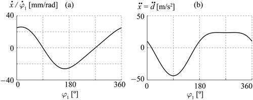
Figure 5(a) shows the transmission efficiency of motion evaluated as the ratio between the output linear velocity $\dot{x}$ and the input angular velocity ${\dot{\phi }}_1.$ Figure 5(b) shows the linear acceleration of the follower and the slider, $\ddot{x}=\ddot{d},$ required for vector theorems. For the three mechanisms both curves are the same because they are kinematically equivalent mechanisms.

Figure 5. (a) Transmission efficiency of motion; (b) Linear acceleration of the slider and the follower.

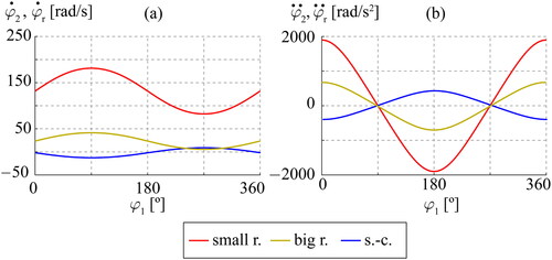
Figure 6(a) and (b) shows the angular velocities ${\dot{\phi }}_{\mathrm{r}}$ and the angular accelerations ${\ddot{\phi }}_{\mathrm{r}}$ for both eccentric cam mechanisms, respectively. The rod’s angular velocities ${\dot{\phi }}_2$ and angular accelerations ${\ddot{\phi }}_2$ of the slider-crank mechanism are also depicted.

Figure 6. Rollers and rod: (a) Angular velocities; (b) Angular accelerations.

Figure 7(a)-(c) depicts the internal reactions in each pair, that require solving vector theorems. Figure 7(d) depicts the transmission efficiency of force evaluated as the ratio between the external force $F$ (output force) and the input torque motor $T_{\mathrm{m}}.$

Figure 7. Internal reactions for each pair: (a) Slider-crank; (b) Eccentric cam with small roller radius; (c) Eccentric cam with big roller radius; (d) Transmission efficiency of force.

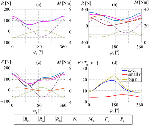
For all the pairs, the case with the highest internal reactions is the eccentric cam mechanism with the small roller radius. The slider-crank mechanism and the eccentric cam mechanism with the big roller radius present similar curve shapes for the internal reactions in the common pairs, despite values being slightly lower for the slider-crank mechanism. The mechanism with the best transmission efficiency of force (highest values) is the eccentric cam mechanism with the big roller radius, followed closely by the slider-crank mechanism.

If deformation and sliding are considered, the friction force in the direction of the sliding velocity $F_{\text{slid}}$ is obtained using Eq. (41)(41) $$F_{\text{slid}}=\mu F_{\mathrm{n}}$$(41) , with the mean value of the normal force $F_{\mathrm{n}},$ being 94 N and 93 N according to Fig. 7(b)-(c) for the eccentric cam with the big roller radius and the small roller radius, respectively. An SRR = 5% is assumed, which is a maximum case compared to other studies of cam mechanisms (Alakhramsing et al. 2018b; Norton 2002). Table 5 presents the values required to calculate $\mu ,$ some obtained from the eccentric cam mechanism assembled on the experimental test stand explained in Section 4. The traction coefficients are 0.046 and 0.014 for the big and small roller radii cases, respectively.

Table 5. Required parameters for traction coefficient (Masjedi and Khonsari 2015).

Parameter	Value/specification
Contact length	0.013 m
$R,$ Equivalent contact radius	Calculated with eccentric cam radius and roller radius from Table 4
$E^{\prime },$ Effective Young’s modulus	228 GPa
Thermal conductivity of contact solids	60.5 W/(m·K)
Specific heat of contact solids	434 J/(kg·K)
Vickers hardness	2.35 GPa
$R_{\mathrm{a}},$ Surface roughness	0.2 µm
Limiting shear stress coefficient	0.0434
Asperity friction coefficient	0.12
SRR	0.05
$v_{\text{slid}},$ Mean sliding velocity big roller	1.25 m/s·SRR = 0.063 m/s
$v_{\text{slid}},$ Mean sliding velocity small roller	2.4 m/s·SRR = 0.12 m/s
Oil density	0.87 g/ml
Oil kinematic viscosity	20.5 mm^2/s at 40 °C
Inlet lubricant temperature	315 K
Viscosity temperature coefficient	0.027 K^-1
Viscosity pressure coefficient	1.5·10^-8 m^2/N

Using Eq. (42)(42) $$E_{\text{loss slid}}=\oint {\mathit{F}}_{\text{slid}}·\text{SRR}·{\mathit{v}}_{\text{slid}}\mathrm{d}t$$(42) , $E_{\text{loss\hspace{0.17em}slid}}$ values are 0.04 and 0.03 J for the eccentric cam with the big and small roller radii, respectively. These negligible levels in $E_{\text{loss\hspace{0.17em}slid}}$ associated with the sliding friction force component and elastic deformation agree with Alakhramsing et al. (2018a, 2018b, 2019).

Figure 8 depicts the $E_{\text{loss}}$ per cycle. For the slider-crank mechanism, we use Eq. (18)(18) $$E_{\text{loss}}=\oint \left({\mathit{T}}_{\mathit{O}}\cdot {\dot{\mathit{\phi }}}_1+{\mathit{T}}_{\mathit{A}}\cdot {\dot{\mathit{\phi }}}_1+{\mathit{T}}_{\mathit{A}}\cdot {\dot{\mathit{\phi }}}_2+{\mathit{T}}_{\mathit{B}}\cdot {\dot{\mathit{\phi }}}_2+{\mathit{F}}_3\cdot \dot{\mathit{x}}\right)\mathrm{d}t$$(18) and for the eccentric cams, Eq. (40)(40) $$E_{\text{loss}}=\oint \left({\mathit{T}}_{\mathit{O}}\cdot {\dot{\mathit{\phi }}}_1+{\mathit{T}}_{\mathit{B}}\cdot {\dot{\mathit{\phi }}}_{\mathit{r}}+{\mathit{F}}_3\cdot \dot{\mathit{d}}\right)\mathrm{d}t$$(40) .

Figure 8. Energy loss per cycle.

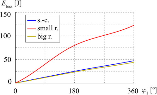
The mechanism with the lowest $E_{\text{loss}}$ is the eccentric cam with the big roller radius (44.3 J), then the slider-crank (47.4 J, a 7% increase), and finally the eccentric cam with the small roller radius (122.5 J, a 175% increase).

The amount of $E_{\text{loss}}$ added by revolute pair O and the prismatic pair are the same for all three mechanisms. The differences come from revolute pairs A and B. Revolute pair A contributes to $E_{\text{loss}}$ only in the slider-crank. For both eccentric cams, we assume that the higher pair contribution is null. The differences in relative angular velocities (Fig. 6(a)) affect the values of $E_{\text{loss}}$ associated with revolute pair B. Even though the eccentric cam with the big roller radius has a higher $E_{\text{loss}}$ at revolute pair B, its contribution is lower than the one from revolute pair A of the slider-crank.

3.2. Energy loss comparison workspaces

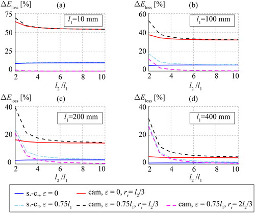
In this Section we present the energetic comparison between the analyzed mechanisms by means of plotting two workspaces. These allow for a sensitivity analysis of $E_{\text{loss}}$ against a range of the main geometrical parameters.

For a slider-crank, the output motion of slider $x$ is a function of $l_1,$ $l_2,$ and $\epsilon .$ For an eccentric cam, we obtain the prime circle as $r_{\mathrm{p}}=l_2-l_1;$ thus, only the radius of the roller $r_{\mathrm{r}}$ is needed as an extra parameter.

Restrictions (43)(43) $$10\text{mm}\le l_1\le 400\text{mm}$$(43) to (46)(46) $$l_2/3\le r_{\mathrm{r}}\le 2l_2/3$$(46) define the imposed conditions between the four geometric parameters. (43) $$10\text{mm}\le l_1\le 400\text{mm}$$(43) (44) $$2l_1\le l_2\le 10l_1$$(44) (45) $$l_2\ge 2l_1+\epsilon$$(45) (46) $$l_2/3\le r_{\mathrm{r}}\le 2l_2/3$$(46)

The crank length $l_1$ is the input parameter. For the offset of the slider $\epsilon$ only two extreme cases are studied: $\epsilon =0$ and $\epsilon =0.75l_1.$ Restriction (45)(45) $$l_2\ge 2l_1+\epsilon$$(45) ensures a full crank rotation and pressure angle recommendations, ${\phi }_2\le 30º.$ Restriction (46)(46) $$l_2/3\le r_{\mathrm{r}}\le 2l_2/3$$(46) ensures the cam pitch curve (${\rho }_{\mathrm{p}}=l_2$) recommendations by imposing values for roller radius $r_{\mathrm{r}}.$

Figure 9 shows $E_{\text{loss}}$ for the three mechanisms. The values imposed on ${\dot{\phi }}_1$ and the viscous friction coefficients are the ones shown in Table 4.

Figure 9. Energy loss per cycle workspaces.

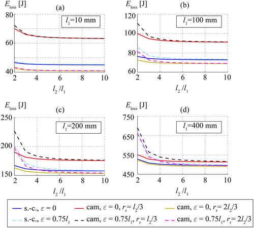
In Fig. 9, the comparison must be done individually for each crank length $l_1.$ The conclusions to reduce energy loss per cycle are:

• The most favorable cases are always for the eccentric cam with the largest roller radius ($r_{\mathrm{r}}=2l_2/3$) and null offset ($\epsilon =0$). $E_{\text{loss}}$ is slightly higher for the slider-crank with the null offset. The reduction of the roller radius ($r_{\mathrm{r}}=l_2/3$) causes an increment of the angular velocity of the roller ${\dot{\phi }}_{\mathrm{r}}$ (Fig. 6(a)). Therefore, the $E_{\text{loss}}$ associated with revolute pair B increases.

• The non-null offset cases have higher $E_{\text{loss}}$ than the null ones.

Figure 10 depicts the relative differences with regard to the most efficient case. We conclude that the maximum differences in $E_{\text{loss}}$ are obtained for small-sized mechanisms ($l_1$ around 10 mm) and for low $l_2/l_1$ ratios (Fig. 10(a)).

Figure 10. Relative differences in energy loss per cycle with regard to the most efficient case.

4. Experimental results

4.1. Test stand description

The test stand shown in Fig. 11 was built to validate the classification in terms of $E_{\text{loss}}$ observed with the simulated results: the best alternative is the eccentric cam mechanism with the big roller radius, then the slider-crank mechanism, and finally the eccentric cam mechanism with the small roller radius. The mechanisms can be assembled by sharing the following common elements: 1) fixed frame; 2) DC motor with a double stage gear reduction; 3) shaft coupling; 4) flywheel; 5) main shaft; 6) final shaft coupling; and 7) translational output element with a closure spring. The mechanism under study is assembled through the final shaft coupling, where the crank is embedded. The test stand includes two inductive sensors. The first one (highlighted in green in Fig. 11) points outward to a 30-tooth pulley fixed to the main shaft, which acts as an angular digital encoder. The angular velocity of the main shaft ${\dot{\phi }}_1$ is obtained as the first temporal derivative of this measure. The second inductive sensor (highlighted in red in Fig. 11) points outward to the translational output element. It is used to output a step signal per cycle. Measurements are recorded by a digital signal analyzer with a 2 MHz sampling rate. Table 6 gathers information about the shared components for this test stand.

Figure 11. Test stand indicating the shared common elements.

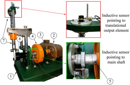
Table 6. Test stand specifications of the shared components.

Element	Specification
DC Motor	DC shunt motor. P = 232 W; I = 1.8 A; U = 220 V
Gear reducer	2 stage reduction: worm gear and spur gears i = (31·38)/(5·51) = 4.619
Main shaft	$I_{{\mathrm{G}}_{\text{ms}}}=$5.4·10^-4kg·m^2
Flywheel	$I_{{\mathrm{G}}_{\mathrm{f}}}=$7.2·10^-2kg·m^2
Final shaft coupling	$I_{{\mathrm{G}}_{\text{fsc}}}=$1.8·10^-3kg·m^2

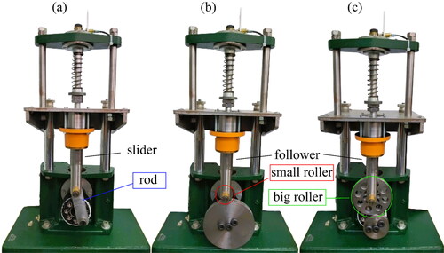
Figure 12 shows the three kinematically equivalent mechanisms assembled on the test stand. Mechanism parameters and lubrication conditions are those explained in Section 3.1.

Figure 12. (a) Slider-crank; (b) Eccentric cam with small roller radius; (c) Eccentric cam with big roller radius.

4.2. Comparison of energy loss per cycle

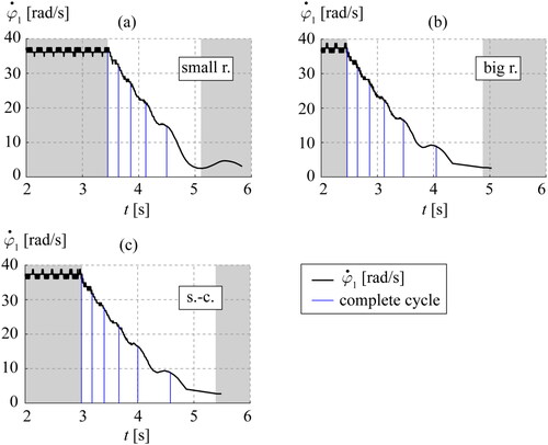
All experimental tests begin in a stationary regime, then the machine is switched off and the transient period is recorded until standstill. Figure 13 shows an example for each mechanism. The left grey region indicates the initial stationary regime. The right grey region indicates a rebound of the translational output elements due to the follower closure spring just before standstill. The blue lines indicate a complete cycle.

Figure 13. Test results: (a) Eccentric cam with small roller radius; (b) Eccentric cam with big roller radius; (c) Slider-crank.

The experimental comparison of energy loss per cycle is carried out by applying the work-energy theorem using Eq. (47)(47) $${\Delta E_{\mathrm{k}}]}_1^2={\sum W_{\text{loss}}]}_1^2$$(47) . The theorem is applied over the whole system between two different mechanical states, 1 and 2, which correspond to an entire number of complete cycles of ${\phi }_1.$ Notice that, for an entire cycle, the work carried out by conservative forces is null. (47) $${\Delta E_{\mathrm{k}}]}_1^2={\sum W_{\text{loss}}]}_1^2$$(47)

We obtain the variation in the kinetic energy ${\Delta E_{\mathrm{k}}]}_1^2$ via Eq. (48)(48) $${\Delta E_{\mathrm{k}}]}_1^2=\frac{1}{2}{I}_{\text{red}{\phi }_1}\left({{\dot{\phi }}_1^2|}_2-{{\dot{\phi }}_1^2|}_1\right)$$(48) , where: $I_{\text{red\hspace{0.17em}}{\phi }_1}$ is the inertia of the whole system reduced to the angular coordinate ${\phi }_1,$ ${{\dot{\phi }}_1|}_2$ is the angular velocity at the end of a cycle (state 2), and ${{\dot{\phi }}_1|}_1$ is the angular velocity at the beginning of a cycle (state 1). (48) $${\Delta E_{\mathrm{k}}]}_1^2=\frac{1}{2}{I}_{\text{red}{\phi }_1}\left({{\dot{\phi }}_1^2|}_2-{{\dot{\phi }}_1^2|}_1\right)$$(48)

For the slider-crank $I_{\text{red\hspace{0.17em}}{\phi }_1}$ is calculated using Eq. (49)(49) $$\begin{array}{c}{I}_{\text{red\hspace{0.17em}}{\phi }_1}=I_{{\mathrm{G}}_{\text{ms}}}+I_{{\mathrm{G}}_{\mathrm{f}}}+I_{{\mathrm{G}}_{\text{fsc}}}+m_2{l}_1^2\left(1-\frac{\hspace{0.17em}\mathrm{\text{sin}}\hspace{0.17em}{\phi }_1}{\hspace{0.17em}\mathrm{\text{cos}}\hspace{0.17em}{\phi }_2}\mathrm{\text{sin}}\hspace{0.17em}\left({\phi }_1-{\phi }_2\right)+\frac{1}{4}\frac{{\hspace{0.17em}\mathrm{\text{sin}}\hspace{0.17em}}^2{\phi }_1}{{\hspace{0.17em}\mathrm{\text{cos}}\hspace{0.17em}}^2{\phi }_2}\right)+\\ l_1^2\left(\frac{I_{{\mathrm{G}}_2}}{l_2^2}·\frac{{\hspace{0.17em}\mathrm{\text{sin}}\hspace{0.17em}}^2{\phi }_1}{{\hspace{0.17em}\mathrm{\text{cos}}\hspace{0.17em}}^2{\phi }_2}+m_3\frac{{\hspace{0.17em}\mathrm{\text{cos}}\hspace{0.17em}}^2\left({\phi }_1-{\phi }_2\right)}{{\hspace{0.17em}\mathrm{\text{cos}}\hspace{0.17em}}^2{\phi }_2}\right)\end{array}$$(49) and for the eccentric cam mechanisms $I_{\text{red\hspace{0.17em}}{\phi }_1}$ is calculated with Eq. (50)(50) $$\begin{array}{c}{I}_{\text{red\hspace{0.17em}}{\phi }_1}=I_{{\mathrm{G}}_{\text{ms}}}+I_{{\mathrm{G}}_{\mathrm{f}}}+I_{{\mathrm{G}}_{\text{fsc}}}+\\ I_{{\mathrm{G}}_{1\mathrm{e}}}+I_{{\mathrm{G}}_{2\mathrm{r}}}{C}^2+l_1^2\left(m_{1\mathrm{e}}+m_{2\mathrm{r}}\frac{{\hspace{0.17em}\mathrm{\text{cos}}\hspace{0.17em}}^2\left({\phi }_1-{\phi }_2\right)}{{\hspace{0.17em}\mathrm{\text{cos}}\hspace{0.17em}}^2{\phi }_2}+m_3\frac{{\hspace{0.17em}\mathrm{\text{cos}}\hspace{0.17em}}^2\left({\phi }_1-{\phi }_2\right)}{{\hspace{0.17em}\mathrm{\text{cos}}\hspace{0.17em}}^2{\phi }_2}\right)\end{array}$$(50) , where C is obtained using Eq. (51)(51) $$C=\frac{\left(\sqrt{{\left(l_1\hspace{0.17em}\mathrm{\text{sin}}\hspace{0.17em}{\phi }_1+l_2\hspace{0.17em}\mathrm{\text{cos}}\hspace{0.17em}\left(\mathrm{\text{arcsin}}\left(\frac{l_1\hspace{0.17em}\mathrm{\text{cos}}\hspace{0.17em}{\phi }_1-\epsilon }{l_2}\right)\right)\right)}^2+{\left(l_1\left(\hspace{0.17em}\mathrm{\text{cos}}\hspace{0.17em}{\phi }_1+\frac{\left(l_1\hspace{0.17em}\mathrm{\text{cos}}\hspace{0.17em}{\phi }_1-\epsilon \right)\hspace{0.17em}\mathrm{\text{sin}}\hspace{0.17em}{\phi }_1}{l_2\sqrt{1-{\left(\frac{l_1\hspace{0.17em}\mathrm{\text{cos}}\hspace{0.17em}{\phi }_1-\epsilon }{l_2}\right)}^2}}\right)-\epsilon \right)}^2}-r_{\mathrm{r}}\right)}{r_{\mathrm{r}}}$$(51) . ${\phi }_2$ is dependent on ${\phi }_1$ according to Eq. (2)(2) $$-l_1\hspace{0.17em}\mathrm{\text{cos}}\hspace{0.17em}{\phi }_1+l_2\hspace{0.17em}\mathrm{\text{sin}}\hspace{0.17em}{\phi }_2+\epsilon =0$$(2) . The moment of inertia of the eccentric cam, along the z-axis, referring to its center of inertia ($I_{{\mathrm{G}}_{1\mathrm{e}}}$) is 3.9·10⁻³ kg·m² and 2.5·10⁻⁴ kg·m² for the small and big roller mechanisms, respectively. (49) $$\begin{array}{c}{I}_{\text{red\hspace{0.17em}}{\phi }_1}=I_{{\mathrm{G}}_{\text{ms}}}+I_{{\mathrm{G}}_{\mathrm{f}}}+I_{{\mathrm{G}}_{\text{fsc}}}+m_2{l}_1^2\left(1-\frac{\hspace{0.17em}\mathrm{\text{sin}}\hspace{0.17em}{\phi }_1}{\hspace{0.17em}\mathrm{\text{cos}}\hspace{0.17em}{\phi }_2}\mathrm{\text{sin}}\hspace{0.17em}\left({\phi }_1-{\phi }_2\right)+\frac{1}{4}\frac{{\hspace{0.17em}\mathrm{\text{sin}}\hspace{0.17em}}^2{\phi }_1}{{\hspace{0.17em}\mathrm{\text{cos}}\hspace{0.17em}}^2{\phi }_2}\right)+\\ l_1^2\left(\frac{I_{{\mathrm{G}}_2}}{l_2^2}·\frac{{\hspace{0.17em}\mathrm{\text{sin}}\hspace{0.17em}}^2{\phi }_1}{{\hspace{0.17em}\mathrm{\text{cos}}\hspace{0.17em}}^2{\phi }_2}+m_3\frac{{\hspace{0.17em}\mathrm{\text{cos}}\hspace{0.17em}}^2\left({\phi }_1-{\phi }_2\right)}{{\hspace{0.17em}\mathrm{\text{cos}}\hspace{0.17em}}^2{\phi }_2}\right)\end{array}$$(49) (50) $$\begin{array}{c}{I}_{\text{red\hspace{0.17em}}{\phi }_1}=I_{{\mathrm{G}}_{\text{ms}}}+I_{{\mathrm{G}}_{\mathrm{f}}}+I_{{\mathrm{G}}_{\text{fsc}}}+\\ I_{{\mathrm{G}}_{1\mathrm{e}}}+I_{{\mathrm{G}}_{2\mathrm{r}}}{C}^2+l_1^2\left(m_{1\mathrm{e}}+m_{2\mathrm{r}}\frac{{\hspace{0.17em}\mathrm{\text{cos}}\hspace{0.17em}}^2\left({\phi }_1-{\phi }_2\right)}{{\hspace{0.17em}\mathrm{\text{cos}}\hspace{0.17em}}^2{\phi }_2}+m_3\frac{{\hspace{0.17em}\mathrm{\text{cos}}\hspace{0.17em}}^2\left({\phi }_1-{\phi }_2\right)}{{\hspace{0.17em}\mathrm{\text{cos}}\hspace{0.17em}}^2{\phi }_2}\right)\end{array}$$(50) (51) $$C=\frac{\left(\sqrt{{\left(l_1\hspace{0.17em}\mathrm{\text{sin}}\hspace{0.17em}{\phi }_1+l_2\hspace{0.17em}\mathrm{\text{cos}}\hspace{0.17em}\left(\mathrm{\text{arcsin}}\left(\frac{l_1\hspace{0.17em}\mathrm{\text{cos}}\hspace{0.17em}{\phi }_1-\epsilon }{l_2}\right)\right)\right)}^2+{\left(l_1\left(\hspace{0.17em}\mathrm{\text{cos}}\hspace{0.17em}{\phi }_1+\frac{\left(l_1\hspace{0.17em}\mathrm{\text{cos}}\hspace{0.17em}{\phi }_1-\epsilon \right)\hspace{0.17em}\mathrm{\text{sin}}\hspace{0.17em}{\phi }_1}{l_2\sqrt{1-{\left(\frac{l_1\hspace{0.17em}\mathrm{\text{cos}}\hspace{0.17em}{\phi }_1-\epsilon }{l_2}\right)}^2}}\right)-\epsilon \right)}^2}-r_{\mathrm{r}}\right)}{r_{\mathrm{r}}}$$(51)

Figure 14 plots $I_{\text{red\hspace{0.17em}}{\phi }_1}$ for the three mechanisms using the values from Table 4 and Table 6.

Figure 14. Inertia reduced to ${\phi }_1.$

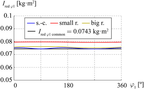
Even though $I_{\text{red\hspace{0.17em}}{\phi }_1}$ is function of ${\phi }_1,$ as a first approach, we assume that the inertia of the whole system is equivalent and constant between the three mechanisms. The contribution of the inertia of the shared elements $I_{\text{red\hspace{0.17em}}{\phi }_1\text{\hspace{0.17em}common}}=I_{{\mathrm{G}}_{\text{ms}}}+I_{{\mathrm{G}}_{\mathrm{f}}}+I_{{\mathrm{G}}_{\text{fsc}}}$ is constant and is much higher than the contribution of the inertia of the elements of each mechanism. The differences between the value of $I_{\text{red\hspace{0.17em}}{\phi }_1\text{\hspace{0.17em}common}}$ and the higher values are: for the slider-crank mechanism, 1.4%, for the eccentric cam with the big roller radius, 2.1% and for the eccentric cam with the small roller radius, 7.4%.

Assuming the same constant value of $I_{\text{red\hspace{0.17em}}{\phi }_1}$ for the three mechanisms, we can state that the energy loss per cycle ${\sum W_{\text{loss}}]}_1^2$ is, as a first approach, proportional to ${{\dot{\phi }}_1^2|}_2-{{\dot{\phi }}_1^2|}_1.$

Figure 15 shows ${{\dot{\phi }}_1^2|}_2-{{\dot{\phi }}_1^2|}_1$ as function of ${\dot{\phi }}_1,$ because when using a viscous friction model, energy losses vary as a function of relative velocities. The three sets of experiments for each mechanism carried out have been represented in Figure 15. On the right-hand side, a zoomed region around ${\dot{\phi }}_1=$30 rad/s is shown and the mean value of the three experiments per alternative is represented with a dot.

Figure 15. Experimental comparison of energy loss per cycle.

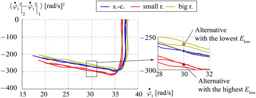
In Fig. 15, the starting point is at ${{\dot{\phi }}_1^2|}_2-{{\dot{\phi }}_1^2|}_1=0$ rad²/s², indicating that the system is in a stationary regime. It should be pointed out that the mean stationary angular velocity ${\dot{\phi }}_1$ using a small roller (around 36 rad/s) is lower than the angular velocity using a big roller or a slider-crank (around 37.5 rad/s). Moreover, the system speed in a stationary regime is sensitive to friction variations because the voltage of the DC motor is constant (controlled).

During the transient period, the variation of ${{\dot{\phi }}_1^2|}_2-{{\dot{\phi }}_1^2|}_1$ is a function of angular velocity, which agrees with a viscous friction model. The results shown in Fig. 15 ranks the alternatives in terms of reducing $E_{\text{loss}}$ per cycle. The best is the eccentric cam mechanism with the big roller radius, then the slider-crank mechanism, and finally the eccentric cam mechanism with the small roller radius. Furthermore, the derived experimental data show only slight differences between the slider-crank and the eccentric cam with the big roller radius. Both experimental trends agree with the trends presented for the simulated results in Section 3.1 and 3.2.

5. Conclusions

This study compares the total energy loss per cycle between kinematically equivalent slider-crank and eccentric cam mechanisms. Our aim is to provide machinery designers with the knowledge to evaluate energy losses in order to decide among the types of mechanisms and the values for geometrical parameters within a given system.

From our analysis we conclude that an eccentric cam mechanism, with a roller radius closer to 1.5 times the minimum cam pitch curve and without a follower offset, is the best solution to reduce the energy loss, while considering recommendations provided by Norton (2002) in order to avoid high Hertzian pressures. Furthermore, it also provides the best transmission efficiency of force. Reducing the roller radius and providing follower offset increase the total energy loss. For small mechanisms, the energy loss sensitivity is higher while modifying the geometrical parameters (crank length, rod-crank length ratio, roller radius and follower offset).

Based on our experimental validations we can conclude that a viscous friction model is an effective preliminary approach. If a deeper analysis is required to fine tune the amount of energy loss, more complex friction models could be used, despite then having to calculate internal reactions in pairs using for example vector theorems and while including other tribological parameters.

Finally, we consider that: i) the proposed methodology can be expanded to other cam mechanisms such as circular arc cams; and ii) the experimental approach presented to evaluate energy losses can be further used to compare with other planar one degree-of-freedom mechanisms or friction models.

Disclosure statement

No potential conflict of interest was reported by the author(s).

Appendix A.

Experimental determination of viscous friction coefficients

A.1 Determination of $c_3$

In the test carried out, the linear bushing in the prismatic pair has relative vertical motion while the translation output element of Fig. 11 is fixed. The bushing is between two springs in parallel as shown in Fig. A1(b).

Figure A1. Bushing oscillating system: (a) Base input test; (b) Schematic representation.

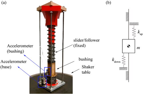
Figure A1(a) shows the test stand assembled to a shaker table to carry out a vibration test and experimentally obtain the damping coefficient of the bushing. To register input and output signals, two accelerometers are used: the input signal comes from the accelerometer located at the base; the output signal comes from the one attached to the bushing. As an input signal, a random acceleration (between 5 Hz and 300 Hz) with a power spectral density of 0.5 (m/s²)²/Hz is used. The sample frequency is 100 Hz recording for a 10 min period and the signals are processed within a 10 000 sample sliding window. The experimental viscous friction coefficient $c_3$ is 24.40 N/(m/s).

A.2 Determination of $c_{\mathrm{A}}$ and $c_{\mathrm{B}}$

The methodology applied is based on the steps described in Veciana, Jordi, and Lores (2021). A pendulum system shown in Fig. A2(a) is built for the experimental determination of the viscous damping friction coefficient of the flanged sintered bronze bushings used in revolute pairs A and B (Fig. 1). The revolute pair O is constructed using the same flanged sintered bronze bushing and the same steel cylindrical pin used in revolute pair B.

Figure A2. (a) Pendulum system; (b) Schematic representation.

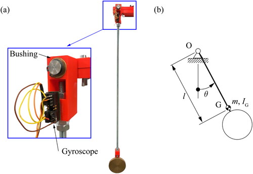
The linearized motion equation assuming small oscillations around $\theta =$0 is (A52) $$\left(m{l}^2+I_{\mathrm{G}}\right)\ddot{\theta }+c\dot{\theta }+\mathit{\text{mgl}}\theta =0$$(A52)

The values of the parameters used in Eq. (A52)(A52) $$\left(m{l}^2+I_{\mathrm{G}}\right)\ddot{\theta }+c\dot{\theta }+\mathit{\text{mgl}}\theta =0$$(A52) are: $m=$0.603 kg, $l=$492 mm and $I_{\mathrm{G}}=$2.62·10⁻²kg·m².

A set of 5 experiments is carried out, applying vaseline oil to the bushing (Krafft n.d.). The angular velocity ${\dot{\theta }}_{\hspace{0.17em}\mathrm{\text{exp}}\hspace{0.17em}}(t)$ is experimentally measured with a gyroscope attached to the pendulum bar. The analytical general solution ${\theta }_{\text{theo}}(t)$ of Eq. (A52)(A52) $$\left(m{l}^2+I_{\mathrm{G}}\right)\ddot{\theta }+c\dot{\theta }+\mathit{\text{mgl}}\theta =0$$(A52) is known and the first temporal derivative ${\dot{\theta }}_{\text{theo}}(t)$ is obtained. The parameters of ${\dot{\theta }}_{\text{theo}}(t)$ are obtained by minimizing the accumulated differences between ${\dot{\theta }}_{\text{theo}}(t)$ and ${\dot{\theta }}_{\hspace{0.17em}\mathrm{\text{exp}}\hspace{0.17em}}(t)$ using the least squares method as an objective function. Then, the viscous damping friction coefficient is determined as an optimized parameter of ${\dot{\theta }}_{\hspace{0.17em}\mathrm{\text{exp}}\hspace{0.17em}}(t).$ This is done for each set of experiments and the obtained mean value of $c_{\mathrm{A}}$ and $c_{\mathrm{B}}$ is 0.026 N·m/(rad/s).

A.3 Determination of $c_{\mathrm{O}}$

The test stand is mounted only with elements 1 to 6 of Fig. 11, without any of the compared mechanisms. The friction torque is obtained by rotating at low speed through indirect measure of the force (gauge) at the flywheel radius. The averaged experimental value of $c_{\mathrm{O}}$ is 0.17 N·m/(rad/s). This value corresponds to the viscous damping friction coefficients of the shared elements, including the row double greased-sealed angular ball bearings that support the main shaft.

References

- Alakhramsing, S. S., M. B. de Rooij, M. Drogen, and D. J. Schipper. 2019. “The Influence of Stick–Slip Transitions in Mixed-Friction Predictions of Heavily Loaded Cam–Roller Contacts.” Proceedings of the Institution of Mechanical Engineers, Part J: Journal of Engineering Tribology 233 (5): 676–691. https://doi.org/10.1177/1350650118789515
- Alakhramsing, S. S., M. B. de Rooij, D. J. Schipper, and M. Drogen. 2018a. “A Full Numerical Solution to the Coupled Cam–Roller and Roller–Pin Contact in Heavily Loaded Cam–Roller Follower Mechanisms.” Proceedings of the Institution of Mechanical Engineers, Part J: Journal of Engineering Tribology 232 (10): 1273–1284. https://doi.org/10.1177/1350650117746899
- Alakhramsing, S. S., M. B. de Rooij, D. J. Schipper, and M. Drogen. 2018b. “Lubrication and Frictional Analysis of Cam–Roller Follower Mechanisms.” Proceedings of the Institution of Mechanical Engineers, Part J: Journal of Engineering Tribology 232 (3): 347–363. https://doi.org/10.1177/1350650117718083
- Bai, Z., T. Liu, J. Li, and J. Zhao. 2022. “Numerical and Experimental Study on Dynamic Characteristics of Planar Mechanism with Mixed Clearances.” Mechanics Based Design of Structures and Machines 51 (11): 6142–6165. https://doi.org/10.1080/15397734.2022.2036998
- Cardona, S., and D. Clos. 2009. Teoria de màquines. 2nd ed. Barcelona: Edicions UPC.
- Català, P., M. A. de los Santos, J. M. Veciana, and S. Cardona. 2013. “Evaluation of the Influence of a Planned Interference Fit on the Expected Fatigue Life of a Conjugate Cam mechanism- A Case Study.” Journal of Mechanical Design 135 (8): 081002. https://doi.org/10.1115/1.4024373
- Català, P., M. A. de los Santos, J. M. Veciana, and S. Cardona. 2016. “Avoiding Early Failures in conjugate cam Mechanism by Means of Different Design Strategies.” Journal of Mechanical Design 138 (1): 1–9. https://doi.org/10.1115/1.4031805
- De Groote, W., S. V. Hoecke, and G. Crevecoeur. 2022. “Prediction of Follower Jumps in Cam-Follower Mechanisms: The Benefit of Using Physics-Inspired Features in Recurrent Neural Networks.” Mechanical Systems and Signal Processing 166: 108453. https://doi.org/10.1016/j.ymssp.2021.108453
- Freudenstein, F., M. Mayourian, and E. R. Maki. 1983. “Energy Efficient Cam-Follower Systems.” Journal of Mechanisms, Transmissions, and Automation in Design 105 (4): 681–685. https://doi.org/10.1115/1.3258534
- Gromadova, M. 2021. “Sliding at the Cam Mechanisms.” In New Advances in Mechanisms, Mechanical Transmissions and Robotics: Proceedings of MTM & Robotics 2020, ed. E. C. Lovasz, I. Maniu, I. Doroftei, M. Ivanescu, and C. M. Gruescu, 364–374. Cham: Springer. https://doi.org/10.1007/978-3-030-60076-1_33
- Krafft. n.d. Vaseline Oil Data Sheet. https://www.krafft.es/aceite-de-vaselina/. Accessed April 23, 2023.
- Lanni, C., G. Carbone, M. Ceccarelli, and E. Ottaviano. 2006. “Numerical and Experimental Analyses of Radial Cams with Circular-Arc Profiles.” Proceedings of the Institution of Mechanical Engineers, Part C: Journal of Mechanical Engineering Science 220 (1): 111–125. https://doi.org/10.1243/095440605X69282
- Lanni, C., M. Ceccarelli, and C. L. Cajun. 2006. “An Experimental Validation of Three Circular-Arc Cams with Offset Followers.” Mechanics Based Design of Structures and Machines 34 (3): 261–276. https://doi.org/10.1080/15397730600830351
- Li, M., W. Cheng, and R. Xie. 2019. “Design and Experimental Validation of a Cam-Based Constant-Force Compression Mechanism with Friction Considered.” Proceedings of the Institution of Mechanical Engineers, Part C: Journal of Mechanical Engineering Science 233 (11): 3873–3887. https://doi.org/10.1177/0954406218806015
- Marques, F., P. Flores, J. C. Pimenta, and H. M. Lankarani. 2016. “A Survey and Comparison of Several Friction Force Models for Dynamic Analysis of Multibody Mechanical Systems.” Nonlinear Dynamics 86 (3): 1407–1443. 016-2999-3. https://doi.org/10.1007/s11071-
- Masjedi, M., and M. M. Khonsari. 2015. “An Engineering Approach for Rapid Evaluation of Traction Coefficient and Wear in Mixed EHL.” Tribology International 92: 184–190. https://doi.org/10.1016/j.triboint.2015.05.013
- Norton, R. L. 2002. Cam design and manufacturing handbook. New York: Industrial Press, Inc.
- Ottaviano, E., D. Mundo, G. A. Danieli, and M. Ceccarelli. 2008. “Numerical and Experimental Analysis of Non-Circular Gears and Cam-Follower Systems as Function Generators.” Mechanism and Machine Theory 43 (8): 996–1008. https://doi.org/10.1016/j.mechmachtheory.2007.07.004
- Ouyang, T., P. Wang, H. Huang, N. Zhang, and N. Chen. 2017. “Mathematical Modeling and Optimization of Cam Mechanism in Delivery System of an Offset Press.” Mechanism and Machine Theory 110: 100–114. https://doi.org/10.1016/j.mechmachtheory.2017.01.004
- Pabiszczak, S., and M. Kowal. 2022. “Efficiency of the Eccentric Rolling Transmission.” Mechanism and Machine Theory 169: 104655. https://doi.org/10.1016/j.mechmachtheory.2021.104655
- Pennestrì, E., V. Rossi, P. Salvini, and P. P. Valentini. 2016. “Review and Comparison of Dry Friction Force Models.” Nonlinear Dynamics 83 (4): 1785–1801. https://doi.org/10.1007/s11071-015-2485-3
- Rothbart, H. A. 2003. Cam design handbook. New York: McGraw-Hill, Inc.
- Sanmiguel-Rojas, E., and M. Hidalgo-Martínez. 2016. “Cam Mechanisms Based on a Double Roller Translating Follower of Negative Radius.” Mechanism and Machine Theory 95: 93–101. https://doi.org/10.1016/j.mechmachtheory.2015.08.018
- Veciana, J. M., L. Jordi, and E. Lores. 2021. “Residual Vibration Reduction in Back- and Forth Moving Systems Driven by Slider-Crank Mechanisms Working through a Dead Point Configuration.” Mechanism and Machine Theory 158: 104239. https://doi.org/10.1016/j.mechmachtheory.2020.104239
- Wu, L. I., C. H. Liu, K. L. Shu, and S. L. Chou. 2009. “Disk Cam Mechanisms with a Translating Follower Having Symmetrical Double Rollers.” Mechanism and Machine Theory 44 (11): 2085–2097. https://doi.org/10.1016/j.mechmachtheory.2009.05.012
- Yang, Z., X. Li, J. Xu, R. Chen, and H. Yang. 2022. “A New Low-Energy Nonlinear Variable Stiffness Actuator for the Knee Joint.” Mechanics Based Design of Structures and Machines 51 (11): 6041–6055. https://doi.org/10.1080/15397734.2022.2033626
- Yau, H., and R. W. Longman. 2011. “Investigation of the Potential for reducing energy Usage in Cam Follower Systems by Means of Variable Pitch Springs.” “.” In IMECE011: Proceedings of the International Mechanical Engineering Congress and Exposition, IMECE 2011, 7:361–69. Denver: ASME. https://doi.org/10.1115/IMECE2011-63214
- Yu, L., Y. Zhang, N. Feng, T. Zhou, X. Xiong, and Y. Wang. 2022. “Energy Consumption Analysis of a Rolling Mechanism Based on a Five-Bow-Shaped-Bar Linkage.” Applied Sciences 12 (21): 11164. https://doi.org/10.3390/app122111164