A potential application of height-dependent cloud emission and scattering indices for identifying CrIS clear channels above clouds

Abstract

Satellite data assimilation of hyperspectral Cross-track Infrared Sounder (CrIS) clear channels in regions with but not affected by low-level clouds requires a set of height-dependent cloud emission and scattering indices (CESIs) that are sensitive to cloud top pressures. In this study, three CESIs are generated by pairing CrIS longwave and shortwave channels at three altitudes around 212 (CESI-5), 452 (CESI-9) and 1085 hPa (CESI-19). The training dataset for CESIs is the European Centre for Medium-Range Weather Forecasting analysis. CESI-5 is strongly (weakly) affected by those ice clouds with cloud-top pressures (CTPs) above (below) ∼300 hPa; CESI-9 is strongly (weakly) affected by those ice clouds with CTPs above (below) ∼600 hPa; and CESI-19 is highly correlated with the ice cloud optical depth (ICOD) obtained from the Atmospheric Infrared Sounder (AIRS) retrieval product. CESIs have latitudinal and scan-dependent biases that need removal. Verified with AIRS ICOD data, CESI-19 is greater than 5 K (6.5 K) if an ice cloud is present. This 5-K threshold gives a probability of correct typing of 85.3% (86.5%), a false alarm rate of 9.5% (5.1%) and a leakage rate of 4.5% (5.0%) during the daytime (nighttime). CESI-5 (CESI-9) is greater than −3 K (−1 K) if an ice cloud is present above 200 hPa (between 200 and 300 hPa). The case of Typhoon Maria (2018) demonstrates the potential of using height-dependent CESIs to identify above-cloud CrIS clear channels.

Keywords:

• CrIS
• CESI
• cloud detection

1. Introduction

The hyperspectral infrared sounder typically has thousands of channels to measure radiation from different layers of the atmosphere, useful for retrieving high-resolution atmospheric horizontal and vertical temperature and moisture profiles (Goldberg et al., 2003). The first generation of the High-resolution Infrared Radiation Sounder (HIRS), which is on the satellite Nimbus-6 launched in 1975, has a total 16 infrared channels and one visible channel. There are 19 infrared channels and one visible channel on HIRS2/3/4 onboard the National Oceanographic and Atmospheric Administration (NOAA)-6–19 satellites. The American National Aeronautics and Space Administration Aqua satellite, launched on 4 May 2002, is equipped with a new hyperspectral infrared sounder named the Atmospheric Infrared Radiation Sounder (AIRS) with 2378 channels for detecting radiation located in the wavelength range of 650 to 2675 cm⁻¹. The AIRS plays an important role in the precise observing of atmospheric temperature and moisture. The Cross-track Infrared Sounder (CrIS) onboard the Suomi National Polar-orbiting Partnership (S-NPP) and NOAA-20 satellites, is a more advanced infrared sounder than the AIRS. The CrIS has 2211 channels of full spectral resolution (FSR) and 1305 channels of normal spectral resolution (NSR) and can provide global atmospheric temperature and water vapour profiles with vertical resolutions of 1 to 2 km in the troposphere and 3 to 5 km in the stratosphere (Han et al., 2013). The Infrared Atmospheric Sounding Interferometer (IASI) onboard the MetOp-A/B satellites has 8461 channels for making measurements in the wavelength range of 600 to 2800 cm⁻¹. The Hyperspectral Infrared Atmospheric Sounder (HIRAS) onboard the FengYun-3D satellite in China has 2275 channels covering a similar wavelength range as the CrIS FSR (i.e. 650–2550 cm⁻¹) with spectral resolutions of 0.625 cm⁻¹. Hyperspectral infrared instruments such as AIRS, IASI, CrIS and HIRAS can provide global observations and retrievals of atmosphere structures at high vertical resolutions. This can improve the accuracy of short- and middle-range weather forecasts (Li et al., 2019).

The 1305 channels of the CrIS NSR dataset contain redundant and correlated information. To improve the efficiency of the data assimilation of CrIS radiances and to avoid inter-channel correlation errors, NOAA’s National Environmental Satellite, Data and Information Service first carries out a spectral thinning procedure. Three hundred and ninety-nine CrIS channels, that is, 184 longwave infrared (LWIR), 128 middle-wave infrared (MWIR) and 87 shortwave infrared (SWIR) channels, are then selected from the full spectrum for numerical weather prediction (NWP) because of their high sensitivity to atmospheric gases and the surface (Gambacorta and Barnet, 2013). Since the key of satellite data assimilation is the assumption that errors of both the background fields and observations have normal distributions, the removal of geographical and scan-angle biases before assimilation is necessary (Dee, 2005). Especially for cross-track instruments like the CrIS, the limb effect of observed brightness temperatures due to different optical path lengths cannot be neglected. Three-dimensional cloud detection is also important for the assimilation of data from infrared instruments in NWP models because biased analysis fields will arise with the assimilation of cloud-affected radiances into models as cloud-uncontaminated data points (Lin et al., 2017).

Clouds and precipitation have a strong effect on infrared radiances. The distribution of cloud parameters in the atmosphere is hard to obtain, making it difficult to simulate infrared radiation using radiative transfer models. Therefore, most investigations currently focus on clear-sky radiances in data assimilation (Collard, 2004), resulting in the dismissal of large amounts of observed radiances. However, there are many channels located at specific levels that are insensitive to clouds because the peak weighting function (WF) levels of these channels are above the cloud tops. Carrier et al. (2007) developed a quality control method based on the structures of the WFs of each channel to increase the number of useable AIRS cloud-clear radiances for data assimilation. It is thus necessary to consider cloud-top pressure and/or related cloud-sensitive parameters when selecting cloud-unaffected channels of hyperspectral infrared instruments.

Retrieving cloud-sensitive parameters like CTP and the effective cloud fraction (ECA) from observed radiances has been the focus of much research. Menzel et al. (1983) developed a CO₂-slicing scheme, widely used to retrieve CTP. McNally and Watts (2003) used a low-pass filter and a level-by-level searching method to identify CTP and the clear channels of AIRS. A one-dimensional variational method (Pavelin et al., 2008) and a minimum residual method (Eyre and Watts, 2007) have also been applied to estimate CTP. Previous hyperspectral AIRS and IASI data assimilation applications have adopted these methods. Because CTP and ECA products are not yet generated from CrIS observations, Liang and Weng (2014) used CrIS data to collocate CTP products from the Visible Infrared Imaging Radiometer Suite (VIIRS) onboard the S-NPP satellite then compared the collocated CTP with the CTP calculated from the gridpoint statistical interpolation system. Relatively large errors between the two kinds of retrieved CTPs of cirrus and cirrocumulus were found. It is thus necessary to develop a new cloud detection method for cirrus and cirrocumulus. Cirrus is mostly made up of ice particles, and the scattering effect of cirrus can reduce the upward radiance of the whole spectrum dramatically (Spankuch and Döhler, 1985). Han et al. (2015) paired the oxygen FY-3C MWTS with the MWHS 118-GHz channels to derive CESIs, which captured the ice water paths above three different pressure levels within and around Typhoon Neoguri. Within the CO₂ absorption band of the CrIS, however, the responses of the shortwave and longwave bands to cirrus are different. The absorption and scattering indices for monitoring the characteristics of optically thin ice clouds in different layers can thus be defined. Lin et al. (2017) showed that the global distributions of CESIs compared qualitatively well with the AIRS retrieval products of cloud optical depth. In this study, the latitudinal and scan-dependent biases of CESIs are detected and removed, and the thresholds of CESIs are provided to detect ice clouds with high, middle and low cloud top pressure levels.

This paper is organised as follows. Section 2 introduces the CrIS and AIRS instrument channel characteristics. Section 3 introduces the work that uses paired CrIS longwave and shortwave channels and the European Centre for Medium-Range Weather Forecasting (ECMWF) analyses to derive and modify the CESI indices. Section 4 uses AIRS-derived ICOD and CTP products to verify the three CESI indices to estimate ice clouds with different CTPs. Section 5 contains summary and conclusions.

2. CrIS and AIRS instrument characteristics

The CrIS onboard the S-NPP satellite is a Michelson interferometer. This satellite has an orbit height of 829 km, and its equator-crossing local times are 13:30 pm (ascending node) and 01:30 am (descending node). The CrIS NSR has 1305 channels located in the LWIR band (650–1095 cm⁻¹, 713 channels), the MWIR band (1210–1750 cm⁻¹, 433 channels) and the SWIR band (2155–2550 cm⁻¹, 159 channels). The CrIS is a cross-track instrument scanning the earth scene from −48.3° to 48.3° with an approximate interval of 3.3° to give 30 fields of regard (FORs) on a single scanline. Each FOR has 3 × 3 instantaneous fields of view (FOVs) with a beam width of 0.963°. The size of the nadir FOV is 14 km, and the sizes of the FOVs increase with increasing scan angle.

The hyperspectral infrared radiometer AIRS onboard the Aqua satellite has an orbit height of 705 km, which is lower than that of the S-NPP satellite. The equator-crossing local times are the same as those of the CrIS. The AIRS is also a cross-track instrument with 30 FORs, and each FOR has 9 FOVs arranged in a 3 × 3 array. The diameter of the AIRS FOV at nadir is 13.5 km. AIRS/Advanced Microwave Sounding Unit (AMSU) retrieval products (Kahn et al., 2014) are widely used for cloud detection and in climate research. This study uses AIRS version 6 (v6) cloud products, including variables of cloud-top pressure and temperature, effective cloud fraction, cloud thermodynamic phase, and ice cloud optical thickness. We downloaded these data from the Goddard Erath Services Data and Information Services Center at the website of http://daac.gsfc.nasa.gov.

3. Cloud detection algorithm

3.1. Channel pairing

Clear-sky temperature and specific humidity profiles from the ECMWF ERA-Interim reanalysis are used to simulate the brightness temperatures of CrIS channels. We select a total of 6400 clear-sky ERA-Interim reanalysis profiles, consisting of 50 clear-sky profiles in each 15° latitude band from 60S to 60 N at each reanalysis time (0000, 0600, 1200 and 1800 UTC) on the following four days: 22 January, 22 April, 22 July and October 2016. The use of data in four different months is to increase the dynamic range of the differences between LWIR and SWIR channels. The horizontal resolution of the ERA-Interim reanalysis is 1°×1° with 37 model levels: 1, 2, 3, 5, 7, 10, 20, 30, 50 and 70 hPa, 100 to 250 hPa in 25-hPa increments, 300 to 750 hPa in 50-hPa increments and 775 to 1000 hPa in 25-hPa increments. A clear sky is defined when the model liquid water path (LWP) < 0.01 kg m⁻² and the model ice water path (IWP) < 0.01 kg m⁻². 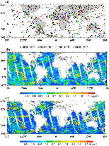Equations to calculate LWP and IWP are (1) $$\begin{array}{c}LW{P}_{\mathit{ECMWF}}=-\frac{1}{g}{\int }_{\mathit{CBP}}^{\mathit{CTP}}{Q}_{\mathit{water}} dp\\ IW{P}_{\mathit{ECMWF}}=-\frac{1}{g}{\int }_{\mathit{CBP}}^{\mathit{CTP}}{Q}_{\mathit{ice}} dp\end{array},$$(1) where Q_water and Q_ice are the liquid water mixing ratio and ice water mixing ratio, respectively, at each model level, and CBP is the cloud-base pressure. For comparisons with model-calculated LWP and IWP, AMSU-A 23.8 and 31.4 GHz channels are used to retrieve the LWP over oceans, and AMSU-B 89 and 150 GHz channels are used to retrieve the IWP (Weng et al., 2003). Figure 1a shows the locations of the selected clear-sky ECMWF profiles (1600 profiles each day), and Fig. 1b shows the geographical distribution of the ECMWF LWP interpolated to NOAA-19 data points over oceans. Lagrange interpolation is used to interpolate in space and time. The black dots show the locations of selected clear-sky ECMWF profiles, which are within three hours of the NOAA-19 data points. The distributions of NOAA-19 AMSU-A-retrieved LWP (Fig. 1c) and ECMWF LWP (Fig. 1b) over oceans are shown, and the retrieved LWPs of at the selected ECMWF clear-sky points, AMSU-A-retrieved LWP values are generally less than 0.05 kg/m², suggesting that the ECMWF determined clear skies are consistent with satellite AMSU-A determined clear skies. The root-mean-square errors of LWP between the two data sources for the 6400 clear-sky ERA-Interim reanalysis profiles within three hours of the NOAA-19 swaths is 0.0018 kg m⁻². The ECMWF clear-sky profiles (black dots) are located mostly in areas that both detect clear skies (see Fig. 5 in Qin and Zou, 2016).

Fig. 1. (a) Geographic distributions of clear-sky ECMWF profiles selected at 0000, 0600, 1200 and 1800 UTC 22 January 2016. (b) Geographical distribution of ECMWF-modelled cloud liquid water path interpolated to NOAA-19 data points, and (c) NOAA-19 AMSU-A-retrieved cloud liquid water path over oceans on 22 January 2016. The black dots in (b) and (c) are a subset of the clear-sky ECMWF profiles selected within three hours of the NOAA-19 data points.

The 399 CrIS channels are applied to channel pairing. The LWIR channels are used to pair SWIR channels based on the following conditions following Lin et al. (2017): (1) The difference between the WF peaks and the lowest cloud-sensitive levels of the LWIR and SWIR channels is less than 80 hPa, and (2) the final pair is selected by choosing the SWIR channel with the smallest standard deviation of simulated brightness temperatures at nadir from the paired LWIR channel over the selected clear-sky ECMWF profiles. Further research into an objective rather than this subjective selection of the 80-hPa threshold is warranted.

The lowest cloud-sensitive level, P_CS, is quantitatively defined by finding the level where the difference between clear-sky and cloudy radiances is less than 1% for the LWIR channels and 10% for the SWIR channels (Lin et al., 2017): (2) $$\begin{array}{c}\Delta R^{\mathit{LWIR}}{|}_{P_{CS}^{\mathit{LWIR}}}=\frac{\left|R_{\mathit{cloudy}}^{\mathit{LWIR}}-R_{\mathit{clear}}^{\mathit{LWIR}}\right|}{R_{\mathit{clear}}^{\mathit{LWIR}}}\le 0.01 \\ \Delta R^{\mathit{SWIR}}{|}_{P_{CS}^{\mathit{SWIR}}}=\frac{\left|R_{\mathit{cloudy}}^{\mathit{SWIR}}-R_{\mathit{clear}}^{\mathit{SWIR}}\right|}{R_{\mathit{clear}}^{\mathit{SWIR}}}\le 0.1\end{array},$$(2) where $R_{\mathit{clear}}^{\mathit{LWIR}}$ and $R_{\mathit{cloudy}}^{\mathit{LWIR}}$ are the clear-sky and cloudy model-simulated radiances, respectively. Table 1 lists the variables used for calculating cloudy radiances with the Community Radiative Transfer Model (CRTM, Version 2.3.0). An overcast ice cloud consisting of particles with an ice water path of 0.05 kg m⁻² is added to one CRTM model level P_L each time to simulate the cloudy radiance. The lowest cloud-sensitive level is the altitude where cloud radiation from the atmosphere below can be ignored. For simulating the clear-sky brightness temperatures of the paired LWIR and SWIR channels, input variables to the CRTM include selected clear-sky ECMWF temperature, specific humidity and ozone profiles, and a constant CO₂ mixing ratio of 390 ppmv. Figure 2 shows the relative ratios of $\Delta R^{\mathit{LWIR}}$ and $\Delta R^{\mathit{SWIR}}$ for LWIR channels 21, 32 and 78 and SWIR channels 349, 342 and 324. The solid and open circles represent the channel-dependent lowest cloud-sensitive levels (see Table 2) for LWIR and SWIR, respectively.

Fig. 2. Relative ratios, $\frac{|R_{\mathit{clear}}-R_{\mathit{cloudy}}|}{R_{\mathit{clear}}},$ for LWIR channels 21, 32 and 78 (solid lines) and SWIR channels 349, 342 and 324 (dashed lines). The vertical grey dotted lines are the thresholds, that is, 0.1 for SWIR and 0.01 for LWIR. The solid and open circles represent the channel-dependent lowest cloud-sensitive levels for LWIR and SWIR, respectively.

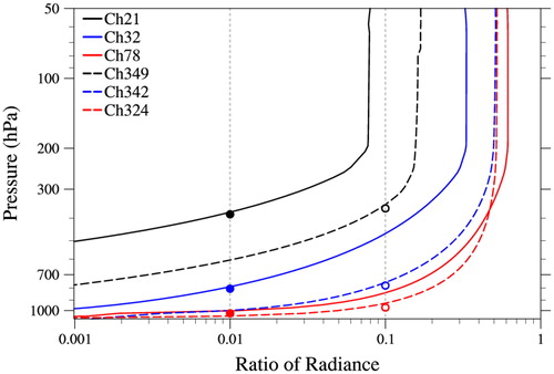
Table 1. Input variables for calculating clear-sky and cloudy radiances with the CRTM.

Category	Variable name	Unit	Data source/assignment
Atmosphere variables	Level and layer pressure	hPa	U.S. standard profile
	Temperature	K
	Water vapour mixing ratio	ppmv
	O3 mixing ratio
	CO2 mixing ratio
	CO mixing ratio
	CH4 mixing ratio
	N2O mixing ratio
Surface variables	Land type	–	Land
	Skin temperature	K	290
	Wind speed	m s^−1	5
	Wind direction	degrees	53
Geometry	Satellite zenith angle	degrees	Observations
Cloud parameters	Cloud type	–	Ice cloud
	Ice water path	kg m^−2	0.05 at each layer

Table 2. Channel number, wave number, weighting function (WF) peaks, and the lowest cloud-sensitive level for 26 paired LWIR and SWIR channels.

	LWIR				SWIR
Pair	Channel number	Wave number (cm^−1)	Peak WF height (hPa)	Cloud insensitive height (hPa)	Channel number	Wave number (cm^−1)	Peak WF height (hPa)	Cloud insensitive height (hPa)
1	6 (37)	672.500	54	54	361 (1206)	2302.500	69	54
2	12 (63)	688.750	69	64	360 (1204)	2297.500	80	54
3	19 (75)	696.250	156	307	351 (1193)	2252.500	156	293
4	22 (81)	700.000	175	367	350 (1192)	2267.500	156	321
5	21 (80)	699.375	229	416	349 (1190)	2262.500	185	383
6	23 (83)	701.250	254	416	348 (1189)	2260.000	218	416
7	37 (111)	718.750	321	545	347 (1187)	2242.500	307	586
8	55 (147)	741.250	433	790	343 (1178)	2232.500	367	840
9	32 (101)	712.500	487	815	342 (1177)	2230.000	416	892
10	36 (107)	716.250	565	918	337 (1171)	2215.000	525	945
11	39 (116)	721.875	650	945	334 (1168)	2207.500	628	945
12	59 (153)	745.000	742	945	332 (1166)	2202.500	718	972
13	72 (168)	754.375	766	1000	341 (1175)	2225.000	742	972
14	60 (154)	745.625	840	1000	340 (1174)	2222.500	790	972
15	57 (150)	743.125	892	1000	329 (1163)	2195.000	866	1000
16	82 (216)	784.375	945	1028	326 (1160)	2187.500	972	1000
17	73 (170)	755.625	1000	1057	387 (1244)	2397.500	1000	1057
18	74 (171)	756.250	1057	1057	388 (1245)	2400.000	1028	1028
19	78 (183)	763.750	1085	1000	324 (1158)	2182.500	1085	1028
20	79 (198)	773.125	1085	1000	323 (1157)	2180.000	1085	1028
21	97 (334)	858.125	1085	1028	320 (1154)	2172.500	1085	1028
22	122 (447)	928.750	1085	1028	321 (1155)	2425.000	1085	1000
23	123 (464)	939.375	1085	1000	319 (1153)	2170.000	1085	1028
24	133 (561)	1000.000	1085	1000	327 (1161)	2175.000	1085	1028
25	136 (565)	1007.500	1085	1000	328 (1162)	2177.500	1085	1028
26	183 (710)	1093.125	1085	1000	322 (1156)	2427.500	1085	1028

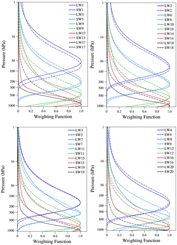
Figure 3 shows the WF peaks and the lowest cloud-sensitive levels of the 399 CrIS channels for NWP. The different gas absorption bands are also shown. A total of 26 LWIR and SWIR channels are finally paired. Table 2 lists the channel number, wave number, WF peak and the lowest cloud-sensitive level of the 26 paired LWIR and SWIR channels. Figure 4 shows the WFs of the paired LWIR and SWIR channels. The paired LWIR and SWIR channels have nearly coincident WF peaks and similar vertical distributions. Temperature and cloud information at different atmospheric levels can thus be monitored effectively. The WFs have been normalised and are non-dimensional in this study.

Fig. 3. Weighting function peaks (black) and the lowest cloud-sensitive levels (red) of the 399 CrIS channels selected for NWP, calculated using the CRTM with the U.S. standard atmosphere profile.

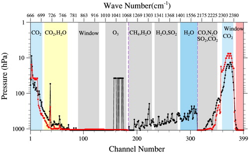
Fig. 4. Normalised weighting functions for the LWIR (solid lines) and SWIR (dashed lines) channels of pairs 1–20.

3.2. Definition and bias corrections of the cloud emission and scattering index (CESI)

A linear model of clear-sky brightness temperature between each paired LWIR and SWIR channel is developed as follows: (3) $$T_{b,i,\mathit{regression}}^{SW}={\alpha }_i\cdot T_{b,i}^{LW}+{\beta }_i,$$(3) where the subscript i represents the pair number. The parameters ${\alpha }_i$ and ${\beta }_i$ are regression coefficients, obtained by the least-squares method: (4) $$\{\begin{array}{l}{\alpha }_i=\frac{\sum _{j=1}^N(T_{b,i}^{SW}(j)-\overline{T_{b,i,\mathit{regression}}^{SW}})(T_{b,i}^{LW}(j)-\overline{T_{b,i}^{LW}})}{\sum _{j=1}^N{(T_{b,i}^{LW}-\overline{T_{b,i}^{LW}})}^2}\\ {\beta }_i=\overline{T_{b,i,\mathit{regression}}^{SW}}-{\alpha }_i\overline{T_{b,i}^{LW}}\end{array},$$(4) where the subscript j represents the clear-sky ECMWF profile number, and N is the total number of samples. The simulated clear-sky brightness temperatures of the middle FOV (pixel 5) is used to calculate the regression coefficients.

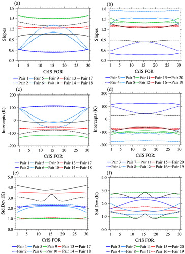
Figure 5 shows data count of CRTM-simulated brightness temperatures at CrIS observation pixel locations of FORs 1and 15 for pairs 9 (LWIR channel 32, SWIR channel 342) and 19 (LWIR channel 78, SWIR channel 324). The brightness temperatures of the paired LWIR and SWIR channels are strongly correlated under clear-sky conditions with correlation coefficients greater than 0.96. The slopes of the fitting lines for different FORs are different, so it is necessary to obtain regression coefficients for different FORs. Figure 6 shows the slopes, intercepts, and standard deviations of the regression model for FORs 1–30 of the pairs 1–20. The slopes and intercepts are almost symmetric about FOR 15 (nadir). The model standard deviations are less than 3 K, which suggests a strong linear relationship.

Fig. 5. Data count of CRTM-simulated brightness temperatures of (a, b) pair-9 channels and (c, d) pair-19 channels at the field of regards (FORs) 15 (left panels) and 1 (right panels) using the 6400 selected clear-sky ECMWF profiles. The letter ‘R’ represents the correlation coefficient.

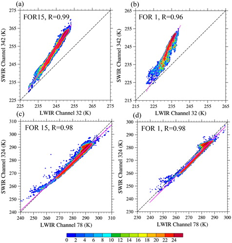
Fig. 6. Regression coefficients (a, b) α and (c, d) β, and (e, f) standard deviations of the regression model$(T_{b,\mathit{regression}}^{\mathit{SWIR}}-T_{b,\mathit{CRTMclear}}^{\mathit{SWIR}})$ for 30 fields of regard (FORs) of pairs 1–20.

The CESI can finally be defined as the difference between the SWIR-observed brightness temperature and the linear-regression-estimated SWIR brightness temperature: (5) $$\mathit{CES}{I}_i=T_{b,i,\mathit{obs}}^{SW}-T_{b,i,\mathit{regression}}^{SW}=T_{b,i,\mathit{obs}}^{SW}-({\alpha }_i{T}_{b,i,\mathit{obs}}^{LW}+{\beta }_i).$$(5)

The brightness temperatures of the LWIR and SWIR channels are likely very low near optically thick ice clouds (ice cloud optical depth, ICOD > 1), but the SWIR brightness temperatures are several degrees warmer than the LWIR brightness temperatures due to different cloud infrared emissions, suggesting different responses to the presence of optically thick ice clouds. The linear relationship between the paired channels under clear-sky conditions will be violated in cloudy conditions. Therefore, the CESI of different layers in the atmosphere can be used to identify ice clouds located in different layers of the atmosphere.

The latitudinal and scan-dependent biases of CESIs require quantification due to the thermal differences between latitudes and the limb effect of cross-track instruments like CrIS. Figure 9 also shows the latitudinal and scan-dependent biases seen in the spatial distribution of pair 9’s CESI (CESI-9).

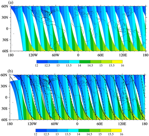
AIRS v6 cloud products are applied to estimate the latitudinal and scan-dependent biases and validate the derived CESIs. The AIRS has the same equator crossing local time as the CrIS, which is 13:30 pm at their ascending nodes. Their orbit heights and cycles, however, are different, so their orbital tracks are different. Figure 7 shows the distributions of the local time of the AIRS and the CrIS on 22 January 2016. The conversion relationship between UTC and Local Standard Time (LST) is (6) $${\mathit{LST}}_{(\lambda ,\phi )}={UTC}_{(\lambda ,\phi )}\pm \left|\lambda \right| /15,$$(6) where λ and φ represent the latitude and longitude, respectively. When λ > 0, the plus sign is used, and when λ < 0, the minus sign is used. The LSTs of the CrIS and the AIRS are close when passing over the same regions. Since the two satellites carrying these instruments follow each other, large amounts of overlapping CrIS and AIRS data can be obtained. The CrIS data points are collocated with the closest AIRS data points within three hours to constitute the CrIS-AIRS dataset that includes latitude, longitude, CESI and AIRS v6 cloud products.

Fig. 7. Local time distributions (unit: hour) of (a) the AIRS and (b) the CrIS from ascending nodes during 0300–2400 UTC 22 January 2016. The black lines in (b) are the limb along-tracks of the AIRS.

Clear-sky (ECA = 0) CrIS-AIRS data from 15–21 January 2016 are selected to estimate the latitudinal mean bias $\mu ({\phi }_j)=\overline{\mathit{CES}{I}_j^{\mathit{for}15}}-\overline{\mathit{CES}{I}_{\mathit{\text{a\hspace{0.05em}ll\hspace{0.05em}\hspace{0.05em}}}\mathit{bands} }^{\mathit{for}15}}$ and the scan-dependent bias $\mu ({\alpha }_i)=\overline{\mathit{CES}{I}_i\mathit{CES}{I}_{\mathit{for}15}}.$ Finally, the CESI after bias corrections is defined as (7) $$\mathit{CES}{I}_{\mathit{after}}=\mathit{CES}{I}_{\mathit{before}}-\mu (\phi )-\mu (\alpha ),$$(7) where i represents the FORs 1–30, and j represents latitude bands 1–24 (5° each band from 60°S to 60°N). Figure 8 shows latitudinal- and scan-dependent biases for CESI-5, CESI-9 and CESI-19 at ascending and descending nodes in January, April, July and October 2016. The latitudinal dependence of biases for the surface CESI-19 has a clear seasonal variability due to surface effects. The scan-dependent biases are relatively stable for all three CESIs. Figure 9 shows the spatial distributions of CESI-9 (452 hPa) without (Fig. 9a) and with (Fig. 9b) bias corrections as well as the differences between Fig. 9(a) and Fig. 9(b) at CrIS ascending nodes on 22 January 2016. Results suggest an effective elimination of the scan dependence of CESI-9. The latitudinal and scan-dependent biases are reduced after bias correction, making the distribution of optically thick clouds more clearly seen. Figure 10 shows the spatial distributions of AIRS v6 ICOD and the corresponding CESI-19 (1085 hPa) between 60°S and 60°N for the ascending (daytime) node on 22 January 2016. The distributions of CESI-19 and ICOD are generally consistent.

Fig. 8. (a–d) Latitudinal biases for CESI-5 (black), CESI-9 (blue), and CESI-19 (red) using the nadir FOR 15. (e–h) Differences in mean CESI between non-nadir FORs and the nadir FOR 15, taken as the scan-angle correction. Data are the clear-sky AIRS-CrIS overlapped ascending (solid lines) and descending (dashed lines) data points between 60°S and 60°N from 15–21 January, 15–21 April, 15–21 July and 15–21 October 2016.

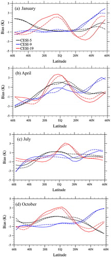
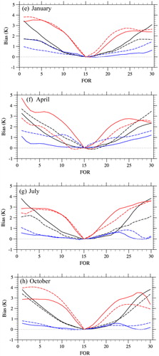
Fig. 9. Spatial distributions of CESI-9 (a) without and (b) with bias correction at CrIS ascending nodes on 22 January 2016. (c) Differences between (a) and (b).

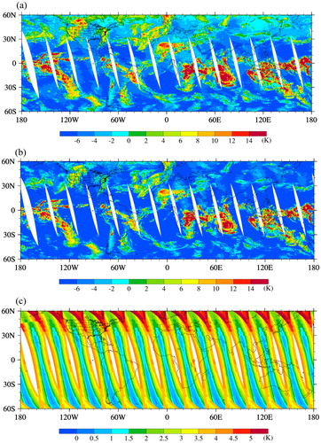
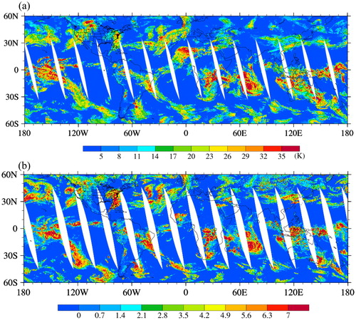
Fig. 10. Spatial distributions of (a) CESI-19 and (b) AIRS version 6 ice cloud optical thickness from ascending nodes between 60°S and 60°N on 22 January 2016.

4. Validation of the CESI

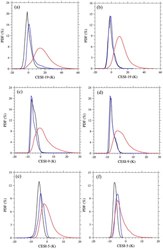
The purpose of this study is to estimate the cloud-top heights of ice clouds using the derived CESI for different layers. The indices, CESI-16 to CESI–26 whose weighting function peaks are located at and near the surface (see Table 2), shall be affected by ice clouds located at all atmospheric levels. CESI-19 will be used as an example to demonstrate this. Thresholds can then be determined to identify ice clouds. Figure 11 shows the daytime and nighttime probability distributions of CESI-19, CESI-9 and CESI-5 when clear skies, water clouds and ice clouds are present using data on 22 January 2016. The CESI-19 is most sensitive to ice clouds, less sensitive to water clouds and is insensitive to clear skies. The distributions of ice clouds for CESI-9 and CESI-5 are closer to those of clear skies and water clouds since low-level ice clouds do not affect middle- and high-level indices CESI-9 and CESI-5.

Fig. 11. Probability distributions of (a, b) CESI-19, (c, d) CESI-9, and (e, f) CESI-5 under clear skies (black), water clouds (blue) and ice clouds (red) from AIRS-CrIS overlapped data points between 60°S and 60°N at ascending (left panels) and descending (right panels) nodes on 22 January 2016.

CESI-19 and ICOD are compared and evaluated using the probability of correct typing (PCT), the false alarm rate (FAR), the leakage rate (LR) and the Heike skill score (HSS), defined as follows (Zhuge and Zou, 2016): (9) $$\mathit{PCT}=\frac{N(T_{\mathit{cld}}\cap C_{\mathit{cld}}+T_{\mathit{clr}}\cap C_{\mathit{clr}})}{N(T_{\mathit{cld}}+T_{\mathit{clr}})},$$(9) (10) $$\mathit{FAR}=\frac{N(T_{\mathit{clr}}\cap C_{\mathit{cld}})}{N(T_{\mathit{cld}}+T_{\mathit{clr}})},$$(10) (11) $$LR=\frac{N(T_{\mathit{cld}}\cap C_{\mathit{clr}})}{N(T_{\mathit{cld}}+T_{\mathit{clr}})},$$(11) (12) $$\mathit{HSS}=\frac{N(T_{\mathit{cld}}\cap C_{\mathit{cld}}+T_{\mathit{clr}}\cap C{}_{\mathit{clr}})-\frac{N(T_{\mathit{cld}})N(C_{\mathit{cld}})+N(T_{\mathit{clr}})N(C_{\mathit{clr}})}{N(T_{\mathit{cld}}+T_{\mathit{clr}})}}{N(T_{\mathit{cld}}+T_{\mathit{clr}})-\frac{N(T_{\mathit{cld}})N(C_{\mathit{cld}})+N(T_{\mathit{clr}})N(C{}_{\mathit{clr}})}{N(T_{\mathit{cld}}+T_{\mathit{clr}})}},$$(12) where $T_{\mathit{cld}}$ and $T_{\mathit{clr}}$ stand for the true ice clouds (ICOD > 0) and non-ice clouds (ICOD = 0) data points; $C_{\mathit{cld}}$ and $C_{\mathit{clr}}$ represent the ice clouds and non-ice clouds data points, respectively, based on the CESI-19 threshold.

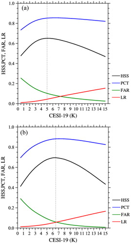
Figure 12 shows the PCT, FAR, LR, and HSS of CESI-19 and ICOD where ‘true’ data are ICOD data. A good cloud detection method should have high PCT and HSS values but low FAR and LR values. We use the maximum value of HSS to determine the threshold of CESI-19. PCT, FAR, LR and HSS are 85.3%, 9.5%, 4.5% and 0.65, respectively, when the daytime CESI-19 is set to 5 K (Fig. 14a) and 86.5%, 5.1%, 5.0% and 0.68, respectively, when the nighttime CESI-19 is set to 6.5 K (Fig. 14b).

Fig. 12. The probabilities of correct typing (PCT, blue), the false alarm rate (FAR, green), the leakage rate (LR, red), and the Heike skill score (HSS, black) of different thresholds of CESI-19 and ICOD from (a) ascending and (b) descending nodes on 22 January 2016. ‘True’ data are ICOD data. The black dotted line is set at the maximum HSS value.

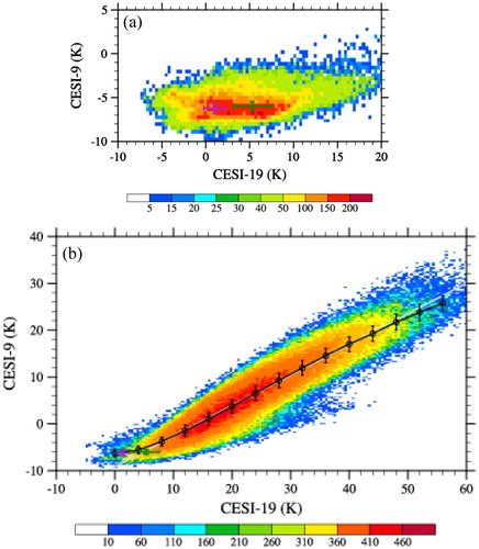
The distribution of clear-sky CESIs is first examined to determine the CESI-5 and CESI-9 thresholds for ice clouds. The average values of CESI-5, CESI-9 and CESI-19 under clear-sky conditions are −4.0 K, −6.2 K and 2.4 K, respectively. Figure 13a shows CESI-19 and CESI-5 data counts when ICOD > 0 and CTP > 300 hPa. The average value of CESI-5 is almost the same as that under clear-sky conditions, suggesting that CESI-5 is insensitive to ice clouds with CTPs > 300 hPa. However, the mean value of CESI-19 increases from 2.4 K to 12 K in the presence of ice clouds with CTPs > 300 hPa. Figure 13b shows CESI-19 and CESI-5 data counts when ICOD > 0 and CTP $\le$ 300 hPa. Both CESI-5 and CESI-19 are sensitive to ice clouds with a linear slope of 0.22, indicating that CESI-5 is sensitive to ice clouds with CTPs ≤ 300 hPa. Figure 14 shows CESI-19 and CESI-9 data counts when ICOD > 0, CTP > 600 hPa and ICOD > 0, CTP$\le$600 hPa. The mean value of CESI-9 is the same as that under clear-sky conditions, suggesting that CESI-9 is insensitive to ice clouds with CTPs $\le$ 600 hPa. When CTP $\le$ 600 hPa, both CESI-9 and CESI-19 are sensitive to ice clouds with a linear slope reaching 0.62.

Fig. 13. CESI-19 and CESI-5 data counts (bin size: 0.5 K × 0.25 K) when (a) ICOD > 0, CTP > 300 hPa, and (b) ICOD > 0, CTP$\le \mathrm{}$300 hPa. The crosses are the means and standard deviations of the CESIs of the coordinate axes under clear-sky (purple) and ICOD > 0, CTP > 300 hPa (green) conditions. The black curves connect the means (black dots) and standard deviations (vertical lines) of CESI-5 in each CESI-19 4-K bin (x-axis). AIRS-overlapped CrIS data points between 60°S and 60°N from the ascending swaths during 23–28 January 2016 are used.

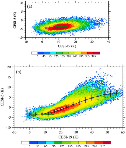
Fig. 14. Same as Fig. 13 except for CESI-19 and CESI-9 data counts when (a) ICOD > 0, CTP > 600 hPa, and (b) ICOD > 0, CTP$\le \mathrm{}$600 hPa. The crosses are the means and standard deviations of the CESIs of the coordinate axes under clear-sky (purple) and ICOD > 0, CTP > 600 hPa (green) conditions.

Figure 15 shows the HSS and PCT for both the CESI-5 (Fig. 15(a) and CESI-9 (Fig. 15(b)). Since the weighting functions of the two SWIR and LWIR channels of this cloud index CESI-5 peak around 200 hPa, we examine how CESI-5 detects the clouds detect clouds with the CTP varying from 400 to 100 hPa. It is found that the maximum HSS is located at CESI-5 = −3 K and CTP = 220 hPa. In other words, CESI-5 > −3 K best detect those ice clouds with cloud tops above the 220-hPa level. For the HSS and PCT calculations for the CESI-9 (Fig. 15(b)), data satisfying CESI-5 $\le$ −3 K are not included since they are detected as cloudy by the CESI-5. The maximum HSS is located at (−1 K, 390 hPa). Therefore, ice clouds whose cloud tops are above the 390-hPa level can be identified by CESI-9 > −1 K. Super Typhoon Maria occurred over the Western Pacific in July 2018. Figures 16a–c show the spatial structures of CESI-5, 9, and 19 at 0417 UTC 9 July 2018 at the CrIS ascending node. The CESIs all reveal Typhoon Maria’s eye, eyewall and rainbands. When CESI-5 > −3 K and CESI-9 > −1 K, the CTPs of ice clouds can reach above 200 hPa and 400 hPa, respectively (Fig. 17e). This is consistent with the AIRS v6 CTPs (Fig. 16f).

Fig. 15. (a) The Heike skill score (color shading), probability of correct typing (black lines) for the (a) CESI-5 with the cloud top pressure of ice clouds and (b) CESI-9 with cloud top pressure of ice clouds under condition of CESI-5$\le$−3 K from ascending nodes during 22 January 2016. The black dashed lines represent the maximum Heike skill score locations (a) (−3 K, 220 hPa) and (b) (−1 K, 390 hPa).

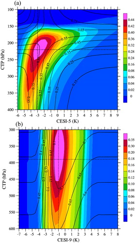
Fig. 16. Spatial distributions of (a) CESI-5, (b) CESI-9, (c) CESI-19 and (d) AIRS ICOD for Typhoon Maria at 0417 UTC 9 July 2018 at the ascending node. (e) CESI-5 > −3 K (blue, ice cloud above 200 hPa), CESI-9 > −1 K (green, ice cloud between 200 and 400 hPa), CESI-19 > 5 K (red, ice or liquid cloud below 400 hPa), and CESI-19 $\le$ 5 K (grey, clear sky) from the AIRS-CrIS overlapped swath. (f) Cloud-top pressures are from AIRS v6 product. The black lines in (a–f) show the track of the Cloud-Aerosol Lidar with Orthogonal Polarization onboard the Cloud-Aerosol Lidar and Infrared Pathfinder Satellite Observation satellite.

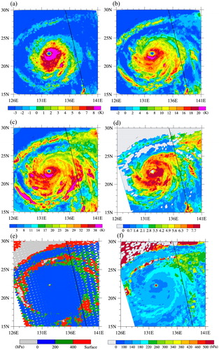
Fig. 17. The vertical distributions of (a) ice water content (unit: g m⁻³) and (b) cloud fraction along the CALIOP track shown in Fig. 16.

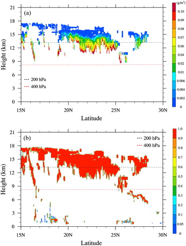
Figure 17 shows the vertical distributions of ice water content (Fig. 17a) and cloud fraction (Fig. 17b) along the track of the Cloud-Aerosol Lidar with Orthogonal Polarization (CALIOP) onboard the Cloud-Aerosol Lidar and Infrared Pathfinder Satellite Observation satellite’s ascending node on 9 July 2018 (see Figure 16). The geographic locations of high clouds, middle clouds (16°N–16.5°N, 25.2°N–26.3°N) and low clouds or clear sky (28°N–30°N) in Figure 17 are consistent with the CESI results shown in Figures 16a–c,e.

5. Summary and conclusions

NWP models have commonly used observations from the CrIS onboard the S-NPP satellite, which contain a large amount of information regarding high-resolution atmosphere temperature and water vapour profiles. This study presents a new method to detect ice clouds located at different altitudes using the CESIs derived from paired CrIS LWIR and SWIR channels. The CESIs can better reflect the ice cloud distributions after bias corrections. Three CESIs in particular, that is, CESI-5, −9 and −19, can well detect clouds located above 200 hPa, between 200 and 400 hPa, and below 400 hPa, respectively, when the thresholds are set to around −3 K, −1 K and 5 K, respectively. By comparing the AIRS v6 ICOD and CTP products, the 5-K (6.5-K) CESI-19 threshold during the daytime (nighttime) gives a PCT of ∼85.3% (86.5%), a FAR of 9.5% (5.1%), an LR of 4.5% (5.0%) and an HSS of 0.65 (0.68), suggesting reasonable cloud detection results. The horizontal spatial distributions of CESI-5, CESI-9 and CESI-19 within Typhoon Maria at 0417 UTC 9 July 2018 compared favourably with the horizontal spatial distributions of AIRS ICOD and CTP, as well as the vertical distributions of CALIOP’s ice water content and cloud fraction retrievals.

In the future, thresholds of all pairs of CESIs will be determined to detect clouds with different cloud top pressures, and their performances will be evaluated. CrIS channels above a certain altitude can, therefore, be removed or retained based on the channel-dependent cloud-sensitive level and the threshold of a CESI. This physically based method of cloud detection would significantly increase the number of useable CrIS clear-channel radiances for satellite data assimilation. Validating CESIs using collocated observations from the CrIS and the CALIOP is also feasible.

Additional information

Funding

This research was supported by the National Key R&D Program of China (Grant 2018YFC1506702) and the National Natural Science Foundation of China Grant 91337218.

References

- Carrier, M., Zou, X. and Lapenta, W. M. 2007. Identifying cloud-uncontaminated AIRS spectra from cloudy FOV-based on cloud-top pressure and weighting functions. Mon. Wea. Rev. 135, 2278–2294. doi:10.1175/MWR3384.1
- Collard, A. D. 2004. Assimilation of AIRS observations at the Met Office. In: Proceedings of the Workshop on Assimilation of High Spectral Resolution Sounders in NWP, Reading, UK, ECMWF, pp. 63–71.
- Dee, D. P. 2005. Bias and data assimilation. Q. J. R. Meteorol. Soc. 131, 3323–3343. doi:10.1256/qj.05.137
- Eyre, J. R. and Watts, P. 2007. A sequential estimation approach to cloud-clearing for satellite temperature sounding. Q. J. R. Meteorol. Soc. 113, 1349–1376. doi:10.1002/qj.49711347814
- Gambacorta, A. and Barnet, C. D. 2013. Methodology and information content of the NOAA NESDIS operational channel selection for the cross-track infrared sounder (CrIS). IEEE Trans. Geosci. Remote Sens. 51, 3207–3216. doi:10.1109/TGRS.2012.2220369
- Goldberg, M. D., Qu, Y., McMillin, L. M., Wolf, W. and Zhou, L. and co-authors 2003. AIRS near-real-time products and algorithms in support of operational numerical weather prediction. IEEE Trans. Geosci. Remote Sens. 41, 379–389. doi:10.1109/TGRS.2002.808307
- Han, Y., Revercomb, H., Cromp, M., Gu, D., Johnson, D. and co-authors. 2013. Suomi NPP CrIS measurements, sensor data record algorithm, calibration and validation activities, and record data quality. J. Geophys. Res. Atmos. 118, 12,734–12,748. doi:10.1002/2013JD020344
- Han, Y., Zou, X. and Weng, F. 2015. Cloud and precipitation features of Super Typhoon Neoguri revealed from dual oxygen absorption band sounding instruments on board FengYun-3C satellite. Geophys. Res. Lett. 42, 916–924. doi:10.1002/2014GL062753
- Kahn, B. H., Irion, F. W., Dang, V. T., Manning, E. M., Nasiri, S. L. and co-authors. 2014. The atmospheric infrared sounder version 6 cloud products. Atmos. Chem. Phys. 14, 399–426. doi:10.5194/acp-14-399-2014
- Li, X., Zou, X. and Zeng, M. 2019. An alternative bias correction scheme for CrIS data assimilation in regional model. Mon. Wea. Rev. 147, 809–839. doi:10.1175/MWR-D-18-0044.1
- Liang, D. and Weng, F. Z. 2014. Evaluation of the impact of a new quality control method on assimilation of CrIS data in HWRF-GSI. In: Proceedings of the IEEE Geoscience and Remote Sensing Symposium, Québec City, QC, Canada, pp. 3778–3781.
- Lin, L., Zou, X. and Weng, F. Z. 2017. Combining CrIS double CO2 bands for detecting clouds located in different vertical layers of the atmosphere. J. Geophys. Res. Atmos. 122, 1811–1827. doi:10.1002/2016JD025505
- McNally, A. P. and Watts, P. D. 2003. A cloud detection algorithm for high-spectral-resolution infrared sounders. Q. J. R. Meteorol. Soc. 129, 3411–3423. doi:10.1256/qj.02.208
- Menzel, W., Smith, T. and Stewart, T. R. 1983. Improved cloud motion wind vector and altitude assignment using VAS. J. Clim. Appl. Meteor. 22, 377–384. doi:10.1175/1520-0450(1983)022<0377:ICMWVA>2.0.CO;2
- Pavelin, E., English, S. and Eyre, J. 2008. The assimilation of cloud-affected infrared satellite radiances for numerical weather prediction. Q. J. R. Meteorol. Soc. 134, 737–749. doi:10.1002/qj.243
- Qin, Z. and Zou, X. 2016. Uncertainty in Fengyun-3C microwave humidity sounder measurements at 118 GHz with respect to simulations from GPS RO data. IEEE Trans. Geosci. Remote Sens. 54, 6907–6918. doi:10.1109/TGRS.2016.2587878
- Spankuch, D. and Döhler, W. 1985. Radiative properties of cirrus clouds in the middle IR derived from Fourier spectrometer measurements from space. Z. Meteorol. 35, 314–324.
- Weng, F., Zhao, L., Ferraro, R., Poe, G., Li, X. and co-authors. 2003. Advanced microwave sounding unit cloud and precipitation algorithms. Radio Sci. 38, 86–96.
- Zhuge, X. and Zou, X. 2016. Test of a modified infrared only ABI cloud mask algorithm for AHI radiance observations. J. Appl. Meteor. Climatol. 55, 2529–2546. doi:10.1175/JAMC-D-16-0254.1