Probabilistic thunderstorm forecasting by blending multiple ensembles

Abstract

In numerical weather prediction models, point thunderstorm forecasts tend to have little predictive value beyond a few hours. Thunderstorms are difficult to predict due largely to their typically small size and correspondingly limited intrinsic predictability. We present an algorithm that predicts the probability of thunderstorm occurrence by blending multiple ensemble predictions. It combines several post-processing steps: spatial neighbourhood smoothing, dressing of probability density functions, adjusting sensitivity to model output, ensemble weighting, and calibration of the output probabilities. These operators are tuned using a machine learning technique that optimizes forecast value measured by event detection and false alarm rates. An evaluation during summer 2018 over western Europe demonstrates that the method can be deployed using about a month of historical data. Post-processed thunderstorm probabilities are substantially better than raw ensemble output. Forecast ranges from 9 hours to 4 days are studied using four ensembles: a three-member lagged ensemble, a 12-member non-lagged limited area ensemble, and two global ensembles including the recently implemented ECMWF thunderstorm diagnostic. The ensembles are combined in order to produce forecasts at all ranges. In most tested configurations, the combination of two ensembles outperforms single-ensemble output. The performance of the combination is degraded if one of the ensembles used is much worse than the other. These results provide measures of thunderstorm predictability in terms of effective resolution, diurnal variability and maximum forecast horizon.

Keywords:

• thunderstorm
• numerical weather prediction
• ensemble prediction
• probabilistic weather forecasts
• surrogate model

1. Introduction

Despite the sophistication of current operational numerical weather prediction systems, thunderstorms remain relatively unpredictable at fine scales beyond a few hours (Clark et al., 2009). Most modern numerical atmospheric models can simulate key physical features of deep convective systems that produce thunderstorms, either by implicitly modelling subgrid convection in large scale models, or by explicitly resolving 3D convective clouds in non-hydrostatic models at kilometric resolutions. A discussion of the merits of both approaches is provided in Weisman et al. (2008). Beside the limited realism of numerical models, thunderstorm prediction is hampered by the usually poor predictability of deep convective clouds (Walser et al., 2004): rapid error growth in the simulation of convective systems can lead to large uncertainties in their location, timing and intensity. Thunderstorm predictability has been shown to depend on the meteorological context, for instance ‘air mass’ (i.e. weakly forced) convection tends to be less predictable than synoptically forced events (Keil et al., 2014). Sobash et al. (2011) explored storm risk ensemble predictions using spatial smoothing to account for location errors. Several authors have proposed lightning risk diagnostics for numerical model output, but the published results have so far been restricted to relatively large spatial and temporal scales due to the high forecast uncertainty (e.g. Casati and Wilson, 2007; Schmeits et al., 2008; Yair et al., 2010; Collins and Tissot, 2015; Gijben et al., 2017; Simon et al., 2018).

Ensemble prediction can help users interpret highly uncertain weather forecasts (Richardson, 2000; Zhu et al., 2002). Ensembles simulate the real-time propagation of uncertainties in the prediction process: pseudo-random error structures called perturbations are injected into the numerical weather prediction systems. Perturbations include some representation of uncertainties in the initial conditions (e.g. Descamps and Talagrand, 2007) and in the model design (see review in Leutbecher et al., 2017). Using a perturbation sample, a set of forecasts called ensemble members is computed in real time to simulate the probability distribution of uncertainties in the forecast products. The size of current operational ensembles (typically 10–50 members) is a compromise between model realism and statistical accuracy under the constraint of affordable computing cost. This size is arguably much smaller than the ensemble size needed to properly sample the space spanned by forecast errors (Leutbecher, 2018). In some applications, the ensemble size can be increased by including older predictions into the product generation (Lu et al., 2007; Osinski and Bouttier, 2018).

In single-model ensembles, the implementation of perturbation schemes can be constrained by the architecture of the numerical models and data assimilations used. A possible workaround is to mix multiple physics packages, multiple models or multiple ensembles in the member generation (e.g. Ziehmann, 2000; Clark et al., 2008; Park et al., 2008; Hagedorn et al., 2012). These approaches have been shown to provide benefits, although they could possibly be superseded one day by single-model ensembles thanks to ongoing research to improve perturbation schemes.

Ensembles are limited by our ability to represent error sources in the initial conditions and model design, because the perturbation setup is always constrained by the architecture of the numerical models and data assimilations used. This issue can be somewhat alleviated by mixing multiple physics packages, multiple models or multiple ensembles in the member generation (e.g. Ziehmann, 2000; Clark et al., 2008; Park et al., 2008; Hagedorn et al., 2012).

An important application of ensemble prediction is point probabilistic forecasts, i.e. real time estimation of the likelihood of future meteorological events, at predefined locations in space and time. These forecasts can be verified a posteriori using a variety of statistical measures such as reliability and resolution (Jolliffe and Stephenson, 2011). Ultimately, the usefulness of probabilistic forecasts depends on the user. Here, we will focus on binary forecasts of a particular meteorological event: thunderstorm occurrence. Its quality will be measured using the frequency of non-detections and false alarms, as summarized by the ROC diagram (relative operating characteristic, Mason and Graham, 1999) averaged over many point forecasts. Other, more user-specific scores could be used, such as the potential economic value (Richardson, 2000).

Various ensemble post-processing techniques have been proposed to improve probabilistic forecasts using historical data: dressing (Bröcker and Smith, 2008), Bayesian model averaging (Raftery et al., 2005; Berrocal et al., 2007), ensemble model output statistics (EMOS, Gneiting et al., 2005), random forest quantiles (Taillardat et al., 2016), among others. Simon et al. (2018) presented a statistical thunderstorm forecasting technique based on a generalized additive model (GAM) algorithm. These techniques tend to require large homogeneous learning datasets, which may be difficult to obtain for rare events. In most weather centres, model upgrades occur frequently (at least annually), in which case the learning datasets have to be updated using potentially expensive reforecast techniques (Hamill et al., 2006, 2008). This can be problematic in a production setting that uses model output from several weather centres, each upgrading their own systems on independent schedules.

This paper presents an original technique for point probabilistic thunderstorm forecasts,. It deals with the above issues by combining multiple ensembles with a simple calibration technique. Our goal is to check if the end user value of ensembles can be improved by calibrating their output, using techniques that require little learning data. We will combine the following post-processing operators: each is relatively well known, but they have to our knowledge not yet been integrated as a single algorithm:

• a neighbourhood operator that allows for some spatial tolerance in the use of model-generated thunderstorms, following the ideas of Theis et al. (2005), Berrocal et al. (2007) and Schwartz and Sobash (2017);

• a kernel dressing in order to smooth the ensemble probability distribution function (PDF) in parameter space (Berrocal et al., 2007; Bröcker and Smith, 2008);

• a calibration of the model diagnostic used to define the occurrence of thunderstorms: we use a much simplified version of existing calibration techniques (e.g. Gneiting et al., 2005; Ben Bouallègue, 2013; Simon et al., 2018), which can be understood as a bias correction of the modelled thunderstorm intensity;

• an optimal weighting of the ensembles that are combined to produce the thunderstorm forecasts, which brings model diversity into the e190924thunprob-revised.pdfnd products (see e.g. Hagedorn et al., 2012; Beck et al., 2016).

As explained below, these operators involve tuning parameters that will be optimized in terms of forecast error statistics (i.e. thunderstorm non-detection and false alarms rates), while requiring that forecast probabilities be reasonably well calibrated. We will demonstrate the performance of the results on several combinations of ensemble prediction systems that cover a wide range of forecast horizons, from a few hours to several days. The paper is organised as follows: the observations and ensemble forecasts are presented in Section 2. The parameter tuning procedure is explained in Section 3, and its variability is explored in Section 4. The performance of the optimized forecasts is studied in Section 5, before the discussion and concluding remarks in Section 6.

2. Observation and forecast data

2.1. Thunderstorm observations

In this paper, we regard thunderstorm occurrence as a binary field, without consideration of event intensity. Different users may be sensitive to different aspects of thunderstorm activity, such as heavy accumulation, hail, gusts, cloud-to-ground lightning strikes, etc. Thus, there are several possible ways of defining thunderstorm observations. In this work we use lightning sensors and radar reflectivities to define thunderstorms observations, because these measurements are readily available over our domain of interest, in Western Europe. The lightning data is provided by the Météorage company, based on LS700X Vaisala sensors, with some filtering to eliminate non-meteorological signals. After data processing, the reported detection rate in this area is of the order of 90% for cloud-to-ground strikes, and 50% for intracloud strikes (Pédeboy and Schulz, 2014). The radar data is provided by the Météo-France PANTHERE network of ground-based polarimetric radars, which is designed to provide good coverage over mainland France and Corsica. Depending on their development stage, thunderstorm clouds can affect much larger zones than their electrically active areas; conversely, thunderstorms can have significant lightning activity but little precipitation. Some mostly produce intracloud flashes that are imperfectly detected by the lightning sensors. We combine lightning and radar data as explained below, in order to minimize the impact of these complexities on the verification. In regions without these observing systems, satellite based data could be used, such as cloud-top diagnostics (Karagiannidis et al., 2019) or optical lightning sensors (Goodman et al., 2013).

We are interested in predicting thunderstorm impacts at the hourly scale, with a resolution of a few kilometres: a thunderstorm will be deemed to occur if a lightning strike is observed within 10 km and 30 min of the observation, or the maximum radar reflectivity in this neighbourhood is greater than 35dBZ (this threshold is commonly used for radar thunderstorm detection; see Li et al. (2012) and references therein). This criterion is applied at all full hours and on each point of a regular latitude-longitude grid of 20 km mesh, in order to generate a set of pseudo-observations. Forecast verification will be performed on the domain represented in Fig. 1. There are 1748 pseudo-observations at each hour i.e. about 1.3 million data points per month. The period studied here is June to August 2018, during which thunderstorm activity was observed at 2% of the data points. An example of thunderstorm pseudo-observation coverage is presented in Fig. 1.

2.2. Numerical model forecasts

We investigate the predictive value of four ensemble prediction systems, selected for a typical user that requires forecasts over Europe in the early morning (around 04UTC). Their timings are summarized in Fig. 2.

The lagged Arome ensemble (named AROLAG here) is a pseudo-ensemble built by taking the three most recent, deterministic Arome-France forecasts of the real-time operational Météo-France production. The Arome-France model is depicted in Seity et al. (2011), with an horizontal resolution of 1.3 km in 2018, over a slightly larger geographical domain than depicted in Fig. 1.

Each day, an AROLAG ensemble started at 00UTC on day D combines the Arome-France forecast started from the analyses at 00, 18 and 12UTC on D, D-1 and D-1 respectively. The forecast range of AROLAG is limited to 36 h by the oldest Arome-France run used.

• the Arome-France-EPS ensemble (named AromeEPS) is a 12-member ensemble based on perturbations of the Arome-France model at a resolution of 2.5 km in 2018. It is documented in Bouttier et al. (2012), Raynaud and Bouttier (2016), and Bouttier et al. (2016). The Arome-EPS system is updated every six hours, the forecasts considered here are based on the D-1 analysis at 21UTC, with a maximum forecast range of 51 h (i.e. 48 h with respect to 00UTC).

• the Arpège ensemble (named PEARP) is a 35-member ensemble based on perturbations of the global Arpège model. It is documented in Descamps et al. (2015). Its resolution was 10 km

• over Europe in 2018. The PEARP forecasts considered here are based on the D-1 analysis at 18UTC, with a maximum forecast range of 108 h i.e. 102 h with respect to 00UTC (the PEARP run based on 00UTC is too short to deliver forecasts beyond the range of the Arome systems).

• the ECMWF IFS ensemble (named IFSens) is a 51-member ensemble based on perturbations of the IFS model. A comprehensive documentation of the ECMWF models is maintained at www.ecmwf.int; the IFSens resolution was 18km in 2018. We only use the 50 IFSens perturbed members based on the 00UTC analysis, up to the 99 h range.

We consider three derived ensemble systems, called ensemble blends, each defined by the union of two of the above ensembles. Blend members are labelled as if they all started from 00UTC. Each blend is defined as follows:

• the ‘AromeEPS + AROLAG’ blend combines the 12 + 3 = 15 members of both systems. It can be used over ranges 3–36 h.

• the ‘AromeEPS + PEARP’ blend combines 12 + 35 = 47 members. It can be used over ranges 3–48 h.

• the ‘PEARP + IFSens’ blend combines 35 + 50 = 85 members. We will study it over ranges 9–93 h.

The timings of the three ensembles are summarized in Fig. 2 and Table 1; the tuning windows displayed in Fig. 2 will be explained in Section 3.

Table 1. Forecast ranges used for the parameter tuning.

Ensemble name	Tuning ranges (h)
AromeEPS + AROLAG	12–30 every 6 h
AromeEPS + PEARP	24–42 every 6 h
PEARP + IFSens	42–60 every 6 h

2.3. Verification method

Probability scores rely on the comparison of forecasts and observations of a binary variable, the thunderstorm occurrence. Thunderstorm observations are defined using lightning and radar data as explained in Section 2.1. Thunderstorm forecasts are defined as the probability p that a scalar thunderstorm activity diagnostic, x, exceeds a predefined threshold u: at observation point j, the forecast probability is denoted p(j) = P(x(j) > u). Classically, in ensemble prediction, the forecast PDF P is defined by counting the number of members i that exceed the threshold at this point: (1) $$p(j)=\text{card{}{x}_i\text{(}j\text{)>}u{\}}_i$$(1)

This is equivalent to defining the PDF as a sum of Dirac distributions located at the n ensemble member values (assumed equally likely): (2) $$P=1/n{\displaystyle \sum _i\delta \left[x_i(j)\right]}$$(2) so that (3) $$p={\displaystyle {\int }_{\text{-}\infty }^{u}P(x)dx}$$(3)

In Section 3, we will use a more general definition of P, but the forecast probability will remain a function of the thunderstorm member fields predicted by the ensemble members x_i(j).

Variable x is defined as an empirical diagnostic because current numerical models do not realistically simulate lightning activity or maximum reflectivities in thunderstorm cells. Instead, they represent the effects of deep convection in a more or less implicit way, depending on the resolution and physical parameterizations used in each model. Thunderstorm activity can be diagnosed using functions of the model variables. Studies on the realism of thunderstorms in the Arome and IFS models used here can be found in Brousseau et al. (2016) and Lopez (2016), respectively. PEARP and IFS lack the necessary horizontal resolution to realistically simulate deep convective cells: in these models, thunderstorms will be diagnosed using parameterizations of subgrid convection. We have chosen the following predictors of thunderstorm activity:

• in the Arome-based systems (AROLAG and AromeEPS), x is the maximum simulated radar reflectivity in each column, which is an empirical function of the model hydrometeors. Reflectivity is expressed in mm/h. A study on the predictive value of Arome maximum reflectivity is provided in Osinski and Bouttier (2018).

• in the PEARP system, x is a CAPE (convective available potential energy) diagnostic, in Standard Units normalized by 100. This CAPE computation is tied to the Arpège model parametrisations of subgrid convection, which depend on the PEARP member as explained in Descamps et al. (2015). By design, large values of the PEARP CAPE diagnostic indicate that the model has indeed triggered deep precipitating convection.

• in the IFS system, x is the ‘instantaneous total lightning density’ diagnostic described in Lopez (2016), in Standard Units normalized by 100.

The precise normalizations used do not matter, because they will be modified by the u threshold re-tuning in the statistical procedure explained in Section 3. Their relative values matter because we will use a common re-tuning in each ensemble blend, so it is important that the above normalizations approximately lead to thunderstorm forecasts that cover similar geographical areas. Indeed, a superficial check has shown that the observed thunderstorm frequencies are similar to the forecast frequencies of reflectivity greater than 10 mm/h in Arome (approximately 35dBZ), CAPE greater than 1000SI in PEARP, and lightning density greater than 100SI in the IFS members. In other words, forecasting thunderstorms when x > 10 regardless of the numerical model used leads to approximately consistent forecast frequencies: u = 10 is our first guess for the threshold u used in Eq. (3)(3) $$p={\displaystyle {\int }_{\text{-}\infty }^{u}P(x)dx}$$(3) . Forecast biases being model-dependent, it would seem better to tune a different u for each model. Throughout this paper, u is the same for the ensembles used in each blend, in order to limit the number of tunable parameters. The validity of this choice will be examined in Section 4 that looks at the u values that would be obtained if they were separately tuned for each ensemble.

The quality of each forecasting system will be assessed using scores of predicted thunderstorm probabilities at each observation point. Unless otherwise mentioned, the scores are averaged monthly over all points at three hourly frequency, using forecasts started at 00UTC on each day. The period considered here (June to August 2018) had significant thunderstorm activity over more than half of the days, in both observations and forecasts. The statistical procedure used in this study would be more difficult to apply over areas or seasons with weaker thunderstorm activity, because the scores work by counting thunderstorm prediction errors: a large enough number of meteorologically independent observed and forecast thunderstorms is needed in order to obtain robust estimates of thunderstorm detection and false alarm rates. Thunderstorm events involve meteorological structures (e.g. upper-air thalwegs) that typically extend over one day and the whole geographical domain considered here. Thus, the effective sample size used to assess each forecasting system is more or less the number of days with significant thunderstorm activity within the considered three-month period – about 50 in our study. In a less thunderstorm-prone season or area (e.g. winter in western Europe, or the dry season in subtropics), it may be necessary to gather much more than three months of historical data to obtain a similar sample size. If a small sample size is used, there is a risk that score averages are not representative of the actual quality of the forecasting system, because overfitting the sample data may prevent them from being relevant for other dates.

Bootstrap significance testing of daily score differences has been used to check the validity of the conclusions. We assume that the domain-averaged score on each day is an independent datum i.e. we neglect the serial correlation between scores computed on different dates.

3. Parameter optimization method

As will be demonstrated in the next section, the forecasts defined by applying Eq. (1)(1) $$p(j)=\text{card{}{x}_i\text{(}j\text{)>}u{\}}_i$$(1) at each point have little predictive value. We will improve them by applying five ensemble post-processing steps: a neighbourhood method, a probability dressing step, an ensemble weighting, a threshold adjustment, and a reliability calibration. For clarity, we start by mathematically defining each step separately, the complete post-processing will then be defined by their combination.

3.1. Ensemble post-processing operators

The neighbourhood operator implements a tolerance on thunderstorm location. A member is assumed to predict thunderstorms at point j if it simulates a thunderstorm anywhere in a 2D neighbourhood of j. For instance, Osinski and Bouttier (2018) applied random shifts to the precipitation fields; Theis et al. (2005) considered the distribution of precipitation in a space-time neighbourhood. Schwartz and Sobash (2017) compared various neighbourhood methods and explained the differences between neighbourhood post-processing and neighbourhood verification. The goal here is to apply neighbourhood post-processing for the production of point forecasts; there will be no spatial tolerance in the score computation, because we are interested in the perception of forecast quality by non-expert users that only judge forecasts by what happens at their location (defined by a point in space and time, like our verifying observations). Mathematically, the neighbourhood post-processing works by replacing the forecast thunderstorm diagnostic of member i at point j, x_i(j), by (4) $$(N_r°x_i)(j)=\begin{array}{c}\max \\ D(k,j)<r\end{array}\left[x_i(k)\right]$$(4) where N_r is the neighbourhood post-processing operator, D is the horizontal distance on the sphere and r is a tunable neighbourhood radius. In other words, field x_i is replaced at each point by its maximum in a disk of radius r. Each forecast system configuration uses a single radius at all locations and forecast ranges. The max function is used because it is computationally cheap and it has no tunable parameter; in a future study, it could be interesting to test more sophisticated neighbourhood operators, such as a spatial quantile, a time tolerance or a non-circular neighbourhood to account for geographical heterogeneities. In terms of the Schwartz and Sobash (2017) terminology, our neighbourhood post-processing belongs to the class of 'neighbourhood ensemble probability’ (NEP) methods, with the key difference that we use a maximum operator instead of a spatial averaging: this choice will be justified below by its benefits on the scores, even though we will still interpret the post-processing output as point (i.e. not areal) probabilities.

The dressing operator is an empirical modification of the PDF at each forecast point: instead of considering a discrete set of ensemble members, we define the probabilities as a sum of rectangular function (named kernels) that encompass each member value. It is equivalent to smoothing the probabilities in parameter space: for instance, if a member predicts a value of x = 9.99, the probability that x exceeds 10 should intuitively be interpreted as non-zero. Kernel smoothing is used in statistics to build non-discrete probability functions that are more general than the parametric functions often used in e.g. EMOS ensemble calibration (e.g. Gneiting et al., 2005, Scheuerer, 2014). The kernel width drives the amount of smoothness and dispersion of the PDFs. Thunderstorm activity x is a positive quantity that is often equal to zero, so we define the kernel width as a multiplicative function of the ensemble value itself. Our dressing does not change the probability that x is zero. It is mainly used to extend the upper ‘tails’ of the probability functions beyond the maximum that is simulated by the raw ensemble. Dressing also has a smoothing effect on the PDFs. Mathematically, dressing works by replacing Eq. (2)(2) $$P=1/n{\displaystyle \sum _i\delta \left[x_i(j)\right]}$$(2) with (5) $$P=1/n{\displaystyle \sum _i{K}_d}(x_i(j))$$(5) where the rectangular kernel function K_d = 1 in the interval [1/(1 + d), 1 + d] and zero elsewhere. The tunable parameter is d, which controls the kernel width. d measures the relative position of the kernel edges with respect to x_i(j), so that e.g. a kernel with d = 0.5 = 50% gives non-zero weight to values up to 50% larger than x_i(j).

The ensemble weighting operator is only used when combining two ensembles a and b: if their members are x_a and x_b of respective sizes n_a and n_b, the PDF defined by Eq. (2)(2) $$P=1/n{\displaystyle \sum _i\delta \left[x_i(j)\right]}$$(2) becomes (6) $$P=w/n_a{\displaystyle \sum _i\delta }\left[x_{ai}(j)\right]+(1-w)/n_b{\displaystyle \sum _i\delta }\left[x_{bi}(j)\right]$$(6) which is a linear mix of the probabilities predicted by each ensemble. The tunable parameter is the relative weight w.

The reliability calibration operator is a remapping of output probabilities inside the [0,1] interval, so that their reliability diagram is moved closer to the diagonal (Jolliffe and Stephenson, 2011). Our approach can be regarded as a simplified version of the Flowerdew (2014) procedure, because we only calibrate for a single parameter threshold. The calibration operator works by replacing the output probabilities p with (7) $$\widehat{p}=C_s(p)=\frac{sp}{(1+(s^3-1)p^3){)}^{1/3}}$$(7) where 0<s < 1 is a tuning parameter. The denominator ensures that p^ is a smooth increasing function that remains in the interval [0, 1]. In the limit of small p, C_s is equivalent to the linear correction p^ = s p. We shall see that forecast thunderstorm probabilities are nearly always small, so that in practice one can regard C_s as a linear rescaling of p to make it reliable, s being the slope of the correction.

The basic impact of the neighbourhood, dressing and adjustment of threshold u are illustrated in Fig. 3, on the AromeEPS ensemble. Thunderstorm probability forecasts from the raw ensemble are very poor, and much improved by application of the neighbourhood tolerance with a conservative radius of 20 km. The forecasts can be further improved by adding dressing or by modifying threshold u. These operations mostly impact the upper part of the ROC curve, i.e. they change the quality of the lowest non-zero probabilities. Their effects can interact with each other, so that manually finding optimal values for the parameters set (r, d, w, u) is not trivial. In the following section we present a method to tune these parameters automatically.

3.2. Tuning of the post-processing

The complete post-processing procedure is the sequence of the above operators in the following order: at each output point,

• the member values are defined using the neighbourhood operator N_r on each ensemble member field x (Eq. (4)(4) $$(N_r°x_i)(j)=\begin{array}{c}\max \\ D(k,j)<r\end{array}\left[x_i(k)\right]$$(4) )

• the PDF of x is constructed from the member values using dressing kernel K_d (Eq. (5)(5) $$P=1/n{\displaystyle \sum _i{K}_d}(x_i(j))$$(5) )

• if two ensembles are being used, their PDFs are combined using weight w (Eq. (6)(6) $$P=w/n_a{\displaystyle \sum _i\delta }\left[x_{ai}(j)\right]+(1-w)/n_b{\displaystyle \sum _i\delta }\left[x_{bi}(j)\right]$$(6) )

• the forecast thunderstorm probability is the integral of the resulting PDF below threshold u (Eq. (3)(3) $$p={\displaystyle {\int }_{\text{-}\infty }^{u}P(x)dx}$$(3) )

• the probabilities are calibrated by applying function C_s (Eq. (7)(7) $$\widehat{p}=C_s(p)=\frac{sp}{(1+(s^3-1)p^3){)}^{1/3}}$$(7) ).

The operations are local to each post-processing point, except the neighbourhood operators. There are five tunable parameters: the radius r, dressing kernel width d, relative weight w, threshold u, and calibration slope s. Noting that x is positive, the complete post-processing equation can be written (8) $$p_{r,d,w,u,s}=C_s{\displaystyle {\int }_{\text{0}}^u[\frac{w}{n_a}{\displaystyle \sum _i(K_d°N_r°x_{ai})(j))}+\frac{(1-w)}{n_b}{\displaystyle \sum _i(K_d°N_r°x_{bi})}(j)]}(x)dx$$(8)

The adjustable parameters will be tuned over some training periods, in order to minimize the forecast errors while preserving the reliability of the end product. Many metrics have been proposed to measure the performance of probabilistic forecasts of a binary variable (Jolliffe and Stephenson, 2011); here, we choose to maximize ROCA, the area under the ROC curve. It is an increasing function of the POD (probability of detection) and a decreasing function of the FAR (false alarm rate); ROCA = 0.5 for a set of random forecasts (i.e. without any predictive value), and to 1 for a perfect forecasting system (with perfect detection and no false alarms). The area is computed numerically using the above definition of the forecast PDF at all verification points. In order to reduce the numerical costs, ROCA is only computed over a subset of forecast ranges, called the tuning window, as defined by Table 1.

The reliability of the thunderstorm probability forecasts is measured using the quadratic distance between the reliability curve (Jolliffe and Stephenson, 2011) and the diagonal. Thus, the optimal calibration slope s can be estimated by fitting a linear regression to the reliability curve. ROCA is insensitive to s because the C_s operator is just a relabelling of the forecast probabilities. Thus, although changes to (r, d, w, u) affect the reliability, changing s does not change the shape of the ROC curve, and we can decouple the ROCA optimization from the reliability calibration:

• first, the four parameters (r, d, w, u) are tuned to maximize ROCA,

• then, s is tuned to optimize the reliability using a linear regression.

This organization of the computations can be applied to performance measures that are different from ROCA, provided they only depend on the ROC and FAR statistics. Chapter 3 of Jolliffe and Stephenson (2011) list various alternatives such as the Heidke or Peirce skill scores, the critical success index, etc. The potential economic value score (or PEV, Richardson, 2000) can be used to optimize the forecast probabilities for users that have specific costs associated to non-detections and false alarms.

The optimization of objective function ROCA(r, d, w, u) is not trivial, because it does not always have a unique maximum; in our implementation it was not even continuous because of threshold processes in the numerical compression of forecast fields. Nevertheless we shall see that the problem is tractable in the sense that an acceptable optimization is achievable by smoothing out the smaller details of the objective function. First, we use the fact that the optimization domain is bounded by physical constraints:

• radius r is positive, and less than a few hundred kilometres (otherwise the geographical structure of the thunderstorm forecasts would be blurred out);

• dressing parameter d and threshold u are positive, and constrained to be less than 100% for d and 30 for u, in order to prevent the numerical optimization from wandering too far away from the physical quantities predicted by the numerical models;

• weight w belongs to interval [0,1] by design.

An approximate optimization is then performed using a surrogate function approximation as described in the Appendix. The behaviour of the optimization is illustrated in Fig. 4, which is representative of the ensemble blends and training periods considered in this study. The figure shows that the optimum of the surrogate function belongs to the interior of the search domain, and that there is a clear optimum in terms of parameters r, u, and d. The unicity of the optimum w is less clear: near the ROCA optimum, there is little sensitivity to variations of w, and the surrogate function exhibits wiggles that are artefacts of the interpolating algorithm. It indicates that our procedure cannot numerically optimize the ROCA with a better precision than a few %, due to limitations of the optimization technique used. In the following section, we will measure the numerical uncertainty on each tuning parameter, using the interval over which the surrogate function does not decrease by less than 2%.

In this section, we have described the method for producing the thunderstorm forecasts, which involves an automatic parameter tuning step. In the next section, the behaviour of the tunings will be studied, before moving on to the performance of the thunderstorm forecasts themselves.

4. Variability of the optimized parameters

The parameter tuning procedure has been applied to the three ensembles blends, independently over three calendar months: June, July and August 2018. In order to save computing time, the ROCA score has only been computed over a small set of forecast ranges, as indicated in Table 1. The resulting parameter values are shown in Fig. 5, with uncertainty bars. The parameters are rather stable, with all optimum values contained inside other month’s values, except for PEARP + IFSens in July. In all other cases, each individual parameter trained over one month can be applied to the other ones without degrading the ROCA by more than 2% (one could show that this remains true when applying a four-parameter set on a month that differs from the one over which it has been optimized, because the function ROCA(r, d, w, u) is rather flat around its optimum). It means that the tuning procedure can be applied in real time, provided at least one month of training data is used. Trials with shorter training periods (not shown) exhibited noisier results.

According to Fig. 5, the parameters are not very sensitive to the ensemble configuration used: the only exceptions are the dressing parameter for PEARP + IFSens in June and August, and the weight parameter for AromeEPS + PEARP. This lack of sensitivity is interesting given the differences between the Arome, PEARP and IFS systems. The optimal spatial tolerance radius r is of the order of 55 km, which can be interpreted as the approximate average resolution at which thunderstorms are predictable at the used ranges (although the exact predictable scale may vary as a function of time and space), since according to our metric, including finer scales in the post-processed product does not improve the average forecast score. Similarly, the 40% optimum for dressing parameter d suggests that it is the typical relative error in the prediction of thunderstorm intensity near the thunderstorm detection threshold.

According to the optimization of threshold parameter u, numerical model output is typically associated with electrical activity when its rain rate exceeds 6 mm/h, or when the PEARP CAPE or IFSens lightning diagnostic exceeds 600. These values are mostly relevant for weak thunderstorms, because the parameter optimization is performed over a large population of thunderstorm events, weak or not, and weak thunderstorms are much more frequent that heavy ones. The algorithm favours using weak predicted values of precipitation or CAPE, because the ensembles tend to under-predict thunderstorms (e.g. because of a too small ensemble size, or a lack of ensemble spread): we are dealing with relatively rare events, so it is ‘easier’ for the tuning to increase ROCA by increasing the POD than by reducing the FAR, which is already small before the optimization. This effect can be seen in Fig. 3: the ROC curves, except for the connections to the trivial (0, 0) and (1, 1) points, are compressed towards the left part of the diagram, because the FAR tends to be much smaller than the POD statistic (by definition, the FAR is normalized by the number of times the event was not observed, which is much larger than the number of times it was observed). In a nutshell, the choice of ROCA as a measure of performance implies that the focus of the optimization is on improving the forecast of the lowest probabilities, due to the rarity of the event.

Ensemble weights follow the convention that the second ensemble in each blend name has more relative weight if w is higher: when e.g. AromeEPS + AROLAG has an optimal weight of 66%, it means that the set of three AROLAG members has twice the weight of the 12 AromeEPS members. In this case each AROLAG member receives (60/3)/(40/12) = 6 times the weight of each AromeEPS member. Noting that the AROLAG model resolution is 1.3 km versus 2.5 km in AromeEPS, we conclude that the higher resolution members produce better forecasts, but they are not necessarily computationally cost-effective, since an AROLAG member costs over six times more than an AromeEPS member (this result should not be over-interpreted, though, because the error bars on the weights are quite large).

The interpretation of ensembles weights as measures of relative quality leads to the conclusion that (1)(1) $$p(j)=\text{card{}{x}_i\text{(}j\text{)>}u{\}}_i$$(1) AROLAG is better than AromeEPS, (2)(2) $$P=1/n{\displaystyle \sum _i\delta \left[x_i(j)\right]}$$(2) AromeEPS is better than PEARP and (3)(3) $$p={\displaystyle {\int }_{\text{-}\infty }^{u}P(x)dx}$$(3) IFSens is better than PEARP. The ensembles with the lower weights should not yet be regarded as useless, because in most configurations tested here, the combination of two ensembles performs significantly better than each of them, as shown by the fact that the optimal weights are always between 25 and 75%. This is consistent with previous studies on multi-ensembles such as Hagedorn et al. (2012): after calibration, the combination of multiple ensembles is usually better than single-ensemble systems. In our study, the ROCA value may not have a well-defined optimum, but it clearly drops for weights close to 0 or 100% (Fig. 4). As will be shown in the next section, the drop happens because the implied decrease in effective ensemble size hinders the ROC diagram from precisely sampling very low and very high probability events. One concludes that blending multiple ensembles improves the forecasts, but the weights used for the blending do not need to be precisely optimized. The performance of individual ensembles vs. ensemble blends will be further investigated in the next section.

As explained in section 3, the reliability calibration is performed after the optimization of (r, d, w, u) because it does not change the ROCA score. The effect of this calibration is shown in Fig. 6, using as an example the optimum (r, d, w, u) settings for one month. The raw thunderstorm forecasts have poor reliability, which can be mostly corrected using our simple calibration: the corrected reliability diagram is nearly on the diagonal, except for the highest probability events (which do not matter much in practice, because they are rare). Further reliability improvements could be achieved using better calibration methods, but they have not been pursued in this work because our focus here is on improving the ROC statistics.

Figure 6 shows the typical behaviour of the reliability calibration: the raw probabilities were overconfident (i.e. flatter than the diagonal), with a slope of s = 0.165. Applying function C_s(see Eq. (7)(7) $$\widehat{p}=C_s(p)=\frac{sp}{(1+(s^3-1)p^3){)}^{1/3}}$$(7) ) reduces the forecast probabilities so that they nearly lie along the diagonal. An important consequence is a loss of sharpness, i.e. a narrowing of the forecast probabilities that are issued: after calibration, thunderstorm probabilities will rarely exceed 35%. Limitations of current numerical forecasting systems prevent them from making more confident forecasts. Higher forecast probabilities could probably be issued in more specific conditions e.g. at very short ranges using nowcasting tools, or in areas where thunderstorm events are particularly predictable. For instance, the Relàmpago del Catatumbo in Venezuela, or Hector the Convector in Australia are known to be very predictable in some seasons, because local weather and geographical features trigger quasi-periodic intense convection. The calibration coefficients for all blends and months considered in this work are shown in Table 2. From one month to the other, the calibration coefficient of each system changes by 5–20%, which is an indication of the calibration accuracy one can expect in a real-time production setting.

Table 2. Coefficients s of the reliability calibration, diagnosed for each blend over 3 different months.

Blend name	AromeEPS + AROLAG	AromeEPS + PEARP	PEARP + IFSens
June 2018	0.165	0.208	0.314
July 2018	0.147	0.156	0.325
August 2018	0.160	0.147	0.249

Figure 7 shows the impact of the post-processing on the same case as shown in Fig. 2: the raw Arome-EPS thunderstorm probabilities are computed by counting at each point the number of members that predicted thunderstorms. It leads to a very detailed probability map, with probabilities below 10% except in small areas next to the Bordeaux city (indicated on the maps), where they locally exceed 20%. Unfortunately, there was no thunderstorm there: storms occurred about 50 km to the SW and NE, where the predicted values are very small: in this region, a naive point forecast user would conclude that the prediction was mostly wrong. The three blends, on the other hand, rightly assigned probabilities greater than 10% over a wider area. The AromeEPS + AROLAG blend provides the most detailed map, with two zones of thunderstorm probabilities greater than 20%, and probabilities that rapidly drop to zero away from the thunderstorm-prone areas. The AromeEPS + PEARP and PEARP + IFSens blends are much smoother because there is less informative detail in the PEARP and IFSens ensembles. The AromeEPS + PEARP probabilities are everywhere lower than 20%, because although the raw PEARP ensemble predicts high probabilities over vast areas (not shown), they are much reduced by the calibration because they imply many false alarms. The PEARP + IFSens blend produces higher probabilities on a better defined region thanks to the IFSens system, at the expense of missing the northernmost part of the thunderstorms (using Fig. 2 as ground truth). In this event, the thunderstorms cells travelled in a SW flux; the maps suggest that the forecasts were better at predicting their trajectories than the timing of their motion, so the forecasts would probably have been improved if we had used a time-neighbourhood post-processing operator, to bring additional blurring in the SW-NE direction.

5. Comparison between single- and multi-ensemble tunings

In this section we investigate two questions regarding multi-ensemble forecasts: should the parameter tunings (r, d, u) be model-specific? How are single- and multi-ensemble tunings related?

The first question can partly be addressed by checking if the tunings would be different in single-ensemble systems. The algorithm used is the same as for the blends, except that the Latin hypercube sampling is done in a 3D space, instead of 4D, since parameter w is only used for multi-ensembles. Figure 8 shows the optimal parameters for the AROLAG, AromeEPS, PEARP and IFSens systems over the month of June 2018. The AromeEPS and PEARP values shown have been optimized over ranges 12–30 h and 42–60 h, respectively, which are the ones used in the AromeEPS + AROLAG and PEARP + IFSens blends. These ranges are slightly inconsistent with the ones used for the AromeEPS + PEARP blend (24–42 h range), but the corresponding parameters are not displayed because they produce very similar tunings.

There are significant differences between the ensembles. The differences between AROLAG and AromeEPS are as large as with the other ensembles, although they use very similar forecast models. It shows that the neighbourhood radius, dressing and threshold do not only depend on physical properties of the thunderstorm diagnostic used; they are impacted by statistical properties of the ensembles such as spread and ensemble size. Parameters (r, d, u) can account for missing spread in the ensembles: r is a measure of spatial tolerance, so it can be expected to be smaller for ensembles (such as PEARP) that have larger spatial spread. Parameters d and u are measures of intensity tolerance, so they are related to intensity spread in the ensembles. They can also act as amplitude bias corrections on the ensemble output: the ROC area being sensitive to low forecast probabilities, an ensemble that under forecast thunderstorms (in the sense that its diagnostic x tends to have low values when thunderstorms are observed) can be improved, either by increasing d to widen the upper tail of the ensemble PDF, or by lowering threshold u to increase the frequency of thunderstorm predictions in the members.

A comparison between Figs. 5 and 8 shows that there is not a simple relationship between the single-ensemble and the blended ensemble parameter values. In particular, the blended ensemble values are not necessarily inside the interval of the contributing ensemble values. A possible explanation is that the tunings can be affected by the dispersion between ensembles, which is in general different from the dispersion of each ensemble. For instance, blending two under-dispersive ensembles may produce an over-dispersive blend if their members behave very differently from the other ensemble.

The parameter optimization used here optimizes the blends without taking into account the specific properties of the contributing ensembles. Better results could perhaps have been obtained by allowing more degrees of freedom in the optimization. For instance, the amplitude bias correction of field x uses a single parameter u: it would make sense to tune a different correction for each contributing ensemble, because the three diagnostics used to define x (Arome precipitation rate, PEARP CAPE and IFS lightning diagnostic) have different physical meanings. Thus, our algorithm should only be regarded as a baseline configuration that could be improved by increasing its complexity.

6. Do ensemble blends outperform single ensembles?

We now investigate how ensemble blending improves over the use of single ensembles. It has been shown in Section 4 that the optimized value of weight w is strictly between 0 and 100%. By construction of the optimization algorithm, it means that a blended ensemble is always better than its contributing ensembles, in terms of the chosen performance metric. If a contributor was better than the blend that uses it, the optimization algorithms should have set w to 0% or 100%. Still, there may be reasons why a blend may not actually outperform its contributors in practice:

• the optimization might converge to an intermediate value of w, even when 0% or 100% perform best, because of errors in the computation of the surrogate function, for instance if there are not enough sample points, or the interpolation algorithm has produced a surrogate with a maximum that is very different from the true ROC area maximum;

• the parameters optimized at the specified forecast ranges used may not be optimal for other ranges;

• the parameters optimized for a given month may not be optimal for another month.

These issues are related to the overfitting problem in statistics (also called variance in the machine learning literature). In order to mitigate them, the following results will all be based on out-of-sample verification scores: whenever the optimized (r, d, w, u) parameters are used, we will use optimizations performed over a different month than the one over which the score is computed. Thus, the scores shown are representative of the performance than would have been obtained in a real time setting.

Figure 9 compares probabilistic scores of each ensemble blend with their respective contributing ensembles. Each has been post-processed and tuned independently. The ROC area and the PEV (potential economic value) diagram are shown over an interval of forecast ranges (much wider than the ranges used for the tuning). ROC and PEV emphasize different aspects of forecast error because we are dealing with relatively rare events: the ROC area is sensitive to the performance of the smallest non-zero forecast probabilities, whereas PEV graphically emphasizes the highest forecast probabilities, which show up as the ‘tail’ on the right of the PEV diagrams.

In Fig. 9, the AromeEPS + AROLAG scores (top row) indicate that there are only small differences between the blend and its post-processed contributors (AromeEPS and AROLAG). The blend is very close to the AROLAG pseudo-ensemble, with few statistically significant ROCA differences. AROLAG, a three-member poor man's ensemble, looks nearly as good (if not better, although the score differences have little statistical significance) as the numerically more expensive AromeEPS 12-member ensemble. The PEV curve reveals that the blending clearly outperforms AromeEPS for users with cost-loss ratio between 0.1 and 0.25. For higher cost-loss ratios, none of the systems has any forecast value.

The AromeEPS + PEARP blend (second row of Fig. 9) shows that PEARP degrades the forecast blend, since AromeEPS alone produces better ROCA and PEV scores. The differences are statistically significant. PEARP + IFSens significantly outperforms both PEARP and IFSens, except from a few forecast ranges. The improvement is clear for all cost-loss ratios. There is a (semi-)diurnal cycle in the ROC area scores, which suggests that the tuning of weight w might benefit from being optimized separately for each time of the day. Remembering that the ranges are counted from 00UTC, the ROCA curves suggest that thunderstorm forecast performance is minimal in the early morning (near ranges 30, 54 and 78 h), and relatively higher in the afternoon. This cycle may be due to variations in physical properties of the convection during the day, but it could also be a side effect of our optimizing a single set of parameters (r, d, w, u) for all ranges: during summer, thunderstorm activity has a peak in the afternoon, so it is possible that the parameter tuning is biased towards afternoon thunderstorms, and thus not optimal for the rest of the day.

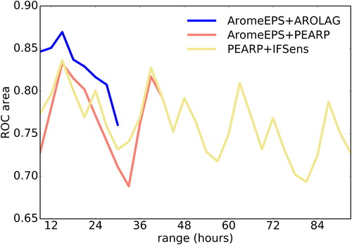
The lower left panel of Fig. 9 (i.e. ROC area for the PEARP + IFSens blend) shows a decreasing trend of the score as a function of range. Using the commonly quoted value of ROCA = 0.6 as a limit below which a forecast is no longer regarded as usable in practice, a visual linear fit to the ROC area curves suggests that the average thunderstorm predictability horizon is about 5 to 6 days over Western Europe, an estimate that is consistent with the work of Simon et al. (2018).

We have shown that multi-ensemble blends usually outperform single ensembles, but not always. At specific ranges, and for some classes of users (e.g. with specific cost-loss ratios), single ensembles can be better. The situation can arise when mixing two ensembles with very different forecast performance (such as AromeEPS and PEARP): the worse one can degrade some aspects of the blend, despite the tuning of parameter w that is supposed to weight the ensembles according to their relative performance. In this case, using multi-ensembles cannot justified by our scores, but it may be desirable for other reasons, such as the resilience of the forecasting system against a missing contributing ensemble, or the forecast continuity across a wide set of ranges.

Figure 10 shows the ROC area scores of the three multi-ensemble blends, compared over all considered forecast ranges. It demonstrates the complementarity between the high-resolution Arome-based blends that provide the best forecasts at short ranges, and the global PEARP and IFSens systems that cover longer ranges. The Arome-EPS + PEARP blend fails to provide forecasts of intermediate quality, probably because the Arome and Arpège models used are too different to be blended using our simple technique: Fig. 8a showed that PEARP had the smallest optimal radius r of all systems. The spatial neighbourhood operator has been found to be the most important component of the ensemble post-processing, and it may not be possible to find a single radius that performs well for both AromeEPS and PEARP. To correct this issue, one could perhaps use a better PEARP thunderstorm diagnostic (e.g. along the lines of the Lopez (2016)), or directly blend AromeEPS with IFSens.

The reliability of the multi-ensemble blends has been checked as follows, after out-of-sample calibration: over the three-month period, the average fraction of points with observed thunderstorms was 2.2%, and the average forecast probability of thunderstorm occurrence was 3.1% in AromeEPS + AROLAG, 2.6% in AromeEPS + PEARP, and 2.9% PEARP + IFSens at forecast ranges between 9 and 30 hours. These numbers mean that the calibration works well on the optimized blends, because the output probabilities are quite reliable.

7. Summary, discussion and conclusions

We have presented a new ensemble post-processing technique that combines different aspects of probabilistic forecasting: spatial tolerance using a neighbourhood operator, smoothing of the forecast density functions using a dressing operator, weighting between several ensembles, and adjustment of the threshold that diagnoses a binary event of interest (thunderstorm occurrence) from the NWP (numerical weather prediction) model output. These operators are controlled using only four tuning parameters that can be optimized on a rather short (about 1 month) training period, which makes the approach suitable for real-time application in operational meteorological institutes. The optimization is done by maximizing the ROC area, which is a measure of the end user value of probabilistic forecasts in terms of false alarm and detection rates. The optimization technique uses Latin hypercube sampling and a surrogate model algorithm, with a diagnostic of tolerance intervals around the estimated optimum parameter values. Output probabilities can be calibrated using an a posteriori rescaling, although more elaborate calibrations could be used.

The post-processing technique has been tested on thunderstorm forecasts. Only thunderstorm occurrence is predicted, not its intensity. The corresponding pseudo-observations have been generated from lightning and radar measurements. Three multi-ensemble systems, called ‘blends’, have been post-processed during 92 days of summer 2018, over mainland France. The dataset includes a wide variety of forecast ranges (from 9 to 93 h) and model resolutions (from 1.3 to 25 km horizontal mesh), using four operational ensembles: a poor man’s ensemble of lagged deterministic forecasts, a high-resolution limited area ensemble (AromeEPS), and two global ensembles (PEARP and IFSens).

The optimization of the post-processing parameters, as well as the calibration, appear to have enough statistical robustness for real-time operational applications. The robustness comes at the expense of neglecting variations between models, ensemble systems, and forecast times. Our diagnostics have shown that these variations may have significant implications. The optimized, blended superensembles have reasonable thunderstorm forecasting abilities, although they could probably be improved by including more tuning parameters to better account for the neglected parameter variability. These modifications to the post-processing system would require more computational resources and larger training datasets.

We recommend to further improve the proposed algorithm by making the (u, w, d) parameters dependent on the model type used (e.g. Arome, Arpège or IFS models), and by including some dependency with respect to diurnal time, which seems to be important. It would also be interesting for the tunings to depend on forecast range and on geographical location (preliminary testing has shown that our algorithm leads to different tunings if it is restricted to the Mediterranean area). The neighbourhood operator was limited to the space dimension in this study: it should be complemented by some time tolerance, in particular for models with an imperfect diurnal cycle of summer convection. Other model predictors of thunderstorm occurrence should be tested, in particular the PEARP CAPE diagnostic used here could be improved, because CAPE is only loosely related to the actual triggering of thunderstorms in numerical models.

Over regions and periods with less thunderstorm activity than in this paper, the automatic parameter tuning would be more difficult, because a minimum number of thunderstorm events is needed to achieve statistical stability: in an operational setting, the learning algorithm would need to be carefully warmed up at the beginning of each convective season, in particular if the NWP systems used have changed since the previous season. In production settings where reforecasts are not available, one could adjust the size of the learning dataset so that it always contains enough observed and forecast thunderstorm events to achieve statistical robustness. In some parts of the globe, the availability of ground-based lightning and radar data may be problematic, in which case thunderstorm products derived from satellite observations should be useful alternatives.

We have shown that the statistical post-processing has a large impact on the performance of the post-processed multi-ensembles. Probabilistic forecasts based on direct ensemble output (without any post-processing) usually benefit from higher model resolution and larger ensemble size, but as we have seen, this is not always true after post-processing: in some conditions, a poor man’s ensemble or a low-resolution global model can outperform more expensive NWP systems. The probabilistic forecast quality and the benefit of multi-ensembles also depends on the user cost-loss ratio – that is, on the relative cost that is attached to false alarms and to missed events. In a nutshell, multi-ensembles do not necessarily beat single-ensemble systems in all respects, but with a suitable post-processing they can be an attractive way of combining output from multiple systems, for specific user needs, and on a broad range of forecast horizons.

It would be useful to extend the approach used here to forecast violent thunderstorms. This would require a complexification of the observation definition (taking into account important meteorological variables such as gusts, hail and rain accumulation) and of the model diagnostics used. The rarity, and often low predictability, of these events will require larger training datasets, possibly including nowcasting products in the blending. This will be the topic of future work.

Acknowledgements

The lightning data was provided by the Météorage company. The manuscript was improved by the helpful comments of two anonymous reviewers.

Disclosure statement

No potential conflict of interest was reported by the authors.

Additional information

Funding

This work was funded by the French government through Météo-France and CNRS UMR3589.

Appendix:

Technical description of the parameter optimization

The optimization is performed in the four-dimensional space of input parameters (r, d, w, u), except when a single ensemble is being used, in which case the space reduces to (r, d, u). The objective function is the ROCA score (i.e. the area under the ROC curve), averaged over each considered month and forecast ranges: for each vector of input parameters, the thunderstorm probabilities are computed over the training period, and the ROCA score is derived from this verification against lightning/radar observations.

The input parameter space is sampled using a Latin hypercube centred maximin strategy (Deutsch and Deutsch, 2012), implemented in Python language by the pyDOE package (documentation and code available at https://pythonhosted.org/pyDOE/index.html). We used a sample of size 100, beyond which little improvement was found. The user-specified search interval of each parameter is transformed using an exponential mapping, so that smaller parameter values are more densely sampled than larger ones.

The ROCA value is then computed at each sample point. This is the most computationally expensive part: training over one calendar month takes from 6 to 30 h of single-core computing on a modern desktop PC, depending on the ensemble size. With some parallelization, this time could easily be divided by a factor 1000.

Next, the ROCA points are interpolated by a smooth four-dimensional function, called surrogate function, using a Gaussian regression process algorithm. The scikit-learn machine learning package was used (https://scikit-learn.org/0.17/modules/gaussian_process.html). The surrogate function approximates the dependency of ROCA on the input parameters, and it is much cheaper to evaluate.

Finally, a numerical optimizer (BFGS, from the Python scipy library) is used to locate the maximum of the surrogate function. The optimization is restarted from each of the 100 ROCA sample points in order to increase the likelihood that the absolute maximum will be reached. In all tested configurations, the ROCA optimum was found to be significantly better than all sample points, and it belonged to the interior of the search domain. In other words, the result was not sensitive to the chosen parameter boundaries.

Fig. 1. Left panel: Lightning flashes from the Météorage network (9 August 2018, 00UTC), the colours indicate the number of strokes per flash. Right panel: Pseudo-observations of thunderstorms (light bullets: non-occurrence, dark bullets: occurrence).

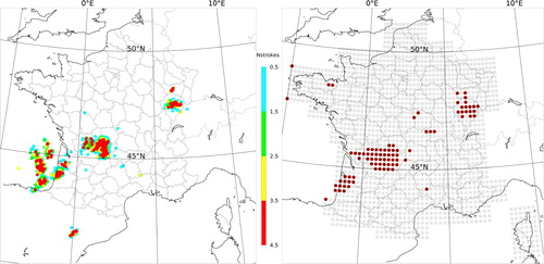
Fig. 2. Timings of the four ensembles considered in the paper, relative to the same 00UTC production base. The thick horizontal arrows indicate the forecasts runs (deterministic and ensembles); the dashed horizontal segments indicate forecast ranges that are computed but not used (some forecasts may also extend further into the future than represented here). Grey boxes and arrows indicate the ensembles and tuning windows used in each ensemble blend. The model grid resolution is given next to each ensemble name.

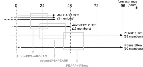
Fig. 3. ROC diagrams of the AromeEPS ensemble thunderstorm forecasts, without any post-processing (‘raw ensemble’), with the 20 km neighbourhood operator (‘neigh’), with neighbourhood and dressing operators (‘neigh + dress’, with d = 1), and with the neighbourhood operator with a re-tuned threshold u (‘neigh + thres’, made with u = 8, instead of 10 in the other curves). The diagrams are computed over June, July and August 2018 (i.e. 92 days), on forecast ranges from 12 to 42 h. The apparent differences between the ROC areas are significant at the 95% level. The respective ROC areas are 0.54, 0.72, 0.77, 0.74, and the ROC area with the combined neighbourhood, dressing operators and retuned threshold (curve not shown) is 0.78.

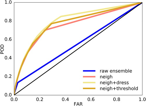
Fig. 4. 1D transects of the ROCA(r, d, w, u) surrogate function around the optimum, for the AromeEPS + AROLAG ensemble mix, over June 2018. The curves have been horizontally rescaled so that the optimum is at zero, values below (resp. above) the optimum have been linearly rescaled from their minimum (resp. maximum) search value to −1 (resp. +1).

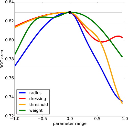
Fig. 5. Optimized values of the parameters (r, d, w, u) i.e. (radius, dressing, weight, threshold) for three ensemble blends, over 3 independent periods (June, July and August 2018). The blue bars show the values that optimize the ROCA area, the black vertical bars show the uncertainty interval that is implied by the optimization procedure.

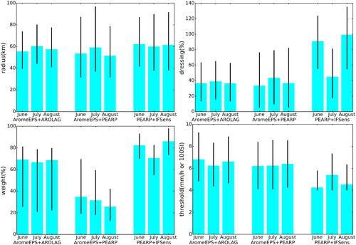
Fig. 6. Reliability diagrams for the AromeEPS + AROLAG blend where (r, d, w, u) have been optimized over June 2018. The curves are displayed before and after applying the reliability calibration procedure. The numbers indicate the sample size used to compute each point (K means 1000).

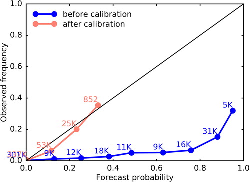
Fig. 7. Thunderstorm probability forecasts based on 8 August 2018, 00UTC and valid 24 h later, forecast by (from left to right) the raw Arome-EPS ensemble, the calibrated AromeEPS + AROLAG, AromeEPS + PEARP and PEARP + IFSens blends. The black disk indicates the city of Bordeaux.

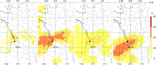
Fig. 8. Values of tuning parameters (r, d, u) i.e. (radius, dressing, threshold), independently optimized for each ensemble used in the blends. The optimization is done over June 2018. The graphical conventions are as in Fig. 5.

Fig. 9. ROC areas and potential economic values of the forecast thunderstorm probabilities, for the three ensemble blends (one per row) and their contributing ensembles. The plots are averaged over 92 days. The potential economic value diagrams (right column) are averaged over the same forecast ranges as the ROC areas (left). Bullets are plotted on the ROCA curves when the contributor score is statistically significant from the blend score.

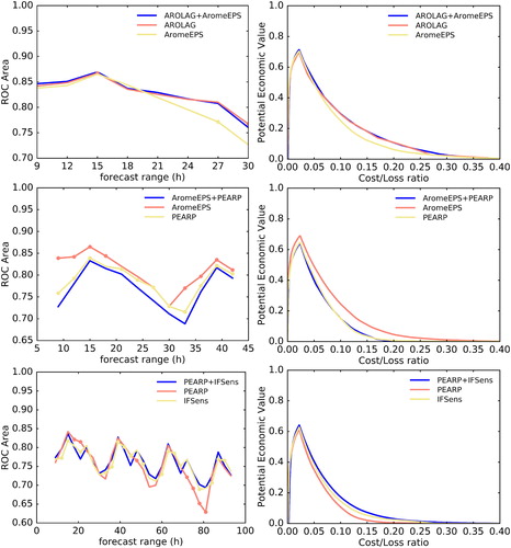
Fig. 10. ROC areas of the three blends, over their respective forecast ranges, averaged over 92 days.

References

- Beck, J., Bouttier, F., Wiegand, L., Gebhardt, C., Eagle, C. and co-authors. 2016. Development and verification of two convection-resolving multi-model ensembles over northwestern Europe. Q. J. R. Meteorol. Soc. 142, 2808–2826, doi:10.1002/qj.2870
- Ben Bouallègue, Z. 2013. Calibrated short-range ensemble precipitation forecasts using extended logistic regression with interaction terms. Weather Forecast. 28, 515–524, doi:10.1175/WAF-D-12-00062.1
- Berrocal, V. J., Raftery, A. E. and Gneiting, T. 2007. Combining spatial statistical and ensemble information in probabilistic weather forecasts. Mon. Weather Rev. 135, 1386–1402, doi:10.1175/MWR3341.1
- Bouttier, F., Vié, B., Nuissier, O. and Raynaud, L. 2012. Impact of stochastic physics in a convection-permitting ensemble. Mon. Weather Rev. 140, 3706–3721, doi:10.1175/MWR-D-12-00031.1
- Bouttier, F., Raynaud, L., Nuissier, O. and Ménétrier, B. 2016. Sensitivity of the AROME ensemble to initial and surface perturbations during HyMeX. Q. J. R. Meteorol. Soc. 142, 390–403, doi:10.1002/qj.2622
- Bröcker, J. and Smith, L. 2008. From ensemble forecasts to predictive distribution functions. Tellus A: Dyn. Meteorol. Oceanogr. 60, 663–678, doi:10.1111/j.1600-0870.2008.00333.x
- Brousseau, P., Seity, Y., Ricard, D. and Léger, J. 2016. Improvement of the forecast of convective activity from the AROME-France system. Q. J. R. Meteorol. Soc. 142, 2231–2243, doi:10.1002/qj.2822
- Casati, B. and Wilson, L. J. 2007. A new spatial-scale decomposition of the Brier score: application to the verification of lightning probability forecasts. Mon. Weather Rev. 135, 3052–3069, doi:10.1175/MWR3442.1
- Clark, A. J., Gallus, W. A. and Chen, T. C. 2008. Contributions of mixed physics versus perturbed initial/lateral boundary conditions to ensemble-based precipitation forecast skill. Mon. Weather Rev. 136, 2140–2156, doi:10.1175/2007MWR2029.1
- Clark, A. J., Gallus, W. A., Xue, M. and Kong, F. 2009. A comparison of precipitation forecast skill between small convection-allowing and large convection-parameterizing ensembles. Weather Forecast. 24, 1121–1140, doi:10.1175/2009WAF2222222.1
- Collins, W. and Tissot, P. 2015. An artificial neural network model to predict thunderstorms within 400 km2 South Texas domains. Meteorol. Appl. 22, 650–665, doi:10.1002/met.1499
- Descamps, L. and Talagrand, O. 2007. On some aspects of the definition of initial conditions for ensemble prediction. Mon. Weather Rev. 135, 3260–3272, doi:10.1175/MWR3452.1
- Descamps, L., Labadie, C., Joly, A., Bazile, E., Arbogast, P. and co-authors. 2015. PEARP, the Météo-France short-range ensemble prediction system. Q. J. R. Meteorol. Soc. 141, 1671–1685, doi:10.1002/qj.2469
- Deutsch, J. L. and Deutsch, C. V. 2012. Latin hypercube sampling with multidimensional uniformity. J. Stat. Plan. Inference 142, 763–772, (with online material at https://github.com/sahilm89/lhsmdu). doi:10.1016/j.jspi.2011.09.016
- Flowerdew, J. 2014. Calibrating ensemble reliability whilst preserving spatial structure. Tellus A: Dyn. Meteorol. Oceanogr. 66, 22662, doi:10.3402/tellusa.v66.22662
- Gijben, M., Dyson, L. L. and Mattheus, T. L. 2017. A statistical scheme to forecast the daily lightning threat over Southern Africa using the Unified Model. Atmos. Res. 194, 78–88, doi:10.1016/j.atmosres.2017.04.022
- Gneiting, T., Raftery, A. E., Westveld, A. H. and Goldman, T. 2005. Calibrated probabilistic forecasting using ensemble model output statistics and minimum CRPS estimation. Mon. Weather Rev. 133, 1098–1118, doi:10.1175/MWR2904.1
- Goodman, S. J., Blakeslee, R. J., Koshak, W. J., Mach, D., Bailey, J. and coauthors. 2013. The GOES-R geostationary lightning mapper (GLM). Atmos. Res. 125, 34–49,
- Hagedorn, R., Buizza, R., Hamill, T. M., Leutbecher, M. and Palmer, T. N. 2012. Comparing TIGGE multimodel forecasts with reforecast-calibrated ECMWF ensemble forecasts. Q. J. R. Meteorol. Soc. 138, 1814–1827, doi:10.1002/qj.1895
- Hamill, T. M., Whitaker, J. S. and Mullen, S. L. 2006. Reforecasts: an important dataset for improving weather predictions. Bull. Am. Meteorol. Soc. 87, 33–46, doi:10.1175/BAMS-87-1-33
- Hamill, T., Hagedorn, R. and Whitaker, J. S. 2008. Probabilistic forecast calibration using ECMWF and GFS ensemble reforecasts. Part II: Precipitation. Mon. Weather Rev. 136, 2620–2632, doi:10.1175/2007MWR2411.1
- Jolliffe, I. T. and Stephenson, D. B. 2011. Forecast Verification: A Practitioner's Guide in Atmospheric Science. 2nd ed. John Wiley and Sons, Hoboken, NJ, 292 pp,
- Karagiannidis, A., Lagouvardos, K., Lykoudis, S., Kotroni, V., Giannaros, T. and co-authors. 2019. Modeling lightning density using cloud top parameters. Atmos. Res. 222, 163–171, doi:10.1016/j.atmosres.2019.02.013
- Keil, C., Heinlein, F. and Craig, G. C. 2014. The convective adjustment time-scale as indicator of predictability of convective precipitation. Q. J. R. Meteorol. Soc. 140, 480–490, doi:10.1002/qj.2143
- Leutbecher, M., Lock, S.-J., Ollinaho, P., Lang, S. T. K., Balsamo, G. and co-authors. 2017. Stochastic representations of model uncertainties at ECMWF: state of the art and future vision. Q. J. R. Meteorol. Soc. 143, 2315–2339, doi:10.1002/qj.3094
- Leutbecher, M. 2018. Ensemble size: how suboptimal is less than infinity? Q. J. R. Meteorol. Soc. 145, 1–22,
- Li, N., Wei, M., Niu, B. and Mu, X. 2012. A new radar-based storm identification and warning technique. Meteorol. Appl. 19, 17–25, doi:10.1002/met.249
- Lopez, P. 2016. A lightning parameterization for the ECMWF integrated forecasting system. Mon. Weather Rev. 144, 3057–3075, doi:10.1175/MWR-D-16-0026.1
- Lu, C., Yuan, H., Schwartz, B. E. and Benjamin, S. G. 2007. Short-range numerical weather prediction using time-lagged ensembles. Weather Forecast. 22, 580–595, doi:10.1175/WAF999.1
- Mason, S. and Graham, N. 1999. Conditional probabilities, relative operating characteristics, and relative operating levels. Weather Forecast. 14, 713–725, > 2.0.CO;2. doi:10.1175/1520-0434(1999)014<0713:CPROCA>2.0.CO;2
- Osinski, R. and Bouttier, F. 2018. Short-range probabilistic forecasting of convective risks for aviation based on a lagged-average-forecast ensemble approach. Meteorol. Appl. 25, 105–118, doi:10.1002/met.1674
- Park, Y.-Y., Buizza, R. and Leutbecher, M. 2008. TIGGE: Preliminary results on comparing and combining ensembles. Q. J. R. Meteorol. Soc. 134, 2029–2050, doi:10.1002/qj.334
- Pédeboy, S. and Schulz, W. 2014. Validation of a ground strike point identification algorithm based on ground truth data. In: Abstracts of the 23rd International Lightning Detection Conference, Tucson, AZ, 7 pp. Online at: https://www.meteorage.com/
- Raftery, A., Gneiting, T., Balabdaoui, F. and Polakowski, M. 2005. Using Bayesian model averaging to calibrate forecast ensembles. Mon. Weather Rev., 133, 1155–1174, doi:10.1175/MWR2906.1
- Raynaud, L. and Bouttier, F. 2016. Comparison of initial perturbation methods for ensemble prediction at convective scale. Q. J. R. Meteorol. Soc. 142, 854–866, doi:10.1002/qj.2686
- Richardson, D. 2000. Skill and relative economic value of the ECMWF ensemble prediction system. Q. J. R. Meteorol. Soc. 126, 649–667, doi:10.1002/qj.49712656313
- Scheuerer, M. 2014. Probabilistic quantitative precipitation forecasting using ensemble model output statistics. Q. J. R. Meteorol. Soc. 140, 1086–1096, doi:10.1002/qj.2183
- Schmeits, M. J., Kok, K. J., Vogelezang, D. H. P. and van Westrhenen, R. M. 2008. Probabilistic forecasts of (severe) thunderstorms for the purpose of issuing a weather alarm in the Netherlands. Weather Forecast. 23, 1253–1267, doi:10.1175/2008WAF2007102.1
- Schwartz, C. S. and Sobash, R. A. 2017. Generating probabilistic forecasts from convection-allowing ensembles using neighborhood approaches: a review and recommendations. Mon. Weather Rev. 145, 3397–3418, doi:10.1175/MWR-D-16-0400.1
- Seity, Y., Brousseau, P., Malardel, S., Hello, G., Bénard, P. and co-authors. 2011. The AROME-France convective scale operational model. Mon. Weather Rev. 139, 976–991, doi:10.1175/2010MWR3425.1
- Simon, T., Fabsic, P., Mayr, G. J., Umlauf, N. and Zeileis, A. 2018. Probabilistic forecasting of thunderstorms in the Eastern Alps. Mon. Weather Rev. 146, 2999–3009, doi:10.1175/MWR-D-17-0366.1
- Sobash, R. A., Kain, J. S., Bright, D. R., Dean, A. R., Coniglio, M. C. and co-authors. 2011. Probabilistic forecast guidance for severe thunderstorms based on the identification of extreme phenomena in convection-allowing model forecasts. Weather Forecast. 26, 714–728, doi:10.1175/WAF-D-10-05046.1
- Taillardat, M., Mestre, O., Zamo, M. and Naveau, P. 2016. Calibrated ensemble forecasts using quantile regression forests and ensemble model output statistics. Mon. Weather Rev. 144, 2375–2393, doi:10.1175/MWR-D-15-0260.1
- Theis, S. E., Hense, A. and Damrath, U. 2005. Probabilistic precipitation forecasts from a deterministic model: a pragmatic approach. Meteorol. Appl. 12, 257–268, doi:10.1017/S1350482705001763
- Walser, A., Lüthi, D. and Schär, C. 2004. Predictability of precipitation in a cloud-resolving model. Mon. Weather Rev. 132, 560–577, > 2.0.CO:2. doi:10.1175/1520-0493(2004)132<0560:POPIAC>2.0.CO;2
- Weisman, M. L., Davis, C., Wang, W., Manning, K. W. and Klemp, J. B. 2008. Experiences with 0–36 h explicit convective forecasts with the WRF-ARW Model. Weather Forecast. 23, 407–437, doi:10.1175/2007WAF2007005.1
- Yair, Y., Lynn, B., Price, C., Kotroni, V., Lagouvardos, K. and co-authors. 2010. Predicting the potential for lightning activity in Mediterranean storms based on the weather research and forecasting (WRF) model dynamic and microphysical fields. J. Geophys. Res. 115, D04205,
- Zhu, Y., Toth, Z., Wobus, R., Richardson, D. and Mylne, K. 2002. The economic value of ensemble-based weather forecasts. Bull. Am. Meteorol. Soc. 83, 73–83, doi:10.1175/1520-0477(2002)083<0073:TEVOEB>2.3.CO;2
- Ziehmann, C. 2000. Comparison of a single-model EPS with a multi-model ensemble consisting of a few operational models. Tellus A: Dyn. Meteorol. Oceanogr. 52, 280–299, doi:10.3402/tellusa.v52i3.12266