Using land-based stations for air–sea interaction studies

Abstract

In situ measurements representing the marine atmosphere and air–sea interaction are taken at ships, buoys, stationary moorings and land-based towers, where each observation platform has structural restrictions. Air–sea fluxes are often small, and due to the limitations of the sensors, several corrections are applied. Land-based towers are convenient for long-term observations, but one critical aspect is the representativeness of marine conditions. Hence, a careful analysis of the sites and the data is necessary. Based on the concept of flux footprint, we suggest defining flux data from land-based marine micrometeorological sites in categories depending on the type of land influence:

• 1. CAT1: Marine data representing open sea,

• 2. CAT2: Disturbed wave field resulting in physical properties different from open sea conditions and heterogeneity of water properties in the footprint region, and

• 3. CAT3: Mixed land–sea footprint, very heterogeneous conditions and possible active carbon production/consumption.

Characterization of data would be beneficial for combined analyses using several sites in coastal and marginal seas and evaluation/comparison of properties and dynamics. Aerosol fluxes are a useful contribution to characterizing a marine micrometeorological field station; for most conditions, they change sign between land and sea sectors. Measured fluxes from the land-based marine station Östergarnsholm are used as an example of a land-based marine site to evaluate the categories and to present an example of differences between open sea and coastal conditions. At the Östergarnsholm site the surface drag is larger for CAT2 and CAT3 than for CAT1 when wind speed is below 10 m/s. The heat and humidity fluxes show a distinctive distinguished seasonal cycle; latent heat flux is larger for CAT2 and CAT3 compared to CAT1. The flux of carbon dioxide is large from the coastal and land–sea sectors, showing a large seasonal cycle and significant variability (compared to the open sea sector). Aerosol fluxes are partly dominated by sea spray emissions comparable to those observed at other open sea conditions.

Keywords:

• air–sea interaction
• coastal zone
• carbon dioxide
• micrometeorological measurements
• sea spray

1. Introduction

The surface of the Earth is dominated by oceans. Covering ca 70% of the area, oceans as well as air–sea interaction are important components in any global modelling system. About 7% of the world ocean area can be defined as coastal regions (Gattuso et al., 1998). Marginal seas and coastal areas are key areas in the global carbon cycle, as they support a significant portion of the global primary productivity and draw a substantial flux of atmospheric CO₂ into the ocean (Chen et al., 2013). Muller-Karger et al. (2005) estimated that the shelf seas might be responsible for as much as 40% of the global oceanic carbon sequestration. In addition, marginal and mediterranean seas are active regions when considering recreation, renewable energy production, transport and marine food production.

Historically, there has been less focus on marine processes compared to terrestrial processes when understanding the atmosphere–surface interaction, as the ocean surface is generally considered more homogeneous; air–sea processes and interactions are also more difficult to measure and to continuously monitor. As the ocean surface responds differently compared to a land surface with a completely different response time scale for the mixing, and with a surface roughness changing as a response of the atmospheric forcing, it is important to understand and characterize air–sea interaction and air–sea fluxes over open sea as well as in coastal regions.

Micrometeorological in situ measurements representing the marine atmosphere can be made at ships, drifting buoys, stationary moorings, or aircraft, or at land-based towers. These different settings are complementary and have different advantages and disadvantages. CO₂ fluxes over the sea are often small, and several corrections usually need to be applied due to the limitations of the presently available sensors and sampling systems. On seaborne platforms these measurements generally represent open sea conditions and offer a way to monitor a larger area, but they are demanding to conduct, as the movements of the platform and the flow distortion caused by the structures of the platform itself influence the measurements, and these movements need to be handled in a proper way. The movements of a seaborne platform can be minimized, as in the case of specially designed platforms like FLIP (Anderson et al., 2004), but generally the motion of the platform has to be measured and corrected for (e.g. Anctil et al., 1994; Pedreros et al., 2003; Miller et al., 2010; Landwehr et al., 2015). The seaborne platforms are usually used only for limited periods from a few weeks to a few months. Aircraft are typically used to fly one or several legs in different levels or at different altitudes per day, each of them lasting only a few hours. Ships and aircraft are comparably expensive to operate.

To obtain continuous, long-term air–sea interaction measurements, fixed installations are needed. The ideal installation would be a tower placed in water deep enough to represent open sea conditions. Few such platforms are, or have been in use (BIO, Smith, 1980; Noordwijk, DeCosmo et al., 1996; FINO1, Neumann and Nolopp, 2007). By using fixed towers, motion corrections are avoided, and it is also possible to design the site and the set-up so that flow distortion is very limited. For practical reasons, land-based towers are easier to construct, access and run. One needs, however, to be very careful to make sure the measurements represent the sea area one wishes to study, and it is crucial to make a careful analysis of the site and the data before using land-based towers to study air–sea interaction. With the technological development and the increased potential of micrometeorological stations for land-based studies, and the increasing need for long-term measurements, there is a growing interest for setting up coastal stations for air–sea interactions studies. Marine stations for monitoring meteorological and air-quality properties have been active for many years (e.g. Mace Head, O’Connor et al., 2008), but marine sites using micrometeorological methods are less common. For a site to be suitable for micrometeorological measurements, several requirements of the site and instrumentation are different compared to sites monitoring average properties of the atmosphere. There is an ongoing expansion of land-based marine stations that also include micrometeorological instrumentation, such as the Penelee Point Observatory (Yang et al., 2016), the Utö station (http://en.ilmatieteenlaitos.fi/uto, Engler et al., 2007) and the Östergarnsholm marine micrometeorological station (e.g. Smedman et al., 1999; Rutgersson et al., 2008).

For any station situated in a coastal zone or marginal sea, some influence of the nearby land areas is unavoidable. Here, we aim at defining criteria to be used when characterizing a land-based marine site and its data. Defining different data categories will make comparisons with open sea data more relevant and also make it possible to relate results from different sites and coastal regions to each other. The flux footprint is a central concept for micrometeorological measurements. It is defined as the upwind region influencing the measurements, and it depends on the stability, surface roughness, wind direction and measurement height. For in situ measurements, the flux footprint area is situated in the order of a few hundred metres to several kilometres upwind of the sensors. As the data represent the conditions of the footprint area, the definitions of data categories are based on wind direction and the water-side conditions of the respective footprint area.

We are using the well investigated Östergarnsholm station as an example of how to evaluate a site. We also present examples of results obtained using data from the Östergarnsholm site. A suggestion on relevant categories to be used to define flux data from land-based sites is presented in Section 2. The Östergarnsholm site is described in Section 3, and a suggested methodology on how to characterize a land-based site when using it for marine studies in Section 4. In Section 5 various properties for the different categories of Östergarnsholm are presented. The generality of the results is discussed in Section 6.

2. Category characterization

In this characterization we suggest defining the categories of data from two different aspects (1) physical, defining the site/data according to the representativeness of the turbulence properties, heat, momentum and aerosol fluxes, and (2) biogeochemical, defining the site/data based on the representativeness with respect to water-side chemistry.

The impact of the nearby land areas on the measurements varies in importance depending on the interpretation of the measurements and, of course, the research to be performed. One type of impact is from mesoscale circulation systems in the atmosphere or in the sea. Due to the land–sea contrast, mesoscale systems in the vicinity of a coast are generally stronger compared to mesoscale systems that may occur in the open ocean, as they are often generated by land–sea difference in time or space. Examples are processes generated by air–sea temperature contrasts, such as sea breeze circulations, low-level jets (LLJs, e.g. Källstrand et al., 2000) or horizontal rolls (Svensson et al., 2017). Coastal areas are influenced by riverine outflow resulting in respiration of terrestrial organic carbon inputs, benthic–pelagic coupling, variability in surfactant abundance and near-surface vertical stratification (Rutgersson et al., 2011). Coastal sea areas have seasonal horizontal gradients of temperature and salinity, as well as upwelling events (e.g. Sproson and Sahlée, 2014). The local currents are modified by the land masses close by. At higher latitudes the coastal areas often get a seasonal ice cover of variable extent. The horizontal scale of these circulation systems ranges from tens to several hundred kilometres, and the consequence of these systems on the measured data is a larger variability in time and space of a variety of parameters compared to data taken at open sea areas. One can thus consider land-based sites as large-scale laboratories to study various phenomena, as there is often a wider range available in terms of stratification and gradients. One implication is also often large air–sea differences, which give large vertical fluxes and thus large signal-to-noise ratios of micrometeorological measurements compared to open sea areas. These impacts are expected to be present at all stations in coastal and marginal seas and are not possible to avoid. As long as the mesoscale systems have a great enough scale (in time and space) not to invalidate assumptions of stationarity and homogeneity, this does not disturb the measurements or the assumption of representativeness for open sea conditions when studying air–sea interaction processes. If such mesoscale systems are the only land influence of a site, we suggest characterizing the station as category 1, in which the data and physical processes represent open sea turbulence, fluxes and air–sea interactions. For the category 1 characterization, surface properties are expected to be homogeneous, and thus one marine mooring to measure the wave field, surface water temperature or biogeochemical properties will well represent the flux footprint of the measurements taken at the land-based tower. It should here be noted that some mesoscale systems have a small spatial or temporal scale compared to the flux footprint area and induce great heterogeneity; one such example is upwelling conditions having great influence of the properties of the water as well as atmosphere (e.g. Norman et al., 2013; Sproson and Sahlée, 2014). Such situations should be filtered out for category 1 data.

The bottom topography surrounding a coastal station often changes the characteristics of the wave field due to shoaling, and its properties strongly depend on the wavelength. When waves enter in shallower water, they get steeper, and depending on the wavelength might break at different distances from the coast. Irregular topography can cause convergence or divergence of wave energy, and the direction of the waves can change. Coastlines that are steep enough can reflect the waves back towards the open sea or break, raising the water and spray several times higher than the original wave. As the wave field directly influences the physical aspects of air–sea interaction (turbulence properties, surface drag, wind gradient, and also heat and humidity flux), the data from cases with a transformed wave field do not represent open sea conditions, and data are categorized as category 2 for the physical properties. With a changing wave field, it is also very likely that the sea spray production as well as dry deposition of particles changes significantly (Schack et al., 1985). Both would change the aerosol fluxes, but there are limited in situ data confirming this. The direct or indirect impact of waves via different scales of turbulence on gas fluxes is not fully known (Garbe et al., 2014). It is likely that biogeochemical fluxes also are influenced by the changes in wave fields, and thus it is suggested that the biogeochemical categorization also be defined as category 2. If the measured fluxes are related to properties of the water surface, it is important to make sure that the footprint is represented by the water-side measurements (i.e. the moorings or water sampling sites need to represent the flux footprint of the measurements). This is not the case if the biogeochemical properties are very heterogeneous, situations that can be expected to be more frequent at a land-based site than in the open sea.

If the flux footprint area of the measurements is over the actual shore or shallow near-shore regions, the turbulence and fluxes are influenced by the land areas in a disproportional way (as the roughness of a land surface is significantly larger compared to the water surface); then, the data are categorized as category 3. For towers situated further inland from the shore, or within an archipelago, the flux footprint likely consists of a combination of land surface and shore-area water surfaces. These areas can be very active in a biogeochemical sense. Aerosol fluxes add additional information when estimating the land vs. ocean influence on the footprint. In the absence of primary aerosol sources, dry deposition dominates the aerosol fluxes, resulting in a negative (downward) net aerosol flux over land. See Buzorius et al. (2001) for boreal forests, Grönlund et al. (2002) for Antarctic snow fields or Ahlm et al. (2010) for the Amazonian rainforests. The same applies to sea ice; see Nilsson and Rannik (2001). Over ocean, on the other hand, sea spray formation dominates over deposition already from a wind speed of a few m/s (Nilsson et al., 2001; Geever et al., 2005), resulting in an upward (positive) aerosol flux.

The main categories for ice-free sea can be defined as

1. Open sea (CAT1): Marine station, a wave field undisturbed by topographical or coastal features, water-side measuring system representative of the flux footprint of the tower. Mesoscale circulation system in sea or atmosphere might influence the measurements.

2. Coastal sea (CAT2): A local wave field influenced by bathymetry or limited fetch resulting in physical properties different from open sea conditions or strong gradients of temperature and salinity in the footprint region due to the water depth. In a near surface region the biogeochemical properties can vary, even if the physical ones do not. This can originate from differences in the biogeochemical input via runoff from land or variation in biological activity in the vicinity of land and more shallow water.

3. Mixed land–sea area (CAT3): Mixed land–sea footprint of the tower with very heterogeneous physical and biogeochemical conditions, where, with only few water-side measurements, it is not possible to fully represent water-side conditions.

Data from one station usually represent different categories depending on the wind direction, measurement height, other environmental constraints and the parameter of interest. Hence, the characterization should be done for specific wind-direction intervals, depending on the properties of the site. Data in category 3 can include a parameter describing the land–sea fraction. Measurements over sea ice form a category of their own in addition to these three discussed in this paper. It would also be possible to divide category 2 into subcategories (including factors like impact of limited water depth, limited fetch, disturbances of islands).

3. Östergarnsholm

3.1. Station, meteorology and gases

The station used to define characteristic properties for coastal/marginal sea stations is the marine ICOS (Integrated Carbon Observatory System) station Östergarnsholm situated in the Baltic Sea, 57°25′48.4″N 18°59′02.9″E (see Fig. 1). The main tower is a land-based, 30 m high tower situated on the southern tip of a very small, flat island (Fig. 2). Measurements at the site have been taken semi-continuously since 1995, and data have been used in numerous air–sea interaction studies (e.g. Smedman et al., 1999; Rutgersson et al., 2001; Högström et al., 2008; Sahlée et al., 2008b). The tower is equipped with high-frequency instrumentation for the turbulence measurements and slow-response sensors for mean profile measurements. The wind speed, wind direction, and temperature are measured at five levels, namely, 7, 11.5, 14, 20 and 28 m above the tower base. For the present system, high-frequency wind components are measured with CSAT3-3D sonic anemometers (Campbell Sci, Logan, UT, USA) at two levels, namely, 9 and 25 m above the tower base. The humidity and CO₂ fluctuations are measured with two LI-7500 open-path analysers at 9 and 25 m, and temporarily with a LI-7200 enclosed path analyser (LI-COR Inc., Lincoln, NE, USA). There are also additional measuring systems (including measurements of relative humidity, air pressure, global radiation, precipitation and vertical profiles of CO₂ and H₂O). Tides in the Baltic Sea are very small, and at the location of the site the sea level variations are moderate: the tower base is generally 1 ± 0.5 m above mean sea level.

Fig. 1. The Baltic Sea and the Östergarnsholm field station. The positions of the tower, the SAMI sensor and a Directional Waverider buoy (DWR) are shown by arrows in the lower figure. Thin lines in the lower figure represent isolines of water depth. Figure redrawn from Rutgersson and Smedman (2010). Blue lines illustrate the different wind direction sectors.

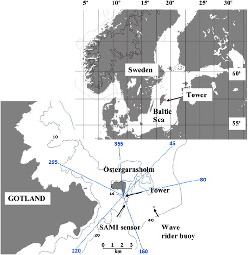
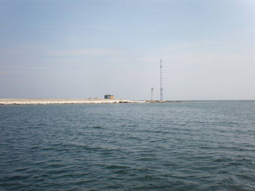
Fig. 2. The two towers at the Östergarnsholm station (facing east). The 30 m high tower is for flux and meteorological measurements, and the 10 m high tower for aerosol measurements.

3.2. Station, aerosols

In the summer of 2011 a 10 m high tower for aerosol flux measurements was added to the station by Stockholm University. The instrumentation includes an asymmetric ultrasonic anemometer Gill HS50, an open-path infrared CO₂ and H₂O analyser (Licor 7500, LI-COR, Inc., Lincoln, NE, USA), an optical particle counter (OPC) (Model1.109, Grimm Ainring, Bayern, Germany) and a condensation particle counter (CPC) TSI 3762 (TSI Inc., Shoreview, MN, USA). The sonic and the Licor are located at 12 m height. From the same height we sample the aerosol through ¼ inch stainless steel tubes to the CPC and OPC. The CPC counts the aerosol number for particles >10 nm particle diameter (D_p). The OPC counts and sizes the particles in 15 size bins from 0.25 to 2.5 µm D_p. For the OPC the number size distribution is also integrated to form particulate matter (PM) <1 µm D_p and 2.5 µm D_p, in literature and air quality legislation referred to as PM1 and PM2.5.

3.3. Station, sea

At a mooring located 1 km SE of the tower continuous measurements of water chemistry are conducted. For CO₂, a submersible autonomous moored instrument, so-called SAMI sensor (Sunburst Sensors, Missoula, MO, USA) is used. For dissolved oxygen and electrical conductivity, we use an SBE 37 Microcat IDO sensor (Seabird Electronics Inc., Bellevue, WA, USA). In addition, an EXO2 multi-parameter sensor (YSI Inc., Yellow Springs, OH, USA) is measuring pH, chlorophyll a, turbidity, electrical conductivity and fluorescent dissolved organic matter (fDOM). All sensors measure water temperature and are collectively mounted in a cage at a depth of approximately 5 m. The CO₂ and dissolved oxygen sensors measure at a 30/60 min temporal resolution, whereas the measuring resolution for the EXO2 sensor is bi-hourly. In close connection to the sensor cage a profile system is deployed measuring electrical conductivity and water temperature (Hobo U24) at the water-depths of 0.5, 1, 4, 8 and 20 m (Onset, Bourne, MA, USA) (see Fig. 1). The water depth at the mooring site is approximately 22 m. In addition to the sensor measurements, a manual water chemistry sampling programme has been running since 2015, with monthly water samples from April to November taken at three depths (0.5, 10 and 18 m) in accordance with the mooring described above. The samples are analysed in the lab according to accredited methods for pH, total phosphorus (TP), phosphate (PO₄), total nitrogen (TN), nitrate (NO₃), ammonium (NH₄) and dissolved silica (DSi).

Measurements of waves and their directional properties are made with a Directional Waverider moored 4 km southeast of the tower, where the water depth is 39 m. The buoy is run by the Finnish Meteorological Institute (FMI) and also measures water temperature at a depth of 0.5 m.

3.4. Specific campaigns 2012 and 2014

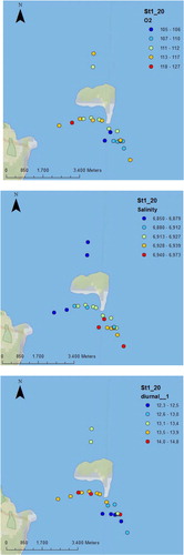
The spatial variations of the water properties were studied during three one-day cruises in June 2012, with measurements taken at 20 different stations (see Fig. 3). At some stations the measurements were done at multiple occurrences, giving in total 23 surface-water data points. Measurements of salinity, O₂ and temperature were taken using the SBE 37-SMP-IDO MicroCAT sensor; the instrument ran at least 20 min at the same point for an accurate measure.

Fig. 3. The horizontal water variation of diurnal corrected data of (upper) O₂ saturation in %, (middle) salinity in PSU and (lower) temperature in °C, data taken in June 2012.

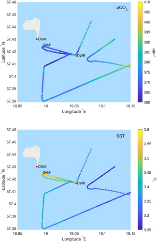
The Finnish research vessel Aranda visited the sea area outside Östergarnsholm during an FMI research cruise in April 2014 and monitored the sea surface pCO₂, salinity and sea surface temperature in the area (Fig. 4). The pCO₂ at four metres below the surface was measured with Kongsberg Contros HydroC via ship’s flow-through system. The sensor was submerged in seawater in an insulated tank of 100 litres in the laboratory. The water flowed past the sensor membrane and an external thermometer and discharged to the tank: the water in the tank turned over at a rate of 10 litres/minute. The measurements were corrected for the baseline drift and span by the manufacturer, and finally the corrections to in situ temperatures were made according to Takahashi et al. (1993). Sea surface temperature and salinity measurements at the depth of four metres, as well as basic meteorological and navigational information, were included in the routine observations on board.

Fig. 4. pCO₂ (upper) and temperature (lower) at 4 m depth from R/V Aranda's cruise 8 and 10 April 2014. Östergarnsholm tower is denoted by OGM, the moored pCO₂ sensor by SAMI and the Directional Waverider by DWR.

4. Methodology

A variety of aspects of a site should be evaluated when examining the quality of the site and the characterization of the data. The properties of the site need to be characterized, and quality control of the data is required. We here apply these steps to the Östergarnsholm site as an example of a land-based marine micrometeorological station, using the measurements at a height of 10 m above the sea surface from the main mast (12 m for aerosols) from the sea surface.

4.1. Characterizing a site

There are a number of factors to consider when examining a micrometeorological site and characterization of the data. Some factors are common for both land and sea stations, some more specific for marine stations. Here, some of the most relevant factors are discussed; for more general information on eddy covariance (EC) methodology and assumptions there is a large volume of literature, in particular, focusing on terrestrial conditions (e.g. Baldocchi, 2003; Aubinet et al., 2012). As turbulence levels are lower and fluxes generally smaller for marine sites (with the exception of sea spray), data are more sensitive to disturbances, and corrections might be larger relative to the actual signal compared to terrestrial data. We here apply the different factors to the Östergarnsholm site data, partly referring to previous studies, which have investigated various aspects.

4.1.1. Estimating downwind disturbances

In the basic derivations for the EC technique the mean vertical flow is assumed to be negligible. If the experimental site is located on a slope or there are downwind disturbances influencing the flow, this assumption is not valid (e.g. Lee et al., 1998). For the Östergarnsholm site, the local terrain-induced effects are assumed to be negligible, due to the very flat and shallow topography. However, the nearby larger island of Gotland may still induce effects downstream, possibly influencing the Östergarnsholm measurements. Initial modelling tests using a two-dimensional model (set up in the vertical and along-wind plane) indicate a possible impact for stable atmospheric stratification, but not during neutral or unstable atmospheric stratification (not shown). This, however, needs to be further investigated.

4.1.2. Estimating flow distortion

At all sites measuring atmospheric turbulent variables, some flow distortion can be expected, and several estimation and correction methods have been published (see, e.g. Griessbaum and Schmidt, 2009, for a short review). Flow distortion can be roughly divided into two groups, (1) originating due to the shape of the coast where the station is situated and (2) originating due to the structure of the tower itself. To avoid extensive corrections, the structure of the tower and the installations should be designed such that the flow distortion and generation of extra turbulence are minimized. At the Östergarnsholm station, the main mast itself is an open, steel-lattice construction that has lower flow distortion properties than a mast made of a solid material. The sensors are installed on thin booms projecting 4.5–5 m towards the open sea sector, and the electronic units are attached as far back as is possible (Fig. 2). For a fixed tower, the severity of the flow distortion varies with the wind direction and may become an additional constraint in defining the undisturbed sector of the tower. The structure of a turbulence sensor is a source of flow distortion as well, but it can be corrected by calibration (Högström et al., 2008).

4.1.3. Estimating flux footprint area

For interpretation of the EC data, the concept of footprint analysis is crucial (e.g. Vesala et al., 2008; Leclerc and Foken, 2014). Under the assumption of stationary conditions, the footprint represents the area from where the measured fluxes originate. The footprint area is determined by the atmospheric stability, surface roughness, wind direction and measuring height, and it can be determined by a variety of methods. By using backwards dispersion modelling calculations, the footprint area was estimated for the Östergarnsholm site (Smedman et al., 1999). Högström et al. (2008) found that for measurements taken at 10 m above the surface, the cumulative flux fraction for 80% of the fluxes was 1500 m upwind of the tower for neutral conditions, 800 m for unstable conditions and 6500 m for stable conditions (see Table 1 in Högström et al., 2008). For higher measuring heights the distance reaches farther out, for heterogeneous conditions fluxes at different heights represent different surface conditions and differences between heights can be used to study homogeneity of the sea surface.

Table 1. Characterization of data from different wind direction sectors concerning categories 1 to 3 for physical and biogeochemical properties.

Sector	Physical	Biogeochemical	Category	Category2
45 < WD < 80	2	2	CAT2	CAT P2/B2
80 < WD < 160	1	1	CAT1	CAT P1/B1
160 < WD < 220	1	2	CAT1/CAT2^a	CAT P1/B2
220 < WD < 295	2	2	CAT2	CAT P2/B2
295 < WD < 355	3	3	CAT3	CAT P3/B3
355 over north to 45	x	x

For sectors represented by x, data from the micrometeorological flux system should not be used. Category 2 notation is included to clarify notation for both physical and biogeochemical parameters.

^a Defined as CAT1 for Physical parameters and CAT2 for Biogeochemical parameters.

4.1.4. Estimating wave field

There are two main factors influencing the characteristics of the wave field at coastal regions: the bottom topography and the sheltering of the shoreline (besides fetch). Since the steepening and breaking of waves caused by the water depth depends on the wavelength, the ability of a footprint location to represent open sea can be restricted by a wavelength determined by the topography of that particular footprint location and also the area upwind beyond the footprint. The sheltering of the coastline results in lower wave energy, and both shallow water and sheltering can cause changes in the directional properties of the waves. The changes from open sea conditions due to the topography can be estimated by comparing the depth-dependent phase speed of the waves to deep-water values (Smedman et al., 1999), by measuring waves at different locations (Högström et al., 2008) or by studying the wave refraction patterns. Björkqvist et al. (2018, personal communication) developed a method to compare the wave field in a footprint area to an undisturbed open sea wave field by using modelled wave data which also provides a tool for site planning purposes. The method can also be used to evaluate the representativeness of a single wave measurement site in the area. In the case of the Östergarnsholm station, the footprint when the wind direction is from the sector 45° to 295° is generally over water. Summarizing the results from the above-mentioned articles, the sheltering of the island of Östergarnsholm and the bottom topography in the sector from 45° to 80° is visible in the properties of the wave field when the wave period is high enough. In the southwestern part of the footprint, the changes to the wave field, especially in the directional properties of the waves, due to the main island of Gotland start to be visible from 180° and are clearly present from 220°. Between these two coastal sections of the footprint-over-water area, the footprints represent open sea conditions as long as the wave periods are small enough, such that the water depth does not modify the properties of the wave field. The periods of the waves that begin to feel the bottom are 3–6 s for the measuring height of 10 m, 4–7 s for 18 m and 5–7 s for 26 m. From a previous analysis, disturbances in the wave field in the sector 80° to 220° have not been seen in the response of atmospheric parameters (Högström et al., 2008).

4.1.5. Estimating biogeochemical homogeneity and hydrographical features

For a full estimation of biogeochemical homogeneity of the surface water and the representativeness for the flux footprint of the tower, horizontally distributed measurements would ideally be performed for all various conditions. Alternative methods such as remote sensing products or biogeochemical models do not presently have the accuracy or the resolution to resolve the variation in footprint areas of coastal towers. In Rutgersson et al. (2008) the SAMI pCO₂ data were compared to ship data from the cargo ship M/S Finnpartner (Schneider et al., 2006). The distance between the SAMI sensor and M/S Finnpartner was approximately 20 km (the shipping lane is to the east of the site), and the agreement was seen to be relatively good, except for periods with upwelling or high biological activity. The sea surface pCO₂ values measured near Östergarnsholm during the cruise of R/V Aranda in April 2014 were in the range 360 to 390 μatm, indicating that the spring bloom was not yet at its peak (Fig. 4, upper panel). The upper left part of the track, closest to the two buoys, was measured on 8 April, and the track southeast on 10 April. The spatial variation was rather small: the values grew higher towards the open sea area. There was practically no spatial variation in temperature (approx. 0.5 °C; Fig. 4, lower panel) and salinity (approx. 0.1 g/kg, not shown) in the area. Although the results give only a snapshot of the area, they suggest relatively homogeneous conditions in the sector east to south of the site.

R/V Aranda’s cruise did not extend to the shallower areas closer to the shores of Östergarnsholm. For a detailed study on the spatial variation, three one-day cruises were performed in June 2012 with measurements of O₂ saturation, temperature and salinity at 20 positions in the study area (see Section 3.4 for description of the instrumentation). As the data were not taken simultaneously, the diurnal variation due to temperature was corrected for, as the aim is to understand the spatial heterogeneity (not the temporal). The lowest O₂ saturation is found in an area southeast of the island (Fig. 3), with some outliers of higher O₂ levels. This is different from the waters west and north of the island, which have relatively higher O₂ saturation levels. Although the variation in salinity was small, there were indications that the salinity was a little lower in the north and west sides of Östergarnsholm, that is, closer to the island of Gotland. In the southeast direction towards the open sea area, the salinity was generally somewhat higher with some variation. The highest temperatures were found in the area to the west of the southern tip of Östergarnsholm. In the southeastern side the temperatures were generally more than 2 °C lower. This might be due to the time of the measuring campaign in June: the waters over the shallower western part warm more quickly than those in the deeper southeast area towards the open sea area, a typical feature in coastal sea areas. The measurements are not entirely conclusive; it is, however, reasonable to assume that the sea area west of the island is influenced more by runoff from the Gotland main island and also represents shallower water (possibly with higher biological productivity). Thus, the sensors mounted on the buoys shown in Fig. 1 do not represent the water-side properties for a flux footprint in this sector. This also agrees with the results from Rutgersson et al. (2008), where the gas transfer velocity of CO₂ was estimated from measurements representing different wind directions. For winds from the sector 80°<WD < 160°, the transfer velocities were in qualitative agreement with other studies representing open sea conditions. With winds from the other sectors, the scatter in the data was very high, and the pCO₂ measured by the SAMI sensor was concluded not to be representative for the flux footprint of the tower measurements (see Rutgersson et al., 2008). The flux footprint of the tower for wind directions 80°<WD < 160° is thus assumed to be influenced by homogeneous conditions, and one single buoy represents the biogeochemical conditions of the water. For other wind directions heterogeneous conditions are to be expected, and one buoy cannot correctly represent surface conditions.

4.1.6. Categorization of the wind direction intervals

From Sections 4.1.1 and 4.1.2, and using results from previous studies, we estimate the downwind disturbances and flow distortion to be small enough to be neglected for the Östergarnsholm site, the exception is the wind direction range from where the wind is blowing through the tower itself and high-frequency measurements are disturbed. This is estimated to be in the wind direction interval from 355° to 45° (represented by an x in Table 1). There is also the possible exception of downwind disturbance for very stable atmospheric stratification. The flux footprint is estimated to range mainly between 175 and 6500 m beyond the tower (depending of the conditions), and this area is the region where the homogeneity of the marine conditions should be evaluated. It is suggested that data be divided into categories defined in Section 2.

Category 1 (CAT1), open sea conditions. The disturbances due to topography and sheltering in the wave field in the wind directions from 80° to 180° are moderate (see Section 4.1.4), given that the wave period stays below the value defined by the water depth in the upwind area. Under the above condition the wind direction sector 80°–180° represents the most undisturbed conditions. The growing disturbances in the wave field in the sector 180°–220° are not clearly visible in the flux measurement of momentum and heat (Högström et al., 2008), and the sector 80°–220° can be characterized as category 1 with respect to physical properties (P1). It should be noted that longer waves might feel the bottom. For biogeochemical and hydrographical properties, the analysis in Section 4.1.5 indicates a narrower division of the open sea sector compared to physical properties. We estimate the wind direction sector in which data represent category 1 for biogeochemical properties (B1) to be limited to 80°<WD < 160°; in this sector the biogeochemical water-side properties can be assumed to be relatively homogeneous (see Table 1). During less biologically active periods, and excluding warming and cooling, it is possible that the variability in the sea surface layer is less and that the category 1 sector might be expanded. During periods with upwelling the heterogeneity is large (Norman et al., 2013), and no sector can be defined as category 1 with respect to biogeochemical properties.

Category 2 (CAT2), coastal sea. For sector 45°<WD < 80° we have shallows in the upwind fetch that modifies the longer waves, and the sector is near the shores of Östergarnsholm, making it category 2 for physical (and also biogeochemical B2) properties (P2). The sector 160°<WD < 295° is defined as category 2 for biogeochemical and hydrographical properties, and 220°<WD < 295° for physical properties as they are strongly influenced by the shores (Table 1).

Category 3 (CAT3), mixed land–sea areas. For winds from sector 295°<WD < 355°, land influences, to a smaller or larger extent, the footprint of the tower. Turbulence levels are then expected to be higher, due to a rougher surface, and surface properties are very heterogeneous. The fraction of land in the footprint can be used as an additional parameter, but it is clear that the complex physical (P3) and biogeochemical (B3) properties of different sites are not straightforward to compare.

4.2. Quality control of data and flux calculations

Several technical issues need to be considered when processing the signals using the EC technique, including motion correction (if measuring on a moving platform; this is not required for land-based systems and not further discussed here), dilution effects (the so-called Webb or WPL correction, Webb et al., 1980), salt contamination, correction for sensor separation and possibly corrections related to matter and flux losses in closed-path systems.

The dilution correction is applied when calculating fluxes from density measurements of some air constituent (like CO₂). Density fluctuations are caused by variation in the concentration of the air constituent and also through variations in water vapour, temperature and pressure (Webb et al., 1980; Fairall et al., 2000). This correction can be applied directly to the measured time series (Sahlée et al., 2008a) or during the post-processing. Measuring over the sea will cause salt contamination on the sensors, and if instrumentation is not washed regularly it will cause poor quality measurements. Salt deposited on windows of open-path gas analysers may cause cross-talk between the water vapour and the CO₂ measurements. This is probably a larger problem during high fluxes of latent heat flux (Landwehr et al., 2014) and in more saline waters compared to the brackish waters in the Baltic Sea. Different aspects of salt contamination have been discussed for marine conditions (Miller et al., 2010; Landwehr et al., 2014; Nilsson et al., 2018). Prytherch et al. (2010) suggested a method to correct for the cross-talk (being later disproven by Landwehr et al., 2014), Nilsson et al. (2018) concluded that cleaning of the instrument is recommended and Miller et al. (2010) suggested drying the signal, which is good when only measuring CO₂ flux (F_CO2), but prohibits using the same instrument for latent heat flux (LE) measurements.

When two different sensors are used to measure a flux, problems arise, since the instruments are separated by some distance and do not measure in the same air volume. This will cause an underestimation of the flux, since decorrelation arises between the measured velocity and the measured scalar. This flux attenuation is a function of separation distance, atmospheric stability and measurement height (determining the scale of the turbulent eddies); Nilsson et al. (2010) suggested a correction valid for marine conditions, adding up to 5% for 30 cm sensor displacement. For marine areas small fluxes are expected, and gas analyser should be chosen accordingly. The resolution should be sufficient to resolve the expected fluctuations. Otherwise, the measurements will be dominated by instrumental noise (Rowe et al., 2011). Data with a low signal-to-noise ratio should be excluded from the analysis.

In the analysis of the Östergarnsholm data the turbulence flux data are calculated over 10 min periods and averaged over 3 periods to increase precision. To remove possible trends, 10 min averages were calculated after a linear detrending, and results were subsequently averaged to 30 or 60 min. This procedure was applied on the turbulence time series to calculate variances and fluxes. Tilt correction was applied using the tilt angle method (e.g. Vickers and Mahrt, 2003). The time lag between the LI-COR and sonic anemometer signal due to the sensor separation was corrected for by finding the maximum correlation between the gas-analyser signals and the vertical velocity from the sonic anemometer for each averaging period. Specifically, this is done following Sahlée et al. (2008a) by stepwise shifting the time series and calculating the correlation at each shift. Typically, the lag was between 0.1 and 0.2 s. After similar rotation and detrending, aerosol fluxes were calculated over 30 min periods and corrected similarly to the procedure for the comparable data sets of Ahlm et al. (2010a, 2010b) and Vogt et al. (2011). This includes correction for the limited time response of the particle counters and attenuation of turbulent fluctuations in the sampling line (on average the relative magnitude of the corrections was 17%).

5. Results, using data from the Östergarnsholm site as example site

General characteristics of the water-side properties representing the flux footprint of category 1, and investigation of the fluxes for the different categories according to Table 1 (discussed in Section 2).

5.1. Water-side properties

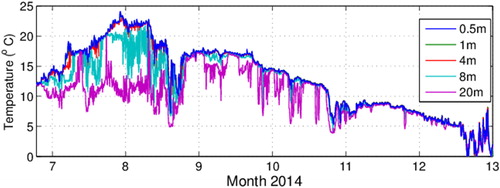
The annual average cycle of surface water temperature (WT) (measured at 5 m depth) shows a distinct seasonal cycle at the site, ranging from slightly above zero degrees in the late winter up to about 17 °C during summer (solid line in Fig. 5a). In addition, there is a strong interannual variability, in particular, during summer, when temperatures can reach up to 24 °C. Signatures of upwelling events are clearly visible between March and November (upwelling events are characterized as periods with distinctively lower WT and higher pCO₂; see Figs. 5a and c). An example of depth variation of water temperature from late June to December 2014 is shown in Fig. 6. During this year the uppermost water temperature (measured at 0.5 m) reaches 24 °C. With strong insolation during summer, there is typically a very shallow stratified layer near the surface, where the temperature also shows a diurnal cycle. With more moderate insolation there is generally a mixed layer between surface and 6–12 m depth during the summer season. In the winter, early spring and late fall the mixed layer is significantly deeper. Typical for the site are also variation on a shorter timescale, like upwelling (a signature of upwelling can be seen in late August in Fig. 6), diurnal variability and impacts of other mesoscale variations both in surface temperatures and at lower levels. The salinity ranges between 6.1 and 7.6 PSU and also displays a seasonal pattern, although with quite large year-to-year variations (Fig. 5b). Generally, the salinity is >6.8 PSU during the winter and <6.8 during the summer, but during short-term events, often coinciding with rapid WT decreases, salinity sometimes increases by <0.5 PSU. The surface pCO₂ ranges from <100 µatm to >1000 µatm and displays a clear seasonal cycle generally fluctuating between being oversaturated during fall and winter and undersaturated (<400 µatm) occurring during the spring and summer months (Fig. 5b). However, during short-term events pCO₂ can increase several hundred µatm and change from undersaturated to oversaturated conditions within one, or a few days. The oxygen saturation ranges from <70% to <130% in relation to atmospheric conditions and mirrors partly the pCO2 with undersaturated conditions from fall to spring and with oversaturation occurring during the summer months (Fig. 5d). However, in contrast to the pCO₂, the oxygen conditions during summer display larger year to year variations with rapid decreases in saturation (down to 70%) mainly occurring in May and July. Previous studies (e.g. Schneider et al., 2006; Omstedt et al., 2014) show two distinct minima in pCO₂ during summer in the Baltic Proper. These peaks are not as clear in the pCO₂ data at Östergarnsholm; rather, one extended period of low concentration occurs during summer (Fig. 5c). There are, however, two distinct maxima in oxygen during summer (Fig. 5d).

Fig. 5. Annual cycle of (A) WT, (B) salinity, (C) pCO₂ and (D) oxygen saturation measured during 2005–2016 for WT and pCO₂, and during 2011–2016 for salinity and oxygen saturation at the Östergarnsholm site. Grey dots are individual measured data, solid black line is average value. Dashed lines represent current equilibrium with the atmosphere for CO₂ and 100% saturation for oxygen. The sensors were placed at 5 m depth. Position of sensors is indicated by SAMI sensor in Figure 1.

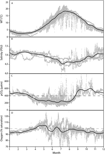
Fig. 6. Water temperatures at the 5 measuring depths (0.5–20 m) from late June to late December 2014 (decimal month is shown in the figure).

The TP and TN concentrations collected in the three depth profiles near the sensor-mooring are relatively homogeneous throughout the profile (Table 2). The variability between depths for both NO₃ and NH₄ is much larger, also with large variability over time, as shown by the high standard deviations. For PO₄ and DSi the highest concentrations were observed near the bottom and with relatively low variability over time. The concentrations for TP, TN, PO₄ and NO₃ + NH₄ are within the range previously reported for the Baltic Proper (HELCOM, 2009).

Table 2. Mean water chemistry based on monthly sampling during April to November 2016 at three different depths at the Östergarnsholm site.

Depth (m)	pH	TN	NO3-N	NH4-N	TP	PO4-P	DSi
0.5	8.1 (0.1)	21.5 (6.2)	0.7 (1.0)	3.1 (4.5)	0.61 (0.1)	0.24 (0.2)	13.5 (1.8)
10	8.0 (0.1)	19.5 (2.5)	0.6 (1.0)	1.9 (1.4)	0.59 (0.1)	0.27 (0.1)	13.8 (1.8)
18	8.0 (0.1)	20.6 (4.3)	0.8 (0.9)	2.6 (3.0)	0.63 (0.1)	0.31 (0.1)	14.7 (1.9)

All data except for pH is in the unit of µmol/L. Standard deviations are given within brackets.

5.2. Surface roughness and heat fluxes

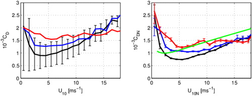
Sea surface roughness or drag can be characterized by the drag coefficient $C_D={\left(\frac{u_{*}}{U_{10}}\right)}^2,$ where U₁₀ is the wind speed at 10 m above the surface and u_* the friction velocity. The drag coefficient and wind speed can be normalized to the corresponding neutral atmospheric stratification and are then denoted C_DN and U_10N, respectively. Data from Östergarnsholm for the period 2013 to 2015 are used to calculate the drag coefficient and the dependence of the wind speed (in total 14,580 60 min data), and the same data are used to estimate the stability parameter. In Fig. 7 C_D and C_DN averaged over wind-speed intervals are shown representing data for the different categories defined in Table 1. In Fig. 7a the black curve (representing open sea conditions; CAT1) are shown with one standard deviation (σ) representing the scatter of the data. The scatter for the coastal sea (CAT2; blue) and mixed land–sea (CAT3; red) is significantly larger compared to open sea data, due to the larger variability of data in these sectors (variability of CAT2 and CAT3 not shown). In Fig. 7b the neutral drag coefficient is shown, and for comparison the drag coefficient calculated from wind speed using the Charnock relation ($z_0=\alpha \frac{u_{*}^2}{g}$) (Charnock, 1955) with the Charnock constant α = 0.0185 (green curve). Here z₀ is the roughness length and g acceleration of gravity. The value of the Charnock coefficient is frequently used in many applications, and originates from Wu (1980). The error bars in 7 b represent $\frac{\sigma }{\sqrt{N}},$ where N is the total number of data points for the respective interval; this illustrates the significance of the differences between the curves. The open sea drag coefficient (or roughness length) is expected to also depend on the wave conditions, defined by wave age and/or wave steepness. Wave age divides between a wind sea with growing sea conditions and a swell-dominated wave field. In pure wind-sea cases these conditions are mainly defined by wind speed, but in mixed seas and swell-dominated seas the situation is different (e.g. Taylor and Yelland, 2001; Smedman et al., 2003; Guan and Xie, 2004; Drennan et al., 2005; Potter, 2015). This is an important aspect of analysing the data, but beyond the scope of this study. The open sea drag coefficient estimated at Östergarnsholm is lower on the average compared to using the Charnock equation, in agreement with previous studies, for example, Carlsson et al. (2009), showing a reduction of the neutral drag coefficient during swell-dominated conditions in the Baltic Sea. Swell conditions are frequent in the Baltic Sea and will result in a lower average drag coefficient compared to open ocean data. The drag coefficient calculated using data representing the coastal zone (Fig. 7, blue curves) is larger compared to open sea data; this is particularly clear for winds below 10 m/s. The higher drag coefficient for data representing the near-coastal region agrees with previous studies where fetch-limited conditions give enhanced surface drag (e.g. Geernaert, 1988). When the flow is partly over the shoreline, the drag could be expected to be even larger due to the partial influence of the rougher land surface. This is not seen in our data; there are, however, relatively small number of data points for this sector (CAT3 data). It is interesting to note that there is less wind-speed dependence for the coastal and mixed land–sea sector (CAT2 and CAT3), and C_DN is approximately the same for the different sectors (different categories) for wind speeds over 15 m/s. For the low wind speeds the drag coefficient is increasing. This agrees with other studies for open sea data, and here a similar trend is shown for coastal and mixed sea/land data. This is also a prominent feature at land sites (Mahrt et al., 2001), where it is argued that C_D decreases at higher wind speed due to a streamlining effect.

Fig. 7. Drag coefficient averaged over wind-speed intervals, error bars show one standard deviation of the variability of CAT1; for clarity of the figure, variability is not shown for the other sectors, being larger than for CAT1, (a) and corresponding neutral drag coefficient; error bars show $\frac{\sigma }{\sqrt{N}}$ (b). Black lines represent open sea sector (CAT1), blue lines coastal sector (CAT2) and red lines mixed land–sea sector (CAT3). Green line in (b) is the drag coefficient calculated using Charnock equation. Data are from 2013 to 2015.

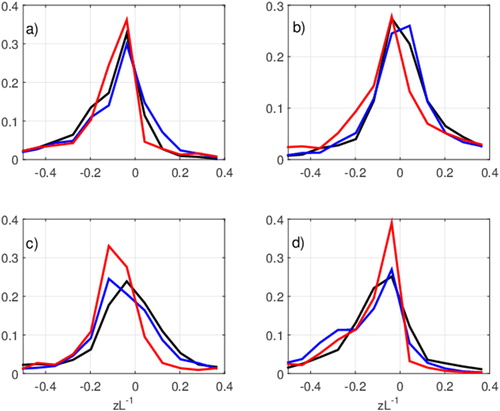
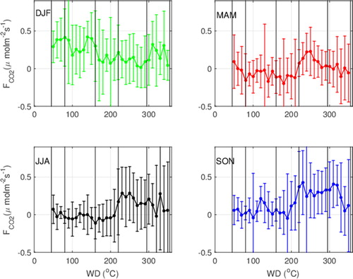
The atmospheric stability parameter, ζ, is used to determine the dominance of unstable or stable atmospheric stratification. It is defined as $$\zeta =\frac{z}{L}=\frac{zg\kappa \overline{w\prime t\prime }}{u_{*}^{3}T}$$ where L is the Monin-Obukhov length, z is the measuring height, κ the von Kármán constant, w´t´ the buoyancy flux and T the atmospheric temperature. The frequency distribution of ζ is shown for the different seasons in Fig. 8. Seasons are defined as winter (DJF; December, January, February), spring (MAM; March, April, May), summer (JJA; June, July, August) and fall (SON; September, October, November). Compared to most open ocean data we see a relatively high frequency of stable atmospheric stratification (negative buoyancy flux and positive ζ); this is true for all seasons, but particularly for spring and summer. Near neutral or slightly unstable data are most common on an annual basis, and for the fall and winter seasons for all data categories. The data from the coastal sector are more shifted to unstable during fall; this reflects the air–sea temperature difference being large during fall, where the colder air from the nearby land areas is advected over the relatively warm water for the coastal sector. Due to the higher heat content in deeper waters, unstable stratification prevails during winter for the data representing the open sea sector. For spring and summer, the data in the coastal sector are more shifted to stable stratification during spring and for open sea during summer. This reflects the warmer air originating from nearby land areas, advected over the colder sea surface for the coastal sector during spring. During summer the slow warming of the water in the open sea sector results in relatively low WT and stable stratification for the open sea sector. There are relatively few data in the land–sea mixed sector; the data are generally shifted to more unstable stratifications compared to the other data.

Fig. 8. Frequency distribution of the stability parameter z/L for the different data categories for (a) winter (DJF), (b) spring (MAM), (c) summer (JJA) and (d) fall (SON). Black lines represent open sea sector (CAT1), blue coastal sector (CAT2) and red mixed land–sea sector (CAT3). Data are from 2013 to 2015.

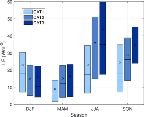
High frequency data of stable atmospheric stratification agrees with previous studies for the site (Svensson et al., 2016) and most likely more common in the Baltic Sea compared to open ocean conditions. For sensible and latent heat fluxes data from January 2015 to December 2017 are used (a total of 11,377 30 min data). A similar picture is seen in the seasonally mean sensible heat flux data (H, Fig. 9), where negative fluxes (downward) are seen in spring and summer for CAT1 and CAT2 data and positive fluxes during fall and winter. The scatter is generally higher for the coastal data. Low CAT2 heat flux data in winter can be explained by Fig. 10a, where upward fluxes (from sector 45°<WD < 80°) and downward fluxes (from sector 220°<WD < 295°) to some extent average out. For latent heat fluxes (Fig. 11) the CAT2 data show relatively large evaporation during summer and fall. Evaporation during fall is largest for all sectors and smallest during spring. Negative latent heat fluxes occur, but are not very frequent. Large evaporation in the coastal area is explained by breaking waves in the shallower water and by large air–sea temperature and humidity differences. Large evaporation during fall is mainly explained by relatively high water temperatures and to some extent high wind speeds (Fig. 10d); small evaporation during spring is due to low water temperatures, relatively low wind speeds and stable atmospheric stratification.

Fig. 9. Seasonally averaged sensible heat flux for the different category data (CAT1, CAT2 and CAT3, respectively). The boxes are defined based on the first and third quartile of the distribution and thus show the interquartile range corresponding to 50% of the data; the circles are the mean, and thin horizontal lines the median. Number of data items for each of the boxes ranges from 500 to1800 for CAT1 and CAT 2 and from 130 to 355 for CAT3.

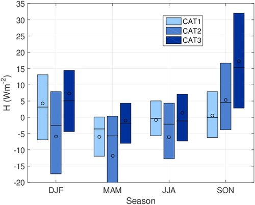
Fig. 10. Bin (interval) averages of (a) sensible heat flux, (b) latent heat flux, (c) friction velocity and (d) wind speed. Lines represent winter DJF (green), spring MAM (red), summer JJA (black) and fall SON (blue). Thin vertical lines represent wind direction intervals according to Table 1.

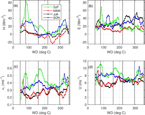
Fig. 11. Seasonally averaged latent heat flux for the different category data. Boxes’ representation and number of data as in Figure 9.

5.3. Gas fluxes

There is a clear seasonal variation in the direction of the CO₂ flux (Fig. 12). For the open sea sector, uptake is dominating during spring, summer and fall. For CO₂ fluxes, data from January 2015 to December 2017 are used (same data set as sensible and latent heat fluxes). During winter, outgassing is dominating for CAT1 data, and relatively large magnitudes of the fluxes (large fluxes due to the higher winds during winter season; see also Fig. 10d for the wind speeds and corresponding friction velocities, Fig. 10c). The seasonal cycle of CAT1 data agrees qualitatively with results from other studies of air–sea CO₂ flux for open Baltic Sea conditions (e.g. Norman et al., 2013; Parard et al., 2017). The open sea sector has in general the highest frequency of small magnitude fluxes, probably due to the smallest air–sea CO₂ gradients. The data for the coastal sector (CAT2) show outgassing as a seasonal mean for all seasons (during spring, uptake and outgassing balances out on the average) and largest during fall. This has most likely two explanations: the coastal sector is influenced by runoff, with water of high carbon content leading to an oversaturation of pCO₂ and an upward directed flux. The coastal sector is also the sector where the upwelling has the largest impact, bringing carbon-rich water from large depths to the surface. One could also expect biological activities to be high in the coastal sector, and thus large uptake during spring and summer. The mixed land–sea sector shows a high frequency of fluxes with a large magnitude (positive or negative), in particular, during fall and winter seasons. The mixed land–sea sector is influenced by high biological activities in the shore areas, run-off and also biological processes on land. One could thus expect other factors (such as radiation and diurnal cycle) influencing the direction and magnitude of the flux and explaining the large variability. The fluxes are shown for different wind directions in Fig. 13. During fall, there are relatively large fluxes in the wind direction sector 200°–240°; this can be interpreted as a signature of upwelling, which brings cold, CO₂-rich water to the surface. Upwelling occurs relatively frequently during fall for this wind direction (Lehmann et al., 2012). There are indications of upwelling signals also during spring and summer with slightly higher average CO₂ fluxes for wind directions from 200°–220° compared to 160°–200°, but not as clear as during fall.

Fig. 12. Seasonally averaged flux of carbon dioxide for the different category data. Note here the difference in wind direction ranges for physical and biogeochemical parameters for the different categories. Boxes’ representation as in Figure 9. Number of data for each of the box ranges from 100 to 600 for CAT1, 1300 to 2700 for CAT 2 and 130 to 355 in CAT3.

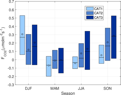
Fig. 13. Flux of carbon dioxide (in μmolm⁻²s⁻¹) averaged over wind direction intervals. Error bars represent one standard deviation of the data in the respective interval. Vertical black lines indicate limitation for wind direction intervals following Table 1.

When suggesting the sectors for the different data categories (Section 4.1.6), data with winds from the sector 160°–220° were defined as CAT1 for physical properties and CAT2 for biogeochemical properties (i.e. CAT P1/B2). With the exception of winter, the fluxes are of similar magnitude for the 80°–160° and 160°–220° sectors. If filtering out the upwelling data and possible other coastal features (like situations with large run-off or biological activity), it might thus be possible to redefine the sector 160°–220° to CAT1 data also for biogeochemical properties (i.e. CAT P1/B1).

There are differences between the different sectors defined as CAT2 (CAT P2/B2, 45°<WD < 80° and 220°<WD < 295°). It is here possible that run-off and more direct land influence give large upward fluxes in the sector 220°–295° during spring, summer and fall.

5.4. Aerosol fluxes

Because aerosol deposition is a function of the aerosol concentration, one could expect downward flux to dominate the net flux, especially where we find the highest aerosol concentrations. At Östergarnsholm, this is in a wind sector corresponding to CAT P1/B1, where long-range transported aerosols from the European continent cause a broad peak in mean concentration of a few hundred particles cm⁻³ for the OPC and a few thousand particles cm⁻³ for the CPC. The lowest concentration is found in the northern and western wind sectors. This agrees with the aerosol climatology of northern Europe (Tunved et al., 2005). At a marine flux site as Östergarnsholm sea spray aerosol emissions are expected to play a dominant role (Nilsson et al., 2001; Geever et al., 2005). There are no local particle sources on Östergarnsholm, since the island is not inhabited, and there is enough vegetation to prevent significant dust emissions. To the east, here mostly corresponding to the eastern P2/B2 sector, many ship exhaust plumes from cargo traffic between St. Petersburg/Helsinki and the southern Baltic are observed, especially in the CPC aerosol concentration. Ship plumes give aerosol deposition during part of the half hour in which the plume passage occurs. Dry deposition of the long-range transported aerosol contributes to the net flux, so the aerosol flux values in Table 3 do not correspond to the total sea spray emissions.

Table 3. Aerosol fluxes for wind speeds above 4 m/s.

CAT	Compass	w’N’ CPC [m^–2s^–1]	w’N’ OPC [m^–2s^–1]
P2/B2	45°<WD < 80°	+9.84 × 10^5 (–1.17 × 10^6) –6.51 × 10^6 to +6.69 × 10^6	+1.81 × 10^5 (1.13 × 10^5) +2.68 × 10^4 to +2.93 × 10^5
P1/B1	80°<WD < 160°	+7.35 × 10^5 (+3.77 × 10^5) –8.39 × 10^6 to +1.04 × 10^7	+2.80 × 10^4 (+6.74 × 10^4) –1.19 × 10^5 to +1.71 × 10^5
P1/B2	160°<WD < 220°	–3.49 × 10^5 (+2.70 × 10^5) –2.65 × 10^6 to +2.63 × 10^6	+2.72 × 10^4 (+9.48 × 10^3) –7.18 × 10^4 to +8.88 × 10^4
P2/B2	220°<WD < 295°	+4.90 × 10^5 (+4.34 × 10^5) –1.79 × 10^6 to +2.00 × 10^6	+1.51 × 10^4 (+1.25 × 10^3) –4.73 × 10^4 to +4.82 × 10^4
P3/B3	295°<WD < 355°	–6.65 × 10^5 (–1.30 × 10^5) –2.70 × 10^6 to +2.18 × 10^6	+6.62 × 10^4 (+1.11 × 10^5) 2.60 × 10^4 to +1.30 × 10^5

Median (mean in parenthesis) and 25th–75th percentiles below. Red is max in its category, blue is min in its category.

The aerosol flux statistics in Table 3 show very clear differences between the different categories. In addition, the Table makes it clear that also from an aerosol flux point of view, the two P2/B2 sectors (45°<WD < 80° and 220°<WD < 295°) show great differences. Similarly, from the aerosol flux data, categories P1/B1 and P1/B2 appear to be very different from each other.

For the CAT 1 sectors, and the OCP size range, the median aerosol fluxes are upward and quite similar in the full sector (just below 3 × 10⁴ m⁻³s⁻¹), but the mean differs by nearly an order of magnitude, with the lower value for P1/B2. This is because of both overall small positive net fluxes as well as a large frequency of data points with negative net flux in P1/B2. The differences between these sectors are larger for the CPC fluxes (suggesting a larger difference in particles of diameters between 10 and 250 nm D_p than for D_p > 250 nm), where the median flux is 7.35 × 10⁵ m⁻³s⁻¹ and –3.49 × 10⁵ m⁻³s⁻¹, respectively, for CAT 1 P1/B1 and P1/B2.

For the OCP size range, the eastern P2/B2 sector is the one clearly most dominated by sea spray emissions. Negative OPC net fluxes in this sector are rare. For the CPC, the median flux is positive, while the mean is negative. This is because of a smaller number of data points with strong downward fluxes, which we associate with the ship exhaust plumes.

In the P3/B3 sector the OPC mean flux is as small as 1.11 × 10⁵ m⁻²s⁻¹, while the median is 6.62 × 10⁴ m⁻²s⁻¹. This is because of a large fraction of negative net fluxes in this sector. The shift towards negative fluxes is more evident for the CPC fluxes, where both mean and median fluxes are negative. This should imply a large influence of land surface in the flux footprint, which will both limit the sea spray influence and add dry deposition (dry deposition increases with increasing surface roughness). The CPC aerosol fluxes are more influenced, since at D_p < 250 nm the dry deposition should increase due to Brownian diffusion, and the OPC size range is dominated by the so-called accumulation mode where dry deposition is at a minimum.

Thus, over open sea in CAT 1, we find the largest sea spray emissions of about 10⁵ m⁻²s⁻¹. Overall, despite the wind sector categorization in Table 1 being made independent of the aerosol fluxes, the sectors show clearly different characteristics also in aerosol fluxes. From the open sea (especially from P1/B1) and from the easterly P2/B2 sector we have found an exponential increase in upward aerosol fluxes as a function of the wind speed, in agreement with previous studies in the Atlantic Ocean (Geever et al., 2005) and the Barents Sea/Arctic Ocean (Nilsson et al., 2001), although there are differences of the increase and in the magnitude.

6. Discussion

With a significantly longer response time to changes in atmospheric conditions of marine sites compared to terrestrial, surface atmosphere gradients are generally smaller and thus generate much smaller air surface fluxes. This puts large constraints on accuracy of the data. At terrestrial sites the surface energy balance is often used to control the quality of the data; this is not possible at marine sites, due to the slower and less local response of the water basins (in terms of temperature response as well as response of biogeochemical properties). Thus, quality control and evaluation of the site, the set-up and the data are highly important for marine micrometeorological sites. The flux footprint concept is crucial for micrometeorological sites (in particular, for land-based marine sites), and it is necessary to define the properties of the water in the footprint area of the tower. For data fulfilling open sea conditions one can expect relatively spatially homogeneous conditions, and one marine station can represent a relatively large area. This is, however, not the case for the coastal zone or shore areas with land influence, where the variability is much larger. One could thus argue for the use of micrometeorological methods for monitoring CO₂ fluxes in coastal areas, as they also represent an integrated estimate for very heterogeneous footprints. Additional problems (not included in the present study) for land-based air–sea interaction sites are the measurement of parameters where the footprint concept is not relevant (i.e. upward radiative components or pressure fluctuations). The sensor needs to reach far out from the shore to measure the relevant water surface properties. For land-based sites, generally a broader range of conditions (in terms of air–sea gradients) occur, due to land–sea contrast and coastal features, and one could consider them as large-scale open sea laboratories.

One needs, however, to be careful when using data during very stable atmospheric conditions. Simplified modelling indicates a reduction of vertical fluxes due to upwind disturbances caused by land areas, being stronger for high and steep coastlines.

Because the eastern P2/B2 sector shows the largest upward aerosol fluxes of all sectors, especially in the OPC size range, even larger than in the P1/B1 sector, one could assume that some process(es) enhance(s) sea spray emissions in this sector. The most likely explanation would be that wave breaking is more intense in shallow water, and with that, a large production of sea spray (see Section 3.14 above on wave field characteristics at the station).

The dominance of negative fluxes in the P3/B3 sector for the CPC aerosol fluxes shows that aerosol flux measurements can also be a valuable contribution to interpretation of meteorological fluxes and gas fluxes. Presuming that there are no or few local aerosol sources, as on Östergarnsholm, land will only contribute negative aerosol fluxes, while the aerosol fluxes over sea surfaces will be dominated by upward fluxes from sea spray emissions. That implies that land surfaces within the footprint will rapidly show up as a shift from upward to downward fluxes.

7. Conclusions

There is a great potential in using land-based micrometeorological stations, both for monitoring of ocean and coastal conditions and for understanding of air–sea interaction processes. For land-based sites some land impact is unavoidable, but for high quality flux data it is important to classify and clearly quantify the land impact. We suggest a methodology to distinguish defined categories for the data from marine land-based measuring sites. We suggest distinguishing characterization of physical parameters (momentum, heat and aerosol fluxes) from biogeochemical fluxes. Suggested categories for ice-free seas are

• CAT1: Open sea, marine station, a wave field undisturbed by topographical or coastal features, water-side measuring system representative of the flux footprint of the tower. Mesoscale circulation system in the sea or the atmosphere might influence the station, but the data can be considered stationary and homogeneous. The aerosol flux is dominated by sea spray emissions.

• CAT2: Coastal sea, a local wave field influenced by bathymetry or limited fetch, resulting in physical properties different from open sea conditions or strong gradients of temperature and salinity in the footprint region due to the water depth. In a near-surface region the biogeochemical properties can vary, even if the physical ones do not. This can originate from differences in DOC due to run-off or variation in biological activity in the vicinity of land and shallower water. In the eastern CAT2 sector we observed a stronger contribution from sea spray emissions than from the CAT1 sector, suggesting that shallow water influence on the wave breaking enhanced sea spray formation.

• CAT3: Mixed land–sea, mixed land–sea footprint of the tower with very heterogeneous physical and biogeochemical conditions, where it is not possible to fully represent water-side conditions, with only few water-side measurements. Because aerosol fluxes are dominated by dry deposition over land and by sea spray emissions over land, we see the turbulent aerosol fluxes change sign when the footprint includes land surface as in CAT 3. In that way aerosol fluxes could help characterize similar sectors for other land-based marine flux stations. The work involved in this would only consist of (a) removing all episodes of local combustion aerosols, a process which always is necessary, anyway, when studying natural aerosol sources, and (b) disregarding wind sectors with light dry sand that could contribute upward local dust sources. Especially on sites with no or little sand in the local footprint, aerosol fluxes could then serve as a complement to traditional momentum flux-based methods to separate land from sea.

When using the suggested categorization for data taken at the well-studied Östergarnsholm site in the Baltic Sea, we find a larger variability in surface drag, heat and CO₂ fluxes for mixed land–sea and coastal data compared to open sea conditions. This is due to the greater heterogeneity of surface water and atmospheric conditions. The drag coefficient is largest (at least for winds below 10 m/s) for the mixed land–sea data and smallest for open sea conditions; the larger drag for the coastal sector can probably be explained by more strongly forced and generally steeper waves. The seasonal cycle of CO₂ flux is different for the data from the different categories where open sea data show uptake during spring and summer. Coastal and mixed land–sea data show outgassing during all seasons, probably due to impact of run-off of high DOC concentrations in the water. It should be noted that upwelling signals are seen during several seasons.

For an improved understanding of the air–sea interaction in coastal regions we suggest combining different coastal sites, as the variation between the sites contributes to understanding processes in the coastal ocean and marginal seas. For such a comparison between sites to be fruitful, a characterization of the properties of the flux footprints for different wind directions would be valuable. The suggested characterization presented here could be one methodology to implement.

Acknowledgements

Present and previous staffs working at the Östergarnsholm station and data are gratefully acknowledged for valuable contributions. Reviewers are acknowledged for valuable comments improving the manuscript.

Disclosure statement

No potential conflict of interest was reported by the authors.

Additional information

Funding

The work of H. Pettersson was partly supported by ENVRIplus/EoP project (European Commission, project reference number 654182). The ICOS station Östergarnsholm is funded by Swedish Research Council and Uppsala University. L. Wu is supported by the Swedish Research Council (project 2012-3902). The aerosol flux measurements by Stockholm University were funded by Vetenskapsrådet (Swedish Research Council) projects MASC (Influence of marine microbiology on sea spray aerosol, cloud and climate) 2010-3821 and CESSA (Climate Effects of Sea Spray Aerosols) 2014-5354, and FORMAS (Swedish Research Council for Environment, Agricultural Science and Spatial Planning) project 2007-1362 (Seasonal variation in the primary marine aerosol source due to physical and bio/chemical processes). This work forms part of the BONUS INTEGRAL project.

References

- Ahlm, L., Krejci, R., Nilsson, E. D., Mårtensson, E. M., Vogt, M. and co-authors. 2010. Emission and dry deposition of accumulation mode particles in the Amazon Basin. Atmos. Chem. Phys. 10, 10237–10253. doi:10.5194/acp-10-10237-2010
- Ahlm, L., Nilsson, E. D., Krejci, R., Mårtensson, E. M., Vogt, M. and co-authors. 2010. A comparison between dry and wet season aerosol number fluxes over the Amazon rain forest. Atmos. Chem. Phys. 10, 3063–3079. doi:10.5194/acp-10-3063-2010
- Anctil, F., Donelan, M. A., Drennan, W. M. and Graber, H. C. 1994. Eddy-correlation measurements of air-sea fluxes from a discus buoy. J. Atmos. Oceanic Technol. 11, 1144–1150. doi:10.1175/1520-0426(1994)011<1144:ECMOAS>2.0.CO;2
- Anderson, K., Brooks, B., Caffre, P., Clarke, A., Cohen, L. and co-authors. 2004. The RED experiment—An assessment of boundary layer effects in a trade winds regime on microwave and infrared propagation over the sea. Bull. Am. Meteorol. Soc. 85, 1355–1365. doi:10.1175/BAMS-85-9-1355
- Aubinet, M., Vesala, T. and Papale, D. 2012. Eddy Covariance: A Practical Guide to Measurements and Data Analysis. Springer Atmospheric Sciences Series, Springer, 436 pp.
- Baldocchi, D. D. 2003. Assessing the eddy covariance technique for evaluating carbon dioxide exchange rates of ecosystems: Past, present and future. Glob. Change Biol. 9, 479–492. doi:10.1046/j.1365-2486.2003.00629.x
- Buzorius, G., Rannik, Ü., Nilsson, E. D. and Kulmala, M. 2001. Vertical fluxes and micrometeorology during the new aerosol particle formation. Tellus B 53, 394–405. doi:10.3402/tellusb.v53i4.16612
- Carlsson, B., Rutgersson, A. and Smedman, A. 2009. Impact of swell on simulations using a regional atmospheric climate model. Tellus A 61, 527–538.
- Charnock, H. 1955. Wind stress on a water surface. Q. J. R. Meteorol. Soc. 81, 639–640. doi:10.1002/qj.49708135027
- Chen, C. T. A., Huang, T. H., Chen, Y. C., Bai, Y., He, X. and co-authors. 2013. Air-sea exchanges of CO2 in the world’s coastal seas. Biogeosciences 10, 6509–6544. doi:10.5194/bg-10-6509-2013
- DeCosmo, J., Katsaros, K. B., Smith, S. D., Anderson, R. J., Oost, W. A. and co-authors. 1996. Air-sea exchange of water vapor and sensible heat: The humidity exchange over the sea (HEXOS) results. J. Geophys. Res. 101, 12001–12016. doi:10.1029/95JC03796
- Drennan, W. M., Taylor, P. K. and Yelland, M. J. 2005. Parameterizing the sea surface roughness. J. Phys. Oceanogr. 35, 835–848. doi:10.1175/JPO2704.1
- Engler, C., Lihavainen, H., Komppula, M., Kerminen, V.-M. and Kulmala, M. 2007. Continuous measurements of aerosol properties at the Baltic Sea. Tellus B 59, 728–741. doi:10.1111/j.1600-0889.2007.00285.x
- Fairall, C., Hare, J., Edson, J. and McGillis, W. 2000. Parameterization and micrometeorological measurements of air-sea gas transfer. Boundary Layer Meteorol. 96, 63–105. doi:10.1023/A:1002662826020
- Garbe, C. S., Rutgersson, A., Boutin, J., Delille, B., Fairall, C. W. and co-authors. 2014. Transfer across the air–sea interface. In Ocean-Atmosphere Interactions of Gases and Particles (eds. P. S. Liss and M. T. Johnson). Springer, New York, pp. 55–112.
- Gattuso, J.-P., Frankignoulle, M. and Wollast, R. 1998. Carbon and carbonate metabolism in coastal aquatic ecosystems. Annu. Rev. Ecol. Syst. 29, 405–434. doi:10.1146/annurev.ecolsys.29.1.405
- Geernaert, G. 1988. Drag coefficient modeling for the near coastal zone. Dyn. Atmos. Oceans 11, 307–322. doi:10.1016/0377-0265(88)90004-8
- Geever, M., O’Dowd, C., van Ekeren, S., Flanagan, R., Nilsson, E. D. and co-authors. 2005. Sub-micron sea-spray fluxes. Geophys. Res. Lett. 32, L15810.
- Griessbaum, F. and Schmidt, A. 2009. Advanced tilt correction from flow distortion effects on turbulent CO2 fluxes in complex environments using large eddy simulation. Q. J. R. Meteorol. Soc. 135, 1603–1613. doi:10.1002/qj.472
- Grönlund, A., Nilsson, D., Koponen, I. K., Virkkula, A. and Hansson, M. E. 2002. Aerosol dry deposition measured with eddy-covariance technique at Wasa, Dronning Maud Land, Antarctica. Ann. Glaciol. 35, 355–361. doi:10.3189/172756402781816519
- Guan, C. and Xie, L. 2004. On the linear parameterization of drag coefficient over sea surface. J. Phys. Oceanogr. 34, 2847–2851. doi:10.1175/JPO2664.1
- HELCOM. 2009. Eutrophication in the Baltic Sea – An integrated thematic assessment of the effects of nutrient enrichment and eutrophication in the Baltic Sea region. Baltic Sea Environment Proceedings. No. 115B, Helsinki Commission, 148 pp.
- Högström, U., Sahlée, E., Drennan, W. M., Kahma, K. K., Smedman, A.-S. and co-authors. 2008. Momentum fluxes and wind gradients in the marine boundary layer – A multi platform study. Boreal Env. Res. 13, 475–502.
- Källstrand, B., Bergström, H., Højstrup, J. and Smedman, A.-S. 2000. Meso-scale wind field modifications over the Baltic Sea. Boundary Layer Meteorol. 95, 161–188. doi:10.1023/A:1002619611328
- Landwehr, S., Miller, S. D., Smith, M. J., Saltzman, E. S. and Ward, B. 2014. Analysis of the PKT correction for direct CO2 flux measurements over the ocean. Atmos. Chem. Phys. 14, 3361–3372. doi:10.5194/acp-14-3361-2014
- Landwehr, S., Sullivan, N. O. and Ward, B. 2015. Direct flux measurements from mobile platforms at sea: Motion and airflow distortion corrections revisited. J. Atmos. Oceanic Technol. 32, 1163–1178. doi:10.1175/JTECH-D-14-00137.1
- Leclerc, M. Y. and Foken, T. 2014. Foot-Prints in Micrometeorology and Ecology. Vol. XIX. Springer, Heidelberg, 239 pp.
- Lee, X., Massman, W. and Law, B. 1998. Handbook of Micrometeorology. Vol. XIV. Springer, Netherlands, 250 pp.
- Lehmann, A., Myrberg, K. and Höflich, K. 2012. A statistical approach to coastal upwelling in the Baltic Sea based on the analysis of satellite data for 1990–2009. Oceanologia 54, 369–339. doi:10.5697/oc.54-3.369
- Mahrt, L., Vickers, D., Sun, J., Jensen, N. O., Jørgensen, H. and co-authors. 2001. Determination of the surface drag coefficient. Boundary Layer Meteorol. 99, 249–276. doi:10.1023/A:1018915228170
- Miller, S. D., Marandino, C. and Saltzman, E. S. 2010. Ship-based measurement of air-sea CO2 exchange by eddy covariance. J. Geophys. Res. 11, D02304.
- Muller-Karger, F. E., Varela, R., Thunell, R., Luerssen, R., Hu, C. and co-authors. 2005. The importance of continental margins in the global carbon cycle. Geophys. Res. Lett. 32, L01602,
- Neumann, T. and Nolopp, K. 2007. Three years operation of far offshore measurements at FINO1. DEWI Mag. 30, 42–46.
- Nilsson, E., Bergström, H., Rutgersson, A., Podgrajsek, E., Wallin, M. B. and co-authors. 2018. Evaluating humidity and sea salt disturbances on CO2 flux measurements. J. Atmos. Oceanic Technol. 35, 859–875. doi:10.1175/JTECH-D-17-0072.1
- Nilsson, E., Rutgersson, A. and Sullivan, P. 2010. Flux attenuation due to sensor separation over sea. J. Atmos. Oceanic Technol. 27, 856–868. doi:10.1175/2010JTECHA1388.1
- Nilsson, E. D. and Rannik, Ü. 2001. Turbulent aerosol fluxes over the Arctic Ocean: Part 1, dry deposition over sea and pack ice. J. Geophys. Res. 106, 32125–32137. doi:10.1029/2000JD900605
- Nilsson, E. D., Rannik, Ü., Swietlicki, E., Leck, C., Aalto, P. P. and co-authors. 2001. Turbulent aerosol fluxes over the Arctic Ocean: Part 2, wind driven sources from the sea. J. Geophys. Res. 106, 32139–32154. doi:10.1029/2000JD900747
- Norman, M., Parampil, S., Rutgersson, A. and Sahlée, E. 2013. Influence of coastal upwelling on the air-sea gas exchange of CO2 in a Baltic Sea Basin. Tellus B 65, 21831. doi:10.3402/tellusb.v65i0.21831
- O’Connor, T. C., Jennings, S. G. and O’Dowd, C. D. 2008. Highlights of fifty years of atmospheric aerosol research at Mace Head. Atmos. Res. 90, 338–355. doi:10.1016/j.atmosres.2008.08.014
- Omstedt, A., Humborg, C., Pempkowiak, J., Perttilä, M., Rutgersson, A. and co-authors. 2014. Biogeochemical control of the coupled CO2–O2 system of the Baltic Sea: A review of the results of BALTIC-C. AMBIO 43, 49–59. doi:10.1007/s13280-013-0485-4
- Parard, G., Rutgersson, A., Parampil, S. R. and Charantonis, A. A. 2017. The potential of using remote sensing data to estimate air-sea CO2 exchange in the Baltic Sea. Earth Syst. Dynam. 8, 1093–1106. doi:10.5194/esd-8-1093-2017
- Pedreros, R., Dardier, G., Dupuis, H., Graber, H. C., Drennan, W. M. and co-authors. 2003. Momentum and heat fluxes via the eddy correlation method on the R/V L'Atalante and an ASIS buoy. J. Geophys. Res. 108, 3339. doi:10.1029/2002JC001449
- Potter, H. 2015. Swell and the drag coefficient. Ocean Dyn. 65, 375–384. doi:10.1007/s10236-015-0811-4
- Prytherch, J., Yelland, M., Pascal, R., Moat, B., Skjelvan, I. and co-authors. 2010. Direct measurements of the CO2 flux over the ocean: Development of a novel method. Geophys. Res. Lett. 37, L03607.
- Rowe, M., Fairall, C. and Perlinger, J. 2011. Chemical sensor resolution requirements for near-surface measurements of turbulent fluxes. Atmos. Chem. Phys. 11, 5263–5275. doi:10.5194/acp-11-5263-2011
- Rutgersson, A., Norman, M., Schneider, B., Pettersson, H. and Sahlée, E. 2008. The annual cycle of carbon dioxide and parameters influencing the air–sea carbon exchange in the Baltic Proper. J. Mar. Syst. 74, 381–394. doi:10.1016/j.jmarsys.2008.02.005
- Rutgersson, A. and Smedman, A. 2010. Enhancement of CO2 transfer velocity due to water-side convection. J. Mar. Syst. 80, 125–134. doi:10.1016/j.jmarsys.2009.11.004
- Rutgersson, A., Smedman, A. and Omstedt, A. 2001. Measured and simulated latent and sensible heat fluxes at two marine sites in the Baltic Sea. Boundary Layer Meteorol. 99, 53–84. doi:10.1023/A:1018799227854
- Rutgersson, A., Smedman, A. and Sahlée, E. 2011. Oceanic convective mixing and the impact on air-sea gas transfer velocity. Geophys. Res. Lett. 38, L02602.
- Sahlée, E., Smedman, A., Högström, U. and Rutgersson, A. 2008. Re-evaluation of the bulk exchange coefficient for humidity at sea during unstable and neutral conditions. J. Phys. Oceanogr. 38, 257–272. doi:10.1175/2007JPO3754.1
- Sahlée, E., Smedman, A., Rutgersson, A. and Högström, U. 2008. Spectra of CO2 and water vapour in the marine atmospheric surface layer. Boundary Layer Meteorol. 126, 279–295. doi:10.1007/s10546-007-9230-5
- Schack, C. J., Jr., Pratsinis, S. E. and Friedlander, S. K. 1985. A general correlation for deposition of suspended particles from turbulent gases to completely rough surfaces. Atmos. Environ. 19, 953–960. doi:10.1016/0004-6981(85)90240-9
- Schneider, B., Kaitala, S. and Maunula, P. 2006. Identification and quantification of plankton bloom events in the Baltic Sea by continuous pCO2 and chlorophyll a measurements on a cargo ship. J. Mar. Syst. 59, 238–248. doi:10.1016/j.jmarsys.2005.11.003
- Smedman, A., Högström, U., Bergström, H., Rutgersson, A., Kahma, K. and co-authors. 1999. A case-study of air-sea interaction during swell conditions. J. Geophys. Res. 104, 25833–25851. doi:10.1029/1999JC900213
- Smedman, A.-S., Guo Larsén, X., Högström, U., Kahma, K. K. and Pettersson, H. 2003. Effect of sea state on the momentum exchange over the sea during neutral conditions. J. Geophys. Res. 108, 2156–2202.
- Smith, S. D. 1980. Wind stress and heat flux over the ocean in gale force winds. J. Phys. Oceanogr. 10, 709–726. doi:10.1175/1520-0485(1980)010<0709:WSAHFO>2.0.CO;2
- Sproson, D. and Sahlée, E. 2014. Modelling the impact of Baltic Sea upwelling on the atmospheric boundary layer. Tellus A 66, 24041. doi:10.3402/tellusa.v66.24041
- Svensson, N., Sahlée, E., Bergström, H., Nilsson, E., Badger, M. and Rutgersson, A. 2017. A case study of offshore advection of boundary layer rolls over a stably stratified sea surface. Advances in Meteorology. 2017. doi:10.1155/2017/9015891
- Svensson, N., Bergström, H., Sahlée, E. and Rutgersson, A. 2016. Stable atmospheric conditions over the Baltic Sea: Model evaluation and climatology. Boreal Environ. Res. 21, 387–404.
- Takahashi, T., Olafsson, J., Goddard, J. G., Chipman, D. W. and Sutherland, S. C. 1993. Seasonal-variation of CO2 and nutrients in the high-latitude surface oceans—A comparative study. Glob. Biogeochem. Cycles 7, 843–878. doi:10.1029/93GB02263
- Taylor, P. K. and Yelland, M. J. 2001. The dependence of sea surface roughness on the height and steepness of the waves. J. Phys. Oceanogr. 3, 572–590.
- Tunved, P., Nilsson, E. D., Hansson, H.-C. and Ström, J. 2005. Aerosol characteristics of air masses in Northern Europe: Influence of location, transport, sinks and sources. J. Geophys. Res. 110, 7201.
- Vesala, T., Kljun, N., Rannik, Ü., Rinne, J., Sogachev, A. and co-authors. 2008. Flux and concentration footprint modelling: State of the art. Environ. Pollut. 152, 653–666. doi:10.1016/j.envpol.2007.06.070
- Vickers, D. and Mahrt, L. 2003. The cospectral gap and turbulent flux calculations. J. Atmos. Oceanic Technol. 20, 660–672.
- Vogt, M., Nilsson, E. D., Ahlm, L., Mårtensson, E. M. and Johansson, C. 2011. The relationship between 0.25–2.5 μm aerosol and CO2 emissions over a city. Atmos. Chem. Phys. 11, 4851–4859. doi:10.5194/acp-11-4851-2011
- Webb, E., Pearman, G. and Leuning, R. 1980. Correction of the flux measurements for density effects due to hear and water vapour transfer. Q. J. R. Meteorol. Soc. 106, 85–100. doi:10.1002/qj.49710644707
- Wu, J. 1980. Wind-stress coefficients over sea surface near neutral conditions—A revisit. J. Phys. Oceanogr. 10, 727–740. doi:10.1175/1520-0485(1980)010<0727:WSCOSS>2.0.CO;2
- Yang, M., Bell, T. G., Hopkins, F. E., Kitidis, V., Cazenave, P. W. and co-authors. 2016. Air–sea fluxes of CO2 and CH4 from the Penlee Point Atmospheric Observatory on the south-west coast of the UK. Atmos. Chem. Phys. 16, 5745–5761. doi:10.5194/acp-16-5745-2016