Global variability in radiative-convective equilibrium with a slab ocean under a wide range of CO₂ concentrations

Abstract

In radiative-convective equilibrium (RCE), radiative cooling of the troposphere is roughly balanced by the vaporization enthalpy set free by precipitating moist convection. Many earlier studies restricted the investigation of RCE to the dynamics of the atmosphere with constant boundary conditions including prescribed surface temperature. We investigate a GCM setup where a slab ocean is coupled to the atmosphere, and we explore a wide range of CO₂ concentrations. We obtain reliable statistical quantities from thousand-year-long simulations. For moderate CO₂ concentrations, we find unskewed temporal variations of 1–2 K in global mean surface temperature, with an almost constant climate sensitivity of 2 K. At CO₂ concentrations beyond four times the preindustrial value, the climate sensitivity decreases to nearly zero as a result of episodic global cooling events as large as 10 K. The dynamics of these cooling events are investigated in detail and shown to be associated with an increase in large-scale low-level stratiform cloudiness in the subsiding region, which is a result of penetrative shallow convection being capped by an inversion and thus not ventilating the lower troposphere. These dynamics depend on the CO₂ concentration: both through the effect of temperature on stratification and through the changing spatial scale of organization of the flow, which determines the spatial scale and temporal coherence of the stratiform cloud sheets.

Keywords:

• Radiative-convective equilibrium
• climate change
• cloud feedbacks
• global warming
• convective self-aggregation

1. Introduction

Radiative-convective equilibrium, or RCE, has established itself as an elegant model problem for exploring the leading-order energetic balance that determines Earth’s global climate. In this model problem, Earth is conceptualized as non-rotating with a homogeneous and usually water-covered surface, an initially homogeneous atmosphere, subject to a homogeneous insolation. Radiation destabilizes the atmosphere relative to the surface, which leads to precipitating deep convection. The vaporization enthalpy of water, which evaporates from the surface and condenses in the atmosphere, resolves the radiative imbalances in the two sub-systems, thereby establishing a radiative-convective equilibrium.

Early studies of RCE formulated the problem in one dimension, and provided the first compelling quantification of the sensitivity of the globally averaged surface temperature to increasing concentrations of atmospheric carbon dioxide (Manabe and Wetherald, 1967; Charney et al., 1979; Ramanathan and Coakley, 1978). The problem is increasingly studied using models designed to resolve the convective enthalpy transport, and thus encompassing more spatial dimensions (Nakajima and Matsuno, 1988; Held et al., 1993; Tompkins and Craig, 1998). These convective cloud-resolving models allow the atmospheric composition to develop spatial inhomogeneities, which are then balanced by circulations. These more fluid-dynamical formulations of RCE have produced surprising behavior, as despite the homogeneous framing of the problem, the spontaneous self-organization of convection – something called convective self-aggregation – influences the resultant equilibrium climate (Bretherton et al., 2005; Muller and Held, 2012). Many of the same features arise when studying convective self-aggregation in state-of-the-art climate models, and despite the necessity of parameterizing convective transports, large-scale circulations still develop (Popke et al., 2013; Arnold and Randall, 2015; Becker and Stevens, 2014; Bony et al., 2016; Coppin and Bony, 2015).

Most studies of RCE are performed with fixed sea-surface temperatures (SSTs). Fixed SSTs allow for a systematic analysis of how self-aggregation depends on the surface temperature. However, results show a strong model-dependency (Wing et al., 2017), both in convective cloud-resolving and climate models, which also motivated the currently ongoing RCEMIP project (Wing et al., 2018). Even though self-aggregation seems to be favored at higher temperatures in some models (e. g., Wing and Emanuel, 2014; Reed et al., 2015; Arnold and Randall, 2015), self-aggregation occurs across a wide range of SSTs (e. g., Wing and Cronin, 2016; Holloway and Woolnough, 2016) or with a non-linear dependence on SST in other models (e. g., Coppin and Bony, 2015; Becker et al., 2017). The analysis of simulations with fixed SSTs also led to some questions as to whether RCE is a well-posed problem. In a series of RCE experiments with a climate model, Becker et al. (2017) found that the radiative response at the top of the atmosphere to different fixed SSTs varied in unpredictable ways, raising the question as to whether the radiative response was a smooth function of the forcing. As the SST was increased, in some temperature ranges the net outgoing radiation decreased, which implies an unstable response to forcing. At other temperatures the opposite was the case. This behavior appeared to be related to differing degrees of convective self-aggregation, but the lack of a closed energy budget in simulations with fixed SSTs complicated attempts to understand this behavior.

This motivated us to return to the question of RCE using a slightly coarser resolution version of the model used by Becker et al. (2017), coupled to a slab ocean, which was shown by Hohenegger and Stevens (2016) to have a considerable impact on the dynamics. The coarser resolution allowed us to perform very long simulations and completely characterize the statistics of the equilibrium response of the system to forcing. The questions we were interested in answering were whether or not the model, in this very simple configuration, responded stably to perturbations of atmospheric CO₂, whether progressive doublings of atmospheric CO₂ were associated with predictably similar changes in surface temperature, and to what extent the imprint of convective self-aggregation manifests itself on the response of the system to forcing.

A wide array of simulations were performed. The CO₂ concentration was varied between 1/8th and 32-fold its pre-industrial value, and the insolation was varied by more than a factor of two about its present day value, both with and without a convective parameterization. Most simulations were run for around a thousand years and provide a stringent test of the physics of the climate model and the dynamics of its simulated climate. Stevens et al. (2019) give an overview of the simulations, and their sometimes surprising response to forcing. In this paper we study the equilibrium response of the simulations with the standard (parameterized convection) configuration of the model to changes in atmospheric CO₂ concentration, and only the most relevant subset of all CO₂ concentrations is used: whereas Stevens et al. (2019) demonstrated that the simulations responded smoothly to forcings varied modestly (± 10 W m⁻² about present-day values, albeit in ways that depended on how the model was configured), in this paper we attempt to understand the surprising dynamics of the system that emerge as the atmospheric concentration of CO₂ is increased, and which appears related to the development of convective self-aggregation.

The outline of the paper is as follows. In Section 2 nomenclature is introduced, and the numerical model and design of the experiments is described. In Section 3 the main features of the simulations as a function of CO₂ concentration are presented, with a primary focus on global-scale cooling events that progressively emerge as the concentration is increased. A hypothesis for the surprising behavior is also presented in this section. Support for the hypothesis is given in Section 4, where the dynamics of these events are explored in detail for the case of a 16-fold increase in atmospheric CO₂ concentration. Similar events that emerge at different values of atmospheric CO₂ concentrations are compared in Section 5. Reading the latter two sections is, however, not required to follow Section 6, where our main findings are restated and some of their implications are discussed. Relevant but inessential analyses are provided in a Supplemental Material.

2. The design of the numerical experiments

Simulations are performed with the general circulation model ECHAM6.3, version 6.3.02p4, which serves as the atmospheric component of the MPI-ESM1.2 (Mauritsen et al., 2019). To be able to run extremely long simulations, we use a coarse resolution, T31L47 (corresponding to 417 km zonally at the equator). All model settings of ECHAM6.3, including tuning constants, are the same as in the MPI-ESM1.2, with the exceptions as follows. The boundary conditions are RCE-specific and homogeneous, similar to those used by Popke et al. (2013) and Becker and Stevens (2014). Insolation is prescribed as spatially homogeneous, but temporally varying with a diurnal cycle (mean value: 340.3 W m⁻²). The Coriolis parameter is set to zero. The atmosphere is coupled to a perfectly vertically-conducting, fixed heat-capacity surface, which we refer to as a ‘slab ocean’. Through this boundary condition the slab-ocean temperature and the surface temperature are one and the same. The heat capacity chosen for the slab ocean corresponds to that of a water column of 25 m depth, which is half the value used in previous studies, so as to reduce the time it takes the system to equilibrate. All simulations are initialized from the same homogeneous dry initial state as in Becker et al. (2017), but with different initial slab ocean temperatures, depending on the respective CO₂ concentration and the expected equilibrium-state surface temperature.

We run the model for several different values of an assumed uniform concentration of atmospheric CO₂, which we denote by [CO₂]. The [CO₂] level is measured by the base-2 logarithm of the ratio of [CO₂] to a control value, which is taken to be that estimated for the pre-industrial atmosphere: (1) $$n={\hspace{0.17em}\text{log}\hspace{0.17em}}_2\left(\frac{\left[{\text{CO}}_2\right]}{278\text{ppm}}\right).$$(1)

When n is a natural number, it can be interpreted as the number of doublings. We analyze experiments for $n\in \{-1,0,1,2,2.5,3,3.5,4\},$ so that the highest [CO₂] reached corresponds to four doublings or 16 times more CO₂ than estimated for the pre-industrial atmosphere.

The PSrad implementation of the RRTM radiation scheme (Pincus and Stevens, 2013; Mlawer et al., 1997), which is used in the simulations, has been compared to line-by-line calculations, and performs reasonably even at the extreme CO₂ concentrations that we explore. Kluft et al. (2018) compute the clear-sky radiative forcing using the parent RRTM scheme, and show that its value at eight-times pre-industrial concentration (n = 3) is 15.45 W m⁻², compared to –4.57 W m⁻² for n = – 1. Were the forcing to increase by a constant factor for each doubling, the clear-sky radiative forcing would be 14.07 W m⁻² at n = 3, which is 10% less than the value it actually adopts in the model. This is a small effect and is consistent with the study by Gregory et al. (2015) who, using a different model, also show the forcing to increase more than linearly with n.

As mentioned above, to minimize sampling errors in estimates of statistical quantities, we carry out extremely long simulations, of the order of 10000 months; for the particular length for each setup, see Table 1. (The reason for the longer simulations for $n\ge 2$ are longer emerging time scales.) Because the simulations have no yearly cycle, and because the overturning time of the troposphere is of the order of a month, we adopt the month as the time unit, and present time non-dimensionalized by a unit month. Alternatively one could use the time scale for the ocean mixed layer to equilibrate, which for the 25 m-deep mixed layer used here corresponds to 120 months. It would be, however, too long to conveniently represent atmospheric processes.

Table 1. The length of the simulation in setups with different CO₂ concentration, characterized by the logarithm n of the CO₂ concentration relative to that of the control run (see Equation (1)(1) $$n={\hspace{0.17em}\text{log}\hspace{0.17em}}_2\left(\frac{\left[{\text{CO}}_2\right]}{278\text{ppm}}\right).$$(1) ).

n	–1	0	1	2	2.5	3	3.5	4
Length [months]	12180	11988	12300	17400	17400	17400	17400	17400

To find the longest time scale in the simulations, we analyzed the autocorrelation function of the global mean surface temperature. The longest decorrelation time to be identified by this analysis is around 400 months, and time scales that emerge in the subsequent analyses are typically much smaller than this, around 100 months at most. To ensure that we only analyze the simulations in a stationary state, we conservatively discard the first 2000 months, five times the longest decorrelation time that we found.

For all analyzed quantities, we take monthly means. This temporal resolution has proven sufficient to follow temporal variations, except for the diurnal cycle. The latter, however, is not identified as playing a direct role in any of the processes we study. It is also muted by the slab-ocean configuration, such that surface temperature variations on the diurnal time scale are typically small compared to the month-to-month variability.

3. Main properties of the equilibrium response for different CO₂ concentrations

3.1. Surface temperature evolution

We start exploring climate sensitivity by inspecting the time series of the global mean surface temperature, equivalently the temperature of the slab ocean, in setups with different [CO₂].

For modest changes in [CO₂], and as discussed in the introduction, the temperatures respond in a fashion consistent with expectation. This is shown in Fig. 1a, which presents time series of surface temperatures from four simulations, with n = –1, 0, 1, and 2. In this range, a higher concentration is strictly accompanied by warmer temperatures, and the temporal mean grows approximately linearly with n. This corresponds to a nearly constant climate sensitivity of approximately 2 K. Each setup exhibits internal variability of considerable strength, which is similar in the different setups, but for n = 1 and n = 2, periods of more pronounced cooling begin to appear (e.g. before t = 2700 and also near t = 3100 for n = 2).

Fig. 1. The global mean surface temperature as a function of time in setups with different CO₂ concentration, labeled by n. The temporal mean is also marked. The setup with n = 2 appears in both panels.

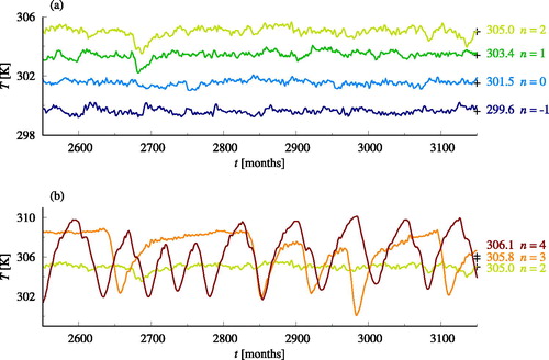
The episodic depressions in globally-averaged temperatures become increasingly pronounced at yet larger values of n. This is evident in the n = 3 and n = 4 temperature time series shown in Fig. 1b. For these cases the temperature even drops below the coldest values of the control run (n = 0). Beyond the growth of the amplitude, the frequency and the duration of the cooling events also increase for increasing [CO2]. While the temporal separation of subsequent cooling events is still erratic for n = 3, the events practically merge for n = 4 to form an uninterrupted oscillation with an approximate period determined by the duration of the individual events.

As a result of the growing importance of cooling episodes, the linear increase in the temporal mean surface temperature does not continue but seems to saturate (implying nearly zero climate sensitivity) for $2\le n\le 4.$ Simulations were performed also for n > 4, but for these temperatures increased more markedly and quickly reached values that were formally incompatible with assumptions in the model, causing the model to “crash”.

The characteristics described above can also be observed in Fig. 2, where two additional runs are included, with intermediate values of n. The distribution of the temperatures becomes strongly skewed for $n\ge 2,$ with a strong tail extending to low temperatures. This tail shows that the major temperature drops have a different nature compared to the minima of the fluctuations in the control run. At the same time, the upper bounds of the distributions are observed to grow approximately linearly with n, consistent with the expected response to the radiative effect of increasing [CO₂].

Fig. 2. Temporal statistics of the global mean surface temperature as a function of the logarithm n of the relative CO₂ concentration. Boxes represent the first quartile, the median, and the third quartile in time, and whiskers mark the temporal minimum and maximum. The temporal mean, with an error bar (see text), is included in blue next to the corresponding box.

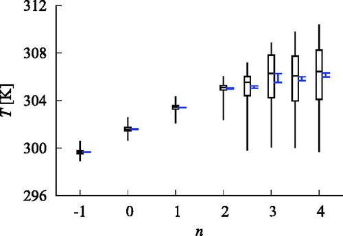
The temporal mean being smaller than the temporal median in Fig. 2 for high values of n is a further indication of the skewness of the distributions. Although possibly monotonic, the shape of the increase of the temporal mean as a function of the concentration is not trivial. This statement is substantiated by the small confidence intervals (for 95% confidence). These were obtained by temporally re-sampling the entire time series by shorter intervals, calculating the standard deviation of the temporal means in these samples, finding the one-over-the-square-root law as a function of the chosen length, and extrapolating it to the actual length of the entire time series.

3.2. Spatial structure

The other important impact of increasing the CO₂ concentration is the development of convective self-aggregation. Convective self-aggregation has been extensively studied using storm-resolving simulations (e.g. Bretherton et al., 2005; Muller and Held, 2012; Wing et al., 2017) and has also been shown to emerge in simulations of the global climate system under conditions of radiative-convective equilibrium (e.g. Becker and Stevens, 2014). In the majority of these studies, convection becomes more pronounced with increasing temperature (e.g. Arnold and Randall, 2015; Bony et al., 2016). Convection and subsidence, and hence the signature of self-aggregation, are most easily captured by the field of the vertical velocity ω (in pressure coordinates). For reasons that we explain in more depth in Section 4, instead of the traditional choice of investigating ω at the level of 500 hPa (e.g. Bony and Dufresne, 2005), we use values of ω at model level 41, ω₄₁, which locates at approximately 820 hPa, to look for signatures of convective self-aggregation.

For characterizing the size of the spatial structures of the ω₄₁ field, we evaluate, at each time instant, its spatial autocorrelation function C(α), defined as a function of the angular distance α (surface distance divided by the radius of the sphere) of two points on the spherical surface (Strube, 1985): for a given value of α, it is obtained by integrating over all point pairs on the sphere that are separated by α. This autocorrelation function thus characterizes spatial similarity on a sphere in an isotropic way.

The quantifier of the angular size of the spatial structures that has proven to be the most useful in our study is obtained from the first zero of the spatial autocorrelation function C(α). It corresponds to a standard definition of the integral length scale in turbulent flows (O’Neill et al., 2004) but is based on the vertical velocity only and is defined as follows: (2) $$S={\int }_0^{\alpha (C=0)}C(\alpha )\mathrm{d}\alpha .$$(2)

The temporal mean of this quantity is a quantifier of the expected size of the spatial structures in the ω₄₁ field in a given simulation. Should C(α) be a cosine from α = 0 to $\alpha =\pi /2,$ an idealized case with maximally extending homogeneous regions, then S takes on the value of 1, which thus serves as one kind of theoretical maximum.

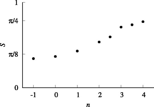
The characteristic size, S, increases with increasing [CO2], as shown in Fig. 3. A visual inspection of the ω₄₁ fields reveals that regions of subsidence and ascendance are finely intertwined in the control run, while they form two separated aggregated blobs for n = 4 (see Section S1 of the Supplemental Material for examples in particular time instants). According to Fig. 3 and further visual experience (not shown), aggregation develops gradually for increasing n with a transition-like point at $n\approx 2.$

Fig. 3. The temporal mean of the quantifier S of the characteristic size (see text) as a function of the logarithm n of the relative CO₂ concentration.

While convective self-aggregation is known to arise spontaneously (Wing et al., 2017), and its emergence when varying some parameter can be regarded as a transition to coarsening dynamics (Bray, 1994; Craig and Mack, 2013) in a spatiotemporally chaotic context (Mikhailov and Loskutov, 1996; Manneville, 2010), the origin of the temperature drops presented in Fig. 1 needs a partially independent explanation which we shall construct in the following sections.

3.3. Physical interpretation

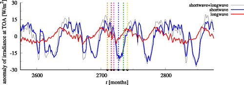
The temperature drops found in Fig. 1 are due to the appearance of low-level stratiform cloud fields. We illustrate this by comparing the globally averaged irradiance and its shortwave and longwave components at the top of the atmosphere (TOA), taking the n = 4 setup where the temperature drops are the most pronounced. Figure 4 shows that variations in the total irradiance are mostly determined by those in the shortwave flux, which exhibits a considerable deficit in the periods of the temperature drops (cf. Fig. 1). This means that the cooling is mainly due to more radiation being scattered back to space by clouds, without a discernible longwave effect with the same phasing. This implies that the relevant clouds are located at warmer temperatures, and hence in the lower troposphere.

Fig. 4. Globally averaged irradiance at TOA, as indicated in the legend, after subtracting the temporal mean, as a function of time. The time instants marked by vertical lines with black circles correspond to those of Figs. 6 and 7, and are also used later on. n = 4.

Figure 5 summarizes our hypothesized mechanism for the formation of the temperature drops at high CO₂ concentrations. Support shall be given in the following sections.

Fig. 5. Illustration of the cycle between ventilated and capped phases. A key factor for step 3) is the weak density gradient. Since density gradients are attenuated very fast (e.g. Sobel and Bretherton, 2000), the free tropospheric temperature profile of the convective region ($T^{\text{up}}$) is approximately imposed on the subsiding region. Below the free troposphere, the temperature profiles are different, which is illustrated by the difference between the black solid and gray dashed lines in the region of subsidence. These preconditions cause stability variations in the subsiding region that result in variations of the penetrative power of shallow convection. See the main text for more details (Section 4.1 for the labeled quantities).

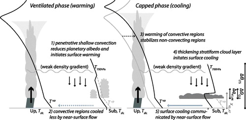
The domain of the simulation can be divided in an ascending and a subsiding part (‘Up’ and ‘Sub’ in Fig. 5). In the ascending part, deep convection occurs. In the subsiding part, penetrative shallow convection is present in the ground (or basic) state. Because the properties of the system depend on the state of the system, we think of the different states as phases, and this base state, in which shallow non-precipitating convection ventilates the thermal boundary layer of the subsiding region, thereby inhibiting the development of extensive stratiform cloud fields, is called the ‘ventilated phase’.

Deep precipitating convection couples the surface to the free troposphere in regions of large-scale ascent. In these regions the temperature roughly follows a saturated isentrope (moist adiabat) above cloud base, and because the amount of water that can be condensed increases with the cloud base temperature, this profile becomes steeper as the temperature at cloud base increases. In the absence of other processes gravity waves act to level the isopycnals, which effectively communicates this temperature profile also to non-convecting regions (e.g. Bretherton and Smolarkiewicz, 1989; Sobel and Bretherton, 2000), irrespective of (ocean) surface temperatures and near-surface air temperatures there, which are lower in our simulations.

There, in these non-convecting regions, non-precipitating shallow convection condenses water vapor in the lower part of the cloud layer and evaporates it aloft, helping maintain a cooler and moister ‘marine layer’ against warming by subsidence which still dominates the free troposphere (Riehl et al. (1951); Stevens (2007), and cf. Betts (1973) as well). The marine layer is separated from the air above the reach of the shallow convection by a layer of enhanced stability, something that on Earth is known as the marine or trade-inversion. When shallow convection is active enough to mix through this inversion, it can maintain the mass balance of the marine layer and in so doing efficiently mixes condensate up, and dry air down. This enhances surface evaporation, and inhibits the formation of stratiform cloud layers.

When the capping inversion becomes too strong, or the penetrative convection too weak, then the marine layer ceases to be ventilated, and stratiform clouds form beneath the inversion. These reduce the surface insolation and cause surface cooling. The surface cooling – which is confined to the capped marine layer – strengthens the contrast in the potential temperature between the surface (or near-surface) air and the lower mid-troposphere, strengthening the capping inversion and further inhibiting penetrative shallow convection. These effects thus constitute a self-amplifying local feedback. The termination of the penetrative nature of shallow convection in the subsiding region marks the beginning of what we shall thus call the ‘capped phase’, or a ‘cooling event’, as it is characterized by reduced surface insolation and cooling in the subsidence region.

Eventually the decrease in the ocean temperature in the subsiding region is communicated by the near-surface flow, which flows from cold to warm regions by virtue of pressure gradients, to the ascending region. The adaptation is not immediate but its time scale is determined by the heat capacity of the slab ocean (besides that of the transported air), a fact we established by performing additional simulations with different surface heat capacities (equivalent slab ocean depths), and for which the time scale varied accordingly (similarly as found by Coppin and Bony, 2017).

Deep convection quickly communicates surface temperature changes in the ascending region vertically throughout the troposphere, and these are communicated horizontally by gravity waves, thus reducing the temperature in the free troposphere also in the subsiding region. The cooling proceeds until shallow convection can re-establish itself, thereby desiccating the low-level stratiform clouds. From this point on, the beginning of the ventilated phase, the decreased degree of cloudiness leads to increased surface insolation, the slab ocean starts warming, and the cycle begins anew.

For this process to be effective, two conditions must be met: the areas of cooling must be coherent and large-scale, and the difference between the lapse rate in the regions of precipitating deep convection and those of non-precipitating shallow convection must grow sufficiently large in the course of time to finally inhibit the ability of the latter to maintain a deep mixing layer. These conditions appear to explain differences in behavior between simulations with low and high [CO₂], even if the reason for greater coherence at high n remains unclear.

The dynamics adumbrated above are discussed in greater depth in the following sections. In the next section we analyze the n = 4 case, for which the cycling between ventilated and capped phases of the system is prominent and shows some degree of regularity. Thereafter, in Section 5, we address the differences between runs with different [CO₂]. The purpose of these sections is to justify the mechanisms articulated above, the conclusions discussed in Section 6 are thus comprehensible without reading the next two sections.

4. Dynamic analysis of n = 4 cooling events

4.1. Temporal evolution

Figure 6 shows the emergence and desiccation of the low-level stratiform cloud field in association with one full cooling event. Snapshots in time, with global patterns of different character, are presented (cf. Fig. 4). The location of the low-level stratiform clouds is evident in patterns and magnitude of reflected shortwave radiation. Deep convection is indicated by the occurrence of precipitation in the region of ascendance (${\omega }_{41}<0$).

Fig. 6. Snapshots of upward shortwave irradiance at TOA. The time instants are indicated in the panels and are also marked in Fig. 4. Cyan contour lines denote precipitation in $5\text{mm}/\mathrm{d}$ intervals, solid green lines outline the boundary of the dry-subsiding region (ω₄₁ > 0 with $q<\frac{2}{3}{\text{max}}_{\text{spatial}}(q)$ at level 41, see also the main text), and green dashed lines demarcate the boundary of the region where ω₄₁ > 0. n = 4.

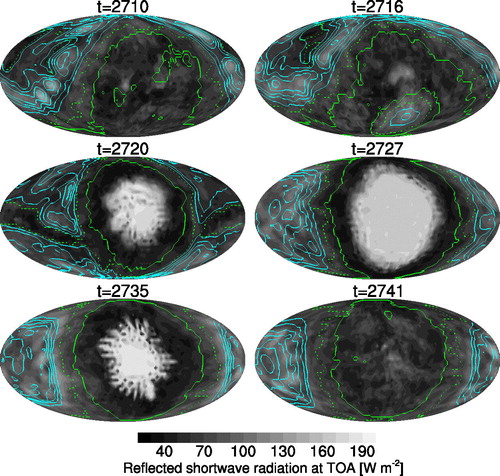
The highly reflective stratiform clouds show up for a period of about 15 months, between t = 2720 and t = 2735, in the region of subsidence as defined by ω₄₁ > 0. However, the subsiding region extends beyond the region where the stratiform clouds form. For example, at t = 2720, a narrow channel of subsidence forms a belt around the globe. To capture these differences and to better identify the region that is relevant for the temperature drops in addition to ω₄₁ > 0, a second condition, measuring the dryness of the lower free troposphere, is formulated. This second condition is expressed as a condition on the specific humidity q at level 41: $q<\frac{2}{3}{\text{max}}_{\text{spatial}}(q).$ Figure 6 demonstrates that the region defined by these two conditions, which we shall call the ‘dry-subsiding region’, matches well with the region containing the low-level cloud field. The existence of this smaller region within that of subsidence, and its approximate empirical matching with our dry-subsiding region, is demonstrated further in Section S2 of the Supplemental Material.

By t = 2727, the stratiform cloud field is well developed, before it begins to dissipate (see t = 2735), with areas of penetrative shallow convection desiccating the stratiform cloud field in between what look like cloud streets.

The vertical structure of the lower troposphere at the different points in time clarifies the changes that occur in the course of a cooling event. Figure 7 presents selected profiles averaged over the dry-subsiding region during the same event as in Fig 6. Between t = 2720 and t = 2735, when the low-level stratiform cloud field is well established, the cloud liquid water content X associated with the stratiform clouds is located between 850 hPa and 950 hPa, at model levels 42 to 44. This cloud field is capped by a layer of enhanced stability, as can be seen from the vertical profile of the potential temperature θ. As a measure of this stability, we introduce the symbol Δθ_CLS to denote the difference in θ between levels 41 (≈ 820 hPa) and 44 (≈ 943 hPa), and call it the ‘cloud-layer stability’. This is a vertically localized measure of the strength of the inversion separating the moist near-surface layer from the free troposphere.

Fig. 7. Vertical profiles of the potential temperature θ, the specific humidity q, and the cloud liquid water content X, averaged for the dry-subsiding region, at the time instants of Fig. 6 (also marked in Fig. 4) as indicated in the legend. The labeling refers to the sectioning introduced in Fig. 10; sections A and E compose the ventilated phase. Model levels are marked on one vertical axis at the corresponding pressure coordinate averaged spatially (over the dry-subsiding region) and temporally. n = 4.

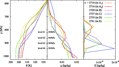
At and above level 41, θ increases less markedly with height and approaches a value more consistent with a moist adiabat, 5 K km⁻¹. For this reason, and because the stratiform cloud layers form below this level (see X), we take this level to be lowest one unambiguously located in the lower free troposphere, so that the vertical pressure velocity ω at this point is indicative of the strength of the mean divergence of the low-level flow. This motivates our choice of ω₄₁, ω at level 41, as one of our chosen indicators of the ‘dry-subsiding’ region.

Figure 7 further demonstrates that moisture, as indicated by the profile of the specific humidity q, is confined to lower levels (42 and below) at these time instants, which implies the absence of penetrative shallow convection acting to mix moisture away from the surface. However, moisture is effectively transported by convection to higher levels (up to 40 and 41) at the other three time instants (t = 2710, 2716, and 2741), which is in harmony with the presence of clouds from level 41 upwards (see the cloud liquid water content X), and with the absence of a layer of strong stability (see the potential temperature θ; note that this does not exclude the presence of relatively stabler layers throughout the vertical range of the shallow convection). We shall use the difference $\Delta q_{41,44}$ in the specific humidity between levels 41 and 44 as a proxy for the strength of the shallow convection. In the n = 4 simulation, it empirically appears that penetrative shallow convection is off or absent (capped) and on (ventilating) when $\Delta q_{41,44}<-0.005$ and $\Delta q_{41,44}>-0.005,$ respectively, corresponding to the two phases introduced earlier.

While stratiform clouds at the inversion layer are supposed to be most closely related to the vertically localized stability measure Δθ_CLS, the strength of the shallow convection should rather be set by stability properties on larger vertical scales. For investigating this aspect of shallow convection, we utilize the traditional lower tropospheric stability (LTS, Δθ between 700 hPa and the surface, Δθ_LTS; Klein and Hartmann, 1993). While this is usually linked to the presence or absence of low-level stratiform clouds in the literature (e.g. Klein and Hartmann, 1993), it shall be shown to play a somewhat different role in the dynamics of our present model.

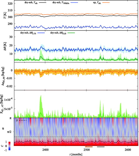
Figure 8 shows the details of the time evolution of the quantities most relevant for the cooling phenomenon, which are summarized in Table 2. All quantities, except for the surface temperature in the ascending region and the spatial autocorrelation function, are indicative of values in the dry-subsiding region. In addition to the mean, the shading of a variable denotes the limits (5th and 95th percentile) of its distribution over the dry-subsiding region. The shading emphasizes the considerable variability, and reminds us that this is a dynamic system with many degrees of freedom.

Fig. 8. The time evolution of several quantities as given on the vertical axis and in the legend; see Table 2. Solid lines mark spatial means, while shaded areas correspond to the interval between the 5th and the 95th spatial percentile. In the uppermost plot, the corresponding spatial region is indicated in the legend; plots below concern the dry-subsiding region. The bottom plot shows the spatial autocorrelation function of ω₄₁ color coded, separately for each time step t, as a function of the angle α of separation. The dashed black line, S, is a measure of size (see Equation (2)(2) $$S={\int }_0^{\alpha (C=0)}C(\alpha )\mathrm{d}\alpha .$$(2) and the corresponding explanation), and it is compared to an ideal value (dot-dashed black line) that would correspond to a cosine-shaped autocorrelation function. The vertical lines with circles mark the time instants selected for Figs. 6 and 7, and they also appear, together with the vertical lines with triangles, in Figs. 10–11. The black and orange line segments next to the horizontal axis correspond to time intervals with a major and a minor cooling event, and are highlighted in Figs. 10–11. n = 4.

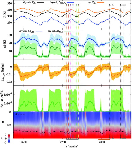
Table 2. The quantities most relevant for the cooling dynamics.

Notation	Definition	Comment
Tsfc	Surface temperature
$T_{700\text{hPa}}$	Temperature at 700 hPa
ΔθCLS	Cloud-layer stability: difference of potential temperature between model levels 41 and 44	Vertically localized inversion strength
ΔθLTS	Lower tropospheric stability: difference of potential temperature between 700 hPa and the surface	Stability vertically encompassing the lower troposphere
$\Delta q_{41,44}$	Difference of specific humidity between model levels 41 and 44	Proxy for the strength of shallow convection
$X_{42\dots 47}$	Cloud liquid water content averaged from model level 42 to model level 47	Amount of low-level stratiform clouds
C(α)	Spatial autocorrelation function of the ω41 field; see Section 3.2	Isotropic quantifier of spatial similarity; a function of the angular separation α
S	See Equation (2)(2) $$S={\int }_0^{\alpha (C=0)}C(\alpha )\mathrm{d}\alpha .$$(2)	Characteristic size of spatial structures

In the ventilated phase, when the surface temperature in the dry-subsiding region (‘dry-sub’, T_sfc) increases, there are practically no low-level clouds (see the cloud liquid water content averaged for levels 42–47, denoted by $X_{42\dots 47}$), the cloud-layer stability Δθ_CLS (between levels 41 and 44) stays at a small constant value, and penetrative shallow convection increasingly mixes moisture to upper levels, as the growing difference $\Delta q_{41,44}$ in the specific humidity indicates. The traditional lower tropospheric stability, Δθ_LTS, is more variable than most other quantities of the figure. Its phasing depends on the 700 hPa temperature of the dry-subsiding region (‘dry-sub’, $T_{700\text{hPa}}$), which is practically in phase with the surface temperature in the ascending region (‘up’, T_sfc), as expected from convection in the latter region setting the thermal structure of the free troposphere. With this phasing, Δθ_LTS does not drop to its minimal value immediately at the beginning of the ventilated phase, but with a certain lag, and starts increasing only thereafter. This time evolution is most evident in the long ventilated phase around t = 2800.

The beginning of the decrease in the dry-subsiding surface temperature (e.g. at t = 2717, after the second vertical line) coincides with a sharp increase in $X_{42\dots 47}$ and Δθ_CLS, and a similarly sharp decrease in $\Delta q_{41,44}.$ $\Delta {\theta }_{\text{LTS}}$ also increases, but more slowly than Δθ_CLS. After a considerably delayed maximum in Δθ_LTS (with respect to Δθ_CLS), and a coinciding minimum in $\Delta q_{41,44}$ (e.g. between t = 2720 and t = 2727, the third and the fourth vertical lines), Δθ_LTS and $\Delta q_{41,44}$ begin to decrease and increase, respectively. This change can possibly be interpreted as a recovery of the penetrative shallow convection. A more detailed analysis of the relationship between Δθ_LTS and $\Delta q_{41,44},$ based on their spatial variation, is given in Section S3 of the Supplemental Material, and indicates that $\Delta q_{41,44}$ becomes larger in the middle of the dry-subsiding region after the formation of the stratiform cloud field than at the edge of the dry-subsiding region and at the beginning of the cooling event. A gradual global increase in $\Delta q_{41,44}$ can nevertheless also be observed.

Irrespective of the precise interpretation of the gradual increase in $\Delta q_{41,44}$, this quantity suddenly jumps up at some point, as seen in Fig. 8 for example between t = 2735 and t = 2741 (the last two vertical lines with circles), which indicates that penetrative shallow convection is becoming effective in ventilating the dry-subsiding region. At this point, the low-level clouds desiccate, and the dry-subsiding surface temperature can start increasing again.

The characteristic size S of the spatial structures in the ω₄₁ field, and its spatial auto-correlation function C(α), can also vary with the phase of the cycle between a ventilated and a capped subsidence region, but variation does not occur at each cooling event. In particular, Fig. 8 shows that C(α) exhibits a bipolar structure with S being close to a theoretical maximum (see Section 3.2) most of the time. However, at the beginning of certain (but not all) cooling events, smaller spatial structures are introduced, with a positive correlation between ω₄₁ on two opposite sides of the sphere (C > 0 for $\alpha =\pi$) (a good example is the substantial cooling event ending before the orange line segment in Fig. 8, and a counterexample is the one starting after the orange line segment, at the first triangle-labeled vertical line).

The introduction of smaller spatial scales is related to the formation of a new ascending region at a location where subsidence was present earlier, as illustrated by snapshots of shortwave irradiance and precipitation fields in Section S4 of the Supplemental Material. We hypothesize that the formation of a new convective area triggers the shutdown of penetrative shallow convection in its neighborhood through a local additional increase in stability, which is anyway increasing globally. Such a spatial rearrangement is not observable if sufficient time elapses after the end of the last cooling event, so that it is not an essential ingredient for the main processes that we are studying.

It is here that we should mention the presence of cooling events of much smaller amplitude and duration (‘minor events’), like the one near t = 2800 (before the middle of the orange line segment in Fig. 8). They usually appear after the major events, and are always characterized by smaller spatial structures. In this sense, they seem to be relatives of the minor fluctuations that form a temporally continuous background for any low CO₂ concentration.

To illustrate these minor fluctuations and to provide a contrast to the n = 4 case, we show the counterpart of Fig. 8 for n = 1 as Fig. 9. We can see that these minor fluctuations are actually governed by similar processes as those described for the major cooling events, but the scales are much smaller, both in terms of the amplitude and the duration, and also in terms of the size of the spatial structures present, corresponding to an intertwined structure between ascendance and subsidence. Events with somewhat larger scale happen e.g. near t = 2390 and t = 3530 (the latter highlighted by a black line segment). Although they are still much smaller than the major events for n = 4, these somewhat larger events obey different statistics compared to the minor fluctuations, as the skewness discussed in Section 3.1 indicates.

Fig. 9. Same as Fig. 8 for n = 1.

4.2. Phase space analysis

Now let us return to the analysis of the major cooling events for n = 4, where we adopt a phase space perspective. For this purpose the processes described in relation with Fig. 8 are represented by direct relationships among the monthly-mean values, thereby defining projections of the phase space, Fig. 10. The phase space representations identify five main different sections (from A to E; section A has two subsections, but they are the same in all main tendencies). Sections A and E compose the phase when shallow convection is effective at ventilating the lower troposphere, section C can be identified with the capped phase, and sections B and D represent transitions between these two main phases. The time instants considered in Figs. 6 and 7, marked by circles, are characteristic to these sections (there are two instants for section A, in its two subsections), and points separating the consecutive sections during a particular cooling event are also marked (by triangles) both in Figs. 8 and 10.

Fig. 10. Phase space projections for quantities in the dry-subsiding region: the spatial mean of the surface temperature T_sfc, of (a) the cloud-layer stability Δθ_CLS and (b) the lower tropospheric stability Δθ_LTS, and of the cloud liquid water content $X_{42\dots 47}.$ All months of the simulation are plotted between t = 2000 and 5000 (to optimize visibility), and consecutive months are linked by a colored line. The labeled arrows indicate the direction of the time evolution, and correspond to separate sections in the dynamics (see text). The time instants marked by circles and filled triangles in Fig. 8 are also marked here in black, with the same symbols. In panel (b), an unfilled triangle is also displayed between the two subsections of section A, corresponding to t = 2809 along the orange trajectory. The time evolution highlighted in black (between the first and the last circle) and in orange (before the first triangle) corresponds to a major and a minor cooling event, respectively (see also in Fig. 8). n = 4.

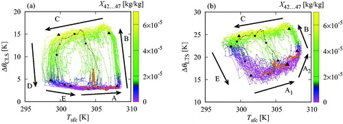
The cloud-layer stability, Δθ_CLS, correlates strongly with the cloud liquid water content, $X_{42\dots 47}$, which is evident in Fig. 10a. Both quantities co-vary strongly in the transition phases (B and D), and both are approximately constant in the other phases (A, E and C), i.e., during the bulk of the two main phases. This is in harmony with our picture whereby phases in which shallow convection ventilates the lower troposphere are characterized by an absence of low-level stratiform clouds (A and E), and in the phase in which shallow convection is capped, low-level stratiform clouds predominate (C). It is in these phases, of relative stationarity in Δθ_CLS and $X_{42\dots 47}$, when most of the warming (E–A) and cooling (C) happens, as indicated by the surface temperature T_sfc in Fig. 10a.

Δθ_CLS and thus the presence of stratiform clouds is strongly related to the strength of the penetrative shallow convection, characterized by our proxy $\Delta q_{41,44}$. This is illustrated in Section S5 of the Supplemental Material, in which the transition phases of $\Delta q_{41,44}$ are also identified as sections B and D. At variation with Δθ_CLS, Δθ_LTS is already increasing in section A (see Fig. 10b), and we hypothesize that this process is what leads to the attenuation of shallow convection, finally preventing it from penetrating the layer where stratiform clouds form then (see again Section S5 of the Supplemental Material for a direct comparison of the tendencies of Δθ_LTS and $\Delta q_{41,44}$).

In the bulk of section A, labeled as A₁ in Fig. 10b, Δθ_LTS is increasing at a moderate rate compared to a separate subphase at the end of section A, labeled as A₂, where Δθ_LTS increases rapidly. The latter already results from the reduced penetrative power of the shallow convection, which leads to the lack of two cooling effects in the lower mid-troposphere but does not yet induce stratiform cloud formation: note that $X_{42\dots 47}$ is still low and T_sfc is still increasing in section A₂. Cooling at 700 hPa was earlier provided by evaporation and a strong moisture gradient at the top of the shallow convection, but these effects discontinue as shallow convection does not reach as high as before (as indicated by the dropping humidity around 700 hPa observable in the vertical profiles of q and X at t = 2716 in Fig. 7). Of course, the rapid increase of Δθ_LTS in section A₂ is an important local feedback anticipating the shutdown of ventilative shallow convection, but the original reduction of the penetrative power, ending up in the transition to section A₂, is thought to have a nonlocal origin.

In particular, the underlying mechanism we propose relies on the moist adiabat in the deeply convecting region. This moist adiabat is what sets the temperature profile globally, and as the surface is warming in section A, the slope of this adiabat becomes steeper (e.g. Fig. 5b in Bony et al., 2016). This steeper profile imposed on the subsiding region may be seen as stronger stability there, becoming more difficult to overcome by shallow convection without precipitation. This is supposed to be the case even though surface temperature is increasing in the subsiding region, too, allowing penetrative functioning under increasingly high stability. The effective stability is further amplified here in so far as the absence of deep convection leads to a drier free troposphere, which increases radiative cooling in the lower troposphere, further stabilizing it with respect to the free troposphere. In Section S6 of the Supplemental Material, we document how differences in the virtual potential temperature at 700 hPa between the regions of ascendance and subsidence develop to further articulate these dynamics.

Based on the ideas presented so far, especially on the dependence of the slope of the moist adiabat on surface temperature, we can formulate now a simplified but illustrative condition for the capping of shallow convection and the corresponding initiation of a cooling event: the difference in the surface temperature between the ascending and the subsiding regions has to be sufficiently large. But note that what counts as “sufficient” depends on the actual surface temperature of the subsiding region.

The explanation for the restart of penetration by shallow convection is supposed to be similar to that for capping. According to Fig. 10b, Δθ_LTS is decreasing in section C, the capped phase, and this decrease in stability sooner or later allows penetration again just as penetration was allowed before the cooling event. The reason for the decrease in stability is that surface cooling in the dry-subsiding region is followed by surface cooling in the ascending region, too (but with a lag of about 8 months, which is important for giving time for the cooling event to develop), and this surface cooling is amplified in the free troposphere by virtue of the moist adiabat when it is communicated to the free troposphere by deep convection.

With these dynamics in mind it is helpful to review the nature of minor cooling events. In Fig. 10, the path of such an event (cf. Fig. 8) is highlighted in orange. During this event the state of the atmosphere in the dry-subsiding region does not go around the entire cycle; rather the cooling event appears as an aborted short-circuit of the cycle. Because minor events are always associated with the appearance of new convective blobs within the dry-subsiding region (see C(α) in Fig. 8), it emphasizes the importance of the spatial coherence required to realize a major cooling event. This suggests that the dynamics of the major cooling events likely explain global temperature fluctuations even at small values of n, but the lack of spatial organization at these values of [CO₂] prevents the events from establishing themselves on a global spatial scale.

The nature of major events is refined by noting that the second circle in Fig. 10b (referring to t = 2716) is not where we marked section A₂ in this figure. This emphasizes that, beyond minor events, also major events can begin at basically any point in section A, there is no strict threshold e.g. in Δθ_LTS or T_sfc that would open the opportunity for the formation of a cooling event of arbitrary size. (This is so in spite of the observation that section A₂ usually appears less sharply for lower T_sfc.) The absence of a threshold raises again the question about the difference between runs with different CO₂ concentration.

5. Runs with different CO₂ concentration and the role of spatial organization

It is clear already from Fig. 1 that both the amplitude and the duration of the cooling events grow with increasing CO₂ concentration (i.e., with increasing n). A more complete comparison is given in Fig. 11 in a representation similar to that of Fig. 10b. Here the lower tropospheric stability is constructed with a reference level of 950 hPa: assuming a cloud base at the top of the well-mixed sub-cloud layer at 950 hPa (implying the potential temperature to be practically the same here as on the surface), this choice facilitates a comparison with the value that the lower tropospheric stability would adopt if the stratification were set by the moist adiabat calculated with the same assumption (Bony et al., 2016). We emphasize that this adiabat puts a lower limit on the stratification: if stability is stronger than this, convection is certainly impossible. In fact, in the subsiding region shallow non-precipitating moist convection follows an adiabat closer to the dry adiabat, and the clear dry air above the shallow convecting layer ensures that radiative cooling is concentrated in the marine layer. With these caveats the indication of the adiabat is intended to serve more as a guide.

Fig. 11. Phase space projection: the spatial mean of the near-surface potential temperature θ_950hPa, the lower tropospheric stability Δθ${}_{\text{LTS}\left(950\text{hPa}\right)}$, and the cloud liquid water content $X_{42\dots 47}$ in the dry-subsiding region. Additional features are marked as in Fig. 10b. Furthermore, Δθ${}_{\text{LTS}(950\text{hPa})}$ implied by the moist adiabat at given θ_950hPa (Bony et al., 2016) is indicated as a black line. Note that the actual stratification is not set by this adiabat, see the main text for more detail. The different panels concern setups with different CO₂ concentration, as indicated.

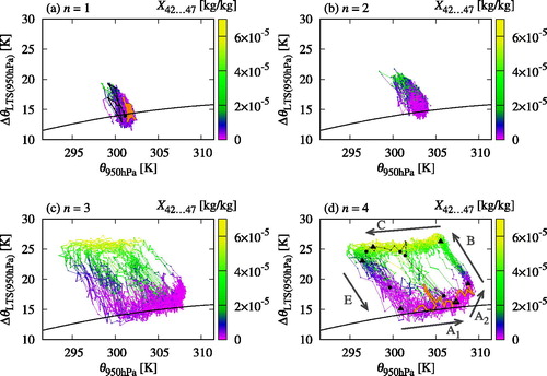
Figure 11 shows that higher near-surface (potential) temperatures are typically reached for higher CO₂ concentration before a cooling event occurs, and that these temperatures are accompanied by higher values of the lower tropospheric stability. As discussed earlier, stratification in the subsiding region is determined by the moist adiabat in the ascending region, and a cooling event begins when this stratification becomes too stable for local shallow convection to maintain its state. A warmer ascending region and a corresponding steeper moist adiabat might thus actually unfavor reaching higher temperatures globally. However, shallow convection in the subsiding region also becomes more “tolerant” against stability if the surface is warmer, i.e., it functions properly at a steeper lapse rate, as the black lines in Fig. 11 approximately indicate (with the mentioned caveats). When penetration shuts down is determined by these two aspects of our setup’s convective processes, and it would be difficult to argue for the increasing temperature of the typical shutdown point. Changes in the “tolerance” of non-precipitating shallow convection and thus in the exact shutdown point will also depend on the details of how shallow convection is parameterized in the model, but the gist of this behavior is not model dependent as it lies at the origin of explanations of the stratocumulus to cumulus transition on Earth (Bretherton and Wyant, 1997).

Nevertheless, Fig. 11 also makes clear that the tendency of reaching higher surface temperatures (further to the right in the plots) cannot serve as an exclusive explanation for the larger amplitude of major cooling events. As n increases, the cycle expands to the top and to the left as well, even for trajectories that do not extend further to the right (remember from Section 4.2 that even major events can begin at basically any near-surface temperature, as also illustrated clearly by the black trajectory segment in Fig. 11d).

A natural candidate that could underlie the inflation of the cycle could be an increased lag beween the regions of subsidence and ascendance. This lag is essential for the delayed decrease of Δθ_LTS and is thus one of the basic factors determining the duration of the cooling events. Its value is mainly set by the heat capacity of the mixed-layer ocean in the ascending region and that of the near-surface air transported from the subsiding to the ascending region. While the former is not expected to vary much between different runs when regarding the ascending region as a whole, the latter may be subject to some variation. Computing lagged correlations between the surface temperatures spatially averaged for the whole ascending and dry-subsiding regions indicates lags between 5 and 9 months. In particular, a value of 6 months is found for n = 1 and 2 and 8 months for almost all n > 2. This increase in the lag, while certainly playing some role, does not seem to fully explain the variation in the size of the cycle for different CO₂ concentrations and requires its own explanation as well.

Further insight into the cooling dynamics may be obtained from minor cooling events, highlighted in orange in Figs. 11a and d. The graphs confirm that they do not visit the entire cycle, whereby their path is plotted in terms of the phase space of the state of the dry-subsiding region as a whole. The same is true for the somewhat larger event in Fig. 11a, for n = 1 (highlighted in black, see the black line segment next to the horizontal axis in Fig. 9). This is consistent with the shutdown of penetrative shallow convection taking place only in some part of the dry-subsiding region, which would not be surprising given that spatial organization is much weaker for n = 1 than for n = 4 (see Fig. 3). In particular, the subsiding and the ascending regions have very complicated and intertwined shapes with several “bottlenecks” for n = 1 (see Section S1 of the Supplemental Material for an example), preventing the propagation of effects through the whole regions. Similar dynamics are also evident in other models, and appear to explain both temperature fluctuations at low n (Coppin and Bony, 2017), and the tendency of spatially varying temperatures to support more low clouds (Coppin and Bony, 2018).

The picture that develops is that synchrony is what makes a distinction between major and minor events, or, to be more precise, the size of any event depends on the the degree of synchronization. This is in harmony with the experience, from Fig. 2, that the probability density of the global mean surface temperature is Gaussian distributed when dominantly minor events are present (for lower CO₂ concentrations), but Gaussianity is distorted when more and more major events occur. In the former case, the addition of the temperature from different small-area patches (for calculating the global mean), in which similar processes take place but with uncorrelated phases, may result in a Gaussian distribution according to the central limit theorem. Meanwhile, coherency lets the single events’ characteristics be observed in the probability density of the global mean, and these characteristics are expected to be non-Gaussian due to the very specific shape of the time evolution of the surface temperature during a single event.

We recall from Section 3.2 that higher CO₂ concentrations are accompanied by enhanced spatial organization in our model setup, starting from a rather disorganized pattern for n = 0 or 1, until, based on spatial autocorrelation, almost perfect aggregation for n = 4. As explained, self-aggregation at near-global scales might well be what provides with the possibility of synchronization. Both synchrony and larger spatial scales are true candidates for explaining the larger amplitude and the longer duration of the events.

In particular, a key factor might lie in the organization of the deeply convecting region. If a high temperature anomaly under deep convection only appears in a small patch as a result of local fluctuations, it will, on the one hand, facilitate the shutdown of shallow convection in nearby areas of subsidence only, and, on the other hand, will be easier and faster (e.g. in terms of the above-mentioned lag) to cool back to support a moist adiabat imposing a stability compatible with penetrative shallow convection in the surroundings. Meanwhile, the region of subsidence works differently: once stratiform clouds appear in some part of it, effects from outside this area cannot warm back its surface due to the isolating inversion and to the outward-directed near-surface flow, irrespective of the spatial organization.

While the latter thoughts explain why cooling events finish less easily and thus last longer in a well-organized spatial configuration, it is also interesting to consider how initiation is affected by spatial organization. Cooling events are basically triggered by a sufficiently high temperature difference between an area of subsidence and its deeply convecting surroundings, cf. Section 4.2. Higher temperature differences are supposed to be reached more easily if the two kinds of regions are separated and self-aggregated. Moreover, feedbacks that help maintain an aggregated state by increasingly suppressing convection in areas of subsidence under an increasingly aggregated global picture (e.g. an increasing contrast in moist static energy as discussed by Wing and Emanuel, 2014) may also facilitate the capping of shallow convection.

These factors might contribute to explaining why a large-scale cooling event appears right after each recovery from the previous event for n = 4, as opposed to the erratic inter-event distribution for n < 4. For small n, the continuous background appearing to be governed by the same dynamics as those of individual cooling events (e.g. in Fig. 9) is explainable by the diversity of a very incoherent spatial organization in which a “cooling event” always appears somewhere. Note that such a background of very minor “events” is completely missing for large n (e.g. in Fig. 8, and such cooling dynamcs are also completely absent for n = 3 in longer ventilated periods). As a result, high-frequency variability has a much smaller amplitude for large n than for small n (compare e.g. the time evolution between t = 2700 and 2800 for n = 3 and n = 0 in Fig. 1).

In spite of all the above, the causal relationship between spatial organization and major events is not obvious if well-defined at all. In particular, we have not addressed so far why spatial organization is enhanced at higher CO₂ concentration in our model. Spatial self-organization, or, more precisely, convective self-aggregation, is a topic on which there is a wide and growing literature (Wing et al., 2017). Craig and Mack (2013) already pointed out its relationship to coarsening (Bray, 1994), and positioning this aspect of the phenomenon in the context of spatiotemporal chaos (Mikhailov and Loskutov, 1996; Manneville, 2010) may shed more light on its parameter dependence. Further studies may possibly be carried out within the RCEMIP project, which aims at obtaining a better understanding of convective self-aggregation across models (Wing et al., 2018).

6. Conclusions

Simulations with a comprehensive climate model, run in conditions of radiative-convective equilibrium at varying concentrations of atmospheric CO₂ and coupled to a slab ocean, evince both reassuring and surprising dynamics. The dynamics are reassuring in that the non-monotonicity of the apparent feedbacks noted in previous studies performed with uniform and fixed sea-surface temperatures (Becker et al., 2017) does not seem to be realized when the atmosphere is coupled to a slab ocean and explored as a function of increasing CO₂ concentration. This finding, that feedbacks are different and fundamentally well-behaved when the system is coupled to dynamically varying sea-surface temperatures, echos the finding of a related study by Coppin and Bony (2018).

The dynamics are disconcerting in terms of the magnitude of low-frequency variations (with time scales of the order of 10 to 100 months) in globally averaged surface temperatures, particularly for large increases in atmospheric CO2 concentration, with a factor of 8-16 relative to pre-industrial values. The magnitude of these temperature variations is around 10 K in the global spatial mean. Although the long-term (climatological) mean properties of the equilibrium response vary smoothly as a function of the CO₂ concentration, a change in the nature of variability introduces strong nonlinearity in the response at high concentrations. In particular, the climatological mean value of the global mean surface temperature practically stops responding to an increase in the CO₂ concentration. This practically zero climate sensitivity suggests that the effect of a feedback on the global mean surface temperature may turn out to be as strong as the radiative effect of CO₂, even if the feedback varies smoothly and monotonically and is well-behaved in general. This may be regarded as a warning that even “first estimates” of Earth’s climate sensitivity may be inaccessible without taking into account feedbacks: there is no theoretical argument for treating them separately from the radiative effect of CO₂ as second-order corrections.

In our model system, the mechanism that counteracts the radiative effect of CO₂ – in the long-term temporal mean – is the emergence of global-scale cooling events caused by extended stratiform cloud fields. Although causalities are not demonstrated in a strict sense, the line of our argumentation is highly plausible and can be summarized as follows: Higher temperatures result in a steeper moist adiabat in the region of ascendance, imposing higher stability on the subsiding region. A sufficiently high temperature contrast between the two regions can result in the shutdown of penetrative shallow convection in the latter. If this happens, cooling of the lower mid-troposphere due to shallow convection stops in this region, and the capping of the shallow convection leads to a build-up of moisture and low-level stratiform clouds, which cool the ocean surface. At the beginning, these effects further increase the stability, which is thus a self-amplifying feedback. The decrease in the surface temperature is communicated by the near-surface flow to the ocean surface in the ascending region with a considerable delay. From there, deep convection quickly communicates temperature changes throughout the global free troposphere. This cooling process, enhanced in the mid-troposphere by the deep convection, reduces the stability in the subsidence region, allowing penetrative shallow convection to re-establish itself, causing the desiccation of the low-level stratiform clouds. A reduction in low-level cloudiness leads then to increased surface insolation, and the ocean starts warming: the cycle starts from this ‘ventilated phase’ once more, with a certain degree of irregularity as to be expected given the chaotic nature of the system.

The conclusion about the role that penetrative shallow convection plays in preventing the formation of low-level stratiform clouds is supported by simulations (mentioned in Section 1) in which parameterized convection was turned off. Surface temperatures in these simulations are much lower and near-surface cloudiness is much higher, consistent with the complete absence of penetrative shallow convection (Stevens et al., 2019).

While the effectiveness of shallow convection in ventilating the lower troposphere is mostly determined by the stability, the absence of a clear threshold in stability for event formation (even in a particular simulation) reminds us that the system is dynamic and complex. Many factors, some of which undoubtedly will be model dependent, influence whether or not penetrative shallow convection gives way to more stratiform cloudiness, thus enriching the trajectories in low-dimensional phase space projections such as those that we have examined.

In fact, the kind of dynamics described above is observable for any CO₂ concentration: for concentrations around the pre-industrial one, it actually appears to dominate temporal variability by providing a small-amplitude but continuous background. While the details likely depend on the physical parameterizations used in our study, similar dynamics are also observed in other models (Coppin and Bony, 2017, 2018), even if these studies have not explored such extreme warming scenarios as ours. In our simulations, the main difference between low and high CO₂ concentrations is that higher atmospheric stability, shutting off penetrative shallow convection in the subsidence region, is only widespread and spatially coherent at high concentrations. This is hypothesized to be related to the emergence of larger, more coherent spatial structures, i.e., to convective self-aggregation.

The importance of large-scale coherence for realizing major cooling events that dramatically influence global temperatures suggests that these effects are very likely to be exaggerated by the idealized nature of the simulations performed here. On Earth such large-scale coherence would be inhibited by externally imposed inhomogeneities, ranging from top-of-atmosphere insolation gradients and their seasonality to surface heterogeneities (continents) and to instabilities in the dynamic ocean and the atmosphere arising from spatial temperature gradients in the presence of rotation. In particular, global-scale atmospheric and oceanic circulations shaped by planetary waves are expected to dominate large-scale spatial patterns of convection as opposed to self-organization by aggregation.

However, the dynamics we see in our idealized configuration may color the larger-scale circulations, for instance by strengthening air-sea interactions, like in El Niño which shares aspects of these dynamics (e.g. Dommenget, 2010; Rädel et al., 2016). In fact, the physics underpinning these dynamics is apparent in the broader tropics of our Earth and in many models as well, and this highlights the uncertainty as to potential changes in tropical circulations as climate warms, beyond the uncertainty about the role of such variability in the dynamics of the present-day tropics. By idealized investigations, we may isolate these physics which in the present world might be confined to smaller subsystems or might not even be expressed on their own, but certainly make part of the interplay between the cold and warm tropical oceans. In particular, there is some evidence that the El Niño (and likewise the Pacific Decadal Oscillation) reflects a response to Atlantic warming (Ham et al., 2013; Luo et al., 2017) in ways that are reminiscent of what we see in our model. Therefore, our study indicates that tackling the mentioned uncertainties requires advances in understanding factors controlling the depth of penetrative shallow convection and its ability to ventilate the marine boundary layer in trade-wind regimes, where surface temperatures are relatively low and regimes of shallow clouds prevail.

Supplementary data

Supplemental data for this article can be accessed here.

Disclosure statement

No potential conflict of interest was reported by the authors.

Correction Statement

This article has been republished with minor changes. These changes do not impact the academic content of the article.

Additional information

Funding

This research was supported by the Max-Planck-Gesellschaft (MPG), and computational resources were made available by Deutsches Klimarechenzentrum (DKRZ). Primary data are maintained and made available by the Max Planck Institute for Meteorology and can be accessed by contacting [email protected]. The authors thank the internal reviewer Jessica Vial and two anonymous reviewers for some very helpful comments. GD was supported by the European Social Fund under CAIB grant PD/020/2018 "Margalida Comas". TM received funding from the European Research Council (ERC) Consolidator Grant 770765.

References

- Arnold, N. P. and Randall, D. A. 2015. Global-scale convective aggregation: Implications for the Madden-Julian Oscillation. J. Adv. Model. Earth Syst. 7, 1499–1518. Oct. doi:10.1002/2015MS000498
- Becker, T. and Stevens, B. 2014. Climate and climate sensitivity to changing CO2 on an idealized land planet. J. Adv. Model. Earth Syst. 6, 1205–1223. Dec. doi:10.1002/2014MS000369
- Becker, T., Stevens, B. and Hohenegger, C. 2017. Imprint of the convective parameterization and sea-surface temperature on large-scale convective self-aggregation. J. Adv. Model. Earth Syst. 9, 1488–1505. doi:10.1002/2016MS000865
- Betts, A. K. 1973. Non-precipitating cumulus convection and its parameterization. Quart J. Royal Met. Soc. 99, 178–196. doi:10.1002/qj.49709941915
- Bony, S. and Dufresne, J.-L. 2005. Marine boundary layer clouds at the heart of tropical cloud feedback uncertainties in climate models. Geophys. Res. Lett 32, 2055.
- Bony, S., Stevens, B., Coppin, D., Becker, T., Reed, K. A. and co-authors. 2016. Thermodynamic control of anvil cloud amount. Proc. Natl. Acad. Sci. USA. 113, 8927–8932. Aug. doi:10.1073/pnas.1601472113
- Bray, A. J. 1994. Theory of phase-ordering kinetics. Adv. Phys. 43, 357–459. doi:10.1080/00018739400101505
- Bretherton, C. S. and Smolarkiewicz, P. K. 1989. Gravity Waves, Compensating Subsidence and Detrainment around Cumulus Clouds. J. Atmos. Sci. 46, 740–759. https://doi.org/10.1175/1520-0469%281989%29046%3C0740%3AGWCSAD%3E2.0.CO%3B2
- Bretherton, C. S. and Wyant, M. C. 1997. Moisture Transport, Lower-Tropospheric Stability, and Decoupling of Cloud-Topped Boundary Layers. J. Atmos. Sci. 54, 148–167. https://doi.org/10.1175/1520-0469%281997%29054%3C0148%3AMTLTSA%3E2.0.CO%3B2
- Bretherton, C. S., Blossey, P. N. and Khairoutdinov, M. 2005. An energy-balance analysis of deep convective self-aggregation above uniform SST. J. Atmos. Sci. 62, 4273–4292. doi:10.1175/JAS3614.1
- Charney, J. G., Arakawa, A., Baker, D. J. and Bolin, B. 1979. Carbon dioxide and climate: a scientific assessment. National Research Council.
- Coppin, D. and Bony, S. 2015. Physical mechanisms controlling the initiation of convective self-aggregation in a general circulation model. J. Adv. Model. Earth Syst. 7, 2060–2078. doi:10.1002/2015MS000571
- Coppin, D. and Bony, S. 2017. Internal variability in a coupled general circulation model in radiative-convective equilibrium. Geophys. Res. Lett. 44, 5142–5149. doi:10.1002/2017GL073658
- Coppin, D. and Bony, S. 2018. On the interplay between convective aggregation, surface temperature gradients, and climate sensitivity. J. Adv. Model. Earth Syst. 10, 3123–3138. doi:10.1029/2018MS001406
- Craig, G. C. and Mack, J. M. 2013. A coarsening model for self-organization of tropical convection. J. Geophys. Res. Atmos. 118, 8761–8769. doi:10.1002/jgrd.50674
- Dommenget, D. 2010. The slab ocean el niño. Geophys. Res. Lett. 37, n/a.
- Gregory, J. M., Andrews, T. and Good, P. 2015. The inconstancy of the transient climate response parameter under increasing CO2. Phil. Trans. R Soc. A 373, 20140417. doi:10.1098/rsta.2014.0417
- Ham, Y.-G., Kug, J.-S. and Park, J.-Y. 2013. Two distinct roles of Atlantic SSTS in enso variability: North tropical Atlantic SST and Atlantic Niño. Geophys. Res. Lett. 40, 4012–4017. doi:10.1002/grl.50729
- Held, I. M., Hemler, R. S. and Ramaswamy, V. 1993. Radiative convective equilibrium with explicit 2-dimensional moist convection. J. Atmos. Sci. 50, 3909–3927. https://doi.org/10.1175/1520-0469%281993%29050%3C3909%3ARCEWET%3E2.0.CO%3B2
- Hohenegger, C. and Stevens, B. 2016. Coupled radiative convective equilibrium simulations with explicit and parameterized convection. J. Adv. Model. Earth Syst. 8, 1468–1482. Sept. doi:10.1002/2016MS000666
- Holloway, C. E. and Woolnough, S. J. 2016. The sensitivity of convective aggregation to diabatic processes in idealized radiative-convective equilibrium simulations. J. Adv. Model. Earth Syst. 8, 166–195. doi:10.1002/2015MS000511
- Klein, S. A. and Hartmann, D. L. 1993. The seasonal cycle of low stratiform clouds. J. Climate 6, 1587–1606. https://doi.org/10.1175/1520-0442%281993%29006%3C1587%3ATSCOLS%3E2.0.CO%3B2
- Kluft, L., Dacie, S., Buehler, S. A., Schmidt, H. and Stevens, B. 2019. Re-examining the first climate models: Climate sensitivity of a modern radiative-convective equilibrium model. J. Climate 32, 8111–8125. doi:10.1175/JCLI-D-18-0774.1
- Luo, J.-J., Liu, G., Hendon, H., Alves, O. and Yamagata, T. 2017. Inter-basin sources for two-year predictability of the multi-year la niña event in 2010–2012. Sci. Rep. 7, 163–167.
- Manabe, S. and Wetherald, R. T. 1967. Thermal equilibrium of the atmosphere with a given distribution of relative humidity. J. Atmos. Sci. 24, 241–259. https://doi.org/10.1175/1520-0469%281967%29024%3C0241%3ATEOTAW%3E2.0.CO%3B2
- Manneville, P. 2010. Instabilities, Chaos and Turbulence. Imperial College Press, London. 2nd ed. doi:10.1142/p642
- Mauritsen, T., Bader, J., Becker, T., Behrens, J., Bittner, M., and co-authors. 2019. Developments in the MPI-M Earth System Model version 1.2 (MPI-ESM1.2) and its response to increasing CO2. J. Adv. Model. Earth Syst. 11, 998–1038. doi:10.1029/2018MS001400
- Mikhailov, A. S. and Loskutov, A. Y. 1996. Foundations of Synergetics II. Springer, Berlin, Heidelberg.
- Mlawer, E. J., Taubman, S. J., Brown, P. D., Iacono, M. J. and Clough, S. A. 1997. Radiative transfer for inhomogeneous atmospheres: RRTM, a validated correlated-k model for the longwave. J. Geophys. Res. 102, 16663–16682. doi:10.1029/97JD00237
- Muller, C. J. and Held, I. M. 2012. Detailed investigation of the self-aggregation of convection in cloud-resolving simulations. J. Atmos. Sci. 69, 2551–2565. doi:10.1175/JAS-D-11-0257.1
- Nakajima, K. and Matsuno, T. 1988. Numerical experiments concerning the origin of cloud clusters in the tropical atmosphere. J. Meteorol. Soc. Japan 66, 309–329. doi:10.2151/jmsj1965.66.2_309
- O’Neill, P., Nicolaides, D., Honnery, D. and Soria, J. 2004. Autocorrelation functions and the determination of integral length with reference to experimental and numerical data. In 15th Australasian Fluid Mechanics Conference.
- Pincus, R. and Stevens, B. 2013. Paths to accuracy for radiation parameterizations in atmospheric models. J. Adv. Model. Earth Syst. 5, 225–233. doi:10.1002/jame.20027
- Popke, D., Stevens, B. and Voigt, A. 2013. Climate and climate change in a radiative-convective equilibrium version of ECHAM6. J. Adv. Model. Earth Syst. 5, 1–14. doi:10.1029/2012MS000191
- Ramanathan, V. and Coakley, J. 1978. Climate modeling through radiative-convective models. Rev. Geophys. 16, 465–489. doi:10.1029/RG016i004p00465
- Rädel, G., Mauritsen, T., Stevens, B., Dommenget, D., Matei, D. and co-authors. 2016. Amplification of El Niño by cloud longwave coupling to atmospheric circulation. Nature Geosci. 9, 106–110. doi:10.1038/ngeo2630
- Reed, K. A., Medeiros, B., Bacmeister, J. T. and Lauritzen, P. H. 2015. Global radiative–convective equilibrium in the community atmosphere model, version 5. J. Atmos. Sci. 72, 2183–2197. doi:10.1175/JAS-D-14-0268.1
- Riehl, H., Yeh, T. C., Malkus, J. S. and la Seur, N. E. 1951. The north-east trade of the pacific ocean. Quart J. Royal Met. Soc. 77, 598–626. doi:10.1002/qj.49707733405
- Sobel, A. H. and Bretherton, C. S. 2000. Modeling Tropical Precipitation in a Single Column. J. Climate 13, 4378–4392. https://doi.org/10.1175/1520-0442%282000%29013%3C4378%3AMTPIAS%3E2.0.CO%3B2
- Stevens, B. 2007. On the growth of layers of nonprecipitating cumulus convection. J. Atmos. Sci. 64, 2916–2930. doi:10.1175/JAS3983.1
- Stevens, B., Drotos, G., Becker, T. and Mauritsen, T. 2019. Chapter 9 - Tropics as tempest. In V. Venugopal, J. Sukhatme, R. Murtugudde, and R. Roca (eds.), Tropical Extremes, 299–310. Elsevier, Amterdam.
- Strube, H. W. 1985. A generalization of correlation functions and the Wiener-Khinchin theorem. Signal Processing 8, 63–74. doi:10.1016/0165-1684(85)90089-1
- Tompkins, A. M. and Craig, G. C. 1998. Radiative-convective equilibrium in a three-dimensional cloud-ensemble model. QJ. Royal Met. Soc. 124, 2073–2097.
- Wing, A. A. and Cronin, T. W. 2016. Self-aggregation of convection in long channel geometry. Quart J Royal Meteorol. Soc. 142, 1–15. doi:10.1002/qj.2628
- Wing, A. A. and Emanuel, K. A. 2014. Physical mechanisms controlling self-aggregation of convection in idealized numerical modeling simulations. J. Adv. Model. Earth Syst. 6, 59–74. doi:10.1002/2013MS000269
- Wing, A. A., Emanuel, K., Holloway, C. E. and Muller, C. 2017. Convective self-aggregation in numerical simulations: A review. Surv. Geophys. 27, 4391–4325. Feb.
- Wing, A. A., Reed, K. A., Satoh, M., Stevens, B., Bony, S. and co-authors. 2018. Radiative–convective equilibrium model intercomparison project. Geosci. Model Dev. 11, 793–813. doi:10.5194/gmd-11-793-2018