Changes in the hydrodynamic characteristics of the upper layer of the South China Sea during the period of super typhoon Rammasun (2014)

Abstract

Severe typhoon Rammasun (2014) was strengthened (super typhoon) in the east of the Leizhou Peninsula before moving into the Beibu Gulf. This study used the empirical orthogonal function (EOF) method to analyze the spatiotemporal variations in the sea surface wind (SSW), surface level anomaly (SLA), sea surface temperature (SST), mixed layer depth (MLD) and precipitation of the SCS. The study found that this typhoon had a significant influence on the SSW, SLA, SST, MLD and precipitation changes. During the typhoon Rammasun, the spatial distribution of precipitation showed obvious ‘left-hand-side intensification’ relative to the typhoon track. However, the SST decreased rapidly, and cooling showed a clear ‘right-hand-side intensification’, and two cyclonic eddies in the southwestward were observed from the mode of EOF-1 of the SLA. The spatiotemporal variations of SST, MLD, SLA, SSW and precipitation during the period of super typhoon Rammasun were excellently reflected by the EOF method. The variabilities of SST, MLD, SLA, SSW and precipitation in the SCS during the typhoon period and the relationship between the variabilities were further analyzed.

Keywords:

• South China Sea (SCS)
• typhoon Rammasun
• sea surface temperature (SST)
• mixed layer depth (MLD)
• precipitation

1. Introduction

The South China Sea (SCS), located in the western Pacific Ocean, is one of the largest marginal seas in the world. The SCS has complex sea bottom topography and, like an ocean in miniature, complex dynamic environmental characteristics (Chu, 1979). The SCS is controlled by the East Asian monsoon system, and the direction of the surface wind can vary during monsoon transitions (Wyrtki, 1961; Lau et al., 2000). It has been reported that a wind jet generated off the southeastern coast of Vietnam at approximately 12°N results in obvious upwellings and eddies (Fang et al., 2002; Zhao and Tang, 2007). Furthermore, circulatory features of the SCS are changed by monsoon transitions in the summer as well as winter (Chu et al., 1999; Liu et al., 2004). The intrusion of the Kuroshio current through the Luzon Strait also has a notable effect on the environment of the SCS (Wyrtki, 1961; Chu et al., 1999), which has prompted debates about the formation of eddies in the northern SCS (NSCS) (Metzger and Hurlburt, 2001; Liu et al., 2004).

The SCS is also the birthplace of tropical cyclones or typhoons, with an average of 10.3 tropical cyclones or typhoons developing over or passing through the SCS annually (Ren et al., 2002; Wang et al., 2007). Typhoons, which are capable of tremendous destruction and lead to heavy rain and other strong convective weather phenomena, are violent and extreme weather phenomena. This has aroused the interest of an increasing number of scholars over the past few decades (Price, 1981; Lin et al., 2003; Walker et al., 2005; Zhao et al., 2008; Ko et al., 2014; Fu et al., 2016) as air-sea interaction (Emanuel, 1986, 1988) is one of the mechanisms affecting typhoon. Studies have shown that pre-existing cyclone ocean circulation might be strengthened under appropriate conditions after a typhoon (Shang et al., 2008; Sun et al., 2009; Yang et al., 2010). Chu et al. (2000) and Hiroshi et al. (2004) found new cyclone eddies generated in the track of the typhoons in the SCS. Cyclonic ocean eddies can enhance the surface cooling caused by typhoons (Walker et al., 2005; Zheng et al., 2008). Typhoons can trigger violent upper-ocean disturbances and strong Ekman pumping in the interior ocean (Zhang et al., 2016), thereby bringing deeper cold water and nutrients to the surface layer and consequently increasing phytoplankton biomass with primary production in the ocean (Price, 1981; Marra et al., 1990). In addition, the typhoon caused the maximum cooling of the sea surface temperature (SST) to occur on the right of the track and the maximum precipitation occurred on the left of the track (Stramma et al., 1986; Sanford et al., 1987; Lonfat et al., 2004; Wada, 2005; Chen et al., 2006; D’Asaro et al., 2007). It is well accepted that vertical mixing and Ekman pumping are the dominant factors that cause upper ocean cooling (Sanford et al., 2011; Zhang et al., 2016). However, Chen et al. (2011) reported that upwelling induced by a typhoon and two cyclonic eddies generated by a typhoon may be other factors that result in sea surface cooling and contribute to a delay in SST cooling. Li et al. (2014) showed that significant SST cooling, a delay of several days in the maximal SST cooling, deepening of the lowest surface level anomaly (SLA) and an increase in sea surface salinity (SSS) were mainly due to vertical mixing. It was noteworthy that a pronounced response to SST cooling was cold patches in the westward movement. Mei et al. (2015) found that the SST cooling in the SCS is more than 1.5 times that in the tropical Northwest Pacific Ocean when subject to identical tropical cyclones forcing.

Our previous study on the impacts of super typhoon Rammasun on the environment of northwestern SCS found: the SST cooling was significant after the typhoon’s landfall and triggered heavy precipitation (Li et al., 2016). At the same time, the typhoon stirred the upper ocean via local entrainment, vertical mixing and Ekman pumping to increase the mixed layer depth (MLD), causing the phytoplankton blooms. In the present study, we have examined spatiotemporal variations in the entire SCS in response to super typhoon Rammasun using empirical orthogonal function (EOF) analysis. In particular, we have focused on hydrodynamic factors such as sea surface wind (SSW), SLA, SST and MLD during the period of super typhoon Rammasun.

The EOF technique is a method for analyzing the structural features of matrix data and extracting the main data characteristics. It is commonly used to study spatial and temporal variations of atmospheric and oceanic elements with long or short temporal coverage. The EOF method has the advantages of good stability and rapid calculation. Zhang and Jie (2007) employed the EOF method to analyze one rainstorm over Wuhan in China, using 30 sets of data sampled hourly for 30 h, and the EOF expansion was able to illustrate the characteristics of the spatial and temporal distribution of the rainstorm. He et al. (2008) studied the structure of typhoon Nanmadol (2004) in the winter of 2004 by reanalyzing the National Center for Environment Prediction (NCEP) sea level pressure data, using 22 sets of data sampled every 6 h. Yeh (2002) used EOF analysis of the distribution of 6-h accumulated typhoon rainfall over the Taiwan area to forecast rainfall. The above-mentioned studies demonstrate that EOF analysis can reveal spatiotemporal variations in individual parameters or events using short temporal coverage data, but no research has focused on the spatiotemporal variations in the SCS in response to a typhoon. Therefore, the present study based on the EOF analysis method for integrated analysis of satellite-observed and modeled data (including SST, MLD, SLA, SSW and precipitation) to provide a systematic and novel insight into the temporal and spatial variability of the SCS before and after typhoon Rammasun. And the modals analysis (EOF) involved passing the 95% level of significance test (North et al., 1982).

2. Super typhoon Rammasun and data collection

2.1. Super typhoon Rammasun

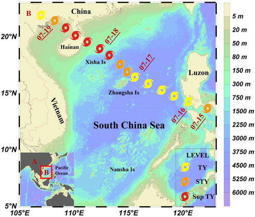
Figure 1 shows the research area of the SCS (5°−23°N, 105°−123°E), and the asterisk represents the best track (http://tcdata.typhoon.org.cn/zjljsjj_zlhq.html) of typhoon Rammasun. According to the Saffir-Simpson scale, typhoon Rammasun, a Category 4 super typhoon, was formed on 12 July 2014, at about 210 km west of Guam, USA, with its central position located at 13.5°N, 144.6°E. Then, it moved northwestward during 13–14 July 2014 as a Category 1 typhoon. Rammasun landed in the Philippines and entered the SCS on 15 July 2014 as a Category 3 typhoon. It quickly gained strength and intensified to a Category 4 super typhoon at 00:00 UTC on 18 July 2014. It made landfall on Hainan Island, China, as a Category 4 super typhoon and then in Xuwen County, Guangdong Province, also as a Category 4 super typhoon. The national meteorological center of the China Meteorological Administration announced that typhoon Rammasun dissipated on 20 July 2014. It lingered in the SCS for 4 days with a maximum wind speed of 72 m s⁻¹ with about 18 h as a Category 4 super typhoon.

Fig. 1. The depth of the South China Sea and the best track of super typhoon Rammasun in 2014.

2.2. Data

Typhoon data were obtained from the China Typhoon website and best-track typhoon data were obtained from the Tropical Weather Cyclone Data Center of China Meteorological Administration (http://tcdata.typhoon.org.cn/zjljsjj_zlhq.html). These data included the maximum sustained surface wind speed and six-hourly latitude/longitude measurements of the position of the typhoon’s center.

The SSW and SST data were obtained from the European Centre for Medium-Range Weather Forecast(https://apps.ecmwf.int/datasets/data/interim-full-daily/levtype=sfc/), spatial resolution: 0.125^°×0.125^°, temporal resolution: 1 day. Daily SLA data with a one-third degree spatial resolution were obtained from archiving, the Mercator Ocean (http://marine.copernicus.eu/services-portfolio/access-to-products/). Precipitation data were retrieved from the Tropical Rainfall Measuring Mission (https://disc2.gesdisc.eosdis.nasa.gov/data/TRMM_L3/TRMM_3B42/), spatial resolution: 0.25^°×0.25^°, temporal resolution: 1 day. The MLD was downloaded from the Mercator Ocean (http://marine.copernicus.eu/services-portfolio/access-to-products/), spatial resolution: 0.25^°×0.25^°, temporal resolution: 1 day.

3. Results and discussion

3.1. Responses of SST, MLD, SLA, SSW and precipitation to Rammasun

Figure 2 shows the sea surface temperature anomaly (SSTA) from July 10 to 21, 2014, Figs. 3 and 4 present the mean fields for MLD, SLA, SSW and precipitation in July 2014.

Fig. 2. Values of SSTA (°C) before (10-a, 11-b, 12-c, 13-d, 14-e, 15-f day), during (16-g, 17-h, 18-i, 19-j day) and after (20-k, 21-n day) the typhoon from July 10 to 21, 2014.

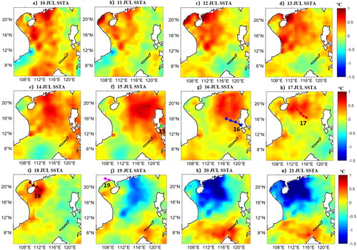
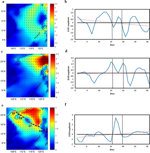
Fig. 3. The mean fields for sea surface MLD and SLA. (a) MLD (m), 1–15 July. (b) MLD (m), 16–31 July. (c) MLD (m), 20–23 July. (d) SLA (cm), 1–15 July. (e) SLA (cm), 16–31 July. (f) SLA (cm), 20–23 July. Contour intervals of the subfigures in the bottom row are 10 cm.

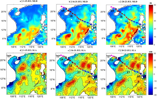
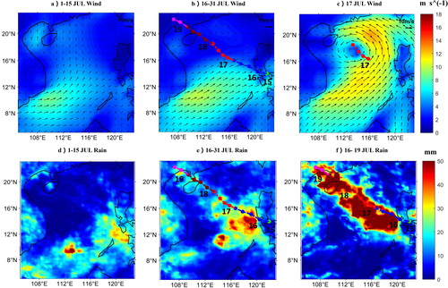
Fig. 4. The mean fields for SSW and precipitation. (a) SSW (m s^-1), 1–15 July. (b) SSW (m s^-1), 16–31 July. (c) SSW (m s^-1), 17 July. (d) Precipitation (mm), 1–15 July. (e) Precipitation (mm), 16–31 July. (f) Precipitation (mm), 16–19 July.

Figure 2 shows anomaly values of sea surface temperature (SSTA) before (Fig. 2a–f), during (Fig. 2g–j) and after (Fig. 2k, n) the typhoon from 10 to 21 July, 2014. From Fig. 2a–f, we can see that the SSTA in the NSCS was exceptionally high before the typhoon, providing a favorable underlying surface and energy source for typhoon strengthening in the NSCS. The shape of the SSTA distribution in southeast Vietnam (Fig. 2a and b) was called the ‘cold filament’ by Xie et al. (2003) and the ‘jet-shaped region’ by Zhao and Tang (2007). It is usually called a ‘cold spout’; this area of low SSTA is recognized to have upwellings and eddies (Fang et al., 2002; Zhao and Tang, 2007). Typhoon Rammasun entered the SCS on 16 July and progressed northwestward, causing a slight decrement of SST (Fig. 2g). The maximum cooling response of SST often poses a delayed time to the typhoon as many studies recognized (Bond et al., 2010; Tsai et al., 2012). The same results in our study were revealed in Fig. 2j, and a significant SST cooling occurred 3 days after typhoon’s landfall. Specifically, a remarkable cooling of the SST (like a cold pool) in the SCS had a clear ‘right-hand-side’ intensification for the typhoon track in the NSCS as shown in Fig. 2(j, k, n).

The MLD was deepened after the typhoon by comparing Fig. 3a and b. In line with the existing studies (Wu and Chen, 2012), there is a significant delay response of the upper ocean to the typhoon regarding MLD (Fig. 3c). The average MLD in the SCS increased to 21.80 m after the passage of the typhoon, compared with an average depth of 18.28 m before the typhoon, a rise of 19.3%. With 14°N as the dividing line, the average MLD in the NSCS increased from 13.66 m before the typhoon to 18.03 m after the passage of the typhoon, a rise of 32%, while the average MLD in the southern SCS (SSCS) increased from 22.78 m before the typhoon to 25.46 m after the passage of the typhoon, a change of 11.7%. Thus, the change in the MLD during the passage of the typhoon was much greater in the NSCS than in the SSCS. The change of MLD in the ocean has a great influence on the exchange of momentum, heat and mass between the atmosphere and the ocean (Clémen et al., 2004), and also plays major roles on nutrients and dissolved oxygen in biological and ecological research in the upper ocean (Morel and André, 1991; Longhurst, 1995; Polovina et al., 1995; Marty and Chiavérini, 2010; Auger et al., 2014).

Before the typhoon occurred, regions of negative SLA (cold eddies) existed mainly along with the western and northern parts of the SCS, especially in the Beibu Gulf and the Mekong estuary (Fig. 3d). There were three areas of positive SLA (warm eddies) in the SCS, located on the left and right side of Zhongsha Island east of Vietnam (Fig. 3d). An extremely important cold eddy was observed north of Zhongsha Island (Fig. 3d). These eddies are likely related to the SCS circulation and the Kuroshio, especially in the summer (Nan et al., 2011; Zheng et al., 2011). A ‘jet-shaped region’ of negative SLA was observed on the southeast coast of Vietnam. On the whole, compared with the SLA before and after the typhoon, the negative SLA areas were weakened, while the positive SLA areas were strengthened except for the warm eddy west of Zhongsha Island as shown in Fig. 3(d–f). The average SLA in the SCS increased from 3.51 cm before the typhoon to 3.71 cm after the typhoon.

Generally, the SCS is controlled by southwesterly winds in the summer. The winds were stronger in the south, weaker in the north and strongest off the coast of southeast Vietnam before the typhoon (Fig. 4a), resulting in a ‘jet-shaped region’ of SST and SLA with upwelling and eddies (Xie et al., 2003; Nan et al., 2011; Zheng et al., 2011). The typhoon enhanced this process (Fig. 4b), especially on 17 July 2014 (Fig. 4c), forming a cyclone wind field that was stronger to the right than to the left of the typhoon track. Unfortunately, ERA-Interim products did not acquire the actual wind speed during the typhoon period, but the actual maximal wind speed was 72 m s⁻¹. Before the typhoon, there was regional rainfall in the SSCS. After the typhoon, the rainfall mainly happened in the central and eastern of SCS near to the Philippines. But during the typhoon Rammasun, there was heavy rainfall along the track with strong left bias (Fig. 4d–f).

3.2. Spatiotemporal variations of SST, MLD, SLA, SSW and precipitation

Daily mean values of July in 15-year (2000–2014) datasets (SST, MLD, SLA, SSW and precipitation) were used as climatology data. The data used for the analysis below obtained by removing the climatology data and mean value from datasets of July in 2014. The EOFs of the dataset were calculated to reveal the daily variability of them over the SCS.

3.2.1. Spatial and temporal variability of SST

The contributions of the four leading modes of SST are shown in Table 1. Note that the first leading mode of SST accounted for 58.42% of the total variance. Below, we present our interpretation of the first leading mode. The spatial and temporal modes are shown in Fig. 5a and b, respectively. The first temporal mode of SST was dominated by the typhoon and reached peaks on 22 and 25 July. Before 18 July, the temporal mode was negative; however, the daily oscillation was reversed on 19 July. From 19 July, the daily oscillation was maintained positive, indicating a beginning of the continuing influence of the typhoon on the SST over the SCS and resulting in a three-day delay in the maximum cooling SST. In need of special is that another peak reached on 25 July could be the additional effect of the typhoon Matmo (2014). The spatial mode was characterized by the distribution of the SST cooling caused by the typhoon over the SCS. The spatial mode (Fig. 5a) was similar to that shown in Fig. 2 (j, k, n), with a clear ‘right-hand-side intensification’ of the SSTA relative to the typhoon track (Stramma et al., 1986; Sanford et al., 1987; Wada, 2005; D’Asaro et al., 2007), and there was an area of SSTA in eastern Vietnam. The spatial mode of EOF-1 indicated that when the temporal mode of EOF-1 became positive, the SSTA over the SCS displayed the temporal variability caused by Rammasun.

Fig. 5. The spatial mode (a) and temporal mode (b) of the first diurnal empirical orthogonal function of the sea surface temperature from 1–31 July 2014.

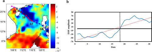
Table 1. Contributions (1–4) of diurnal empirical orthogonal function modes to SST, SLA, MLD, SSW and precipitation, the fifth column indicates the residual (Res) from the first four modes.

Mode	1	2	3	4	(Res)
(SST) Variance contribution (%)	58.42	15.94	7.7	Nan	17.94
(SLA) Variance contribution (%)	54.94	22.21	10.02	5.61	7.22
(MLD) Variance contribution (%)	28.19	18.42	12.92	9.57	30.90
(SSW) Variance contribution (%)	28.45	23.44	11.67	8.46	27.98
(Precipitation) Variance contribution (%)	13.68	10.31	8.90	7.28	59.83

Nan isn’t passing the 95% level of a significance test.

3.2.2. Spatial and temporal variability of SLA

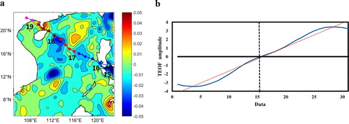
The contributions of the four leading modes of SLA are shown in Table 1. The first leading mode of SLA accounted for 54.94% of the total variance. The spatial and temporal modes are presented in Fig. 6a and b, respectively. The first temporal mode was dominated by the typhoon and reached a maximum on 28 July. The temporal mode was negative before the typhoon, but the diurnal oscillation reversed to be positive from 16 July on, indicating a continuing influence of the typhoon on the SLA over the SCS. A strong negative center in the southeast of Vietnam, two negative centers along the track of the typhoon and a positive center in the NSCS were observed. The spatial mode (Fig. 6a) was not similar to the pattern in Fig. 3d–f, indicating the movement of eddies over the SCS during the typhoon. The spatial mode of EOF-1 suggested that the SLA variation over the SCS caused by Rammasun when the temporal mode of EOF-1 changed from negative to positive (Fig. 6b).

Fig. 6. The spatial mode (a) and the temporal mode (b) of the first diurnal empirical orthogonal function of the surface level anomaly from 1–31 July 2014.

3.2.3. Spatial and temporal variability of MLD

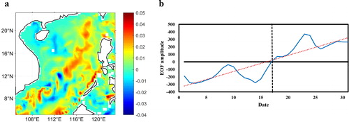
Table 1 shows the contributions of the four leading modes of MLD. The first leading mode of MLD accounted for 28.19% of the total variance. The spatial and temporal modes are shown in Fig. 7a and b, respectively. The first temporal mode was also dominated by the typhoon and reached peaks on 18 and 24 July. The temporal mode was negative before the typhoon but reversed on 17 July. The oscillation of MLD remained positive after 17 July, implying that the typhoon Rammasun deepened the MLD and thus introduced thermal energy into the upper layer, and another peak reached on 24 July could also be the additional effect of the typhoon Matmo (2014). The spatial mode (Fig. 7a) was similar in pattern to Fig. 3b, suggesting that vertical mixing of the upper ocean intensified over the SCS. The spatial mode of EOF-1 indicated that when the temporal mode of EOF-1 became positive, the MLD anomaly over the SCS displayed daily variability incurred by Rammasun.

Fig. 7. The spatial mode (a) and temporal mode (b) of the first diurnal empirical orthogonal function of the mixed layer depth from 1–31 July 2014.

3.2.4. Spatial and temporal variability of precipitation

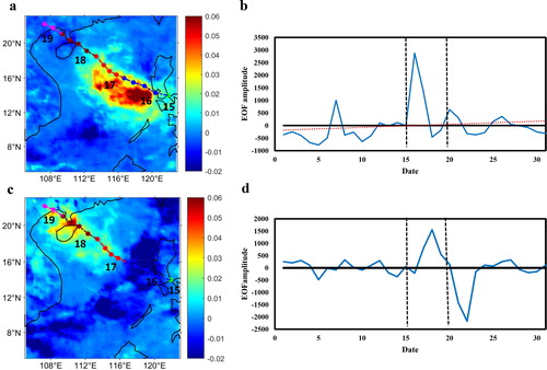
The contributions of the four leading modes of precipitation are listed in Table 1. The third and fourth leading modes of precipitation accounted for 8.90 and 7.28% of the total variance, respectively (i.e. less than 10%). Therefore, below we present our interpretation of the first and second leading modes. The first spatial and temporal modes are depicted in Fig. 8a and b, respectively. The first temporal mode was dominated by the typhoon and reached a maximum on 17 July. The temporal mode was maximally positive on 17 July and had only small amplitudes at other times. The spatial mode (Fig. 8a) was characterized by the distribution of the precipitation from 16–17 July, displaying a clear ‘left-hand-side intensification’ relative to the typhoon track (Lonfat et al., 2004; Chen et al., 2006). The second spatial and temporal modes are shown in Fig. 8c and d, respectively. The second temporal mode was also dominated by the typhoon and reached a maximum on 18 July. The temporal mode was maximally positive on 17 July. The spatial mode (Fig. 8c) was characterized by the distribution of the precipitation from July 17 to 18, having a clear ‘left-hand-side intensification’ relative to the typhoon track. Combining the first and second spatial modes reflected the distribution of the precipitation caused by the typhoon well, showing good consistency with the precipitation variability (Fig. 4f).

Fig. 8. The spatial modes (a and c) and temporal modes (b and d) of the first (a and b) and second (c and d) diurnal empirical orthogonal function of precipitation from 1–31 July 2014.

3.2.5. Spatial and temporal variability of SSW

Table 1 presents the contributions of the four leading modes of SSW. The fourth leading mode of SSW accounted for only 8.46% of the total variance (less than 10%), thus we interpreted the first three leading modes. The first and second temporal modes (Fig. 9b and d, respectively) were frequent diurnal fluctuations that did not highlight the effect of the typhoon. The first spatial mode contained a region with high wind anomalies in Taiwan Island. Similarly, the second spatial mode contained an area with high wind anomalies located in the eastern SCS. Although the first and second modes were not dominated by the typhoon, the third mode was characterized by the distribution of the SSW on 17 July (Figs. 4c and 9e–f) and had a clear ‘right-hand-side intensification’ concerning the typhoon track. The third temporal mode was dominated by the typhoon and reached a positive maximum on 17 July, showing only small amplitudes at other times.

Fig. 9. The spatial mode (a, c and e) and temporal mode (b, d and f) of the first (a and b), second (c and d) and third (e and f) diurnal empirical orthogonal function modes of sea surface wind from 1–31 July 2014.

3.3. Correlation analysis

The average variation of SST, MLD, SLA, SSW and precipitation with time is shown in Fig. 10. A normalization method was adopted to facilitate comparison. On the whole, the temporal variability of SST showed a significant negative correlation (−0.83) with MLD (Table 2). This means that a cooler SST was accompanied by a deeper MLD, and this was mainly attributed to the vertical mixing induced by the SSW. The temporal variability of MLD showed a significant positive correlation (0.74) with SSW (Table 2).

Fig. 10. Normalized average variation of SST, MLD, SLA, SSW and precipitation of the South China Sea (105°–123°E, 5°–23°N) in July 2014.

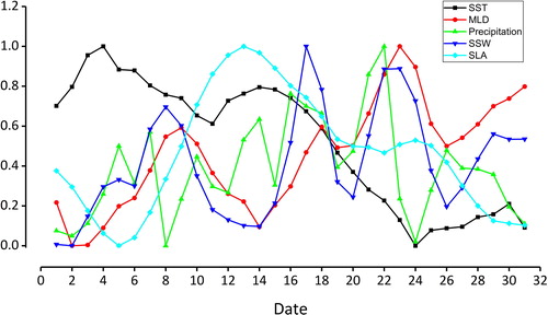
Table 2. Correlation analysis of the average variation of SST, MLD, SSW, SLA and precipitation of the South China Sea.

	SST	MLD	Precipitation	SSW	SLA
SST	1	−0.83	−0.02	−0.36	0.13
MLD		1	0.09	0.74	0.11
Precipitation			1	0.29	0.31
SSW				1	−0.10
SLA					1

The relationships between the time coefficient functions of the EOF modes of SST, MLD, SLA, SSW and precipitation for different numbers of lag days are shown in Fig. 11. The correlation coefficients between pairs of SST, MLD, SLA, SSW and precipitation are listed in Table 3. We selected the mean EOF-1 and EOF-2 modes of precipitation and the EOF-3 mode of SSW to reveal the effect of the typhoon. Overall, the time coefficient function of the EOF mode of SST lagged that of SSW by 3 days but remained in sync with that of MLD and SLA with SST. There was no notable correlation between the time coefficient function of the EOF mode of SST and that of precipitation (the highest correlation coefficient was 0.28 with a lag of 4 days). The time coefficient function of the EOF mode of SST showed a significant relationship with those of MLD and SLA, with correlation coefficients of 0.94 and 0.89, respectively. The time coefficient function of the EOF mode of MLD also exhibited a relationship with those of SLA (a correlation coefficient of 0.89) and precipitation (a correlation coefficient of 0.37). The time coefficient function of the EOF mode of precipitation also showed a correlation with that of SSW (a correlation coefficient of 0.55). Overall, the correlation between SST and MLD was good, while the correlations between the other physical quantities were much weaker, indicating that strong mixing during the typhoon may be an important reason for the continuous decline of SST.

Fig. 11. The correlations of the time coefficient functions for different lag days. (a) Time coefficient functions of the EOF-1 modes of SST and MLD. (b) Time coefficient functions of the EOF-1 modes of SST and surface level anomaly (SLA). (c) Time coefficient functions of the EOF-1 mode of SST and the mean of the EOF-1 and EOF-2 modes of precipitation. (d) Time coefficient functions of the EOF-1 mode of SST and the EOF-3 mode of SSW.

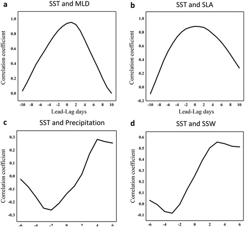
Table 3. Correlations of the time coefficient functions of the EOF modes of SST, MLD, SSW, SLA and precipitation.

Correlation	SST	MLD	Precipitation	SSW	SLA
SST	1	0.94	−0.14	0.25	0.89
MLD		1	−0.10	0.37	0.89
Precipitation			1	0.55	0.05
SSW				1	0.34
SLA					1

4. Discussion and conclusions

In this study, the anomalous oceanic conditions in the SCS during super typhoon Rammasun have been investigated using satellite observations or model data of SST, MLD, SLA, precipitation and a reanalysis of SSW. The EOF method was used to study the roles of variability in the SCS during July 2014. The major anomalous oceanic characteristic during super typhoon Rammasun was SST cooling after the typhoon’s passage. Assessments of the daily variabilities of SST, MLD, SLA, SSW and precipitation and the relationships between them during the period of the typhoon yielded the following results:

After typhoon Rammasun had passed through the SCS in July 2014, the maximal SST cooling exhibited a clear ‘right-hand-side intensification’ (Stramma et al., 1986; Wada, 2005; Wu et al., 2019) while heavy precipitation showed an obvious ‘left-hand-side intensification’ (Chen et al., 2006; Zhang et al., 2019) with respect to the typhoon track. The SST response exhibited obvious rightward biases because of the rotation resonance of the wind vector with wind-driven inertial currents (Yue et al., 2018), and precipitation response showed significant leftward biases due to vertical wind shear (Chen et al., 2006; Lin and Oey, 2016).

1. After the typhoon, the average MLD showed a notable positive relationship with SSW (0.74), while the inverse relationship with SST (−0.83), which increased more significantly in the NSCS (by 32%) than in the SSCS (by 11.7%). MLD has a good correlation with SSW and SST, respectively. Therefore, the strong wind caused by the typhoon can make deepen the MLD (Wu and Chen, 2012; Pan and Sun, 2013), and strong mixing was an important reason for the continuous decline of SST in this incident (Zhang et al., 2016; Yue et al., 2018).

2. The changes of SST between MLD and SLA were almost synchronous, while SST lagged that of SSW by 3 days based on the time coefficient functions of the EOF modes of SST, MLD, SLA, SSW. And the time coefficient function of the EOF mode of SST showed a significant relationship with those of MLD and SLA, with correlation coefficients of 0.94 and 0.89, respectively.

It should be aware that there are some limitations to our study. First, this is only a typhoon case study. To generalize the findings presented above, a large sample of the typhoon (and extratropical storms) should be collected and analyzed. This is true and necessary for analyzing of the typhoon. Second, the EOF result is sensitive. When analyzing a typhoon case, it may be affected by nearby typhoons. Therefore, the choice of typhoon cases has certain limitations. Also, choosing typhoons in different areas (except SCS) whether may produce different results. In response to the above issues, there are more cases that we need to be verified in the future.

Nonetheless, having stated the findings and limitations of the present study, we think it might be useful to analyze typhoons by using the EOF method for future research. Generally speaking, it is used to reduce any complicated data set into a finite and small number of new variables (Aliyu et al., 2019), meanwhile, it can be used to identify and separate the dominant and the underlying processes and essential parameters (Yosef et al., 2017). The spatial EOFs depict locations contributing most strongly to the respective principal components (Singarayer and Bamber, 2003), the time EOFs can see the long-term response of marine environmental parameters to typhoons (Figs. 5–7). And the use of EOF analysis can reveal the main impact of the typhoon as much as possible, as long as the contribution rate of the main mode is greater, the more the typhoon may affect this variable. Furthermore, EOF analysis can capture the most critical factors affecting changes caused by typhoons.

Acknowledgments

We thank two anonymous reviewers whose valuable comments and suggestions have helped to improve the manuscript. The SSW and SST data were kindly provided by ECMWF. Daily SLA and MLD data were obtained from the Mercator Ocean. Precipitation data were retrieved from the Tropical Rainfall Measuring Mission.

Disclosure statement

The authors declare that they have no conflict of interest.

Correction Statement

This article has been republished with minor changes. These changes do not impact the academic content of the article.

Additional information

Funding

This work was partially supported by the National Marine Important Charity Special Foundation of China no. 201305019; Error! Hyperlink reference not valid. no. 2014A030313603; Science and Technology Planning Project of Guangdong Province no. 2013B030200002; Innovation and Strong School Project of GDOU no. GDOU2014050226 and 20160222; Climbing Project of Guangdong Province no. pdjh2015b0249; and Humanity and Social Science Youth Foundation of the Ministry of Education of China no. 17YJCZH168.

References

- Aliyu, R., Tijjani, B. I. and Sharafa, S. B. 2019. Assessment and comparison of MODIS AOD and AE product over Ilorin Aeronet station using the statistical analysis of empirical orthogonal function (EOF). Bayero J. Pure App. Sci. 11, 223–229. doi:10.4314/bajopas.v11i1.37S
- Auger, P. A., Ulses, C., Estournel, C., Stemmann, L., Somot, S. and co-authors. 2014. Interannual control of plankton communities by deep winter mixing and prey/predator interactions in the New Mediterranean: Results from a 30-year 3d modeling study. Prog. Oceanogr. 124, 12–27. doi:10.1016/j.pocean.2014.04.004
- Bond, N. A., Cronin, M. F. and Garvert, M. 2010. Atmospheric sensitivity to SST near the Kuroshio extension during the extratropical transition of typhoon Tokage. Mon. Wea. Rev. 138, 2644–2663. doi:10.1175/2010MWR3198.1
- Chen, S. S., Knaff, J. A. Jr, and Marks, F. D. 2006. Effects of vertical wind shear and storm motion on tropical cyclone rainfall asymmetries deduced from TRMM. Mon. Wea. Rev. 134, 3190–3208. doi:10.1175/MWR3245.1
- Chen, X., Pan, D., He, X., Bai, Y. and Wang, D. 2011. Phytoplankton bloom and sea surface cooling induced by Category 5Typhoon Megi in the South China Sea: direct multi-satellite observation. In Remote Sensing of the Ocean, Sea Ice, Coastal Waters, and Large Water Regions (Vol. 8175). International Society for Optics and Photonics. p. 817519. doi:10.1117/12.897853
- Chu, C. 1979. Physical Geography of China-Ocean Geography. Science Press, Beijing (in Chinese).
- Chu, P., Edmons, N. and Fan, C. 1999. Dynamical mechanisms for the South China Sea seasonal circulation and thermohaline variabilities. J. Phys. Oceanogr. 29, 2971–2989. doi:10.1175/1520-0485(1999)029<2971:DMFTSC>2.0.CO;2
- Chu, P. C., Veneziano, J. M., Fan, C., Carron, M. J. and Liu, W. T. 2000. Response of the South China Sea to tropical cyclone Ernie 1996. J. Geophys. Res. 105, 13991–14009. doi:10.1029/2000JC900035
- Clément, D. B. M., Madec, G., Fischer, A. S., Lazar, A. and Iudicone, D. 2004. Mixed layer depth over the global ocean: an examination of profile data and a profile‐based climatology. J. Geophys. Res. Oceans 109, C12003. doi:10.1029/2004JC002378
- D’Asaro, E. A., Sanford, T. B., Niiler, P. P. and Terrill, E. J. 2007. Cold wake of hurricane frances. Geophys. Res. Lett. 34, 15609. doi:10.1029/2007GL030160
- Emanuel, K. A. 1986. An air-sea interaction theory for tropical cyclones. Part I: Steady-state maintenance. J. Atmos. Sci. 43, 585–605. doi:10.1175/1520-0469(1986)043<0585:AASITF>2.0.CO;2
- Emanuel, K. A. 1988. The maximum intensity of hurricanes. J. Atmos. Sci. 45, 1143–1155. doi:10.1175/1520-0469(1988)045<1143:TMIOH>2.0.CO;2
- Fang, W., Fang, G., Shi, P., Huang, Q. and Xie, Q. 2002. Seasonal structures of upper layer circulation in the southern South China Sea from in situ observations. J. Geophys. Res. 107, 23–1–23-12. doi:10.1029/2002JC001343
- Fu, D. Y., Luan, H., Pan, D. L., Zhang, Y., Wang, L. A. and co-authors. 2016. Impact of two typhoons on the marine environment in the Yellow Sea and East China Sea. Chin. J. Ocean. Limnol. 34, 871–884. doi:10.1007/s00343-016-5049-6
- He, J., Guan, Z. and Nong, M. 2008. Primary study on structure of wintertime typhoon Nanmadol in 2004. J. Trop. Meteorol. 24, 51–58. (in Chinese).
- Hu, J. Y. and Kawamura, H. 2004. Detection of cyclonic eddy generated by looping tropical cyclone in the northern South China Sea: a case study. Acta Oceanolog. Sin. 2, 002.
- Ko, D. S., Chao, S. Y., Wu, C. C. and Lin, I. I. 2014. Impacts of typhoon Megi (2010) on the South China Sea. J. Geophys. Res. Oceans 119, 4474–4489. doi:10.1002/2013JC009785
- Lau, K. M., Ding, Y., Wang, J. T., Johnson, R., Keenan, T. and co-authors. 2000. A Report of the field operations and early results of the South China Sea Monsoon experiment (SCSMEX). Bull. Amer. Meteor. Soc. 81, 1261–1270. doi:10.1175/1520-0477(2000)081<1261:AROTFO>2.3.CO;2
- Lin, I. I., Liu, W. T., Wu, C. C., Chiang, J. C. H. and Sui, C. H. 2003. Satellite observations of modulation of surface winds by typhoon-induced upper ocean cooling. Geophys. Res. Lett. 30, 31–31. doi:10.1029/2002GL015674
- Lin, Y. C. and Oey, L. Y. 2016. Rainfall-enhanced blooming in typhoon wakes. Sci. Rep. 6, 31310. doi:10.1038/srep31310
- Liu, Q., Jiang, X., Xie, S. P. and Liu, W. T. 2004. A gap in the Indo-Pacific warm pool over the South China Sea in boreal winter: Seasonal development and interannual variability. J. Geophys. Res. 109, C07012. doi:10.1029/2003JC002179
- Li, X., Fu, D. Y. and Zhang, Y. 2016. The impacts of super typhoon Rammasun on the environment of the northwestern South China Sea. J. Trop. Oceanog. 35, 19–28. (in Chinese).
- Li, Y. X., Yang, Y. J., Sun, L. and Fu, Y. F. 2014. The upper ocean environment responses to typhoon Prapiroon (2012). In Ocean Remote Sensing and Monitoring from Space (Vol. 9261). International Society for Optics and Photonics, p. 92610U. doi:10.1117/12.2069263
- Lonfat, M. J., Mark, F. D. and Chen, S. S. 2004. Precipitation distribution in tropical cyclones using the tropical rainfall measuring mission (TRMM) microwave imager: A global perspective. Mon. Wea. Rev.132, 1645–1660. doi:10.1175/1520-0493(2004)132<1645:PDITCU>2.0.CO;2
- Longhurst, A. 1995. Seasonal cycles of pelagic production and consumption. Prog. Oceanogr. 36, 77–167. doi:10.1016/0079-6611(95)00015-1
- Marra, J., Bidigare, R. R. and Dickey, T. D. 1990. Nutrients and mixing, chlorophyll and phytoplankton growth. Deep Sea Res. A 37, 127–143. doi:10.1016/0198-0149(90)90032-Q
- Marty, J. C. and Chiavérini, J. 2010. Hydrological changes in the Ligurian Sea (NW Mediterranean, DYFAMED site) during 1995–2007 and biogeochemical consequences. Biogeosciences 7, 2117–2128. doi:10.5194/bg-7-2117-2010
- Mei, W., Lien, C. C., Lin, I. I. and Xie, S. P. 2015. Tropical cyclone-induced ocean response: A comparative study of the South China Sea and tropical northwest pacific. J. Climate 28, 5952–5968. doi:10.1175/JCLI-D-14-00651.1
- Metzger, E. J. and Hurlburt, H. E. 2001. The Nondeterministic Nature of Kuroshio Penetration and Eddy Shedding in the South China Sea. J. Phys. Oceanogr. 31, 1712–1732. doi:10.1175/1520-0485(2001)031<1712:TNNOKP>2.0.CO;2
- Morel, A. and André, J. M. 1991. Pigment distribution and primary production in the western Mediterranean as derived and modeled from coastal zone color scanner observations. J. Geophys. Res. 96, 12685–12698. doi:10.1029/91JC00788
- Nan, F., He, Z., Zhou, H. and Wang, D. 2011. Three long‐lived anticyclonic eddies in the northern South China Sea. J. Geophys. Res. 116, 879–889. doi:10.1029/2010JC006790
- North, G. R., Bell, T. L., Cahalan, R. F. and Moeng, F. J. 1982. Sampling errors in the estimation of empirical orthogonal functions. Mon. Wea. Rev. 110, 699–706. doi:10.1175/1520-0493(1982)110<0699:SEITEO>2.0.CO;2
- Pan, J. and Sun, Y. 2013. Estimate of Ocean Mixed Layer Deepening after a Typhoon Passage over the South China Sea by Using Satellite Data. J. Phys. Oceanogr. 43, 498–506. doi:10.1175/JPO-D-12-01.1
- Polovina, J. J., Mitchum, G. T. and Evans, G. T. 1995. Decadal and basin-scale variation in mixed layer depth and the impact on biological production in the central and north pacific, 1960-88. Deep-Sea Research I 42, 0–1716.
- Price, J. F. 1981. Upper ocean response to a hurricane. J. Phys. Oceanogr. 11, 153–175. doi:10.1175/1520-0485(1981)011<0153:UORTAH>2.0.CO;2
- Ren, F., Gleason, B. and Easterling, D. 2002. Typhoon impacts on china’s precipitation during 1957-1996. Adv. Atmos. Sci. 19, 943–952.
- Sanford, T. B., Black, P. G., Haustein, J. R., Feeney, J. W., Forristall, G. Z. and co-authors. 1987. Ocean response to a hurricane: I. Observations. J. Phys. Oceanogr. 17, 2065–2083. doi:10.1175/1520-0485(1987)017<2065:ORTAHP>2.0.CO;2
- Sanford, T. B., Price, J. F. and Girton, J. B. 2011. Upper-ocean response to hurricane Frances (2004) observed by profiling em-apex floats. J. Phys. Oceanogr. 41, 1041–1056. doi:10.1175/2010JPO4313.1
- Shang, S., Li, L., Sun, F., Wu, J., Hu, C. and co-authors. 2008. Changes of temperature and bio-optical properties in the South China Sea in response to Typhoon Lingling, 2001. Geophys. Res. Lett. 35, L10602.
- Singarayer, J. S. and Bamber, J. L. 2003. EOF analysis of three records of sea‐ice concentration spanning the last 30 years. Geophys. Res. Lett. 30, 1251. doi:10.1029/2002gl016640
- Stramma, L., Cornillon, P. and Price, J. F. 1986. Satellite observations of sea surface cooling by hurricanes. J. Geophys. Res. 91, 5031–5035. doi:10.1029/JC091iC04p05031
- Sun, L., Yang, Y. J. and Fu, Y. F. 2009. Impacts of typhoons on the Kuroshio large meander: Observation evidences. Atmos. Oceanic Sci. Lett. 2, 45–50. doi:10.1080/16742834.2009.11446772
- Tsai, Y., Chern, C. S. and Wang, J. 2012. Numerical study of typhoon-induced ocean thermal content variations on the northern shelf of the South China Sea. Cont. Shelf Res. 42, 64–77. doi:10.1016/j.csr.2012.05.004
- Wada, A. 2005. Numerical simulations of sea surface cooling by a mixed layer model during the passage of typhoon rex. J. Oceanogr. 61, 41–57. doi:10.1007/s10872-005-0018-2
- Walker, N., Leben, R. and Balasubramanian, S. 2005. Hurricane‐forced upwelling and chlorophyll A enhancement within cold‐core cyclones in the Gulf of Mexico. Geophys. Res. Lett. 32, L18610. doi:10.1029/2005GL023716
- Wang, G., Su, J., Ding, Y. and Chen, D. 2007. Tropical cyclone genesis over the South China Sea. J. Mar. Syst. 68, 318–326. doi:10.1016/j.jmarsys.2006.12.002
- Wu, Q. and Chen, D. 2012. Typhoon-induced variability of the oceanic surface mixed layer observed by argo floats in the Western North Pacific Ocean. Atmos. Ocean 50, 4–14. doi:10.1080/07055900.2012.712913
- Wu, Z., Jiang, C., Chen, J., Long, Y., Deng, B. and co-authors. 2019. Three-dimensional temperature field change in the South China Sea during typhoon Kai-tak (1213) based on a fully coupled atmosphere-wave-ocean model. Water 11, 140. doi:10.3390/w11010140
- Wyrtki, K. 1961. Physical Oceanography of Southeast Asian Waters. Scripps Institution of Oceanography. Naga Report 2, pp.195
- Xie, S. P., Xie, Q., Wang, D. and Liu, W. T. 2003. Summer upwelling in the south china sea and its role in regional climate variations. J. Geophys. Res. 108, 3261. doi:10.1029/2003JC001867
- Yang, Y. J., Sun, L., Liu, Q., Xian, T. and Fu, Y. F. 2010. The biophysical responses of the upper ocean to the typhoons Namtheun and Malou in 2004. Int. J. Remote Sens. 31, 4559–4568. doi:10.1080/01431161.2010.485140
- Yeh, T. C. 2002. Typhoon rainfall over Taiwan area: The empirical orthogonal function modes and their applications on the rainfall forecasting. Terr. Atmos. Ocean. Sci. 13, 449–468. doi:10.3319/TAO.2002.13.4.449(A)
- Yosef, G., Alpert, P., Price, C., Rotenberg, E. and Yakir, D. 2017. Using EOF analysis over a large area for assessing the climate impact of small-scale afforestation in a semiarid region. J. Appl. Meteor. Climatol. 56, 2545–2559. doi:10.1175/JAMC-D-16-0253.1
- Yue, X., Zhang, B., Liu, G., Li, X., Zhang, H. and co-authors. 2018. Upper ocean response to typhoon Kalmaegi and Sarika in the South China Sea from multiple-satellite observations and numerical simulations. Remote Sensing 10, 348. doi:10.3390/rs10020348
- Zhang, H., Chen, D., Zhou, L., Liu, X., Ding, T. and co-authors. 2016. Upper ocean response to typhoon kalmaegi (2014). J. Geophys. Res. Oceans 121, 6520–6535. doi:10.1002/2016JC012064
- Zhang, H., Liu, X., Wu, R., Liu, F., Yu, L. and co-authors. 2019. Ocean response to successive typhoons Sarika and Haima (2016) based on data acquired via multiple satellites and moored array. Remote Sens. 11, 2360. doi:10.3390/rs11202360
- Zhang, M. and Jie, A. N. 2007. EOF expansion in one rainstorm. Chin. J. Atmos. Sci. 31, 321.
- Zhao, H. and Tang, D. L. 2007. Effect of 1998 El Niño on the distribution of phytoplankton in the South China Sea. J. Geophys. Res. 112, C02017. doi:10.1029/2006JC003536
- Zhao, H., Tang, D. L. and Wang, Y. 2008. Comparison of phytoplankton blooms triggered by two typhoons with different intensities and translation speeds in the South China Sea. Mar. Ecol. Prog. Ser. 365, 57–65. doi:10.3354/meps07488
- Zheng, Q., Tai, C. K., Hu, J., Lin, H., Zhang, R. H. and co-authors. 2011. Satellite altimeter observations of nonlinear Rossby eddy–Kuroshio interaction at the Luzon Strait. J. Oceanogr. 67, 365–376. doi:10.1007/s10872-011-0035-2
- Zheng, Z. W., Ho, C. R. and Kuo, N. J. 2008. Importance of pre-existing oceanic conditions to upper ocean response induced by Super Typhoon Hai-Tang. Geophys. Res. Lett. 35, L20603. doi:10.1029/2008GL035524