Multi-nested WRF simulations for studying planetary boundary layer processes on the turbulence-permitting scale in a realistic mesoscale environment

Abstract

The Weather Research and Forecasting (WRF) model was applied in a nested configuration from a 2.7 km convection-permitting domain via grey-zone resolutions of 900 m and 300 m down to the 100 m turbulence-permitting scale. Based on sensitivity studies, this approach was optimized to investigate the evolution of small-scale processes in the PBL for a clear sky case during the HOPE experiment in western Germany on 24 April 2013. The results were compared with theoretical and experimental findings from literature and high-resolution lidar observations collected during the campaign. Simulations with parameterized turbulence were able to capture the temporal evolution of the PBL height, but almost no internal structure was simulated in the boundary layer. Only the turbulence-permitting simulations were capable of reproducing the morning transition from the stable nighttime to the daytime convective boundary layer and the following break-up into turbulent eddies. Comparisons with lidar data showed that the turbulence-permitting simulations reproduced the observed turbulence statistics. Nevertheless, the potential temperature in the boundary layer was 1 K cooler than observed, caused by a lower surface temperature mixed upward by the turbulent eddies. The simulated PBL height was underestimated by 200 m, reflected in a well-captured profile of specific humidity up to a height of 900 m and an overly strong decrease of moisture above. The general shape of the variance profiles of potential temperature and specific humidity were captured by the model. However, the simulated variability throughout the boundary layer was lower and the different heights of the variance peaks indicated that the model may not fully capture the turbulent processes at the top of the boundary layer. Identifying those systematic differences between nested simulations and observations demonstrated the value of this model approach for process studies and parameterization tests.

Keywords:

• boundary layer
• turbulence
• WRF
• large-eddy simulation
• lidar

1. Introduction

To investigate atmospheric processes in the planetary boundary layer (PBL) and its interaction with the free troposphere above, meteorologists have focused on either observations or simulations of the atmosphere for many years. However, PBL processes strongly depend on the characteristics of the underlying surface. Details of the influence of vegetation and soil characteristics on the atmospheric surface layer and the PBL were only treated in a simplified way within models. In recent years, the importance of the land surface for a realistic representation of processes in the PBL and its correct diurnal cycle is of increasing interest in science (e.g. Song and Wang, 2015; Williams and Torn, 2015; Lin and Cheng, 2016; Abdolghafoorian et al., 2017; De Kauwe et al., 2017; Green et al., 2017; Santanello et al., 2018).

Several measurement campaigns were launched to collect three-dimensional observations of humidity, temperature and wind to improve the understanding of the boundary layer processes and to evaluate the model results. These include the IHOP_2002¹ campaign (Weckwerth et al., 2004) along the central U.S. dryline, the LITFASS² experiment (Beyrich et al., 2006) around the observatory of the German Weather Service in Lindenberg southeast of Berlin, the COPS³ campaign over the low mountain regions of south-western Germany (Wulfmeyer et al., 2011), HOPE⁴ in spring 2013 (Macke et al., 2017) in western Germany, the SABLE⁵ campaign in summer 2014 north of the Black Forest in Germany (e.g. Behrendt et al., 2015; Hammann et al., 2015; Muppa et al., 2016; Späth et al., 2016; Di Girolamo et al., 2017), the ScaleX campaign on scale-crossing land surface and boundary layer processes in a pre-Alpine observatory 2015 and 2016 (Wolf et al., 2017) and LAFE⁶ in August 2017 in Oklahoma (USA) (Wulfmeyer et al., 2018).

Simultaneously, increasing computer performance allows for applying numerical models to improve the understanding of land surface - atmosphere (LA) interaction. Due to increased mesoscale model resolution, the explicit description of small-scale atmospheric processes and a more accurate description of the lower boundary in the simulations became possible. Currently, mesoscale models, applied for scientific as well as operational applications use horizontal resolutions of a few km. The increased horizontal resolution allows the explicit simulation of deep convection, leading to a more realistic representation of the temporal and spatial distribution of precipitation (e.g. Bauer et al., 2011; Schwitalla et al., 2011; Zittis et al., 2017; Feng et al., 2018; Martínez and Chaboureau, 2018; Woodhams et al., 2018). The more realistic representation of the land surface and the application of urban canopy models, in addition, allow the detailed investigation of the urban boundary layer, important in view of the growing number of city residents and the changing future climate (e.g. Song et al., 2018; Huang et al., 2019 or Teixeira et al., 2019).

A disadvantage of mesoscale models is their requirement for a turbulence parameterization even at the km scale. The most common approaches applied are local and non-local schemes that differ in the depth over which the turbulent fluxes affect the variables at a specific height within the PBL. Whereas the local approach only accounts for the impact of adjacent levels, the non-local approach also includes the mixing of the largest eddies in the PBL. In cases where the characteristics of turbulence including the LA interactions are investigated, grid sizes well below 1 km are required to explicitly resolve smaller processes.

In the resolution range between approximately 1.5 km and 200 m, the so-called ‘grey zone’ or ‘terra incognita’ (e.g. Wyngaard, 2004; Honnert et al., 2011), models start to resolve the larger turbulent eddies explicitly. The application of a turbulence scheme may therefore worsen the representation of the larger eddies, whilst remaining necessary to parameterize the smaller parts of the turbulent spectrum (Wyngaard, 2004; Honnert and Masson, 2014; Zhou et al., 2014; Efstathiou et al., 2016; Zhou et al., 2017).

Large eddy simulation (LES) models were developed and continuously improved during recent decades (e.g. Deardorff, 1974; Moeng, 1984; Chlond and Wolkau, 2000; Raasch and Schröter, 2001) to enable the implicit simulation of turbulence in the atmospheric boundary layer including the interaction with the land surface and the development of clouds and precipitation (e.g. Heinze et al., 2017). They are operated at resolutions down to meters and use a low-pass filter to split the energy cascade into resolved and non-resolved components. The former contains most of the energy carrying eddies, whereas the parameterized non-resolved part consists only of the small eddies, which are less important for energy transport in the boundary layer.

Traditionally, LES models were applied with periodic lateral boundary conditions and a homogenous lower boundary to investigate characteristics of turbulence in the PBL (e.g. Moeng, 1984; Chlond et al., 2004; Mirocha et al., 2010; Raasch and Franke, 2011). ‘Homogenous’ means that no orography or realistic descriptions of land cover and soil characteristics are applied. For example, the Dutch Atmospheric Large-Eddy Simulation model (DALES, Heus et al., 2010) and the Parallelized Large-Eddy Simulation model (PALM, https://palm.muk.uni-hannover.de), developed at the institute of Meteorology and Climatology of the University of Hannover (Maronga et al., 2015) are state-of-the-art models applied for idealized purposes. This approach helped to reveal important information about the temporal and spatial evolution of turbulence and its characteristics. However, interactions between a realistic land surface and the PBL cannot be investigated due to the homogenous lower boundary. This is possible when LES models are applied for real cases, namely for the investigation of turbulence above real orography and land cover conditions, driven by real meteorological forcing. Under these conditions, results can be studied in combination with observational data. For this purpose, tools such as the LES-cores of the Icosahedral Nonhydrostatic (ICON) model of the German Weather Service (Dipankar et al., 2015) and the LES mode in the Weather Research and Forecasting (WRF) model (Skamarock et al., 2008), applied in this study, were developed. The seamless nesting into mesoscale WRF using a self-contained and consistent set of physical parameterizations strongly reduces the inclusion of physical imbalances from the mesoscale to the LES simulation (e.g. Zhu, 2008a, 2008b; Zhu et al., 2010; Mazzaro et al., 2017; Muñoz-Esparza et al., 2017). Furthermore, the system can be applied for real cases when the mesoscale outer domain is driven by meteorological analyses or, even more realistically, when the initialization of the outer domain is further improved with data assimilation.

In this study, we apply a multi-nested WRF configuration to investigate the evolution of the atmospheric boundary layer at different horizontal resolutions. Our target grid spacing for the inner domain was 100 m. Since this is coarser than the typical resolutions applied for LES, we denote our simulations as turbulence-permitting (TP). With sensitivity studies of different model configurations, we optimize the model setup. To gain insight into the influence of LA feedback, the boundary layer evolution over different land use types is also investigated. Finally, the simulated evolution of turbulence is verified with high-resolution Raman and differential absorption lidar data.

The following scientific questions will be addressed:

• What is the optimal configuration of the multi-domain simulations for the application in the daytime convective boundary layer?

• What are the general advantages of this multi-nested approach compared to high-resolution mesoscale and/or idealized LES simulations? Is the grey zone more realistically represented using this approach?

• How is the temporal and spatial evolution of the boundary layer represented by the different resolutions in the applied multi-scale approach?

• Is the statistical evolution of turbulence realistically represented by the model? What is the benefit of an increase in resolution for the representation of turbulence statistics?

The manuscript is structured as follows. Section 2 introduces the selected case study, describes the model configuration and optimization, and explains the methodology to validate the model performance. Section 3 presents the results analyzing the spatial and temporal evolution of the boundary layer in the different domains of the multi-nested configuration. For this purpose, the horizontal evolution at different times, the temporal evolution at a lidar site and the comparison of turbulence statistics are applied. Section 4 discusses the results and relates them to findings of other studies. Section 5 summarizes the major results. This is done by answering the scientific questions posed at the end of the introduction. Finally, an outlook to possible future applications of the multi-nested configuration is given.

2. Case study and methodology

2.1. Case study

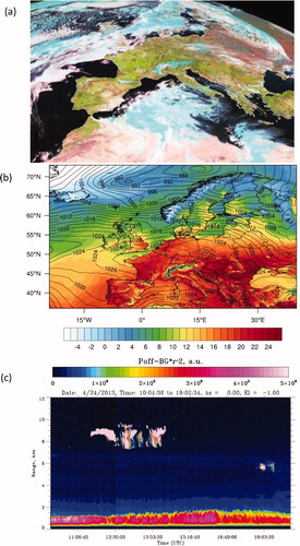
As a case study, the evolution of the convective boundary layer on April 24, 2013 was selected. It was a clear-sky day, allowing us to investigate the evolution of the convective boundary layer, undisturbed by clouds. The numerical simulation of clouds is a well-known challenge and complicates any comparison with observations. Figure 1 presents observations and ECMWF analysis data to summarize the synoptic situation. The synoptic situation was dominated by a high pressure system centered over southern Germany with almost no pressure gradients in large parts of central Europe. Low pressure systems travelled around the system over Scandinavia or the Mediterranean Sea, not influencing the region of interest in Western Germany. Wide-spread subsidence in the high pressure system resulted in almost no clouds formed in the region, as shown by the satellite image (Fig. 1a) and the time-height cross section of the lidar (Fig. 1c). Due to the clear and undisturbed conditions, this was a useful day to study the evolution of the boundary layer with only weak large-scale forcing.

Fig. 1. (a): ‘Natural color’ composite image of the Meteosat satellite (Source: NERC satellite receiving station, Dundee University) for 12 UTC, 24 April 2013. Clouds containing ice particles are colored in cyan. (b): Mean sea level pressure (contour) and near surface temperature from the ECMWF operational analysis with approximately 15 km horizontal resolution, providing the external forcing for the applied model chain. (c): Vertically-pointing range corrected backscatter signal at 820 nm wave length of the Hohenheim WVDIAL system.

2.2. Model configuration and initialization

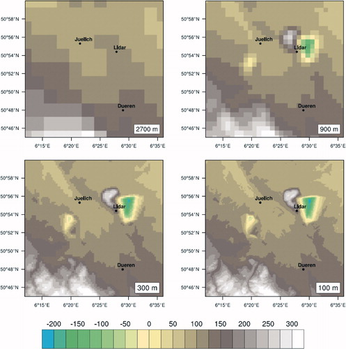
For the investigation, the WRF model in version 3.7.1 was applied. The domain configuration is shown in Fig. 2 – selected via a series of sensitivity tests, briefly described below. The outer domain (D01) with a horizontal resolution of 2700 m consists of 300 × 300 grid elements. Into this, three more nests with 900 m, 300 m and 100 m horizontal resolution were implemented to ensure a gradual downscaling to the target resolution of 100 m. The 900 m domain consists of 301 × 301 grid points, whilst the two inner domains were extended to 502 × 502 grid cells to provide a sufficiently large area of analysis, well away from the boundaries. The influence of the change in resolution on the model representation of the topography is shown in Fig. 3. The depression becoming visible with increasing resolution is the brown coal open pit ‘Hambach’. In the inner two domains D03 and D04, with 300 m and 100 m resolution, the turbulence parameterization was switched-off and the model was operated in TP mode. The larger size of the inner two domains provides the needed time and room to spin-up the turbulence (e.g. Mazzaro et al., 2017).

Fig. 2. Domain configuration of the WRF model chain. (a): Outer three domains with 2700 m resolution (D01), 900 m resolution (D02) and 300 m resolution (D03). (b): Domain 03 (300 m) including the inner domain with 100 m resolution.

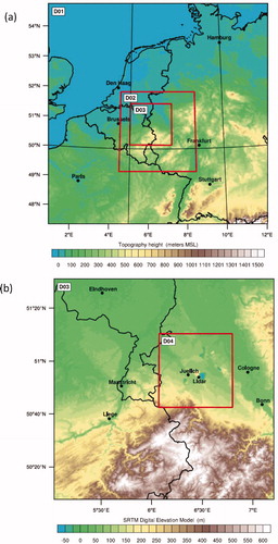
Fig. 3. Refinement of the representation of orography in the region of interest from 2700 m, 900 m, 300 m and 100 m. For the outer domain, the default data of the WRF pre-processing system (WPS) were used. The orography for the three inner domains were derived from the 90 m Shuttle Radar Topography Mission (SRTM) data set.

To adequately simulate the spatial and temporal evolution of the internal processes in the daytime boundary layer, high vertical resolution is needed. The vertical grid increment Δz needs to be the same or less than the horizontal grid increment Δx. Therefore, a stretched grid with 121 vertical levels up to a height of 50 hPa was applied for all four domains to ensure a well-represented troposphere. From the 121 levels, 30 to 35 are in the lowest 1500 m.

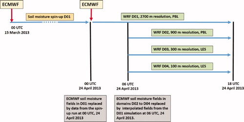
To overcome the well-known problem of soil equilibrium in cold start simulations (e.g. Cai et al., 2014), a spin-up simulation with the full WRF model was performed for the outer domain starting at 00 UTC March 15, 2013. The time line of the simulation set-up is shown in Fig. 4. The model chain was initialized at 00 UTC, 24 April 2013 with data from the operational analysis of the European Center for Medium-range Weather Forecasting (ECMWF). The analysis was created with the aid of a sophisticated global 4DVAR data assimilation system ensuring that the large-scale forcing of the simulation was as close as possible to the observation over the forecast range. The soil moisture and soil temperature fields were replaced by the values of the spin-up simulation. For the first 6 hours after initialization (until 06 UTC), only the outer 2.7 km domain was simulated. This ensures that the atmosphere is in balance with the new soil fields from the spin-up simulation, before providing the lateral boundary condition for the inner domains. In addition, the turbulence we aim to explore occurs later, meaning that the more computationally demanding inner domain simulations are not necessary for the first six hours. At 06 UTC, the initial conditions of soil moisture and soil temperature of the inner three domains were replaced by interpolated values from the outer domain. From 06 UTC to 18 UTC, all four domains were run simultaneously in a one-way nested configuration to allow a comparison of the evolution of the boundary layer in the different domains.

Fig. 4. Flow chart illustrating the setup of the model chain for the simulations.

The orography was initialized with data from the Shuttle Radar Topography Mission (SRTM, version 4) at a resolution of 3 arc seconds (approx. 90 m) (Farr et al., 2007; Reuter et al., 2007; Jarvis et al., 2008). The tiled data set was retrieved for central Europe from the webpage of the Center for Tropical Agriculture (CIAT, http://srtm.csi.cgiar.org). The geotiff files were merged with utilities of the Geospatial Data Abstraction Library (GDAL) and finally prepared for the WRF pre-processing system with the ‘convert_geotiff’ utility (available online at https://github.com/openwfm/convert_geotiff).

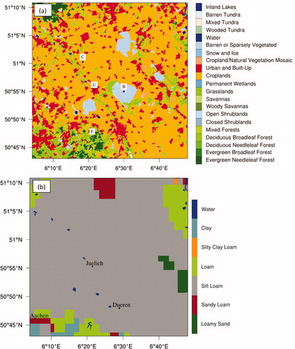
The CORINE land cover data set (Buettner, 1998; Buettner et al., 2002) with a resolution of 100 m was prepared for the use with the WRF pre-processing system (WPS). Since CORINE defines more land use classes than the MODIS data set available for the WRF pre-processing system, the preparation included a re-classification to the MODIS land cover categories to allow a straightforward implementation into the WRF pre-processing. This was done using a judicious merging of the appropriate categories within a Geographic Information System (GIS) software and the conversion to the WRF pre-processing system was again executed with the ‘convert_geotiff’ utility. Finally, the model was applied with the more sophisticated soil texture data set compiled by Milovac et al. (2014a, 2014b). It has a resolution of 1000 m and is based on a combination of the Harmonized World Soil Database (HWSD) and the German soil map in the scale 1:1000000 (Bodenübersichtskarte, BÜK1000). Figure 5 shows the applied land cover and soil maps for the innermost 100 m domain.

Fig. 5. Land use categories (100 m resolution) (a) and soil categories (1000 m resolution) (b) applied as lower boundary forcing for the WRF simulations.

We applied WRF with a previously tested set of physical schemes (e.g. Jankov et al., 2011; Balzarini et al., 2014; Schwitalla and Wulfmeyer, 2014; Cohen et al., 2015; Milovac et al., 2016). Cloud microphysics was parameterized with the Morrison 2-moment scheme (Morrison et al., 2009). Since we started our model chain with a horizontal resolution of 2700 m, deep convection was not parameterized. Shallow, non-precipitating convection was represented by a separate shallow convection scheme (GRIMS, Hong et al., 2013) in the outermost domain, to improve the vertical distribution of moisture from the convective boundary layer into the free troposphere. In the three inner domains, the scheme was switched-off. The RRTMG scheme (Iacono et al., 2008) was applied for shortwave and longwave radiation.

The land surface was simulated by the NOAHMP model (Niu et al., 2011) containing several options to describe land surface processes and the exchange with the boundary layer. A complete list of the NOAHMP namelist options, its meaning and the values selected for this study are presented in Table 1. For the surface layer, the revised MM5 Monin-Obukhov scheme (Jiménez et al., 2012) was applied. The planetary boundary layer (PBL) turbulence in the outer two domains with 2700 m and 900 m resolution was parameterized with the non-local YSU scheme (Hong et al., 2006). For the inner two domains with 300 m and 100 m resolution, the PBL scheme was switched-off and the model was operated in turbulence-permitting (TP) mode.

Table 1. Selected switches for the NOAHMP land surface model.

NOAHMP switch	Selected	Meaning
Dynamic Vegetation (dveg)	3	Dynamic vegetation model switched-off, leaf area index from table, vegetation fraction calculated
Canopy stomatal resistance (opt_crs)	1	Stomatal resistance with Ball-Berry scheme
Surface layer drag coefficient (opt_sfc)	1	Surface layer drag coefficient Monin-Obukhov
Soil moisture factor for stomatal resistance (opt_btr)	2	Soil moisture factor for stomatal resistance from the Common Land Model (CLM)
Runoff and ground water (opt_run)	3	Free drainage for runoff and subsurface runoff
Supercooled liquid water (opt_frz)	1	Supercooled liquid water (no iteration)
Frozen soil permeability (opt_inf)	2	Soil permeability (non-linear effects, less permeable)
Radiative transfer (opt_rad)	3	Radiative transfer (two-stream model applied to vegetated fraction)
Ground snow surface albedo (opt_alb)	1	Calculated with the BATS scheme
Participating precipitation rain/snow (opt_snf)	3	Snow for T < TFREEZE, rain elsewhere
Lower boundary soil temperature (opt_tbot)	2	Soil temperature lower boundary condition at 8 m from initial file
Snow/soil temperature time scheme (opt_stc)	1	Semi-implicit snow/soil temperature time scheme

The simulations were carried out on the high performance computing systems ForHLR 1 and bwUniCluster of the state of Baden-Wuerttemberg. With the Message Passing Interface, each simulation was distributed to 20 nodes containing 20 processing cores each, meaning a total of 400 compute cores were applied. An 18-hour simulation, starting at 00 UTC, 24 April 2013 took almost two days to complete (the outer domain only for the first 6 hours, followed by a 12-hour simulation of all four nests). The whole simulation output including hourly restart files for all four domains needed about two TB of disk space. For the sensitivity studies to find the optimal configuration, five more simulations and 10 to 15 TB of stored data were necessary. This demonstrates that such simulations are expensive, and require careful planning and effort even on high performance computing systems.

2.3. Turbulence-permitting simulations

The LES method applies a low pass filter to each of the flow field variables to separate the resolved and non-resolved parts of the turbulence spectrum. The effects of the non-resolved scales are contained in the subfilter-scale (SFS) stress. The SFS stresses and fluxes are usually parameterized using SFS models, providing temporally and spatially varying forcing for the explicitly resolved turbulent motion to accurately reproduce the drain in the energy cascade in a statistical sense. More details about the implementation of LES into WRF are, e.g., provided in Mirocha et al. (2010) and Kirkil et al. (2012). Many approaches of different complexity to describe the SFS stresses have been proposed in the past. The linear eddy-viscosity model (Smagorinsky, 1963) and a TKE-based approach (Deardorff, 1974) are well established in literature and widely used (e.g. Nakayama et al., 2008). These models, however, have been shown to be over-dissipative (e.g. Porté-Agel et al., 2000). We applied the 1.5 order TKE closure (Lilly, 1968) to represent the scalar fluxes and the nonlinear backscatter and anisotropy (NBA) model of Kosovic (1997) to represent the sub-grid scale momentum fluxes in the two inner model domains. Chen and Tong (2006) showed that the NBA model improves the representation of SFS stress as compared to the Smagorinsky model in simulations of the convective boundary layer since the important anisotropy of the shear stress is better resolved. Table 2 lists the namelist variables and their associated values illustrating the differences between the mesoscale and turbulence-permitting domains.

Table 2. Namelist configuration of the WRF-LES mode.

Namelist switch	D01 (2700 m )	D02 (900 m)	D03 (300 m)	D04 (100 m)
bl_pbl_physics	1	1	0	0
topo_wind	1	1	0	0
slope_rad	0	1	1	1
diff_opt	1	1	2	2
km_opt	4	4	2	2
mix_full_fields	.false.	.false.	.true.	.true.
sfs_opt	0	0	1	1

2.4. Optimization of the WRF-LES setup

During the preparation of the simulations, initial tests in the 100 m domain showed that the performance of WRF-LES strongly depends on the model set up. Therefore, sensitivity studies were performed and qualitatively assessed to determine the general setup of the model that lead to the most realistic development of turbulence in the innermost 100 m domain. Criteria were domain size, number of vertical levels, and the decision whether the WRF-LES mode or the usage of a PBL parameterization is better in the 300 m domain.

Figure 6 shows the representation of the vertical velocity approximately 1000 m above ground at the same time step for different model setups of the case selected in this study. The number of vertical levels used is 57 and 121, the domain size of the 100 m domain is 301 × 301 and 502 × 502 grid points and the 300 m domain was simulated with and without a PBL parameterization. The differences between the four setups are summarized in Table 3. This comparison shows that a large number of vertical levels (compare CTRL with EXP_A) and the use of the WRF-LES mode also in the 300 m domain (compare EXP_A with EXP_B) accelerates the initialization of turbulence in the innermost 100 m domain. A higher vertical resolution leads to a better representation of vertical transports and with a driving LES domain, resolved turbulence forces the inner domain. Mirocha et al. (2014) also found an improved setup of turbulence with a driving LES domain. A larger inner domain provides more space for the development of turbulence (compare CTRL, EXP_A and EXP_B with EXP_C). The transition regions along the inflow boundaries of the domain, in which the resolution adjustment from the outer to the inner domain takes place, appear narrower (lower right panel). This helps to ensure that the turbulence is fully developed in the region of interest in the 100 m domain. Based on the results and a series of further test runs (not shown), we decided to use 121 vertical levels in all four domains, we switched to LES mode also in the 300 m domain and we enlarged the inner two domains to 502 × 502 grid cells.

Fig. 6. Representation of vertical velocity 1000 m above sea level on April 24, 2013 at 13 UTC for four different model configurations. Shown is the innermost model domain with 100 m horizontal resolution. CTRL: 301 × 301 grid points with 57 vertical levels (15 in the boundary layer) and turbulence parameterization in the surrounding 300 m domain. EXP_A: As CTRL, but without turbulence parameterization in the 300 m domain. EXP_B: As EXP_A, but with 121 vertical levels (more than 30 in the boundary layer). EXP_C: As EXP_B, but with a larger domain size of 502 × 502 grid points. The green dot marks the location of the Hohenheim lidar systems.

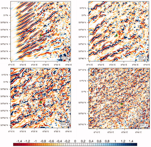
Table 3. Configuration of the different experiments to optimize the WRF-LES performance.

Experiment	No. of vertical levels (below 1500 m)	PBL scheme in D03	Dimension of D04 [Δx × Δy]	Domain size of D04 [km × km]
CTRL	57 (15)	yes	301 × 301	30.1 × 30.1
EXP_A	57 (15)	no	301 × 301	30.1 × 30.1
EXP_B	121 (>30)	no	301 × 301	30.1 × 30.1
EXP_C	121 (>30)	no	502 × 502	50.2 × 50.2

2.5. Measurement campaign and data for model verification

The purpose of HOPE was to collect high-resolution measurements focusing on the onset of clouds and precipitation in the convective boundary layer for both model verification and process studies (Macke et al., 2017).

The Institute of Physics and Meteorology (IPM) of the University of Hohenheim (UHOH) operated their water vapor differential absorption lidar (WVDIAL) (Muppa et al., 2016; Späth et al., 2016) and temperature rotational Raman lidar (TRRL) systems at a site close to the village of Hambach near the Research Center Juelich. An overview of these active remote sensing methodologies in comparison to other remote sensing techniques is presented in Wulfmeyer et al. (2015). Due to its high-power laser transmitter and a very efficient receiver, WVDIAL provides absolute humidity profiles with high temporal and spatial resolution of typically 1–10 s and 30–150 m, respectively. During HOPE, the WVDIAL was operated in vertical staring mode during clear sky conditions and in scanning mode during cloudy periods. In total, the instrument collected 180 hours of data during 18 days of intensive operations. A detailed description of the UHOH WVDIAL setup during HOPE and the derivation of the water vapor profiles is provided by Späth et al. (2016). High-resolution observations and their application for a better understanding of PBL turbulence statistics are presented in Muppa et al. (2016) and Wulfmeyer et al. (2016).

In recent years, the UHOH TRRL was upgraded to reach also turbulent resolution in the CBL. It was demonstrated that the TRRL measurements resolve not only the location and strength of the temperature inversion in the interfacial layer (Hammann et al., 2015) but also the measurements of profiles of the turbulent moments of temperature fluctuations up to the forth order (Behrendt et al., 2015; Wulfmeyer et al., 2016). During HOPE, daytime temperature profile measurements were provided by the system with high temporal and spatial resolution of typically 10 s and 105 m, respectively. Similar to WVDIAL, TRRL was operated in vertical staring mode during clear sky conditions and in scanning mode during cloudy periods and the amount of collected data is comparable to the WVDIAL. A detailed description of the UHOH TRRL setup during HOPE and the derivation of the water vapor mixing ratio and temperature profiles is provided by Hammann et al. (2015). High-resolution temperature observations and their application for a better understanding of PBL turbulence statistics are presented in Behrendt et al. (2015) and Muppa et al. (2016). In terms of spatial and temporal resolution and the way the different data sets are combined, the Hohenheim WVDIAL and the TRRL systems are worldwide unique instruments for turbulence studies and comparisons with LES (see Behrendt et al., 2015; Hammann et al., 2015; Wulfmeyer et al., 2015; Späth et al., 2016).

2.6. Methodology to compare with lidar data

The full model output for the domains was written every 5 minutes, which is by far not enough to resolve the temporal and spatial development of single turbulent eddies. For this, an output interval of the order of 10 s is necessary. This would require a huge increase in computational (I/O is expensive) and storage needs for the simulations. For instance, if a 1-hour simulation is restarted and the full model output is written every 10 s in the 100 m domain only, it takes 24 hours walltime to do the simulation and 3.5 TB of disk space are needed. This shows that careful planning and effort are necessary for such simulations even on high performance computing systems.

Despite these constraints, WRF allows the separate storage of time series of selected variables at selected grid cells at every model time step. Using this feature, time series of vertical profiles in the grid cell where the lidar systems, shown in Fig. 7, were located were stored (12 seconds, 4 seconds, 1.333 seconds and 0.44 seconds in the 2700 m, 900 m, 300 m and the innermost 100 m domain) in addition to the regular model output every five minutes. For comparisons of the different model resolutions, the time series data of the different domains were interpolated to 12 seconds, the time step of the coarsest domain. To compare the simulated and observed turbulence statistics, the mean and the variance were calculated for the time period 12 UTC to 14 UTC, 24 April 2013. The same time window was selected by Heinze et al. (2017) for intercomparisons of different instruments with the ICON-LES and COSMO model.

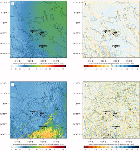
Fig. 7. Water vapor mixing ratio (g/kg) (panels a and c) and vertical velocity (m/s) (panels b and d) interpolated to 1000 m above sea level for 07 UTC (panels a and b) and 09 UTC (panels c and d), 24 April 2013.

The statistical moments were derived following the methodology of Lenschow et al. (2000) and Wulfmeyer et al. (2016). For each height level during the 2-hour window, the turbulent fluctuations are determined by subtracting a linear trend from the time series resulting in a fluctuating time series, e.g., water vapor mixing ratio q´(t). Subsequently, the higher-order moments such as the variance are calculated (Wulfmeyer et al. 2016).

3. Results

Firstly, we investigated the evolution of the convective boundary layer (CBL) in the 100 m domain with horizontal plots at four different times in Section 3.1 to assess the capability of the TP simulation to spin-up turbulence along the windward boundaries and represent the internal structure of the CBL in a realistic manner. Secondly, we focused on the temporal evolution of vertical profiles of moisture and the boundary layer structure, including the morning and early evening transitions in Section 3.2. Here, the performance of the different domains was compared with WVDIAL and TRRL observations (green dot in Fig. 6, ‘Lidar’ in Figs. 7 and 8). In addition, the influence of the underlying land surface was considered by investigating the evolution of the boundary layer over different land cover classes. Thirdly, in Section 3.3 it was investigated whether the statistics of turbulence are comparable to the lidar observations. To document the information gain of the increasing resolution, the coarser resolution simulations with 2700 m, 900 m and 300 m were included in the comparison.

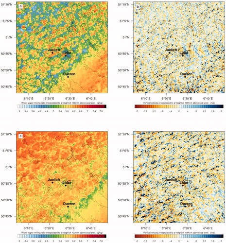
Fig. 8. Same as Figure 7, but for 12 UTC (panels a and b) and 15 UTC (panels c and d), 24 April 2013.

3.1. Horizontal evolution of the boundary layer

Figures 7 and 8 present the horizontal evolution of the boundary layer in the 100 m WRF-LES domain at four arbitrarily selected time steps during the diurnal development. For these time steps, we focused on the water vapor mixing ratio and the vertical wind velocity field to illustrate the horizontal evolution and mesoscale and turbulent transport processes.

Figure 7 shows the water vapor mixing ratio and the vertical velocity at 07 UTC (panels a and b) and 09 UTC (panels c and d) linearly interpolated to 1000 m above sea level (ASL). At 07 UTC, approximately one hour after sunrise and before the onset of turbulence, the boundary layer was still stably stratified, so that vertical velocities were small. Some orographically induced wave structures were simulated over the low mountain region in the southern part of the domain. Elsewhere, roll-like structures with alternating upward and downward motion directed perpendicular to the horizontal wind velocity (westerly) developed. In the water vapor mixing ratio, a west-to-east increase was visible related to a west-to-east decrease of the temperature (not shown), but no strong vertical transport of water vapor was present. The largest amounts of moisture reside in the northeastern and eastern part of the domain with lower values especially over elevated regions in the southern part of the domain.

At 09 UTC, the morning transition was ongoing and turbulence started to develop. A narrow region of low vertical velocities due to the resolution adjustment along the inflow boundary was followed by a strip-like structure oriented downwind in large parts of the domain. These horizontal rolls commonly occur in weak convective boundary layers (Weckwerth et al., 1999). Strongest turbulence occurred in the southeastern part of the domain where the break-up into turbulent eddies already took place supported by the westerly flow over the higher terrain to the west. In the water vapor field, smaller-scale vertical mixing showed up as moist bubbles in regions where the roll-type circulation already broke down into turbulent eddies. Apart from the southern and southeastern parts of the domain where orography supported the triggering, turbulence was still weak, so that the roll-like structures with iterating bands of higher and lower water vapor mixing ratios persisted.

Figure 8 presents the water vapor mixing ratio and vertical velocity at 12 UTC (panels a and b) and 15 UTC (panels c and d). At 12 UTC, the convective boundary layer was fully developed. Only narrow regions along the windward western and southern boundaries of the domain showed the resolution adjustment from the coarser outer domain. At the location of the lidar systems between Jülich and the brown coal pit ‘Hambach’, the convection was fully developed. The formerly roll-type structures broke down into turbulent eddies in the whole domain. As expected, the horizontal extent of the developing turbulent eddies varied around a size of 1000 m, corresponding to the height of the boundary layer (see below). Over the brown coal pit and the hill to the west, larger turbulent structures are induced by the sharp gradients in the underlying orography. The strongest turbulence was found in the southeastern part of the domain, resulting in strong vertical transport of water vapor leading to almost well-mixed conditions 1000 m above sea level.

The horizontal dimension of the turbulent eddies increased between 12 and 15 UTC and coherent structures directed downwind developed. Although the afternoon decay was ongoing and solar irradiance was already reduced (sunset was at approximately 18 UTC), the heated surface sustained the development of turbulent eddies. An increase of the size of the turbulent eddies was also seen in the water vapor field, resulting in well-mixed conditions in large parts of the domain. Interestingly, the situation was different in the southeastern part of the domain where the strongest turbulence occurred at 12 UTC. Here, a weakening of turbulence was visible, leading to lesser amounts of water vapor being transported upward to 1000 m above sea level.

3.2. Temporal and vertical evolution of the boundary layer

The temporal and vertical evolution of the boundary layer is presented with time-height cross sections for the model grid box where the lidar systems were located. For each model domain, only data from one grid box were stored. The aim was to evaluate the influence of an increasing model resolution on the temporal evolution of the boundary layer. Furthermore, the influence of the land cover on the evolution of the PBL was investigated.

Figure 9 depicts time-height cross sections of the water vapor mixing ratio for the period 06 to 18 UTC, 24 April 2013. At 2700 m resolution, the height of the daytime CBL and its growth during day was reasonably well-resolved compared to the higher resolution simulations. However, no transition between the nighttime stable and the daytime convective boundary layer was visible and some wavelike structures were simulated which do not occur in the high-resolution simulations. At 900 m resolution, the morning transition became visible by an increase in moisture at around 7:30 UTC. The representation of the boundary layer growth was similar to the coarser 2700 m domain with some more variability during the day. More fine structures were visible in the temporal evolution of the boundary layer in the afternoon compared to the 2700 m resolution. However, some undulations in the water vapor field do not seem to be realistic. As expected, both resolutions applying a turbulence parameterization (panels a and b) could not resolve the internal structure of the boundary layer. The entrainment of drier air from the free troposphere down into the boundary layer and penetration of moister air to higher altitudes did not occur due to the absence of turbulent eddies when the boundary layer is parameterized.

Fig. 9. Time-height cross sections of the lowest 1.8 km of the model atmosphere of simulated water vapor mixing ratio (g/kg) at the location of the Hohenheim lidar system (12 second averages calculated from the model time step output) for the period 06 to 18 UTC, 24 April 2013. From (a) to (d): 2700 m 900 m 300 m and 100 m horizontal resolution.

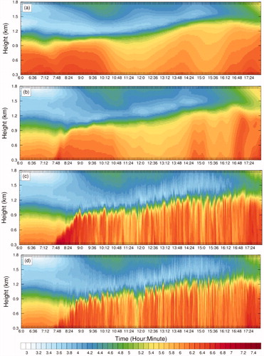
Changing to turbulence-permitting mode, namely switching-off the turbulence parameterization and switching-on the 3 D treatment of turbulence in the 300 m domain (panel c), the situation changed. Now, a clear transition from the nighttime stable to the daytime convective boundary layer became visible with the development of moist eddies growing in size over time with the increase of solar irradiance and therefore the heating of the ground. The boundary layer height during day was similar to the parameterized solution, but the downward mixing of dry air and upward mixing of moist air by turbulent eddies was clearly seen, leading to turbulent fluctuations of the boundary layer height, indicating that the LES-mode works reasonably well at that relatively coarse resolution. At a resolution of 100 m (panel d), the simulated structure was close to the 300 m representation, but even finer turbulent structures were resolved and a stronger variability during the day was seen. The entrainment processes were more pronounced.

To investigate whether differences in the land cover caused variations in the evolution of the CBL, time-height cross sections of the water vapor mixing ratio over different land covers are shown in Fig. 10 from the simulation with 100 m resolution in the same way as in Fig. 9. We excluded the lower resolution simulations, since the more inaccurate representation of the land surface makes it difficult to draw conclusions, especially when comparing the simulations with observations. We focused on the land cover classes cropland, urban, barren/sparsely vegetated and forest. The location of the profiles are marked by the letters C, U, B and F in the top panel of Fig. 5. The locations are away from the domain boundaries so that the development of turbulence was not influenced by the domain boundary.

Fig. 10. Evolution of the boundary layer over different land cover classes as seen in time-height cross sections of simulated water vapor mixing ratio (g/kg). From (a) to (d), the underlying land cover classes are cropland, urban, barren/sparsely vegetated and forest. Results are shown from the innermost 100 m domain.

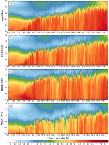
Over cropland and urban land covers (panels a and b), the simulations of the morning transition were similar. Nevertheless, slight differences occurred. The boundary layer growth during the morning transition was faster over urban areas compared to cropland but the gradual increase in PBL height during the day was similarly represented. Over the barren or sparsely vegetated surface (panel c), the boundary layer grew quickly to the final height in contrast to cropland and urban land cover types and remained, apart from the turbulent fluctuations, constant during day. Since the selected point is in the brown coal pit Hambach 200 to 300 m below the surroundings, this explains the deeper boundary layer. Over the forest point (panel d), the development was different. The boundary layer height remained smaller during the day and the ‘eddy structure’ appeared dissimilar to that of the other investigated land cover types.

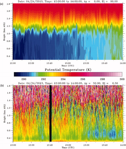
For comparisons with lidar data, we focused on the time period 12 to 14 UTC, 24 April 2013 since the PBL was well developed and the boundary layer height was, apart from turbulence-induced undulations, relatively constant. Figure 11 compares the simulated time-height cross section of potential temperature θ with the corresponding observation of the TRRL. Both data sets were interpolated to a time step of 10 s. An almost constant value of the simulated potential temperature with height illustrated the well-mixed convective boundary layer in the WRF-LES simulation. More internal structure and an on-average higher temperature was observed by the lidar. Especially in the first half of the time period, the simulated boundary layer was clearly colder than observed.

Fig. 11. Time-height cross sections of the lowest 1.8 km of the atmosphere of potential temperature (K). WRF simulation with 100 m resolution (a) and TRRL observation (b) for the period 12 to 14 UTC, 24 April 2013.

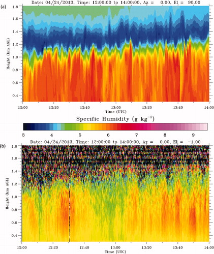
Figure 12 compares the simulated time-height cross section of specific humidity with the corresponding observation from the Hohenheim WVDIAL system. The single turbulent eddies transporting moist air upwards and entraining drier air down into the boundary layer explain the temporal undulation of the boundary layer height. The simulated eddies reached a vertical extent corresponding to the PBL height and had temporal scales in the range of minutes, corresponding to the values expected in the daytime convective boundary layer (e.g. Behrendt et al., 2015; Muppa et al., 2016; Wulfmeyer et al., 2016). Compared to the lidar observation, as for the potential temperature, less internal turbulent structure was simulated in the boundary layer. Furthermore, the entrainment of drier air into the boundary layer was clearly stronger and broader in the lidar observation. For instance, a substantial drying occurred between 12:40 and 13:10 UTC, while this was not simulated by the model. Although the variability in the simulation and the observation was comparable, the model simulated a moister boundary layer than observed.

Fig. 12. Time-height cross sections of the lowest 1.8 km of the atmosphere of specific humidity (g/kg). WRF simulation with 100 m resolution (a) and WVDIAL observation (b) for the period 12 to 14 UTC, 24 April 2013.

3.3. Turbulence statistics

Due to the stochastic nature of turbulence, an exact match between observations and model simulation is not possible - even if the model would be initialized by a re-assimilation of observations. In the following, we focus on the capability of the model to represent the boundary layer turbulence in a statistical sense. Therefore, point statistics of simulated potential temperature and specific humidity were calculated for the period 12 to 14 UTC, 24 April 2013 and compared with corresponding observations from the Hohenheim lidar systems, as explained in Section 2.6. Again, the results of the four different resolutions were included to investigate the benefit of the higher resolution.

Figure 13 compares temporally averaged vertical profiles (1st moment) of potential temperature (panel a) and specific humidity (panel b) of the model with lidar observations for the well-developed boundary layer in the time period 12 to 14 UTC, April 24 2013. The boundary layer heights, estimated from the backscatter data of the DIAL system, a radiosonde ascent and the different model resolutions are compared in Table 4. The simulated PBL height was lower by about 200 m than the observation but consistent within 100 m in the different model resolutions. In terms of potential temperature, all model resolutions showed a well-mixed boundary layer and through the whole profile, the temperatures were simulated within 1 K, again stressing that the simulations with turbulence parameterization are capable to capture the temperature structure. As mentioned for the time-height cross sections above, no internal structure was simulated. The average temperature of all simulations was lower by about 1 K throughout the boundary layer. Due to the observed internal structure in the entrainment layer and the higher boundary layer top, the simulated temperatures were higher in the height range between 1150 and 1400 m and lower above. Despite this, throughout the whole profile, the simulated temperature did not deviate more than 1 K from the observations.

Fig. 13. Comparison of observed and simulated mean vertical profiles of potential temperature (K) (a) and specific humidity (g/kg) (b) for the period 12 to 14 UTC, 24 April 2013.

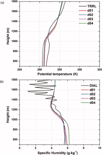
Table 4. Average PBL height for the observations and the different model resolutions during the period 12 to 14 UTC, 24 April 2013.

Platform	PBL height [m]
Radiosonde	1416
Lidar (Backscatter signal, WVDIAL)	1395
WRF D01 (2700 m resolution)	1135
WRF D02 (900 m resolution)	1179
WRF D03 (300 m resolution)	1136
WRF D04 (100 m resolution)	1150

In terms of specific humidity, the behavior of the simulations with and without turbulence parameterization was different. The profiles of the simulations with parameterization were close to the observed profile, but the specific humidity decreased with height, illustrating that the well-mixed nature of the boundary layer was not simulated. For the turbulence-permitting simulations, the specific humidity was about 0.7 g/kg higher than observed, but constant through the lowest 900 m, indicating that the boundary layer was well mixed. The larger values as compared to the lower resolution simulations illustrated the stronger vertical mixing in TP mode since largest values of moisture are expected at the surface. A constant specific humidity in the boundary layer is more in accordance to the expected profile in a well-mixed boundary layer (e.g. Xu et al., 2018). Due to the lower boundary layer height in the simulations, the strong drop of specific humidity with height started at lower altitudes than observed. In the lidar observations, the humidity was more gradually reduced, presumably due to the internal structure in the entrainment layer that was also seen in the temperature profile.

Vertical profiles of the variances (2nd moment) of potential temperature and specific humidity for the same time period are presented in Fig. 14. The variances highlight the regions where the temporal differences of the fields are largest. The variance profiles of the two lower resolution domains were not included into the comparison since their absolute values were, as expected, at least two orders of magnitude smaller since the internal structure of the boundary layer cannot be captured when a turbulence scheme is applied (not shown). For potential temperature (panel a), the model captured the general variance structure in the boundary layer. However, lower variances were simulated throughout the boundary layer. Up to a height of 1000 m, the lidar observed variances between 0.15 and 0.2 K², whereas it was almost zero in the simulations. The peak of largest variance was correctly located at the top of the boundary layer where the variance is largest due to alternating upward and downward mixing and the strongest gradient of the potential temperature. Since the simulated PBL height was located at approx. 1140 m (see Table 5) compared to a value of 1400 m estimated from backscatter data of the WVDIAL, the variance peaks occurred at different heights. As for the lower levels, the absolute values of the simulated variances in the peaks were lower than observed, indicating underestimated turbulence in the simulations. Comparing the two model resolutions indicates that the 100 m resolution can resolve more of the observed variability.

Fig. 14. Comparison of observed and simulated vertical profiles of temporal variances of potential temperature (K²) (a) and specific humidity (g²/kg²) (b) for the period 12 to 14 UTC, 24 April 2013.

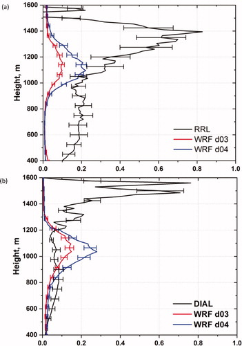
In terms of specific humidity variance (Fig. 14, panel b), the simulated and observed profiles were closer to each other up to a height of 800 m. Although the simulated variability was slightly less than observed, the values are within 0.1 g²/kg². This changed in the upper part of the boundary layer and above. Whereas the model simulations placed the peaks of the variance profiles below the boundary layer height into the entrainment layer (approx. 1050 m), it was located above the boundary layer top (approx. 1450 m) in the WVDIAL observation. As for the potential temperature, the absolute values of the simulated variance were lower than observed with higher values in the 100 m resolution domain, but the peak height region coincided in the simulations.

4. Discussion

The simulation of atmospheric boundary layer flows is a challenging problem since it involves the interaction of microscale three-dimensional turbulence with quasi two-dimensional synoptic and mesoscale structures (e.g. Muñoz-Esparza et al., 2015). Recent advances in computational capabilities allow an online coupling of mesoscale to LES simulations for real case studies. By doing this, high-resolution flow features are simulated while still considering the large-scale characteristics of the flow and the realistic forcing of the large-scale meteorological analysis (Mazzaro et al., 2017).

Problems occur when nesting an LES model into a mesoscale model (e.g. Moeng et al., 2007). Since the turbulent exchange coefficients are parameterized when using a PBL scheme, the flow is per definition laminar in the mesoscale domain and the turbulence has to develop out of nothing in the higher-resolution turbulence-permitting nest. Since the model physics is the same across the domains, apart from the switched-off turbulence scheme in the inner two domains, the problem is reduced. Nevertheless, time and space toward the upstream lateral boundaries are needed to spin-up turbulence.

The presented horizontal distributions of water vapor mixing ratio and vertical velocity (Figs. 7 and 8) show that the TP simulation was capable of representing the diurnal evolution of the boundary layer under fair weather conditions. During the morning, larger vertical velocities only occurred in regions with orographic forcing. In large parts of the domain, roll-type structures developed, typical for boundary layers with weak turbulence (Weckwerth et al., 1999).

With increasing surface heating, the circulation more and more broke apart into turbulent eddies. In some regions, coherent structures developed, so that turbulence evolved anisotropically. This is caused by orographic forcing and the heterogeneity of the underlying land surface. In regions where one land cover type prevails and the orography is relatively homogenous, the turbulence developed isotropically.

Strongest vertical mixing of moisture occurred in the southeastern corner of the domain. A closer look to the surface variables revealed that this is the consequence of (1) suppressed near surface wind to the lee of the mountains, (2) lower elevation and therefore higher near surface temperatures and (3) larger amounts of near surface moisture. When turbulent eddies were triggered over the mountains in the southern part of the domain and transported to the east, the turbulence was enhanced over the warmer surface and at the same time not disturbed by surface winds. This triggered a faster vertical transport of moisture in this region. A later change of the wind direction from southwesterly to westerly direction advected drier and more stable air into the southeastern corner of the domain in the afternoon (not shown), explaining the weakening of turbulence and the reduction of the upward moisture flux.

The narrow region of weak turbulence along the windward boundaries is promising since it indicates that the transition from the 300 m domain to the 100 m domain was restricted to a narrow belt along the inflow boundaries. This suggests that the applied methodology of downscaling the real synoptic situation from mesoscale to turbulence-permitting resolutions is a valid approach. This was true, despite the selected grid ratio between the domains being relatively large (a factor of 3) as compared to, e.g., the ICON LES model (Dipankar et al., 2015; Heinze et al., 2017) where a factor of two is used between the nests.

One should keep in mind that the area influenced by the outer domain depends on the large-scale synoptic situation and the stratification of the atmosphere. We focused on a fair weather day with weak large-scale forcing. Nevertheless, in the morning with weak turbulence, the influence of the coarser domain extended further into the finer-scale domain. Therefore, it is important to adjust the inner domain to the needs of the analysis and, e.g., place the lateral boundary far away from the region of interest when the onset of turbulence in the morning is the target of the analysis, as done in this study.

Mazzaro et al. (2017) investigated the capability of such a nesting strategy. With an idealized setup, they examined whether unrealistic lateral forcing of coarser scale simulations negatively influences the high-resolution LES simulation. They compared simulations using a turbulence parameterization as driving model with stand-alone LES simulations and demonstrated, that the assumption of horizontal homogeneity in the grid box in the turbulence parameterization results in an overestimation of total TKE and an underestimation of the Reynolds stress. Nevertheless, they confirmed that the nested high-resolution LES simulation could recover from the unrealistic conditions as long as the domain setup gives enough room for the development of turbulence. This was confirmed by our configuration tests.

Comparison of time-height cross sections of the water vapor mixing ratio simulated with the four different resolutions revealed that the expected vertical and temporal distribution in the boundary layer was only realistically represented when the model was operated in TP mode. The PBL scheme ensured that the height of the boundary layer and its coarse temporal evolution were realistically represented. However, the expected internal structure could not be captured. During the sensitivity tests to find the optimal model configuration, simulations with 300 m horizontal resolution with and without the turbulence scheme were compared (not shown). Although the 300 m simulation with turbulence scheme starts to simulate first eddies, the internal structure as well as the morning transition from the stable nighttime to the daytime convective boundary layer was more realistically represented in TP mode.

The limitation of one-dimensional turbulence schemes in capturing the internal structure of the boundary layer was also discussed by Muñoz-Esparza et al. (2016). They proposed that it is caused by the assumption of horizontal homogeneity in the grid cell, which becomes less and less true at increasingly fine grid scales. They also demonstrated that the schemes are capable of representing the coarse vertical structure of the boundary layer and concluded that its representation in mesoscale simulations would benefit from three-dimensional PBL schemes (e.g. Jiménez and Kosovic, 2016) accounting for all components of the Reynolds stress tensor. The benefit would be largest when the system is applied in orographic terrain, as done in our case. Nested turbulence-permitting or LES simulations would then further benefit from the more realistic forcing.

To investigate the influence of different land cover types on the evolution of the boundary layer, time-height cross sections were derived over different land cover classes. Coarser resolution simulations were not included since at coarser resolution more than just one land cover class in the grid box occur and the applied NOAH-MP land surface model only considers the dominant land cover category. Figure 10 shows that the boundary layer evolution over different land cover classes was similar, but with fine scale differences still occurring. The daytime rise of the boundary layer height was linear over the urban surface because of the expected constant surface temperature rise due to less moisture available for evaporation and urban structures quickly storing heat. The importance of urban surfaces on the representation of the evolution of the boundary layer above was also investigated by Song and Wang (2015) and Song et al. (2018). Furthermore, the variability of the boundary layer is larger in urban areas due to the larger roughness. Over cropland, the PBL height remained constant during the morning and quickly rose later to similar heights as over urban land cover. The reason for this behavior may be that cropland cools stronger during night, so that the daytime growth of the boundary layer starts later as compared to the urban boundary layer. Furthermore, evaporation from the moister cropland surface in the morning reduced the surface temperature rise. Over barren/sparsely vegetated surface, the PBL height rose quickly to its final height and remained almost constant during the rest of the simulation. This could be caused by the strong heating of the barren land surface as compared to a vegetated one and also explains the larger temporal variability of water vapor mixing ratio as compared to, e.g., cropland. The total height of the boundary layer was higher than over cropland and urban surfaces since the selected grid cell is in the brown coal pit 200 to 300 m below the surrounding landscape. Over forest, the simulated lower PBL height was expected since the moister surface and associated larger latent heat flux compared to cropland and urban surfaces reduces the surface temperature, resulting in lower sensible heat fluxes, and a lower boundary layer height. Furthermore, the temporal structure of the eddies differs and the overall variability of water vapor is larger due to the greater roughness in combination with the lower surface temperature.

Detailed comparisons of the simulated boundary layer with lidar observations demonstrated that the WRF TP simulations represented a well-mixed CBL with the potential temperature remaining constant over the height of the boundary layer. However, the corresponding profile from the TRRL was not constant, indicating vertical internal structure that could not be resolved by the simulations. This is not surprising since the lidar observed a much smaller area of less than a square meter, whereas the model grid mesh was 100 × 100 m. Furthermore, the simulated temperature in the boundary layer was lower than observed between 12:00 and 13:20 UTC. After 13:20 UTC, a cooling was indicated by lidar and the observed and simulated temperatures were similar. Comparison of the simulated and observed surface temperature in the grid cell of the lidar site revealed that the modeled surface temperature was 2 K lower than observed at the beginning of the selected time period. This led to lower sensible heat fluxes and therefore a lower PBL height (see Table 5). In addition, it explains the lower temperatures throughout the boundary layer in the simulation due to the weaker transport of heat to higher levels.

Comparison of specific humidity again revealed a lower variability in the simulation caused by the coarser mesh. Nevertheless, the resolved turbulent eddies resulted in a realistic undulation of the boundary layer height with time. With heights up to the CBL top and durations up to a few minutes, the temporal and spatial scales of the eddies corresponded to the values expected for a convective boundary layer (e.g. Wulfmeyer et al., 2016). However, an exact match of observation and simulation is not possible due to the stochastic nature of turbulence, even with finer and finer grids or improved initialization of the simulations with data assimilation.

The averaged profiles of potential temperature (Fig. 13a) of all four model resolutions were close to each other. They were simulated within 0.5 degrees up to 1800 m a.s.l., confirming that the temperature structure of the boundary layer was represented even in simulations with turbulence parameterization. The observed vertical profile from the TRRL was not constant with height, indicating vertical internal structure in the boundary layer that could not be captured even by the fine-scale 100 m grid. Furthermore, the observed profile was approximately 0.5 K warmer throughout the boundary layer caused by a lower surface temperature in the simulation. The higher observed boundary layer height explained the crossings of the modelled and observed profiles and the increase of observed potential temperature at higher levels.

The comparison of averaged specific humidity profiles for the different model resolutions showed that the two coarser resolutions with parameterized turbulence simulated an approximately 0.5 g/kg drier boundary layer compared to the two higher-resolution domains in TP mode. The high-resolution profiles showed the well-mixed nature of the boundary layer with constant specific humidity, while, the specific humidity slightly dropped with height in the coarser simulations, indicating that the turbulence parameterization could not reproduce the well-mixed nature of the boundary layer for water vapor. Comparison of the lowest levels in the time-height cross sections (Figs. 11 and 12) showed that the temperature was lower and the specific humidity was higher in the simulations as compared to the observations, explaining the differences found at higher levels in the PBL.

Comparing with lidar, the coarser simulations were closer to the observations in terms of their absolute values as compared to the turbulence-permitting simulations. This could be explained by the moister near surface air in the turbulence-permitting simulations combined with stronger turbulent mixing equally distributing larger amounts of moisture in the boundary layer. The observed larger internal structure and the higher boundary layer top as compared to the simulations explain the differences between the observed and simulated profiles.

Simulated and observed variance profiles of potential temperature and specific humidity were compared in Fig. 14. The turbulence-permitting simulations with 300 m and 100 m showed almost no variance in potential temperature throughout the boundary layer, whereas an almost constant variance of 0.2 K² was observed by the TRRL. This indicates that even a resolution as high as 100 m could not fully capture the internal variability of temperature in the boundary layer. The peak at the top of the boundary layer with largest temperature variations was correctly located in the simulations (see e.g. Turner et al., 2014), but the absolute values were lower and the simulated height of the boundary layer was lower than observed. Larger variance values in the higher 100 m resolution indicate that more variability was captured with higher resolution. An even higher resolution than 100 m may therefore lead to an even closer match between the simulated and observed profiles.

The simulated variances of specific humidity were also lower than observed, but up to a height of 900 m, the differences to the WVDIAL were within 0.1 g²/kg². The simulations placed the peak of the moisture variance below the boundary layer height of approx. 1140 m (see Table 4) and the 100 m simulation resolved more variance than the one with 300 m resolution. The WVDIAL observed the peak above the boundary layer top of 1395 m. The WVDIAL wavelength was chosen to investigate the humidity structure in the convective boundary layer, explaining a large part of the variability observed further above.

The result that the model places the maximum below the boundary level height into the entrainment layer while the observed peak is located above the boundary layer top indicates that the simulations might not capture the processes around the boundary layer top correctly. This may be caused by the coarser vertical and horizontal resolutions and/or by a too strong entrainment at the top of the boundary layer in the WRF simulations. Heinze et al. (2017) compared simulations with the ICON-LES model with lidar data and their moisture variance profiles showed the same characteristics, indicating that models with resolutions of 100 m face problems in representing the processes at the top of the boundary layer correctly. It will be investigated in upcoming studies whether an even higher horizontal and vertical resolution can solve some of the mentioned issues. Although differences in detail occurred, the comparisons showed that the statistical evolution of turbulence was represented by turbulence-permitting WRF simulations as compared to lidar observations and that the selected approach can be applied for turbulence research in real case simulations.

5. Summary and conclusions

A multi-nested setup of WRF version 3.7.1 was successfully applied to investigate its performance in representing turbulence and the spatial and temporal evolution of the boundary layer. The model system was setup in a 4-nest configuration with a grid ratio of three between the nests. The outermost domain, driven by the ECMWF analysis had a horizontal resolution of 2700 m, with 900 m, 300 m and 100 m nests embedded into the coarsest domain. The atmosphere up to 50 hPa was discretized into 121 vertical levels to properly represent the temporal and spatial details in the turbulence-permitting simulations. The system used a carefully selected set of physical options and ran for a clear sky day during the HOPE experiment in Germany in spring 2013. The investigation of the evolution of the simulated convective boundary layer was complemented by comparisons of turbulence statistics with lidar observations.

The results showed that the selected modeling approach was capable to represent the expected evolution of the boundary layer and the observed turbulence statistics with differences occurring in the details. To conclude the paper, the scientific questions posed in the introduction are finally answered.

What is the optimal setup of the model chain for the application in the daytime convective boundary layer?

To find the best possible configuration for the simulation, a series of sensitivity tests was carried out. The spatial and temporal developments of turbulence in the simulations strongly depend on the selected setup. The most important configuration characteristics are the number of vertical levels, the applied domain sizes, and whether the turbulence parameterization is applied or switched-off in the 300 m domain. The number of vertical levels was finally set to 121 up to 50 hPa with more than 30 levels in the lowest 1500 m of the atmosphere. Furthermore, the turbulence parameterization was already switched-off in the 300 m domain. This forcing of a turbulence-permitting domain with a coarser turbulence-permitting domain lead to a faster adjustment between the two nests and therefore a more realistic development of turbulence in the innermost domain. This corresponds to findings of Mirocha et al (2010) who found similar results for idealized WRF-LES setups. Due to the application of the NOAHMP land surface model and higher resolution data sets of orography, land use and soil characteristics, the land surface and its interaction with the lower atmosphere was more realistically captured in our simulations compared to earlier simulations that did not apply those data sets. Finally, the domain size of the two inner domains was increased from 301 × 301 to 502 × 502 grid cells to give the turbulence more space to develop to ensure that it is fully evolved in the region of interest in the domain.

In this investigation, no obvious problems caused by the parameterizations were found, as e.g. a reduction of the size of the meteorological phenomenon with the application of a finer model grid. However, more detailed sensitivity studies comparing simulations and observations are necessary to finally judge the scalability of the model physics for turbulence-permitting simulations. Such studies are possible using the comprehensive observational data set collected during the LAFE campaign conducted at the ARM site in Oklahoma in August 2017 (Wulfmeyer et al., 2018).

Since parameterization research and development continues steadily, more ‘scale-aware’ parameterizations can be included in future simulations. The recently released model version 4.1 of WRF now contains two scale-aware PBL schemes and one scale-aware cloud microphysics scheme. It is expected that its implementation will improve the mesoscale forcing for nested turbulence-permitting and LES domains.

What are the general advantages of this multi-nested approach as compared to high-resolution mesoscale and/or idealized LES simulations? Is the gray zone better represented using this approach?

Both mesoscale and idealized LES simulations cannot be applied for answering the scientific questions posed in this manuscript. Due to the turbulence parameterization in mesoscale simulations, the development of turbulent eddies responsible for the vertical exchange of heat and moisture in the boundary layer, are not simulated. A coarser resolution is also associated with coarser representation of the lower boundary, weakening the comparability with state-of-the-art observations in highly heterogeneous landscapes. Idealized LES simulations with periodic boundary conditions are excellent tools to investigate the characteristics of turbulence, but they do not take into account that a heterogeneous landscape structure greatly influences the temporal and spatial evolution of turbulence as well as energy and water exchanges between the land surface and the atmosphere (e.g. Moeng et al., 2007; Zhu, 2008a, 2008b; Muñoz-Esparza et al., 2017). Such influences were demonstrated in our simulations

The introduced multi-nested approach allows a seamless integration of turbulence-permitting and even LES domains into mesoscale simulations. Driven by an accurate meteorological analysis, including sophisticated data sets to initialize the lower boundary, and selecting a nested configuration that gives the turbulence enough time and space to develop, the system is capable of reproducing the spatial and temporal evolution of the convective boundary layer for real cases. In case of WRF, this is done within the same model framework. The benefits of using consistent physics across scales cannot be overestimated since the model balance during nesting is disturbed as little as possible (e.g. Palmer et al., 2008; Martin et al., 2010).

Process understanding in the boundary layer and of LA exchange are important applications of the system in future applications. Furthermore, the comparison with sophisticated observations collected during field campaigns allows the verification, validation and even the improvement of existing parameterizations or the development of new ones.

How is the temporal and spatial evolution of the boundary layer represented by the different resolutions in the applied multi-scale approach?

The analysis showed that the coarse structure of the evolving convective boundary layer can be represented with the two outer domains applying a PBL scheme. The height of the boundary layer, its growth and the coarse temporal variation of moisture during day were captured. Some more detail, e.g., an indication of the morning transition was simulated with 900 m resolution, but still no details about the internal structure of the boundary layer and its temporal development were seen. In the higher-resolution turbulence-permitting simulations, the fine-scale temporal evolution of the boundary layer including the morning transition from the nighttime stable to the daytime convective boundary layer was simulated realistically. Furthermore, the turbulent eddies were captured and their spatial and temporal scales were in the range expected from a well-developed convective boundary layer. A comparison of 300 m simulations with and without the turbulence parameterization (not shown) revealed a more realistic performance without the use of a turbulence scheme.

Since the horizontal resolution of the simulation determines the resolution of the underlying land cover description and no sub-scale description is available in the applied NOAH-MP land surface scheme (Tile approach), one dominant land cover class is available as lower boundary of each grid cell. Furthermore, the underlying orography is represented better and better with increasing resolution (see Fig. 3). Therefore, it is expected that a more realistic description of the land cover and the orography in the domain at higher resolution also improves the LA exchange in the simulation. The time-height cross sections (Fig. 10) showed similar developments with differences occurring in details that can be explained by the different surface characteristics. However, more detailed comparisons with flux measurements from Eddy-Covariance stations and flux profiles derived from lidar data are necessary to further identify the processes simulated by the turbulence-permitting simulations over realistic land surface conditions. To do this, the LAFE campaign (Wulfmeyer et al., 2018) provides excellent data sets.

Is the statistical evolution of turbulence realistically represented by the model? What is the benefit of an increase in resolution for the representation of turbulence statistics?

We calculated the turbulence statistics following Lenschow et al. (2000) and Wulfmeyer et al. (2016) for all four model resolutions from time series output done in model resolution. Even the simulations with 2700 m and 900 m with applied YSU turbulence parameterization were able to simulate the expected averaged profiles of the specific humidity and potential temperature. This is not surprising, since turbulence parameterizations are usually tuned to represent such profiles correctly. In representing the second order moment, the variance, differences between the simulations became visible. Whereas the expected vertical profile of the variance could not be represented at all by the YSU turbulence parameterization, they were reasonably captured in the turbulence-permitting simulations. Comparing the two turbulence-permitting resolutions, the higher resolved 100 m domain better represented the variance profile of potential temperature compared with lidar observations, illustrating that at least a horizontal resolution of 100 m and a vertical resolution of 50 m is necessary to capture the profiles. The total variance of potential temperature was still underestimated in the 100 m domain, so that future studies should include simulations with even higher horizontal and vertical resolutions to elaborate whether the representation of the simulated higher order moments can be further improved. The variance of specific humidity was well represented by the turbulence-permitting simulations up to a height of 900 m. In the entrainment layer above, the simulated variance peak was simulated below the boundary layer top, whereas it was observed above the PBL top, indicating that the model cannot correctly capture the observed processes around the top of the boundary layer. Here, an even higher vertical resolution may contribute to an improved process representation.

The promising results of the study suggest the multi-nested system for different further applications. It will be applied to accompany other measurement campaigns for selected case studies. The simulations complement to the observations of the lidar systems and improve the capability to investigate the 3 D and 4 D structure of the boundary layer by providing its full 4-dimensional evolution. Detailed case studies for the evolution of selected meteorological processes in the boundary layer as well as the detailed structure of larger-scale processes (e.g. high-impact weather events) will be performed to increase their process understanding, Furthermore, the validation and improvement of parameterizations is possible from a process point of view.

Since the number of applications of WRF at very high resolution is constantly growing, improvements of the system for such applications may be expected in future releases of the model system. This is true for the numerical core of the model (e.g. Xiao et al., 2015) as well as the physics schemes. Room for optimization also exists in the representation of sub-filter scale turbulence. Approaches that are more sophisticated compared to the applied NBA method (Kosovic, 1997), namely the Lagrangian-Averaged Scale-Dependent (LASD; Bou-Zeid et al., 2005) method and the Dynamic Reconstruction Model (DRM; Chow et al., 2005) were successfully tested with WRF (Mirocha et al., 2014), but are not part of the release version. Another possibility to accelerate the development of turbulence at the mesoscale – LES boundary is the use of so-called perturbation models (e.g. Muñoz-Esparza et al., 2014). They additionally perturb the potential temperature field along the inflow boundaries to trigger turbulence and allow the application of larger grid ratios between the domains to jump over the grey zone from one domain to the next (e.g. Muñoz-Esparza et al., 2017). Last, but not least a further increase of the horizontal and vertical resolutions in the innermost domain is expected to improve the representation of the boundary layer processes in the simulations, but at the cost of largely increased computational demands.

This nested WRF-NOAHMP configuration will be used for a variety of applications. These include (1) a comparison of turbulence parameterizations with observations from the LAFE campaign, the Land Atmosphere Feedback Observatory (LAFO) in Hohenheim as well as other previous and future field campaigns. For this purpose, all relevant parameters and variables will be extracted from the convection-permitting model runs, e.g., for comparing parameterized with observed flux profiles. (2) A thorough comparison of turbulent variables derived by LES with observations. This is now possible using the LAFE synergy based on lidar systems with turbulence resolution. (3) The test and the improvement of turbulence parameterizations by the combination of the results of (1) and (2). These activities will be imbedded in international projects such as the WCRP Global Land Atmosphere System Study (GLASS) and its Local Coupling (LoCo) subproject.

Acknowledgements

ECMWF is acknowledged for the provision of the analysis data applied for the initial and lateral forcing of the outermost model domain. The WRF simulations were done on the systems ‘ForHLR I’ and ‘bwUniCluster’, part of the high performance computing facilities of the state of Baden Wuerttemberg. The MSG satellite composites were provided by the NERC satellite receiving station of the Dundee University, Scotland. The high-resolution SRTM orography data was retrieved from the CIAT-CSI SRTM webpage (http://srtm.csi.cgiar.org) and the CORINE land cover data set was downloaded from the Copernicus Land Monitoring Service webpage (https://land.copernicus.eu/pan-europe/corine-land-cover). Finally, the WRF developer team and the contributing community are thanked for their tireless efforts to improve the model system. The lidar data used in this work were recorded during the HOPE campaign, embedded in the HD(CP)² project, funded by the Federal Ministry of Education and Research in Germany.

Disclosure statement

No potential conflict of interest was reported by the authors.

Additional information

Funding

The lidar data used in this work were recorded during the HOPE campaign, embedded in the HD(CP)² project, funded by the Federal Ministry of Education and Research in Germany.

Notes

1 IHOP: International H₂O Project

2 LITFASS: Lindenberg Inhomogeneous Terrain – Fluxes between Atmosphere and Surface: a Long-term Study

3 COPS: Convective and Orographically-induced Precipitation Study

4 HOPE: High Definition Clouds and Precipitation for advancing Climate Predictions - HD(CP)² - Observation Prototype Experiment

5 SABLE: Surface-Atmospheric Boundary Layer Exchange

6 LAFE: Land - Atmosphere Feedback Experiment

References

- Abdolghafoorian, A., Farhadi, L., Bateni, S. M., Margulis, S. and Xu, T. 2017. Characterizing the effect of vegetation dynamics on the bulk heat transfer coefficient to improve variational estimation of surface turbulent fluxes. J. Hydrometeor. 18, 321–333. doi:10.1175/JHM-D-16-0097.1
- Balzarini, A., Angelini, F., Ferrero, L., Moscatelli, M., Perrone, M. G. and co-authors. 2014. Sensitivity analysis of PBL schemes by comparing WRF model and experimental data. Geosci. Model Dev. Discuss. 7, 6133–6171. doi:10.5194/gmdd-7-6133-2014
- Bauer, H.-S., Weusthoff, T., Dorninger, M., Wulfmeyer, V., Schwitalla, T. and co-authors. 2011. Predictive skill of a subset of the D-PHASE multi-model ensemble in the COPS region. COPS special issue of the Q. Q. J. R. Meteorol. Soc. 137, 287–305. doi:10.1002/qj.715
- Behrendt, A., Wulfmeyer, V., Hammann, E., Muppa, S. K. and Pal, S. 2015. Profiles of second to fourth-order moments of turbulent temperature fluctuations in the convective boundary layer. First measurements with rotational Raman lidar. Atmos. Chem. Phys. 15, 5485–5500. doi:10.5194/acp-15-5485-2015
- Beyrich, F., Leps, J.-P., Mauder, M., Bange, J., Foken, T. and co-authors. 2006. Area-averaged surface fluxes over the litfass region based on eddy-covariance measurements. Bound.-Lay. Meteorol. 121, 33–65. doi:10.1007/s10546-006-9052-x
- Bou-Zeid, E., Meneveau, C. and Parlange, M. B. 2005. A scale-dependent Lagrangian dynamic model for large eddy simulation of complex turbulent flows. Phys. Fluids 17, 025105. doi:10.1063/1.1839152
- Buettner, G. 1998. The European CORINE land cover database. In: Proceedings of the ISPRS Commission VII Symposium. Budapest, September 1–4, pp. 633–638.
- Buettner, G., Ferrare, G. and Jaffrain, G. 2002. CORINE land cover update 2000 – technical guidelines. European Environment Agency. Technical report 89. Online at: http://reports.eea.europe.eu/technical_report_2002.89/en.
- Cai, X., Yang, Z.-L., Xia, Y., Huang, M., Wei, H. and co-authors. 2014. Assessment of simulated water balance from Noah, Noah-MP, CLM, and VIC over CONUS using the NLDAS testbed. J. Geophys. Res. Atmos. 119, 13,751–13770. doi:10.1002/2014JD022113
- Chen, Q. and Tong, C. 2006. Investigation of three subgrid-scale stress and its production rate in a convective atmospheric boundary layer using measurement data. J. Fluid Mech. 547, 65–104. doi:10.1017/S0022112005007196
- Chlond, A., Müller, F. and Sednev, I. 2004. Numerical simulation of the diurnal cycle of marine stratocumulus during FIRE - A LES and SCM modelling study. Q. J. R. Meteorol. Soc. 130, 3297–3321. doi:10.1256/qj.03.128
- Chlond, A. and Wolkau, A. 2000. Large-eddy simulation of a nocturnal stratocumulus-topped marine atmospheric boundary layer: An uncertainty analysis. Bound. Lay. Meteorol. 95, 31–55. doi:10.1023/A:1002438701638
- Chow, F. K., Street, R. L., Xue, M. and Ferziger, J. H. 2005. Explicit filtering and reconstruction turbulence modeling for large-eddy simulation of neutral boundary layer flow. J. Atmos. Sci. 62, 2058–2077. doi:10.1175/JAS3456.1
- Cohen, A. E., Cavallo, S. M., Coniglio, M. C. and Brooks, H. E. 2015. A review of planetary boundary layer parameterization schemes and their sensitivity in simulating southeastern U.S. cold season severe weather environments. Weather Forecast. 30, 591–612. doi:10.1175/WAF-D-14-00105.1
- Deardorff, J. W. 1974. Stratocumulus-capped mixed layers derived from a three-dimensional model. Bound.-Lay. Meteorol. 7, 199–226. doi:10.1007/BF00227913
- De Kauwe, M. G., Medlyn, B. E., Knauer, J. and Williams, C. A. 2017. Ideas and perspectives: How coupled is the vegetation to the boundary layer? Biogeosciences 14, 4435–4453. doi:10.5194/bg-14-4435-2017
- Di Girolamo, P., Cacciani, M., Summa, D., Scoccione, A., De Rosa, B. and co-authors. 2017. Characterization of boundary layer turbulent processes by the Raman lidar BASIL in the frame of HD(CP)2 observational prototype experiment. Atmos. Chem. Phys. 17, 745–767. doi:10.5194/acp-17-745-2017
- Dipankar, A., Stevens, B., Heinze, R., Moseley, C., Zängl, G. and co-authors. 2015. Large eddy simulation using the general circulation model ICON. J. Adv. Model. Earth Syst. 7, 963–986. doi:10.1002/2015MS000431
- Efstathiou, G. A., Beare, R. J., Osborne, S. and Lock, A. P. 2016. Grey zone simulations of the morning convective boundary layer development. J. Geophys. Res. Atmos. 121, 4769–4782. doi:10.1002/2016JD024860
- Farr, T. G., Rosen, P. A., Caro, E., Crippen, R., Duren, R. and co-authors. 2007. The shuttle radar topography mission. Rev. Geophys. 45, RG2004.
- Feng, Z., Leung, L. R., Houze, R. A., Jr., Hagos, S., Hardin, J. and co-authors. 2018. Structure and evolution of mesoscale convective systems: Sensitivity to cloud microphysics in convection-permitting simulations over the United States. J. Adv. Model. Earth Syst. 10, 1470–1494. doi:10.1029/2018MS001305
- Green, J. K., Konings, A. G., Alemohammad, S. H., Berry, J., Entekhabi, D. and co-authors. 2017. Regionally strong feedbacks between the atmosphere and terrestrial biosphere. Nat. Geosci. 10, 410–414. doi:10.1038/ngeo2957
- Hammann, E., Behrendt, A., Le Mounier, F. and Wulfmeyer, V. 2015. Temperature profiling of the atmospheric boundary layer with rotational Raman lidar during the HD(CP)2 observational prototype experiment. Atmos. Chem. Phys. 15, 2867–2881. doi:10.5194/acp-15-2867-2015
- Heinze, R., Dipankar, A., Carbajal Henken, C., Moseley, C., Sourdeval, O. and co-authors. 2017. Large-eddy simulations over Germany using ICON: A comprehensive evaluation. Q. J. R. Meteorol. Soc. 143, 69–100. doi:10.1002/qj.2947
- Heus, T., van Heerwaarden, C. C., Jonker, H. J. J., Pier Siebesma, A., Axelsen, S. and co-authors. 2010. Formulation of the Dutch atmospheric large-eddy-simulation (DALES) and overview of its application. Geosci. Model Dev. 3, 415–444. doi:10.5194/gmd-3-415-2010
- Hong, S.-Y., Noh, Y. and Dudhia, J. 2006. A new vertical diffusion package with an explicit treatment of entrainment processes. Mon. Weather Rev. 134, 2318–2341. doi:10.1175/MWR3199.1
- Hong, S.-Y., Park, H., Cheong, H.-B., Kim, J.-E. E., Koo, M.-S. and co-authors. 2013. The global/regional integrated model system (GRIMs). Asia-Pacific J. Atmos. Sci. 49, 219–243. doi:10.1007/s13143-013-0023-0
- Honnert, R., Masson, V. and Couvreux, F. 2011. A diagnostic for evaluating the representation of turbulence in atmospheric models at the kilometric scale. J. Atmos. Sci. 68, 3112–3131. doi:10.1175/JAS-D-11-061.1
- Honnert, R. and Masson, V. 2014. What is the smallest physically acceptable scale for 1D turbulence schemes? Front. Earth Sci. 2, 1–5.
- Huang, M., Gao, Z., Miao, S. and Chen, F. 2019. Sensitivity of urban boundary layer simulations to urban canopy models and PBL schemes in Beijing. Meteorol. Atmos. Phys. 131, 1235–1248. doi:10.1007/s00703-018-0634-1
- Iacono, M. J., Delamere, J. S., Mlawer, E. J., Shephard, M. W., Clough, S. A. and co-authors. 2008. Radiative forcing by long-lived greenhouse gases: Calculations with the AER radiative transfer models. J. Geophys. Res. 113, D13103. doi:10.1029/2008JD009944
- Jankov, I., Grasso, L. D., Sengupta, M., Neiman, P. J., Zupanski, D. and co-authors. 2011. An evaluation of five ARW-WRF microphysics schemes using synthetic GOES imagery for an atmospheric river event affecting the California coast. J. Hydrometeor. 12, 618–633. doi:10.1175/2010JHM1282.1
- Jarvis, A., Reuter, H., Nelson, A. and Guevara, E. 2008. Hole-filled seamless SRTM data v4, International Center for Tropical Agriculture (CIAT). Online at: http://srtm.csi.cigar.org
- Jiménez, P. A., Dudhia, J., González-Rouco, J. F., Navarro, J., Montávez, J. P. and co-authors. 2012. A revised scheme for the WRF surface layer formulation. Mon. Weather Rev. 140, 898–918. doi:10.1175/MWR-D-11-00056.1
- Jiménez, P. and Kosovic, B. 2016. Implementation and evaluation of a three dimensional PBL parameterization for simulations of the flow over complex terrain. In: 17th Annual WRF Users’ Workshop, National Center for Atmospheric Research, Boulder, Colorado.
- Kirkil, G., Mirocha, J., Bou-Zeid, E., Chow, F. K. and Kosović, B. 2012. Implementation and evaluation of dynamic subfilter-scale stress models for large-eddy simulation using WRF. Mon. Weather Rev. 140, 266–284. doi:10.1175/MWR-D-11-00037.1
- Kosovic, B. 1997. Subgrid-scale modeling for the large-eddy simulation of high Reynolds number boundary layers. J. Fluid Mech. 336, 151–182. doi:10.1017/S0022112096004697
- Lenschow, D. H., Wulfmeyer, V. and Senff, C. 2000. Measuring second-through fourth-order moments in noisy data. J. Atmos. Oceanic Technol. 17, 1330–1347. doi:10.1175/1520-0426(2000)017<1330:MSTFOM>2.0.CO;2
- Lilly, D. K. 1968. Models of cloud-topped mixed layers under a strong inversion. Q. J. R. Meteorol. Soc. 94, 292–309. doi:10.1002/qj.49709440106
- Lin, T. and Cheng, F. 2016. Impact of soil moisture initialization and soil texture on simulated land–atmosphere interaction in Taiwan. J. Hydrometeor. 17, 1337–1355. doi:10.1175/JHM-D-15-0024.1
- Macke, A., Seifert, P., Baars, H., Beekmans, C., Behrendt, A. and co-authors. 2017. The HD(CP)2 observational prototype experiment HOPE – An overview. Atmos. Chem. Phys. 17, 4887–4837. doi:10.5194/acp-17-4887-2017
- Maronga, B., Gryschka, M., Heinze, R., Hoffmann, F., Kanani-Sühring, F. and co-authors. 2015. The parallelized large-eddy simulation model (PALM) version 4.0 for atmospheric and oceanic flows: Model formulation, recent developments, and future perspectives. Geosci. Model Dev. 8, 2515–2551. doi:10.5194/gmd-8-2515-2015
- Martin, G. M., Milton, S. F., Senior, C. A., Brooks, M. E., Ineson, S. and co-authors. 2010. Analysis and reduction of systematic errors through a seamless approach to modeling weather and climate. J. Clim. 23, 5933–5957. doi:10.1175/2010JCLI3541.1
- Martínez, I. R. and Chaboureau, P. 2018. Precipitation and mesoscale convective systems: Explicit versus parameterized convection over northern Africa. Mon. Weather Rev. 146, 797–812. doi:10.1175/MWR-D-17-0202.1
- Mazzaro, L. J., Muñoz-Esparza, D., Lundquist, J. K. and Linn, R. R. 2017. Nested mesoscale-to-LES modeling of the atmospheric boundary layer in the presence of under-resolved convective structures. J. Adv. Model. Earth Syst. 9, 1795–1810. doi:10.1002/2017MS000912
- Milovac, J., Ingwersen, J. and Warrach-Sagi, K. 2014a. Soil texture forcing data for the whole world for the weather research and forecasting (WRF) model of the University of Hohenheim (UHOH) based on the harmonized world soil database (HWSD) at 30 arc-second horizontal resolution. World Data Center for Climate (WDCC). doi:10.1594/WDCC/WRF_NOAH_HWSD_world_TOP_SOILTYP.
- Milovac, J., Ingwersen, J. and Warrach-Sagi, K. 2014b. Top soil texture forcing data for the area of Germany for the Weather Research and Forecasting (WRF) model based on the Bodenübersichtskarte (BUK) at a scale of 1:1000000 (BUK1000) and provided by the University of Hohenheim (UHOH). World Data Center for Climate (WDCC). doi:10.1594/WDCC/WRF_NOAH_BUK_Ger_top_SOILTYP
- Milovac, J., Warrach-Sagi, K., Behrendt, A., Späth, F., Ingwersen, J. and co-authors. 2016. Investigation of PBL schemes combining the WRF model simulations with scanning water vapor differential absorption lidar measurements. J. Geophys. Res. Atmos. 121, 624–649. doi:10.1002/2015JD023927
- Mirocha, J., Kosovic, B. and Kirkil, G. 2014. Resolved turbulence characteristics in large-eddy simulations nested within mesoscale simulations using the weather research and forecasting model. Mon. Weather Rev. 142, 806–831. doi:10.1175/MWR-D-13-00064.1
- Mirocha, J., Lundquist, J. K. and Kosovic, B. 2010. Implementation of a non-linear subfilter turbulence stress model for large-eddy simulation in the advanced research WRF model. Mon. Weather Rev. 138, 4212–4228. doi:10.1175/2010MWR3286.1
- Moeng, C. H. 1984. A large-eddy-simulation model for the study of the planetary boundary layer turbulence. J. Atmos. Sci. 41, 2052–2062. doi:10.1175/1520-0469(1984)041<2052:ALESMF>2.0.CO;2
- Moeng, C. H., Dudhia, J., Klemp, J. and Sullivan, P. 2007. Examining two-way grid nesting for large eddy simulation of the PBL using the WRF model. Mon. Weather Rev. 135, 2295–2311. doi:10.1175/MWR3406.1
- Morrison, H., Thompson, G. and Tatarskii, V. 2009. Impact of cloud microphysics on the development of trailing stratiform precipitation in a simulated squall line: Comparison of one- and two-moment schemes. Mon. Weather Rev. 137, 991–1007. doi:10.1175/2008MWR2556.1
- Muñoz-Esparza, D., Kosovic, B., Mirocha, J. and van Beeck, J. 2014. Bridging the transition from mesoscale to microscale turbulence in numerical weather prediction models. Bound.-Lay. Meteorol. 153, 409–440. doi:10.1007/s10546-014-9956-9
- Muñoz-Esparza, D., Kosovic, B., van Beeck, J. and Mirocha, J. 2015. A stochastic perturbation method to generate inflow turbulence in large-eddy simulation models: Application to neutrally stratified atmospheric boundary layers. Phys. Fluids 27, 035102. doi:10.1063/1.4913572
- Muñoz-Esparza, D., Lundquist, J. K., Sauer, J. A., Kosović, B. and Linn, R. R. 2017. Coupled mesoscale-LES modeling of a diurnal cycle during the CWEX-13 field campaign: From weather to boundary-layer eddies. J. Adv. Model. Earth Syst. 9, 1572–1594. doi:10.1002/2017MS000960
- Muñoz-Esparza, D., Sauer, J. A., Linn, R. R. and Kosovic, B. 2016. Limitations of one-dimensional PBL parameterizations in reproducing mountain-wave flows. J. Atmos. Sci. 73, 2603–2614. doi:10.1175/JAS-D-15-0304.1
- Muppa, S. K., Behrendt, A., Späth, F., Wulfmeyer, V., Metzendorf, S. and co-authors. 2016. Turbulent humidity fluctuations in the convective boundary layer. Case studies using water vapor DIAL measurements. Bound.-Lay. Meteorol. 158, 43–66. doi:10.1007/s10546-015-0078-9
- Nakayama, H., Tamura, T. and Abe, S. 2008. LES on plume dispersion in the convective boundary layer capped by a temperature inversion. J. Fluid Sci. Technol. 3, 519–532. doi:10.1299/jfst.3.519
- Niu, G.-Y., Yang, Z.-L., Mitchell, K. E., Chen, F., Ek, M. B. and co-authors. 2011. The community Noah land surface model with multiparameterization (Noah-MP): Model description and evaluation with local-scale measurements. J. Geophys. Res. 116, D12109,
- Palmer, T. N., Doblas-Reyes, F. J., Weisheimer, A. and Rodwell, M. J. 2008. Towards seamless prediction. Calibration of climate change projections using seasonal forecasts. Bull. Am. Meteorol. Soc. 89, 459–470. doi:10.1175/BAMS-89-4-459
- Porté-Agel, F., Meneveau, C. and Parlange, M. B. 2000. A scale dependent dynamic model for large eddy simulation. Application to a neutral atmospheric boundary layer. J. Fluid Mech. 415, 261–284. doi:10.1017/S0022112000008776
- Raasch, S. and Schröter, M. 2001. PALM – A large-eddy simulation model performing on massively parallel computers. Meteorologische Zeitschrift. 10, 363–372. doi:10.1127/0941-2948/2001/0010-0363
- Raasch, S. and Franke, T. 2011. Structure and formation of dust devil-like vortices in the atmospheric boundary layer: A high-resolution numerical study. J. Geophys. Res. 116, D16120. doi:10.1029/2011JD016010
- Reuter, H. I., Nelson, A. and Jarvis, A. 2007. An evaluation of void filling interpolation methods for SRTM data. Geogr. Inf. Sci. 21, 983–1008. doi:10.1080/13658810601169899
- Santanello, J. A., Jr., Dirmeyer, P. A., Ferguson, C. R., Findell, K. L., Tawfik, A. B. and co-authors. 2018. Land-atmosphere interactions. The LoCo perspective. Bull. Am. Meteorol. Soc. 99, 1253–1272. doi:10.1175/BAMS-D-17-0001.1
- Schwitalla, T., Bauer, H.-S., Wulfmeyer, V. and Aoshima, F. 2011. High-resolution simulation over central Europe: Assimilation experiments with WRF 3DVAR during COPS IOP9c. Q. J. R. Meteorol. Soc. 137, 156–175. doi:10.1002/qj.721
- Schwitalla, T. and Wulfmeyer, V. 2014. Radar data assimilation experiments using the IPM WRF rapid update cycle. Meteorologische Zeitschrift. 23, 79–102. doi:10.1127/0941-2948/2014/0513
- Skamarock, W. C., Klemp, J. B., Dudhia, J., Gill, D. O., Barker, D. M., Duda, M., Huang, X.-Y., Wang, W. and Powers, J.-G. 2008. A description of the advanced research WRF version 3. NCAR Technical Note TN-475 + STR, 113 pp.
- Smagorinsky, J. 1963. General circulation experiments with the primitive equations. I: The basic experiment. Mon. Weather Rev. 91, 99–164. doi:10.1175/1520-0493(1963)091<0099:GCEWTP>2.3.CO;2
- Song, J. and Wang, Z., H. 2015. Interfacing urban land-atmosphere through coupled urban canopy and atmospheric models. Bound.-Lay. Meteorol. 154, 427–448. doi:10.1007/s10546-014-9980-9
- Song, J., Wang, Z. H. and Wang, C. 2018. The regional impact of urban heat mitigation strategies on planetary boundary-layer dynamics over a semi-arid city. J. Geophys. Res. Atmos. 123, 6410–6422. doi:10.1029/2018JD028302
- Späth, F., Behrendt, A., Muppa, S. K., Metzendorf, S., Riede, A. and co-authors. 2016. 3D water vapor field in the atmospheric boundary layer observed with scanning differential absorption lidar. Atmos. Meas. Tech. 9, 1701–1720. doi:10.5194/amt-9-1701-2016
- Teixeira, J. C., Fallmann, J., Carvalho, A. C. and Rocha, A. 2019. Surface to boundary layer coupling in the urban area of Lisbon comparing different urban canopy models in WRF. Urban Clim. 28, 100454. doi:10.1016/j.uclim.2019.100454
- Turner, D. D., Wulfmeyer, V., Berg, L. K. and Schween, J. H. 2014. Water vapor turbulence profiles in stationary continental convective mixed layers. J. Geophys. Res. Atmos. 119, 11,151–11165. doi:10.1002/2014JD022202
- Weckwerth, T. M., Horst, T. W. and Wilson, J. W. 1999. An observational study of the evolution horizontal convective rolls. Mon. Weather Rev. 127, 2160–2179. doi:10.1175/1520-0493(1999)127<2160:AOSOTE>2.0.CO;2
- Weckwerth, T. M., Parsons, D. B., Koch, S. E., Moore, J. A., LeMone, M. A. and co-authors. 2004. An overview of the international H2O project (IHOP_2002) and some preliminary highlights. Bull. Am. Meteorol. Soc. 85, 253–277. doi:10.1175/BAMS-85-2-253
- Williams, I. N. and Torn, M. S. 2015. Vegetation controls on surface heat flux partitioning, and land-atmosphere coupling. Geophys. Res. Lett. 42, 9416–9424. doi:10.1002/2015GL066305
- Woodhams, B. J., Birch, C. E., Marsham, J. H., Bain, C. L., Roberts, N. and co-authors. 2018. What is the added value of a convection-permitting model for forecasting extreme rainfall over tropical East Africa? Mon. Weather Rev. 146, 2757–2780. doi:10.1175/MWR-D-17-0396.1
- Wolf, B., Chwala, C., Fersch, B., Garvelmann, J., Junkermann, W. and co-authors. 2017. The SCALEX campaign: Scale-crossing land-surface and boundary layer processes in the TERENO-prealpine observatory. Bull. Am. Meteorol. Soc. 98, 1217–1234. doi:10.1175/BAMS-D-15-00277.1
- Wulfmeyer, V., Behrendt, A., Kottmeier, Ch, Corsmeier, U., Barthlott, C., Craig, G. C. and co-authors. 2011. The convective and orographically induced precipitation study (COPS): The scientific strategy, the field phase, and first highlights. Q. J. R. Meteorol. Soc. 137, 3–30. doi:10.1002/qj.752
- Wulfmeyer, V., Hardesty, R. M., Turner, D. D., Behrendt, A., Cadeddu, M. P. and co-authors. 2015. A review of the remote sensing of lower-tropospheric thermodynamic profiles and its indispensable role for the understanding and the simulation of water and energy cycles. Rev. Geophys. 53, 819–895. doi:10.1002/2014RG000476
- Wulfmeyer, V., Muppa, S. K., Behrendt, A., Hammann, E., Späth, F. and co-authors. 2016. Determination of convective boundary layer entrainment fluxes, dissipation rates, and the molecular destruction of variances: Theoretical description and a strategy for its confirmation with a novel lidar system synergy. J. Atmos. Sci. 73, 667–692. doi:10.1175/JAS-D-14-0392.1
- Wulfmeyer, V., Turner, D. D., Baker, B., Banta, R., Behrendt, A. and co-authors. 2018. A new research approach for observing and characterizing land-atmosphere feedback. Bull. Am. Meteorol. Soc. 99, 1639– 1667. doi:10.1175/BAMS-D-17-0009.1
- Wyngaard, J. C. 2004. Toward numerical modelling in the ‘Terra Incognita’. J. Atmos. Sci. 61, 1816–1826. doi:10.1175/1520-0469(2004)061<1816:TNMITT>2.0.CO;2
- Xiao, H., Endo, S., Wong, M., Skamarock, W. C., Klemp, J. B. and co-authors. 2015. Modification to WRF’s dynamical core to improve the treatment of moisture for large-eddy simulations. J. Adv. Model. Earth Syst. 7, 1627–1642. doi:10.1002/2015MS000532
- Xu, H., Wang, M., Wang, Y. and Cai, W. 2018. Performance of WRF large eddy simulations in modeling the convective boundary layer over the Taklimakan desert, China. J. Meteorol. Res. 32, 1011–1025. doi:10.1007/s13351-018-8001-1
- Zhou, B., Simon, J. S. and Chow, F. K. 2014. The convective boundary layer in the terra incognita. J. Atmos. Sci. 71, 2545–2563. doi:10.1175/JAS-D-13-0356.1
- Zhou, B., Xue, M. and Zhu, K. 2017. A grid‐refinement‐based approach for modeling the convective boundary layer in the gray zone: a pilot study. J. Atmos. Sci. 74, 3497–3513. doi:10.1175/JAS-D-16-0376.1
- Zhu, P. 2008a. A multiscale modeling system for coastal hurricane wind damage mitigation. Nat. Hazards 47, 577–591. doi:10.1007/s11069-008-9240-8
- Zhu, P. 2008b. Simulation and parameterization of the turbulent transport in the hurricane boundary layer by large eddies. J. Geophys. Res. 113, 17104–17119.
- Zhu, P., Albrecht, B. A., Ghate, V. P. and Zhu, Z. 2010. Multiple-scale simulation of stratocumulus clouds. J. Geophys. Res. 115, 23201–23220.
- Zittis, G., Bruggeman, A., Camera, C., Hadjinicolaou, P. and Lelieveld, J. 2017. The added value of convection permitting simulations of extreme precipitation events over the eastern Mediterranean. Atmos. Res. 191, 20–33. doi:10.1016/j.atmosres.2017.03.002