Towards assimilation of wind profile observations in the atmospheric boundary layer with a sub-kilometre-scale ensemble data assimilation system

Abstract

Wind profile observations near the surface are rarely assimilated into numerical weather prediction models. More and more ground-based remote sensing devices for wind profile observations are used to get profiles up to the hub height of wind turbines. However, an observation impact of LiDAR-like wind profile measurements on data assimilation in the atmospheric boundary layer is unknown. We show here the observation impact of boundary layer wind profile measurements on a sub-kilometre-scale data assimilation system for the metropolitan area of Hamburg. This data assimilation system is based on the Kilometre-scale ENsemble Data Assimilation system and the COnsortium for Small-scale MOdelling model. In three stably stratified test cases, we show a positive observation impact of wind profile observations on wind speed in analyses and for forecasts. The analysis improvements in wind speed are propagated to improvements in temperature at forecast time in two of three cases. Additional assimilation of temperature and relative humidity increases the mean absolute increments only by a small amount compared to increments due to wind profile observations. Wind profile observations in the atmospheric boundary layer have therefore valuable information for data assimilation on small scales.

Keywords:

• data assimilation
• tall tower measurement
• COSMO
• ensemble
• nocturnal boundary layer

1. Introduction

Wind distributes energy vertically and horizontally in the atmosphere. Wind measured in 10-meter height is usually used for numerical weather prediction (NWP) purposes (Ingleby, 2015). These single-level observations are not enough to get information about wind profiles. To measure these profiles, we need additional observation devices like wind profilers. Most wind profilers in Europe are designed for wind measurements of the upper troposphere, which show large-scale wind tendencies. In upper tropospheric heights, these wind profilers have their highest observation impact on data assimilation (Benjamin et al., 2004; St-James and Laroche, 2005). In contrast, profilers for the lower troposphere show influences on the atmospheric boundary layer, which is governed by small-scale processes (Stull, 1988). The spatial observation impact is hence limited, but these measurements could be used for information about the stratification or low-level jets. The measurements are further interesting for renewable energy sources. Nevertheless, lower troposphere wind profilers are rarely used for data assimilation, and there are only few studies about their impact on the atmospheric boundary layer (ABL) forecast.

It was shown that assimilation of lower troposphere wind profilers improves the skill of predicted near-surface stratification by more than 6% in northern China (Hu et al., 2017). Wind profiler observations are further more important than radiosonde data for forecasts of wind speed and direction in coastal areas (Park et al., 2010). Forecast nudging to single station wind profile observations also leads to an error decrease of 27% for an unobserved station in the North Sea with the Weather Research and Forecasting model (Mylonas et al., 2018). Nevertheless, model wind biases in the lower troposphere can cause a negative impact of SODAR observations on wind power forecasts in a mesoscale model (Ancell et al., 2015).

These few results show a potential impact of wind profile observations in the ABL. Some further progress in renewable energies leads to an emerging potential for data assimilation. One of the main contributors towards this potential is the additional use of observations from existing wind turbines, often built in regions where only sparse conventional observations are available. Additional wind information in hub height based on measured wind power generation of a turbine can be extracted and assimilated. This information can reduce the wind speed forecast error up to $0.6\mathrm{m}{\mathrm{s}}^{-1}$ (Ancell et al., 2015). The same potential of these observations was demonstrated with the recently finished EWeLiNE project for a local area model in Germany (Declair et al., 2015). We thus expect that wind observations extracted in hub height can have a large impact on the forecast of the ABL, especially during night time and with regard to the low-level jet.

More and more ground-based boundary layer wind light detection and ranging (LiDAR) devices are used to observe the wind speed in hub height (Hasager et al., 2013), as they have a decreased observation uncertainty compared to traditional wind towers (Wagner et al., 2008). Given this increased observability of wind profiles near wind farms, there is an additional emerging potential for data assimilation. Because of the limited number of studies, an observation impact of these observations is unknown. Here, we will show how we can close this gap.

Wind is connected to temperature stratification via turbulence, which is the driving factor in the stably stratified nocturnal boundary layer (NBL). We expect that these connections allow us to propagate an observation impact from wind profile observations to temperature and other unobserved variables. We prove this observation impact in three different test cases with a stably stratified NBL.

Small-scale disturbances influence the NBL, and we need to resolve these disturbances. We use COSMO with a horizontal resolution of 450 meters, allowing a three-dimensional turbulence scheme. Additionally, we use tall tower data from the Wettermast Hamburg (Brümmer et al., 2012) to get LiDAR-like wind profile observations. These observations are assimilated with a localized ensemble transform Kalman filter (LETKF) (Hunt et al., 2007; Schraff et al., 2016). The model combined with the LETKF is a full four-dimensional non-hydrostatic NWP model system. This system has an increased complexity compared to single-column models, which are usually used for studies about assimilation of tall tower observations (Baas and Bosveld, 2010; Rostkier-Edelstein and Hacker, 2013). We are also among the first (Boutle et al., 2016) setting up a specific high-resolution model and data assimilation system to forecast the NBL.

Given this model configuration, we can formulate three different scientific questions, which are answered in this study:

1. What is the observation impact of wind profile observations on forecasts of the atmospheric boundary layer?

2. Can an ensemble Kalman filter represent the connection between wind speed and temperature in the nocturnal boundary layer?

3. Can we estimate the state of the nocturnal boundary layer with a mesoscale numerical weather prediction model and tall tower profile observations?

We address the ensemble Kalman filter, our model configuration and observations in the second part. In the third part, we explain our experimental set-up and our test case selection, while we present and discuss our results in the fourth part. Further, we conclude our results in the fifth section, where we also answer our scientific questions.

2. Sub-kilometre-scale data assimilation system

Our sub-kilometre-scale data assimilation system is based on the Kilometre-scale Ensemble Data Assimilation (KENDA) system. KENDA is coupled with a Consortium for Small-scale MOdelling (COSMO) model set-up for the metropolitan area of Hamburg. As observations, we use east- and northwards wind speed components (in the following U- and V-wind), temperature and relative humidity from single tall tower measurements in northern Germany.

2.1. Kilometre-scale Ensemble Data Assimilation system

KENDA was developed by the Deutscher Wetterdienst (DWD, German meteorological service) (Schraff et al., 2016). It is operationally used as data assimilation method to initialize deterministic COSMO-D2 forecasts and their ensemble counterpart COSMO-D2 EPS. It is based on LETKF (Hunt et al., 2007). In the LETKF, the analysed ensemble mean ${\overline{\mathbf{x}}}^{\mathrm{a}}$ represents the most probable state after applying data assimilation. The increment $\delta {\overline{\mathbf{x}}}^{\mathrm{a}}$ between the background ensemble mean ${\overline{\mathbf{x}}}^{\mathrm{b}}$ and the analysed ensemble mean is estimated by weighting the background ensemble perturbations ${\mathbf{X}}^{\prime \mathrm{b}}$ with the mean ensemble weights ${\overline{\mathbf{w}}}^{\mathrm{a}},$ (1) $${\overline{\mathbf{x}}}^{\mathrm{a}}={\overline{\mathbf{x}}}^{\mathrm{b}}+\delta {\overline{\mathbf{x}}}^{\mathrm{a}}={\mathbf{X}}^{\prime \mathrm{b}}{\overline{\mathbf{w}}}^{\mathrm{a}}.$$(1)

The ensemble mean weights are calculated by applying the Kalman filter equation in weight space. Based on the mean ensemble weights and a deterministic square-root scheme, we can then estimate the analysed ensemble members. For the equations and implementation, we refer to Schraff et al. (2016), which follows closely Hunt et al. (2007).

The weights are estimated on a coarser grid and then interpolated to the original model grid (Yang et al., 2009). We can further apply and estimate the weights in a given assimilation window (Harlim and Hunt 2007; Hunt et al. 2004) assuming linear evolution. This allows us to use a fully four-dimensional data assimilation scheme. Our only type of inflation here is multiplicative covariance inflation (Anderson and Anderson, 1999), applied to the prior covariance. Covariance inflation is needed because of model and data assimilation errors, which cause filter divergence and a degenerated ensemble (Houtekamer and Zhang, 2016). There, model errors can evolve in directions which cannot be accounted for by the ensemble, because the number of ensemble members is smaller than the model state dimensions. Spurious correlations due to sampling errors in ensemble Kalman filters are reduced by localization. In the LETKF, observational localization is used as regularization method to constrain the influence of observations beyond a given radius. The distance from the measurement position to the boundary of our model area is at most 140 km, which is only around two times larger than the operationally used localization radius (between 50 and 100 km) (Schraff et al., 2016). We therefore expect that horizontal spurious correlations are not a problem, and we use no horizontal localization. To localize vertically, we use a Gaspari-Cohn weighting function (Gaspari and Cohn, 1999) as it is operationally used in KENDA (Schraff et al., 2016). The multiplicative inflation factor, estimated based on Houtekamer et al. (2005) and Miyoshi (2005), the used vertical localization and the coarsened grid are denoted in the lower part of Table 1.

Table 1. Important parameters for KENDA COSMO-HH.

Parameter	Value
Projection	Rotated pole
North pole	Lat: 36.063° N, Lon: 170.415° W
Grid points	Lat: 300, Lon: 500
Bottom left corner	Lat: 0.96° S, Lon: 0.743° W
Horiz. resolution	0.004° (∼450 m)
Vertical levels	50
Time step	2 s
Relaxation layer width	10 km
Turbulence scheme	3D-turbulence with TKE advection
Soil model	TERRA-ML (7 layers)
Horizontal localization	None
Vertical localization	Gaspari-Cohn (0.3 ln hPa)
Inflation	Multiplicative prior inflation (ρ = 1.5)
Coarsened grid	Horizontal: 3 × coarsening
	Vertical: 30 levels

The observations errors are assumed to be uncorrelated in space and time. Their standard deviations are thus independently estimated for every variable and height based on an iterative scheme and Desroziers et al. (2005). We further assume that the standard deviations of the observation errors are constant with height, and we averaged the observation standard deviations over all heights. These averaged observation standard deviations are shown in Table 2.

Table 2. Estimated standard deviations of observation errors for assimilated variables.

Variable	Observation error
U-wind	0.40 m s^−1
V-wind	0.40 m s^−1
Temperature	0.36 K
Relative humidity	3.19 %
Wind speed	0.50 m s^−1
Stratification	0.90 K (100 m)^–1

2.2. COnsortium for Small-scale MOdelling model

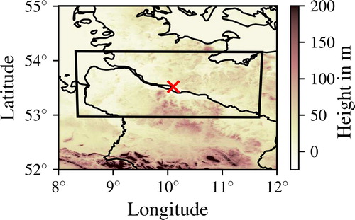
COSMO is a limited-area, non-hydrostatic numerical weather prediction model, developed and maintained by the COnsortium for Small-scale MOdelling. It is a convection-permitting model and is operationally used for weather prediction in mesoscale (Baldauf et al., 2011) with resolutions up to 1 km. We use COSMO here with a higher horizontal resolution of 450 m, in a set-up called COSMO-HH. The model area spans a region around Hamburg with 500 × 300 grid points, which equals roughly 220 × 130 km (Fig. 1). This high horizontal resolution allows us to resolve large eddies (Heinze et al., 2017). We use a 3D-turbulence scheme with prognostic equations for the advection of turbulent kinetic energy, which was developed for the LITFASS project (Herzog et al., 2002), and only subgrid scale eddies are parametrized.

Fig. 1. Surface height in meters for the metropolitan area of Hamburg. The black rectangle is showing used model area, and the red cross is marking the position of the Wettermast Hamburg. Data are based on NASA JPL (2013).

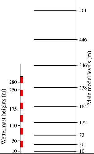
Terrain-following vertical coordinates are used in COSMO. We use a well-tested vertical level set-up with 50 full vertical levels (see also Fig. 2 for levels in the lowest 600 m). Too high vertical resolutions for an untuned set-up can lead to unphysical oscillations (Buzzi, 2008). This configuration of COSMO is tuned towards this vertical level set-up, as it was previously used as operational model at the DWD. Furthermore, comparable studies indicate that the vertical resolution is not as important as the horizontal resolution for the nocturnal boundary layer (Boutle et al., 2016; Kleczek et al., 2014; Steiner et al., 2014). TERRA-ML (Schrodin and Heise, 2001) with seven soil layers is utilized as soil model and provides lower boundary conditions for COSMO-HH.

Fig. 2. Wettermast levels (except 2-m height) and main model levels for COSMO-HH in the lowest 600 m.

Our surface heights (shown in Fig. 1) are derived from a digital elevation model, which is calculated on basis of the Shuttle Radar Topography Mission (Farr et al., 2007; NASA JPL, 2013). To estimate soil types, we further use the soil map of Germany (‘Bodenübersichtskarte’) (Bundesanstalt fuer Geowissenschaften und Rohstoffe, 2016), while the land use classification is based on the CORINE Land Cover inventory (Keil et al., 2011)

2.3. Wettermast Hamburg

The Wettermast Hamburg is a 300-m-tall broadcasting tower located in northern Germany, south-east of Hamburg (${53.5192}^{°}\mathrm{N}$ and ${10.1029}^{°}\mathrm{E},$ denoted as red cross in Fig. 1). The surrounding area around the Wettermast Hamburg can be characterized by shallow industrial buildings in westerly and northerly direction and rural areas in southerly and easterly direction. The main city area of Hamburg is about 7 km away from this tower. We refer to Brümmer et al. (2012) for more information about the tower and the measurements on this site.

We use U-wind, V-wind, temperature and relative humidity measurements from seven different heights (2, 10, 50, 110, 175, 250 and 280 meters, see also Fig. 2 for a schematic overview in comparison with the main model levels). The measurements in 2 m and 10 m are observed at a smaller tower in about 200-m distance to the main tower. This distance is smaller than our grid spacing, and we assume that all measurements are at the same horizontal position. To obtain more stable estimates, we averaged all measurements on a 10 minutes’ basis. The measurement instruments, measurement heights and instrumental accuracy can be seen in Table 3.

Table 3. The used measurements at the Wettermast Hamburg with measurement instrument, heights and instrumental accuracy.

Parameter	Instrument	Height in m	Accuracy
Temperature	PT-100	2, 10, 50, 110, 175, 250, 280	0.1 K
Relative humidity^a	HMP 45	2, 10, 50, 110, 175, 250, 280	2%–3%
U- and V-wind	Sonic USA-1	10, 50, 110, 175, 250, 280	0.1 m s^−1

^a The used instrumental accuracy of HMP 45 for relative humidity is humidity dependent, and we only can specify a range of possible accuracies.

We interpolate model output by nearest neighbour to the horizontal position and linearly to heights of the Wettermast Hamburg. The derived wind speed is the square root of the sum of squares of U-wind and V-wind component. We further define the temperature stratification (hereafter stratification) of the i-th height as normalized and discretized vertical potential temperature gradient $\frac{\partial \theta }{\partial \mathrm{z}}$ between the i + 1-th and i – 1-th height as $${\left(\frac{\partial \theta }{\partial \mathrm{z}}\right)}_i=\frac{{\theta }_{i+1}-{\theta }_{i-1}}{{\mathrm{z}}_{i+1}-{\mathrm{z}}_{i-1}}·100.$$

3. Experiments

In this section, we describe shortly our experimental set-up and the synoptic conditions of our three test cases.

3.1. Experimental set-up

We use an ensemble data assimilation system with 40 ensemble members. The lateral boundary conditions are given by operationally used ICON-EPS runs with the same number of ensemble members (Winkler et al., 2018). These runs have over Europe a horizontal resolution of 20 km. The lateral boundary conditions have thus a horizontal resolution refinement factor of ∼44 times the horizontal resolution of COSMO-HH. A similar refinement factor was used in previous studies (Schraff et al., 2016). We use only test cases with low wind speed. We thus expect that small-scale processes are more important than large-scale processes, and the impact of the lateral boundary conditions can be neglected. The ICON-EPS runs are initialized at 1200 UTC and 0000 UTC based on analyses made by an ensemble data assimilation system. Hourly ICON-EPS forecasts are used in between these analyses.

We perform three different experiments for every test case, where we assimilate different variables from the Wettermast Hamburg (see also Table 4 for assimilated variables). A control run (hereafter CONTROL) without any data assimilation is our baseline experiment. We only assimilate U- and V-wind in the WIND experiment, which is used to see an observation impact from wind components only. In the ALL experiment, we additionally assimilate temperature and relative humidity. This last experiment is used as comparison to estimate an observation impact of wind components relative to assimilation of the full tower data. In all assimilation experiments, we use an hourly assimilation window, where we assimilate available 10-minute averages in all available heights.

Table 4. Experiment names and assimilated variables.

Experiment	Assimilated variables
CONTROL	–
WIND	U- and V-wind
ALL	T, RH, U- and V-wind

We initialize every experiment at 1200 UTC based on interpolated ICON-EPS analyses. All experiments are run up to 0600 UTC the following day. While we generate an 18-hour control forecast, without data assimilation, in the CONTROL experiment, we use an hourly analysis cycle for the WIND and ALL experiment. This analysis cycle is used to generate an analysis and also an hourly first guess forecast (in the following called background forecast). For the experiments with assimilation, we run additional 6-hour control forecast initialized from corresponding analyses at 0000 UTC. We can compare analysis cycle and control forecasts with these 6-hour control forecasts. We can further use them to estimate an accumulated observation impact of the previous 18-hour cycling on longer lead times in the nocturnal boundary layer.

3.2. Test cases

The wind profile is connected to stratification via turbulence in the boundary layer. These two quantities are especially related in the stably stratified nocturnal boundary layer. All three test cases have synoptic conditions where a stably stratified boundary layer developed or prevailed at night time. All test cases further have a strong wind speed decrease in 50-meter height compared to previous day time, indicating that turbulence was decreased at night time.

The first test case (07 June 2016) is representative of a typical stably stratified nocturnal boundary layer in summer. Because of high pressure influence, almost no cloud was formed around the Wettermast Hamburg, while low clouds were advected into the western part of the domain. At the Wettermast Hamburg, there was a weakly stratified nocturnal boundary layer with potential temperature differences of 4 K (284.8 K in 2-metre height and 288.6 K in 280-metre height) at 0300 UTC, and the boundary layer height was in 300 m.

The second test case (26 October 2016) has a strongly stratified nocturnal boundary layer with one fog layer at the ground and a low cloud layer in 175 m. As a result of high pressure and advection of cold air, the 2-metre temperature decreased rapidly in the evening, starting from around 282 K (at 1700 UTC) down to 274.7 K (at 0100 UTC). This led to potential temperature differences up to 7 K (273 K in 2-metre height and 279.8 K in 280-metre height at 0300 UTC) at night time. The nocturnal boundary layer height was relatively low with heights between 50 and 110 m.

The third test case (12 November 2016) is characterized by a strong inversion in lower heights. This inversion was induced by radiative cooling and by cold and dry air advection due to withdrawing of a low pressure system during day time. At night time, the wind direction veered from south-westerly winds to south-easterly winds in 10-m and 50-m height, leading to a temperature decrease in lower heights. As a consequence, the stratification was amplified with differences in the potential temperature of around 6 K (267.8 K in 2-metre height and 274.1 K in 280-metre height at 0300 UTC).

4. Results and discussion

In the following, we will present and discuss our results with regard to the observation impact of wind profile observations in the nocturnal boundary layer. We will firstly concentrate on quantitative observation impact measures, while we will show qualitatively differences between our test cases in the second part.

We want to estimate the observation impact of wind profile observations in the atmospheric boundary layer. To assess an overall observation impact on the ensemble, we can use the analysed increment of the ensemble mean $\delta {\overline{\mathbf{x}}}^{\mathrm{a}}$ in (1). The expected value of this increment is zero, if model and observations are unbiased. We can analyse the increments of the ensemble mean averaged over all test cases to discover similarities between different variables and experiments. If a variable is influenced by data assimilation, its mean absolute increment (MAI) is always larger than zero, showing an observation impact on the ensemble mean of this variable.

To see the overall observation impact of the wind variables in absolute and relative terms, we will analyse the mean increments and MAIs in observation space at the Wettermast Hamburg (Fig. 3a–d). To compare the impact on different variables, we normalized the increments by their observational error standard deviations (Table 2).

Fig. 3. Normalized increment for different variables in (a) & (b) the WIND experiment and (c) & (d) the ALL experiment. (a) & (c) represent the mean absolute increment, while (b) & (d) are the mean increment. Different coloured bars show an observation impact on different variables. Shown increments are normalized by their observation errors. Values are calculated based on ensemble mean of analysis and background for all analysis times and all heights starting in 10 meters at the Wettermast Hamburg. The black lines represent the bootstrapped 5% and 95% percentile based on 1000 samples.

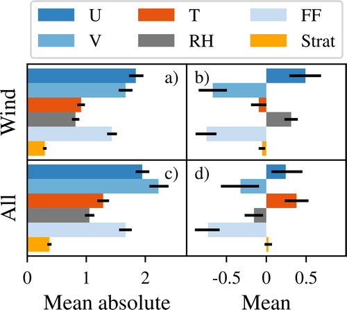
The normalized MAIs for wind components and wind speed are larger than for temperature, relative humidity and stratification in the WIND experiment (Fig. 3a). We assimilate wind components, instead of wind speed and direction; thus, the observation impact on the wind components is up to 1.3 times larger than on the wind speed. There is further some impact on temperature and relative humidity (up to MAI ≈ 0.9), while the impact on stratification (MAI ≈ 0.3) is negligible.

Assimilation of wind components decreases wind speed and the V-wind component in mean, while the U-wind component is increased (Fig. 3b). The changes of wind components are smaller than for wind speed, because of fluctuating increments in time, indicated by wider error bars compared to the MAI. These normalized mean increments for wind variables have the same direction and order of magnitude as the mean errors of the CONTROL experiment compared to observations (Table 5) and are induced by biases in the model or lateral boundary conditions. Because of model biases, it is known that COSMO tends to overestimate the wind speed in stably stratified boundary layers (Cerenzia, 2017). This overestimation explains the distinct direction of correction for the V-wind component and the wind speed in the WIND experiment. The normalized mean increments for temperature, relative humidity, and stratification are much smaller than for wind variables. The normalized mean increments for temperature and relative humidity have also an altering direction as one would expect by the mean errors of the CONTROL experiment. This shows that existing model biases for temperature, stratification and relative humidity are not corrected by assimilation of the wind components.

Table 5. Mean error between ensemble mean in CONTROL experiment and Wettermast Hamburg for U- and V-wind component, temperature, relative humidity, wind speed and stratification. The mean error is estimated over all three test cases and all heights, starting in 10 meters at the Wettermast Hamburg.

Variable	Mean error
U-wind	–0.05 m s^−1
V-wind	0.56 m s^−1
Temperature	–0.09 K
Relative humidity	0.93 %
Wind speed	0.48 m s^−1
Stratification	0.11 K (100 m)^–1

The comparison between MAI and mean increments for the WIND experiment reveals that there is an essential observation impact on almost all variables, which cannot be attributed to bias correction. This observation impact is also evident in non-assimilated variables, such as temperature and relative humidity.

The number of assimilated observations is more than doubled in the ALL experiment (156 observations per hour) compared to the WIND experiment (72 observations), and we would expect that the observation impact scales with the number of observations. Nevertheless, additional assimilation of temperature and relative humidity observations increases the impact on temperature by only up to 40% compared to the WIND experiment (Fig. 3c). This discrepancy shows that there is a redundancy in observation impact between the two experiments. The wind variables have further a similar impact on temperature and relative humidity as additional observations of the latter one, suggesting the importance of wind observations for data assimilation.

By assimilating additional temperature and relative humidity, we also nudge the model towards these observations. Model biases of temperature and relative humidity in the background have thus an impact on the normalized mean increments in the ALL experiment (Fig. 3d). This leads to an increase of the mean increment in temperature compared to the WIND experiment, while the mean increment in relative humidity is decreased. This fact indicates that the covariance-driven relationship between temperature and wind in the ensemble has an alternating direction compared to the relationship in errors. As a consequence, the magnitude of the normalized mean increments in the wind components is also decreased in the ALL experiment compared to the WIND experiment.

Assimilation of wind profile observations has a larger observation impact on increments of wind variables than temperature and relative humidity. The changes due to assimilating additional temperature and relative humidity observations are small beside bias correction as shown in the MAI.

While we have shown the overall observation impact at the Wettermast Hamburg, we will now investigate the observation impact in spatial terms (Fig. 4).

Fig. 4. Mean absolute increment of wind speed (top) and temperature (bottom) for WIND (left) and ALL experiment (right) at the second lowest model level (∼35 m above ground). The spatial average is shown as additional information, while position of the Wettermast Hamburg is marked by a black cross. Land-sea and German state borders are displayed as dark grey contour lines (based on GeoBasis – DE/BKG 2018). (a) Mean = 0.59 m/s, (b) mean = 0.72 m/s, (c) mean = 0.40 K and (d) mean = 0.45 K.

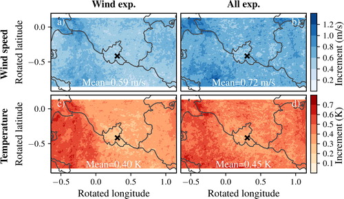
The unnormalized MAI has a similar spatial distribution for wind speed (Fig. 4a,b) and temperature (Fig. 4c,d) for the second lowest model height (∼ 35 m above ground). The impact of the WIND experiment (Fig. 4a,c) is comparable in its spatial distribution to the ALL experiment (Fig. 4b,d). Spatial mean MAIs of the WIND experiment have further a similar order of magnitude (more than 80%) to the means of the ALL experiment. This reveals a similar spatial observation impact of wind components compared to additional assimilation of temperature and relative humidity. We can state that the observation impact of wind profile observations on the increments is large compared to the added value of additional temperature and relative humidity assimilation.

In the western part of the domain, the observation impact is increased compared to other grid points. This represents some synoptical features, induced by low clouds on 07 June 2016, showing that this feature is simulated within our experiments. The observation impact is decreased for the main city of Hamburg compared to rural areas outside the city, despite its closeness to the Wettermast Hamburg. We therefore conclude that observations at the Wettermast Hamburg are more representative for the rural area around Hamburg than for the main city in our model configuration.

In the following, we will analyse an observation impact of wind profile observation on the analysis and forecast error in the WIND experiment. We use here ratios of root-mean-squared errors (RMSE) between analyses and background forecasts, and background forecasts and the CONTROL experiment for different variables (Fig. 5) at the Wettermast Hamburg.

Fig. 5. Quotient of RMSE between ensemble mean in analysis and in background forecast (a) and quotient of RMSE between ensemble mean in background forecast and for CONTROL experiment (b). Ratios are valid for WIND experiment and are averaged over all analysis times and all heights, expect 2-meter height. Coloured bars have the same meaning as in Figure 3. The black lines represent the bootstrapped 5% and 95% percentile based on 1000 samples.

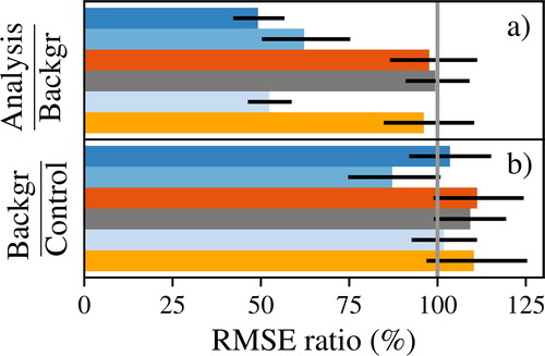
Assimilation of wind components decreases the RMSE of wind, temperature, relative humidity and stratification in the analyses compared to hourly background forecasts (Fig. 5a). In particular, the error in wind components and wind speed is decreased, while the error decrease in temperature, relative humidity and stratification is negligible compared to bootstrapped uncertainties.

We can estimate an indirect observation impact due to propagation by comparison between background forecasts and the CONTROL experiment without data assimilation (Fig. 5b). For the background forecasts, assimilation of wind components has a neutral impact on wind variables, while the error for temperature, relative humidity and stratification is insignificantly increased. The positive impact of assimilating wind components dissipates in time such that almost no impact remains after an hour lead time as indicated by the uncertainties.

In our test cases, the low-level jet above the nocturnal boundary layer is mostly within heights of the Wettermast Hamburg, and small model deviations in boundary layer height can lead to large errors in wind speed. The RMSE of wind speed within the CONTROL experiment increases with height (Fig. 6), which can be explained by systematic underestimation of the low-level jet by COSMO (Buzzi et al., 2011; Steiner et al., 2014).

Fig. 6. The assimilation impact (a), defined as RMSE difference between WIND and CONTROL, for wind speed in 50-m height. Root-mean-squared error of wind speed for (b) analysis (solid lines, left) and for (c) forecasts with one-hour lead time (dashed line, right) against observations as function of height and based on all run times. Three experiments are shown as different colours (Orange: WIND experiment; Grey: ALL experiment). The values for the blue CONTROL experiment are almost the same in (b) and (c), the differences are caused by the time shift of one hour. Displayed error bars and the tube are calculated based on bootstrapping with 1000 samples and represent the 5% and 95% percentile of the RMSE. The error bars for the ALL experiment in (b) and (c) are not shown, because they are almost the same as for the WIND experiment.

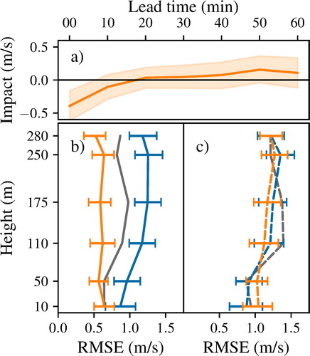
At analysis, the model error is significantly decreased by assimilation of wind components, especially in heights of the low-level jet. The positive observation impact diminishes with lead time (Fig. 6a). After 20 minutes, almost no observation impact is left, while afterwards we have a negative assimilation impact. This is caused by model errors and miss-represented processes as we will show later. Additional assimilation of temperature and relative humidity increases the error compared to the WIND experiment, especially in upper heights (Fig. 6b). This indicates a negative impact of temperature and relative humidity on the analysis of wind speed in heights of the low-level jet.

Forward propagation in time increases the RMSE compared to analysis in the WIND and ALL experiment (Fig. 6c). For assimilation of wind components, some small positive observation impact remains compared to the CONTROL experiment in heights above 50 m. Nevertheless, these RMSE differences between different experiments are insignificant, and we cannot say if they are by chance. This also shows that additional assimilation of temperature and relative humidity profile has only a small impact on the forecast.

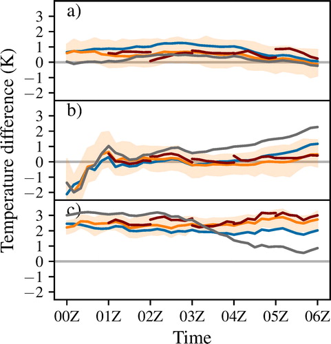
To analyse an observation impact on longer lead times across the three test cases, we will assess the forecast impact qualitatively with six-hour control forecasts started at 0000 UTC for wind speed (Fig. 7) and temperature (Fig. 8).

Fig. 7. Time series of wind speed difference between interpolated model output and observations in 50-meter height for all three test cases (a for 07 June 2016, b for 25 October 2016 and c for 12 November 2016). Four different colours show four different types of forecast (Blue: CONTROL experiment without assimilation; Orange: six-hour forecast started with analysis of WIND experiment at 0000 UTC; Red: analysis cycle of WIND experiment; Grey: six-hour forecast started with analysis of ALL experiment at 0000 UTC). Solid lines display the ensemble mean, while orange tubes are estimated ensemble spread based on 5% and 95% percentile of WIND experiment’s control forecast.

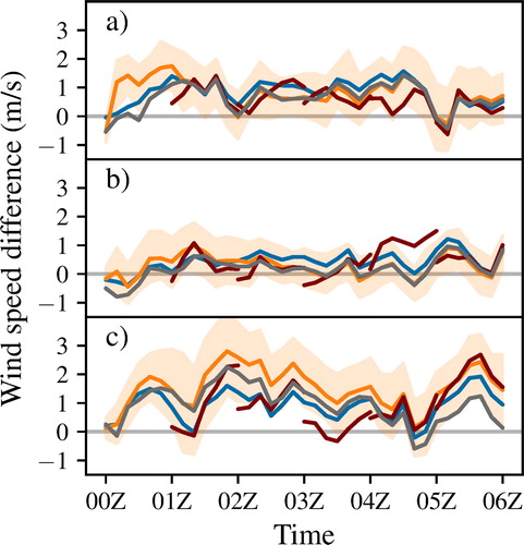
Fig. 8. Time series of temperature differences between interpolated model output and observations in 50 meter height for all three test cases (a for 07 June 2016, b for 25 October 2016 and c for 12 November 2016). Four different colours show four different types of forecast (Blue: CONTROL experiment without assimilation; Orange: six-hour forecast started with analysis of WIND experiment at 0000 UTC; Red: analysis cycle of WIND experiment; Grey: six-hour forecast started with analysis of ALL experiment at 00 UTC). Solid lines display the ensemble mean, while orange tubes are the ensemble spread based on 5% and 95% percentile of WIND experiment’s control forecast.

The wind speed is overestimated across all three test cases and in all experiments in 50-m height (Fig. 7), yet all forecasts have a high similarity in their temporal development. The cumulative effect of wind components assimilation up to 0000 UTC generally decreases the forecast error in two of three test cases (Fig. 7a,b), showing a positive observation impact on forecasts. The ensemble spread of the WIND experiment is also large enough to cover almost all different experiment trajectories. Nevertheless, the spread is sometimes too small to explain differences between forecasts and observations. This indicates that we have a reasonable ensemble spread, while also uncovered biases remain in the forecasts. These biases cannot be reduced by additional assimilation of temperature and relative humidity on 07 June 2016 and 25 October 2016, because the potential to correct possible wind speed deviations is already covered by the wind components. In the first two test cases, the assimilation impact diminishes after 4-hour lead time, which is longer than the previously shown 40 minutes (Fig. 6a).

On 12 November 2016 (Fig. 7c), the errors in wind speed have the highest magnitudes across all test cases. Here, the forecast error of the WIND experiment is increased compared to the CONTROL experiment. This deviation can be partially corrected by additional assimilation of temperature and relative humidity. The forecast error of the ALL experiment is nevertheless increased compared to the CONTROL experiment before 0400 UTC. There have to be some important processes, which cannot be reproduced by our forecasting system.

Additional assimilation of wind components within the shown time windows has a negligible impact on forecast of the wind speed. While overestimation is decreased at analysis, the trajectories backdrop to previous biases with increasing lead time. This backdropping explains the 40-minute memory time in Fig. 6. The overestimation of wind speed within the nocturnal boundary layer cannot be corrected by wind observations. This indicates intrinsic problems of COSMO or a too strong forcing by the lateral boundary conditions in this test case.

The forecast error decrease after 0400 UTC is only identifiable in the ALL experiment. This suggests that problems in this test case might be related to temperature and relative humidity. Despite these problems, we can say that assimilation of wind components has a positive observation impact on the forecast of wind speed, while improvements due to additional assimilation of temperature and relative humidity are only discernible in the last test case.

At the beginning of the shown six hours, the forecast error of the WIND experiment equals almost the forecast error of the CONTROL experiments in two cases (Fig. 8a,b). With lead time, the forecast error is improved in the WIND experiment compared to the CONTROL experiment in these two cases. This shows that the impact of the wind profile assimilation is propagated to the temperature in time via an improved estimate of the turbulence. The memory time of the assimilation impact is four hours for the first test case (Fig. 8a), which is similar to the memory time within the wind speed (Fig. 7). The negative assimilation impact for the ALL experiment in the second test case (Fig. 8b) is induced by fog. Whereas COSMO represents the fog feature, the additional assimilation of temperature and relative humidity leads to a too thick continuous layer of fog. This reduces the effect of radiative cooling on the temperature and induces a positive bias in the temperature for the ALL experiment.

On 12 November 2016 (Fig. 8c), the temperature is overestimated by all models, which cannot be compensated by the ensemble. In this case, assimilation of wind components increases the error compared to the CONTROL experiment for forecast and analysis. The forecast error of the ALL experiment is further increased in the first forecast hours. After 0230 UTC, the temperature forecast of the ALL experiment improves, leading to a decreased error compared to the CONTROL experiment, which is not apparent in the WIND experiment. This improvement in temperature is advanced compared to the results for wind speed. These problems in this test case are thus induced by processes with a direct impact on the temperature forecast.

In Figs. 7 and 8, we compared different experiment for a single height. To further understand what processes are leading to given overestimation of wind speed and temperature, we analyse the vertical profile of wind speed and potential temperature at 0300 UTC for all three test cases (Fig. 9).

Fig. 9. Modelled and observed wind speed (FF, a, b & c) and potential temperature (TP, d, e and f) at 0300 UTC for 07 June 2016 (a & d), for 25 October 2016 (b & e), and for 12 November 2016 (c & f). Transparent orange lines are 40 ensemble members from forecast of WIND experiment based on analysis at 0000 UTC, while the ensemble mean from this forecast is shown as bold orange lines with crosses as marker. The blue line is the ensemble mean CONTROL experiment, while the forecast of the ALL experiment is displayed in grey. The red line is the analysis of the WIND experiment at 0300 UTC, nudged towards the black observations.

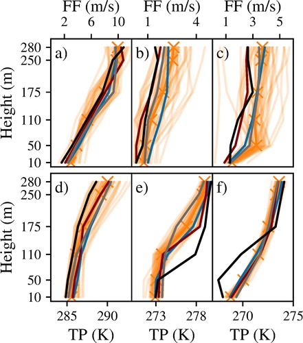
The wind speed is overestimated compared to observations in all heights (Fig. 9a–c). Despite this bias, the observations are covered by at least some ensemble members. We can state that the ensemble spread in the WIND experiment is large enough to cover these differences. Similar to previous results, the differences between observed and forecasted wind profile are decreased for the WIND experiment compared to the CONTROL experiment in two of three test cases (Fig. 9a,b). Additional assimilation of temperature and relative humidity decreases the forecast error compared to the WIND experiment in cases where latter one has a negative impact (Fig. 9c). The negative impact seems to be connected to biases in temperature and/or relative humidity.

On 12 November 2016 (Fig. 9c), most forecast ensemble members have problems to represent the observed low-level jet, and they have their highest wind speeds above 175 m. Furthermore, the observed low-level jet in 175 m is only partially modelled by some ensemble members, whereas the low-level jet is missed for all ensemble means. The wind speed in 50-meter height is also overestimated by almost all ensemble members compared to observations. Here, the assimilation experiments have a negative impact on the forecast of the wind speed in the boundary layer, which can be also seen in Figs. 7 and 8. This can be explained by assimilation of the wind components, which nudges the wind speed to observations. This nudging seems to disturb the model in its equilibrium on this test case, leading to an assimilation shock.

The model bias compared to observations is caused by missing cold air advection in 50 and 110 meters (Fig. 9f). This missing cold air advection also explains the difficulties to represent this test case with COSMO. In reality, this cold air advection was caused by a wind shift to easterly directions. This phenomenon often occurs at the Wettermast Hamburg in stably stratified nocturnal boundary layers and can be partially explained by local circumstances and the urban heat island of Hamburg. Nevertheless, COSMO cannot simulate these local processes, because its resolution seems to be too coarse and the city effects are also only roughly parameterized by TERRA-ML. We can thus expect that we can improve the representation of these local circumstances by properly modelling the city effects. Large-eddy simulations with few meters horizontal resolution might be necessary to fully resolve the dominating processes in this test case (van Stratum and Stevens, 2015).

We can observe the same data assimilation effects on potential temperature as for the wind speed (Fig. 9d–f). Assimilation of wind profile data has a positive impact on the forecast of the temperature in cases, where the model can represent the underlying processes. If errors due to missing processes are not represented by the ensemble, the corresponding state estimates cannot be improved by an EnKF. This leads to forecast degradation in all variables in cases with large model errors. This is especially the case if no ensemble member can correctly represent the boundary layer height (Fig. 9e,f). Then, the boundary layer height cannot be corrected. Not only the boundary layer height is systematically overestimated, but also the temperature gradients are smoothed out. This tendency can be explained by the overestimation of the wind speed in COSMO, leading to an overestimation of the turbulence. As a consequence, we can say that we need to reduce the overestimation of the wind speed to improve the forecast of nocturnal boundary layer.

As seen in two of three test cases, the nocturnal boundary layer is difficult to model with its temporal and spatial small-scale phenomenon. Despite this, we can conclude that assimilation of wind components improves the forecast of wind speed in the nocturnal boundary layer. Additional assimilation of temperature and relative humidity has here only a limited added value. Further, we can improve the forecast of temperature by assimilation of wind profile observations, especially in weakly stratified nocturnal boundary layers.

5. Summary and conclusion

There is an increasing potential of wind profile observations for data assimilation in the boundary layer, but the observation impact is unknown. In this study, we analysed this assimilation impact of wind profile observations on the forecast of a high-resolution COSMO set-up around the metropolitan area of Hamburg. A LETKF implemented in KENDA-COSMO was used as data assimilation framework to assimilate observations hourly for three different test cases with stably stratified nocturnal boundary layers. Two of these three test cases have a strongly stratified nocturnal boundary layer, which is difficult to represent with COSMO.

We show that wind profile observations have an observation impact in terms of MAIs in spatial and temporal dimensions. We further find a positive or neutral observation impact of wind profile observations on all variables at analysis. Further, we improve the wind speed forecast in two of three cases, while additional assimilation of temperature and relative humidity had almost no impact. The positive observation impact of wind profile observations on the wind is propagated over time to the temperature, while the impact on the analysis of the temperature is negligible. These results correspond to the expectation that turbulence is the driving factor of the nocturnal boundary layer. We can use wind observations to correct errors in the turbulence, and hence, in the nocturnal boundary layer. The connection between wind and nocturnal boundary layer is thus revealed by the propagation step of the ensemble Kalman filter. We further show that the memory time for the wind speed and our single tower observations is 4 hours, if the dominating processes are represented within COSMO.

The third test case is the most difficult test case, because advection of cold air is missed by almost all forecast ensemble members. This missed advection causes a bias in the wind forecast. The assimilation of wind components does not improve the forecast in this test case. Here, assimilation nudges the forecast to the observations and disturbs the model in its equilibrium. Additional assimilation of temperature and relative humidity improves the forecast later in the night. Thus, we can probably avoid the negative impact by additional assimilation of other observations at other locations, which can also increase the memory time of the assimilation. We do not prove this point in this study, because there is only one single tall tower equipped with measurement devices in our studied region. To combine wind observations from different sources, geo-statistical methods might be needed. These additional geo-statistical methods can help to decrease the discrepancy in representing the wind between model forecast and observations (Bédard et al., 2015).

COSMO has problems to correctly represent strongly stratified nocturnal boundary layers. These problems are especially evident with the low-level jet in the third test case, while there are also some problems related to fog and radiative cooling, leading to biases within the temperature. Nevertheless, we prove that we can create an analysis of the nocturnal boundary layer with tall tower profile observations and a sub-kilometre-scale data assimilation framework, if the forecast model can represent governing influences on the nocturnal boundary layer. All in all, the limiting factor for the improvement by assimilation is the ensemble spread and the used forecast model. We therefore expect that we can further improve the results with an improved forecast model. Higher horizontal resolutions together with large-eddy simulations might be needed to fully represent the dominating processes in the nocturnal boundary layer (van Stratum and Stevens, 2015). Based on our results, we conclude that horizontal resolution, the land model and properly representation of turbulent processes in the nocturnal boundary layer are more important for modelling the nocturnal boundary layer than the size of the domain or vertical resolution.

Consequently, we infer from our results a high potential of ground-based wind profile observations, like LiDARs, in the atmospheric boundary layer for data assimilation. We expect that this high potential is even more evident, when wind profile observations at diverse positions are assimilated into high-resolution NWP models. Data assimilation of surface-near wind profile observations has therefore the potential to be a missing key for forecast improvements of wind and stratification in the atmospheric boundary layer.

Acknowledgements

We want to acknowledge the Deutscher Wetterdienst, especially Hendrik Reich and Christoph Schraff, for delivering ICON-EPS boundary data and technical help with COSMO-KENDA during the development. Further, we want to acknowledge Ingo Lange for the Wettermast Hamburg data. We want also to acknowledge members of the DFG research unit 2131 ‘Data Assimilation for Improved Characterization of Fluxes across Compartmental Interfaces’ for the help of conducting this study.

Disclosure statement

We have no conflicts of interest to disclose.

Additional information

Funding

This work was supported by the ‘Deutsche Forschungsgemeinschaft’ (DFG, German Research Foundation) under Grant 243358811.

References

- Ancell, B. C., Kashawlic, E. and Schroeder, J. L. 2015. Evaluation of wind forecasts and observation impacts from variational and ensemble data assimilation for wind energy applications. Mon. Weather Rev. 143, 3230–3245. doi:10.1175/MWR-D-15-0001.1
- Anderson, J. L. and Anderson, S. L. 1999. A Monte Carlo implementation of the nonlinear filtering problem to produce ensemble assimilations and forecasts. Mon. Weather Rev. 127, 2741–2758. doi:10.1175/1520-0493(1999)127<2741:AMCIOT>2.0.CO;2
- Baas, P. and Bosveld, F. 2010. Assimilation of Cabauw boundary layer observations in an atmospheric single-column model using an ensemble-Kalman filter. Technical report, Royal Netherlands Meteorological Institute, Netherlands.
- Baldauf, M., Seifert, A., Förstner, J., Majewski, D., Raschendorfer, M. and co-authors. 2011. Operational convective-scale numerical weather prediction with the COSMO model: description and Sensitivities. Mon. Weather Rev. 139, 3887–3905. doi:10.1175/MWR-D-10-05013.1
- Bédard, J., Laroche, S. and Gauthier, P. 2015. A geo-statistical observation operator for the assimilation of near-surface wind data. QJR Meteorol. Soc. 141, 2857–2868. doi:10.1002/qj.2569
- Benjamin, S. G., Schwartz, B. E., Koch, S. E. and Szoke, E. J. 2004. The value of wind profiler data in US weather forecasting. Bull. Amer. Meteor. Soc. 85, 1871–1886. doi:10.1175/BAMS-85-12-1871
- Boutle, I., Finnenkoetter, A., Lock, A. and Wells, H. 2016. The London Model: forecasting fog at 333 m resolution. QJR Meteorol. Soc. 142, 360–371. doi:10.1002/qj.2656
- Brümmer, B., Lange, I. and Konow, H. 2012. Atmospheric boundary layer measurements at the 280 m high Hamburg weather mast 1995-2011: mean annual and diurnal cycles. Metz. 21, 319–335. doi:10.1127/0941-2948/2012/0338
- Bundesanstalt fuer Geowissenschaften und Rohstoffe. 2016. Bodenuebersichtskarte.
- Buzzi, M. 2008. Challenges in operational numerical weather prediction at high resolution in complex terrain. Doctoral thesis. ETH Zurich.
- Buzzi, M., Rotach, M. W., Holtslag, M. and Holtslag, A. A. 2011. Evaluation of the COSMO-SC turbulence scheme in a shear-driven stable boundary layer. Metz. 20, 335–350. doi:10.1127/0941-2948/2011/0050
- Cerenzia, I. 2017. Challenges and critical aspects in stable boundary layer representation in numerical weather prediction modeling: diagnostic analyses and proposals for improvement. PhD thesis. Alma Mater Studiorum Università di Bologna.
- Declair, S., Stephan, K. and Potthast, R. 2015. On the improvement of numerical weather prediction by assimilation of hub height wind information in convection-resulted models. In: EGU General Assembly Conference Abstracts, Vol. 17, Vienna, Austria, 9451.
- Desroziers, G., Berre, L., Chapnik, B. and Poli, P. 2005. Diagnosis of observation, background and analysis-error statistics in observation space. QJR Meteorol. Soc. 131, 3385–3396. doi:10.1256/qj.05.108
- Farr, T. G., Rosen, P. A., Caro, E., Crippen, R., Duren, R. and co-authors. 2007. The shuttle radar topography mission. Rev. Geophys. 45, RG2004, doi:10.1029/2005RG000183
- Gaspari, G. and Cohn, S. E. 1999. Construction of correlation functions in two and three dimensions. QJR Meteorol Soc. 125, 723–757. doi:10.1002/qj.49712555417
- Harlim, J. and Hunt, B. R. 2007. Four-dimensional local ensemble transform Kalman filter: numerical experiments with a global circulation model. Tellus A 59, 731–748. doi:10.1111/j.1600-0870.2007.00255.x
- Hasager, C. B., Stein, D., Courtney, M., Peña, A., Mikkelsen, T. and co-authors. 2013. Hub height ocean winds over the north sea observed by the NORSEWInD Lidar Array: measuring techniques, quality control and data management. Remote Sens. 5, 4280–4303. doi:10.3390/rs5094280
- Heinze, R., Dipankar, A., Henken, C. C., Moseley, C., Sourdeval, O. and co-authors. 2017. Large-eddy simulations over Germany using ICON: a comprehensive evaluation. QJR Meteorol. Soc. 143, 69–100. doi:10.1002/qj.2947
- Herzog, H.-J., Vogel, G. and Schubert, U. 2002. LLM – a nonhydrostatic model applied to high-resolving simulations of turbulent fluxes over heterogeneous terrain. Theor. Appl. Climatol. 73, 67–86. doi:10.1007/s00704-002-0694-4
- Houtekamer, P. L., Mitchell, H. L., Pellerin, G., Buehner, M., Charron, M. and co-authors. 2005. Atmospheric data assimilation with an ensemble Kalman filter: results with real observations. Mon. Weather Rev. 133, 604–620. doi:10.1175/MWR-2864.1
- Houtekamer, P. L. and Zhang, F. 2016. Review of the ensemble Kalman filter for atmospheric data assimilation. Mon. Weather Rev. 144, 4489–4532. doi:10.1175/MWR-D-15-0440.1
- Hu, H., Sun, J. and Zhang, Q. 2017. Assessing the impact of surface and wind profiler data on fog forecasting using WRF 3DVAR: an OSSE study on a dense fog event over North China. J. Appl. Meteorol. Climatol. 56, 1059–1081. doi:10.1175/JAMC-D-16-0246.1
- Hunt, B., Kalnay, E., Kostelich, E., Ott, E., Patil, D. and co-authors. 2004. Four-dimensional ensemble Kalman filtering. Tellus A 56, 273–277. doi:10.3402/tellusa.v56i4.14424
- Hunt, B. R., Kostelich, E. J. and Szunyogh, I. 2007. Efficient data assimilation for spatiotemporal chaos: a local ensemble transform Kalman filter. Physica D 230, 112–126. doi:10.1016/j.physd.2006.11.008
- Ingleby, B. 2015. Global assimilation of air temperature, humidity, wind and pressure from surface stations. QJR Meteorol. Soc. 141, 504–517. doi:10.1002/qj.2372
- Keil, M., Bock, M. and Esch, T. ( 2011. ). CORINE Land Cover 2006 - Europaweit harmonisierte Aktualisierung der Landbedeckungsdaten für Deutschland. Technical report, Umweltbundesamt.
- Kleczek, M. A., Steeneveld, G.-J. and Holtslag, A. A. M. 2014. Evaluation of the weather research and forecasting mesoscale model for GABLS3: impact of boundary-layer schemes. Boundary-Layer Meteorol. 152, 213–243. doi:10.1007/s10546-014-9925-3
- Miyoshi, T. 2005. Ensemble Kalman filter experiments with a primitive-equation global model. PhD thesis, University of Maryland.
- Mylonas, M., Barbouchi, S., Herrmann, H. and Nastos, P. 2018. Sensitivity analysis of observational nudging methodology to reduce error in wind resource assessment (WRA) in the North Sea. Renewable Energy 120, 446–456. doi:10.1016/j.renene.2017.12.088
- NASA JPL. 2013. NASA Shuttle Radar Topography Mission Global 3 arc second [Data set].
- Park, S.-Y., Lee, H.-W., Lee, S.-H. and Kim, D.-H. 2010. Impact of wind profiler data assimilation on wind field assessment over coastal areas. Asian J. Atmos. Environ. 4, 198–210. doi:10.5572/ajae.2010.4.3.198
- Rostkier-Edelstein, D. and Hacker, J. P. 2013. Impact of flow dependence, column covariance, and forecast model type on surface-observation assimilation for probabilistic PBL profile nowcasts. Wea. Forecasting 28, 29–54. doi:10.1175/WAF-D-12-00043.1
- Schraff, C., Reich, H., Rhodin, A., Schomburg, A., Stephan, K. and co-authors. 2016. Kilometre-scale ensemble data assimilation for the COSMO model (KENDA). QJR Meteorol. Soc. 142, 1453–1472. doi:10.1002/qj.2748
- Schrodin, R. and Heise, E. 2001. The Multi-Layer Version of the DWD Soil Model TERRA-LM. Technical Report 2, Deutscher Wetterdienst.
- St-James, J. S. and Laroche, S. 2005. Assimilation of wind profiler data in the Canadian Meteorological Centre Analysis Systems. J. Atmos. Oceanic Technol. 22, 1181–1194. doi:10.1175/JTECH1765.1
- Steiner, A., Köhler, C., V. and Schumann, J. 2014. EWeLiNE and ORKA: improving model physics for renewable energy. COSMO User Seminar 2014, Offenbach, 15.
- Stull, R. B., eds. 1988. An Introduction to Boundary Layer Meteorology. Atmospheric and Oceanographic Sciences Library. Springer, Dordrecht.
- van Stratum, B. J. H. and Stevens, B. 2015. The influence of misrepresenting the nocturnal boundary layer on idealized daytime convection in large-eddy simulation. J. Adv. Model. Earth Syst. 7, 423–436. doi:10.1002/2014MS000370
- Wagner, R., Jørgensen, H. E., Paulsen, U. S., Larsen, T. J., Antoniou, I. and co-authors. 2008. Remote sensing used for power curves. IOP Conf. Ser: Earth Environ. Sci. 1, 012059. doi:10.1088/1755-1315/1/1/012059
- Winkler, J., Denhard, M., Frank, H., Rhodin, A., Anlauf, H. and co-authors. 2018. ICON-EPS: the operational global ensemble forecasting system of DWD. In: EGU General Assembly Conference Abstracts, Vol. 20, Vienna, Austria, 13813.
- Yang, S.-C., Kalnay, E., Hunt, B. and Bowler, N. E. 2009. Weight interpolation for efficient data assimilation with the Local Ensemble Transform Kalman Filter. QJR Meteorol. Soc. 135, 251–262. doi:10.1002/qj.353