Perturbation structure and evolution in tropical cyclones Noul and Nepartak based on singular vectors

Abstract

This study examined tropical cyclones (TCs) Noul and Nepartak to demonstrate the evolutions of singular vector perturbations. Perturbations comprise eigen-solutions for dry total energy from two domains with different focuses, namely the TC itself and the background atmospheric flow in East Asia. These perturbations are usually used to construct ensemble members for the probabilistic forecasts of the TC trajectory. The horizontal shapes of the TC singular vectors were consistent with asymmetric flows with the wave number of 1 or 2, with the exception of the azimuthal circulation. Most of their vertical structures had higher amplitudes in upper layers mainly concentrated at approximately 200 − 300 hPa. Thus, the upper part of the perturbations developed first, followed by the lower part over time. This process was the opposite of that noted in background singular vector perturbations in mid-latitude East Asia. Calculations of the transient eddy total energy based on analysis data for the two storms revealed that growth occurred earlier in the upper layer than in the lower layer. The cross-sectional eddy evolution in TCs exhibited a similar process to that of singular vectors. In addition, the cross-section of the three-dimensional E-vector convergence and the zonal profiles of the E-vector component also supported the downward process in TC areas. Mid-latitude E-vector analysis indicated that upward energy propagation was consistent with previous findings.

Keywords:

• dry total energy, E-vector, singular vector

1. Introduction

The development and movement of a tropical cyclone (TC) are related to its structure and the background environmental flow (Chan and Gray, 1982; Chan 1985; Holland, 1983). In theoretical studies (Fiorino and Elsberry, 1989; Li and Wang, 1994; Wang, 2002a, 2002b), TCs are assumed to have axially symmetric flow with an asymmetric beta gyre in the ambient uniform background flow, resulting in a constant easterly flow. These assumptions hypothesise TC’s horizontal spatial structures with idealised basic background flows, thus highlighting dynamic processes without excessive detail. In reality, TCs are not limited to a symmetric part with an asymmetric gyre. For various purposes, the background environmental flow can be defined as a latitudinally variation flow or a shear flow similar to real large-scale subtropical high circulation (Shi et al., 2016). Conversely, other studies (Li, 2006; Tam and Li, 2006) have evaluated TC formation based on analysis data by considering a steady-state basic flow in the background and a transient eddy that varies with time. Thus, this method separates the variables into two parts, namely the perturbation (eddy) and basic (background) states, both of which can vary over time. For example, the basic state can be defined as the time evolution based on a controlled numerical integration, and the perturbation can be regarded as a small deviation from the controlled basic state. The purpose of this approach is to explore interactions of the transient eddy, or perturbations, with the basic flow. This method has been widely adopted in instability studies, ensemble forecasts, and data assimilation (Molteni and Palmer, 1993; Fletcher, 2017; Palmer et al., 2019). In the current study, we followed this approach and adopted control run forecast trajectories from the numerical weather prediction (NWP) model as the basic state. Control run forecasts are based on the initial state without perturbations. Perturbations varying with time resulted in deviations between the ensemble run and the control run (Buizza et al., 1993; Molteni and Palmer, 1993; Buizza and Palmer, 1995; Molteni et al., 1996; Palmer, 1996).

Studies of transient eddies and the mean basic flow over time have demonstrated that they interact closely and that energy can be converted between these two flows (Simmons and Hoskins, 1980; James, 1994). The baroclinic wave, which is approximately equivalent to the transient eddy, can rapidly evolve into a barotropically unstable structure through a nonlinear dynamic process. The rapid development of transient eddies is similar to the optimal perturbation growth rate determined in theoretical studies (Farrell, 1989; Borges and Hartmann, 1992). The optimal perturbations can be determined based on the eigenvectors of the linear and adjoint operators from the barotropic vorticity equation. Subsequently, the calculation of optimal growth perturbations can be replaced by singular vectors in more complex NWP models (Buizza et al., 1993). Singular vectors can be used to obtain optimal growth modes at a finite time for the specific basic flow. This method can enable the theoretical determination of the most diverse and meaningful statistical spread of finite ensemble members. The optimal growth can be estimated based on the kinetic energy, entropy, total energy, and dry total energy of the perturbations (ECMWF, 2018).

Buizza (1994) noted that singular vectors from a local domain would increase the ensemble spread around this domain and result in an unstable development. Buizza (1994) proposed the local projection operator of a singular vector to focus on the atmospheric flow in the target domain. Subsequently, studies of TCs (Barkmeijer et al., 2001; Puri et al., 2001; Peng and Reynolds, 2006; Chen et al., 2009; Wu et al., 2009; Lang et al., 2012) have adopted this local projection operator to analyse TC’s circulation evolution. The local operator projection of singular vectors was used to determine perturbation growth in the vicinity of TC’s circulation, which other methods do not focus on.

The aim of this study was to explore singular vector ensemble perturbation structures in the TC domain and the East Asia mid-latitude domain. Moreover, we assessed transient eddies in analysis data obtained from the TC and East Asia domains. The dry total energy, representing all the perturbation or transient eddy dynamical variables, was used and traced without diagnosing individual variables. The energy evolution pointed to the origin of perturbations, and the energy structures showed unstable characteristics. This study assessed similarities and differences between singular vector perturbations and transient eddies. We calculated singular vectors in two domains because TC movement is determined not only by its structure but also by larger scale background flows, such as the south rim of a subtropical high or the leading flow around the East Asia main trough. Yamaguchi and Komori (2009) and Yonehara (2010) have included a set of singular vector perturbations from a large fixed East Asia target domain to assess changes in basic flow that could affect TC movement. They have combined TC domain singular vectors and East Asia domain singular vectors as a set of ensemble members for TC ensemble prediction. This is also used by the ECMWF (2018) and the TC ensemble prediction system of the Taiwan Central Weather Bureau (CWB). The ensemble perturbations from the singular vectors of these two domains can be used to determine the instability processes in TC circulations and their background large-scale circulations. Using perturbations from these two domains can also efficiently increase the statistical spread of TC’s ensemble tracks.

The low resolution and dry versions of tangent and adjoint models are used in this study for calculating singular vectors for two reasons. First, the dry version reduced the cost of development and operation. Second, the model’s initial uncertainty was first set based on dynamic variables (without humidity). Once these initial perturbations were decided, they were added to the high-resolution NWP model to produce forecasts with humidity and full diabatic processes. Moreover, transient eddies were checked based on analysis data from the two TC cases. We then compared singular vectors and transient eddies in the TC domain and the East Asia mid-latitude domain.

The tropical dynamic process differs from the mid-latitude dynamic process. The evolution of mid-latitude East Asia singular vectors is essentially equivalent to the baroclinic wave development process (Buizza et al., 1993; Molteni and Palmer, 1993). For the TC area, some studies have suggested that the cumulus-scale diabatic effect should be considered for calculating singular vectors (Barkmeijer et al., 2001; Lang et al., 2012). These studies have considered the diabatic process in both the tangent linear and the adjoint models for calculating singular vectors, with the diabatic singular vector reflecting the fine TC structure. However, Lang et al. (2012) also concluded that the diabatic effect was small in a low-resolution model. Therefore, the energy of singular vector perturbations in the TC domain may be due to the internal dynamical instability rather than entirely due to the diabatic process. Synoptic-scale wave train, Rossby wave dispersion, low level easterly waves, and especially the upper layer signals induced by mid-latitude dynamical processes are critical for considerations of TC formation and the dynamic instability of TC movements (Li and Hsu, 2018). This is another reason why we adopted low-resolution tangent linear and adjoint models to calculate singular vectors for dry variables in the current stage.

The remainder of this paper is organised as follows. In Section 2, we explain the definition of dry total energy for singular vector calculation, and singular vector perturbations composited from the two domains are introduced. In Section 3, we show the singular vector perturbation evolutions for two typhoon cases. The transient eddies in the analysis data of these two typhoons are described in Section 4. In the final section, we summarise major findings regarding singular vectors.

2. Perturbations composed of singular vectors

The singular vector derivation is briefly shown in the Appendix. In this study, we define the inner product $〈\dots \mathrm{ },\mathrm{ }\dots 〉$ or the ${\mathbf{L}}_2$-Norm$\Vert \Vert$ of the variable${\mathbf{x}}^{\mathbf{\prime }}$ at the final time$t_f$ as follows: (1) $${\Vert {\mathbf{x}}^{\mathbf{\prime }}(t_f)\Vert }^2=〈{\mathbf{x}}^{\mathbf{\prime }}(t_f),\mathbf{E}{\mathbf{x}}^{\mathbf{\prime }}(t_f)〉,$$(1) where E is the weighting operator and the inner product is the global domain integration (ECMWF, 2018). That is (2) $$〈{\mathbf{x}}^{\mathbf{\prime }}(t_f),\mathbf{E}{\mathbf{x}}^{\mathbf{\prime }}(t_f)〉={\int }_D^{}{\int }_0^1\frac{1}{2}({u^{\prime }}^2+{v^{\prime }}^2)+\frac{1}{2}\frac{C_p}{\overline{T}}{T^{\prime }}^2\mathit{\text{dσdD}}+{\int }_D^{}\frac{1}{2}{R}_a\overline{T}\frac{{p^{\prime }}_s^2}{{\overline{p}}_s^2}dD.$$(2)

This equation represents the dry total energy for the present study. The column vector ${\mathbf{x}}^{\mathbf{\prime }}$ is defined as ${(u^{\prime },v^{\prime },T^{\prime },{p^{\prime }}_s)}^{\mathbf{T}}.$ D refers to the global domain or any other chosen domain, and $\sigma$ represents the sigma layer of the model. The weighting operator can be obtained as follows: (3) $$\mathbf{E}=\frac{1}{2}\mathbf{d}\mathbf{iag}(1,\dots ,1,\dots ,\frac{C_p}{\overline{T}},\dots ,\frac{R_a\overline{T}}{{\overline{p}}_s^2},\dots ),$$(3) where $\overline{T}=270\mathrm{ }\mathrm{K}$ and ${\overline{p}}_s=1000$ hPa, which denote the reference temperature and reference pressure, respectively. The other constants are C_p = 1004.24 J/K kg and R_a = 287 J/K kg.

We can define various areas by using the operator D (as shown in the Appendix) to focus on specific atmospheric circulation patterns. For example, in this study, we consider the moving area of 15 longitudinal degrees by 10 latitudinal degrees around the typhoon centre. Singular vectors calculated using Equation (A14)(A14) $$\tilde{\mathbf{G}}={\mathbf{E}}^{1/2}\mathbf{G}{\mathbf{E}}^{-1/2}={\mathbf{E}}^{-1/2}{\mathbf{L}}^{\mathbf{T}}\mathbf{D}\mathbf{EDL}{\mathbf{E}}^{-1/2}.$$(A14) represent the most unstable perturbations in the typhoon circulation. However, large-scale circulations also affect typhoon movement. We define the East Asia domain as ${20}^{\circ }-{60}^{\circ }\mathrm{N}$ and ${100}^{\circ }-{180}^{\circ }\mathrm{E}$ to obtain singular vectors for background perturbations, which yield different possible TC movements (Yamaguchi and Komori, 2009; Yonehara, 2010).

Considering the computational cost, we based the singular vector calculation on the T42L60 CWBGFS resolution. The CWBGFS is the abbreviation of the operational global forecast system in Taiwan Central Weather Bureau. The physics of the adjoint model includes only bi-harmonic diffusion, a simple boundary effect, large-scale precipitation, and a simple Kuo cumulus scheme. A smaller calculation domain results in smaller singular values. In a smaller domain, such as a TC of size ${15}^{\circ }\times {10}^{\circ },$ the largest eigenvalue (EV) $\lambda$ is approximately 8.0; by contrast, in a larger domain, such as the northern hemisphere domain, the largest $\lambda$ can be approximately 60–80 or even larger. We directly use the northern hemisphere singular vector for the perturbation in the ensemble system without increasing its amplitude. When combining singular vectors for the TC and East Asia domains, Yamaguchi and Komori (2009) and Yonehara (2010) have mentioned that they excluded pairs of singular vectors with inner products greater than 0.5. However, we consider that the relative amplitudes of these singular vectors should be determined by different factors. After comparing EVs in the domains, we define two amplitude factors, namely the TC_Factor in the TC domain and the EA_Factor in the East Asia domain. Moreover, to obtain a reasonable perturbation amplitude, we readjust the magnitudes of singular vectors by using the simple NMC method (Parrish and Derber, 1992). Combining these approaches, the ensemble perturbations ${\mathbf{x}}^{\mathbf{\prime }}$ based on the singular vector $v$ are given as follows: (4) $$\begin{array}{c}{{\mathbf{x}}^{\mathbf{\prime }}}_{\text{TC}}=v_{\text{TC}}/\left|v_{\text{TC}}\right|\times \left|\text{NMC}\right|\times \text{TC}\_\text{Factor},\\ {{\mathbf{x}}^{\mathbf{\prime }}}_{\text{EA}}=v_{\text{EA}}/\left|v_{\text{EA}}\right|\times \left|\text{NMC}\right|\times \text{EA}\_\text{Factor},\\ {\mathbf{x}}^{\mathbf{\prime }}={{\mathbf{x}}^{\mathbf{\prime }}}_{\text{TC}}+{{\mathbf{x}}^{\mathbf{\prime }}}_{\text{EA}},\end{array}$$(4) where the TC_Factor is equal to 10 and the EA_Factor is equal to 5. We then estimate the |NMC| factor based on the forecasted variable vector length of the current 24-hour forecast minus the previous day’s 48-hour forecast. The CWBGFS ensemble system setup is shown in Table 1.

Table 1. Arrangement and parameters of the CWB ensemble system for typhoon.

Model	Domain		Resolution	Forecast length
Deterministic	Global Global Global		T511L60	7-day
20 members ensemble			T511L60	7-day
based on
tangent/adjoint			T42L60	48-hour
singular vector	Around TC East Asia	$15°\times 10°$ $100°\mathrm{E}-180°\mathrm{E}$ $20°\mathrm{N}-60°\mathrm{N}$		48-hour

The ensemble prediction system uses the same resolution as the deterministic model in T511L60. They are global spectral models. The tangent/adjoint model in T42L60 is the simplified version of T511L60. The singular vectors are from the dry total energy with two local projection domains. The TC domain is around the TC centre and moves with the TC. The East Asia domain is shown in the table. The optimal finite time of the singular vector is 48-hour.

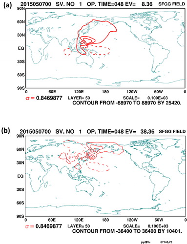
The original horizontal structures of singular vectors calculated using the T42L60 model are depicted in Fig. 1. The first leading singular vectors are chosen from the TC domain (Fig. 1a) and the East Asia domain (Fig. 1b). Notice that the EV of the TC domain is 8.36, which is relatively small compared with that of the East Asia of 38.36. Moreover, the amplitudes of the two singular vectors are different. The singular vector amplitude of the TC domain is approximately double that of the East Asia domain. Although the singular vector amplitude of the TC domain is greater than that of the East Asia domain, the singular vector of the TC domain does not exhibit the same temporal increase as that of the East Asia domain. The EV indicates future growth. To predict the typhoon ensemble track, as expressed in Equation (4)(4) $$\begin{array}{c}{{\mathbf{x}}^{\mathbf{\prime }}}_{\text{TC}}=v_{\text{TC}}/\left|v_{\text{TC}}\right|\times \left|\text{NMC}\right|\times \text{TC}\_\text{Factor},\\ {{\mathbf{x}}^{\mathbf{\prime }}}_{\text{EA}}=v_{\text{EA}}/\left|v_{\text{EA}}\right|\times \left|\text{NMC}\right|\times \text{EA}\_\text{Factor},\\ {\mathbf{x}}^{\mathbf{\prime }}={{\mathbf{x}}^{\mathbf{\prime }}}_{\text{TC}}+{{\mathbf{x}}^{\mathbf{\prime }}}_{\text{EA}},\end{array}$$(4) , we must increase the amplitude of the TC singular vector.

Fig. 1. Original singular vectors from T42L60 model are shown as stream function (m²/s) based on 0000 UTC 7 May 2015 basic flow. (a) The first one singular vector in the TC domain. (b) The first one singular vector in East Asia domain.

3. Singular vector perturbation structures and evolution

3.1. Singular vector horizontal and vertical structures

In this study, two cases, namely Typhoon Noul (lifetime, 1800 UTC 3 May 2015 − 0000 UTC 12 May 2015) and Nepartak (lifetime, 0000 UTC 3 July 2016 − 0000 UTC 9 July 2016), are considered to demonstrate their singular vector perturbation structures and evolutions. The two tracks of these TCs (black lines), their corresponding mean ensemble forecasts (green lines), and control deterministic forecasts (blue lines) are shown in Fig. 2. For convenience, perturbations are defined by differences between ensemble members and the control deterministic forecast in the following discussions. The initial perturbations comprise two-domain singular vectors as shown in Equation (4)(4) $$\begin{array}{c}{{\mathbf{x}}^{\mathbf{\prime }}}_{\text{TC}}=v_{\text{TC}}/\left|v_{\text{TC}}\right|\times \left|\text{NMC}\right|\times \text{TC}\_\text{Factor},\\ {{\mathbf{x}}^{\mathbf{\prime }}}_{\text{EA}}=v_{\text{EA}}/\left|v_{\text{EA}}\right|\times \left|\text{NMC}\right|\times \text{EA}\_\text{Factor},\\ {\mathbf{x}}^{\mathbf{\prime }}={{\mathbf{x}}^{\mathbf{\prime }}}_{\text{TC}}+{{\mathbf{x}}^{\mathbf{\prime }}}_{\text{EA}},\end{array}$$(4) . The first 10 singular vectors are chosen, and they are multiplied by $-1$ to obtain 10 further negative members (Leutbecher and Palmer, 2008).

Fig. 2. Typhoon tracking and forecasting composite maps. The green lines indicate ensemble mean, the blue lines indicate the deterministic run, and the black line indicates the best track. (a) Typhoon Noul. (b) Typhoon Nepartak.

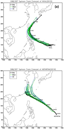
We chose 0000 UTC 7 May 2015 to demonstrate the singular vector perturbation evolution of Typhoon Noul because this typhoon made a right turn on 9 May 2015–10 May 2015. The singular vector ensemble members and the control forecast accurately predicted the right turn during this period. We selected 0000 UTC 3 July 2016 to demonstrate the singular vector evolution of Typhoon Nepartak because the CWBGFS model always proposed a northerly biased forecast for this typhoon and forecasts for Typhoon Nepartak were less accurate than those for Typhoon Noul. For these two periods, we found that if the control run was unable to produce an accurate forecast, then the ensemble members rarely yielded results dramatically more accurate in the ensemble mean. We were interested in differences between singular vectors in these two selected periods.

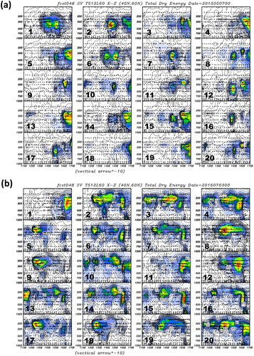
The horizontal structures of the singular vector perturbations are depicted by shading colour in Fig. 3, and contour lines show the 20 ensemble members as the geopotential height of 850 hPa. The initial time states are illustrated in Fig. 3a and b, and the positions of the TC are indicated by arrows in the first ensemble frame. The horizontal structures around the TC were similar to those in some theoretical studies (Fiorino and Elsberry, 1989; Li and Wang, 1994; Wang et al., 1998; Wang, 2002a, 2002b). In these studies, asymmetric circulations for wave number 1 or 2 (also called beta-gyres) interact with the TC symmetric flow and affect the subsequent movement and development of the typhoon. The horizontal asymmetric circulation scales around the TC in Fig. 3 are larger than those in theoretical studies. The largest amplitude was at approximately 200 hPa (not shown); this can be seen in the vertical cross-section figures (Figs. 4–6). Moreover, wave train structures were observed along the mid-latitude. They were singular vector perturbations from the calculation for the East Asia domain. Figure 3c and d present the 48-hour forecasts; the mid-latitude perturbations are greater than the TC perturbations. Especially in Fig. 3d (Typhon Nepartak), using the same shading scale to illustrate the TC and mid-latitude structures together causes the perturbations of some members around the TC to become unclear. We considered that the basic flow resolved by the CWBGFS model causes a northerly tendency in control trajectory forecasts. This basic flow for solving singular vectors indirectly causes northerly biases in active mid-latitude perturbations that are used to predict the majority of TC trajectories. Notably, Fig. 3c indicates that another tropical depression (approximately ${170}^{\circ }\mathrm{E},5^{\circ }\mathrm{N}$) followed Typhoon Noul but did not grow to become mature.

Fig. 3. Perturbations (shading) composed of two-domain singular vectors are added into the analysis to form 20 ensemble members (contour). The geopotential height (m) at 850 hPa are shown. (a) The 20 initial ensemble structures on 0000 UTC 7 May 2015. (b) The 20 initial ensemble structures on 0000 UTC 3 July 2016. (c) The 20 ensemble members of 0000 UTC 7 May 2015 after the 48-hour forecast. (d) The 20 ensemble members of 0000 UTC 3 July 2016 after the 48-hour forecast.

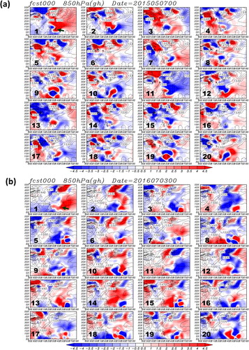
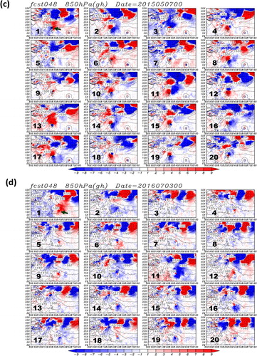
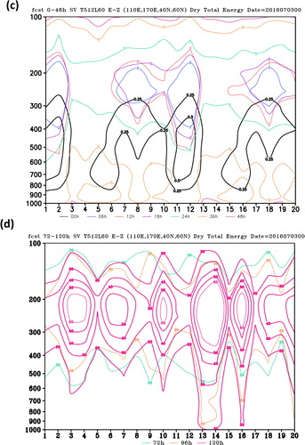
Fig. 4. Longitudinal-pressure dry total energy (J/kg) cross-sections of 20 members of singular vector perturbations. The longitude range is from $110°\mathrm{E}$ to $170°\mathrm{E},$ and the vertical range is from 1000 to 100 hPa. (a) At 0000 UTC 7 May 2015, the latitudinal average is taken from $5°\mathrm{N}$ to $25°\mathrm{N},$ (b) at 0000 UTC 3 July 2016, the latitudinal average is from $10°\mathrm{N}$ to $30°\mathrm{N}.$ The E-vector vertical component is 10 times of original.

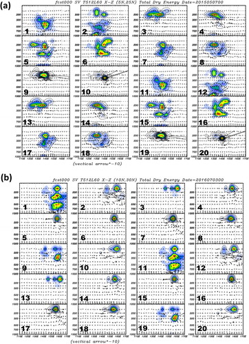
Fig. 5. As in Fig. 4 (a) For the 12-hour forecast of 0000 UTC 7 May 2015. (b) For the 24-hour forecast of 0000 UTC 3 July 2016.

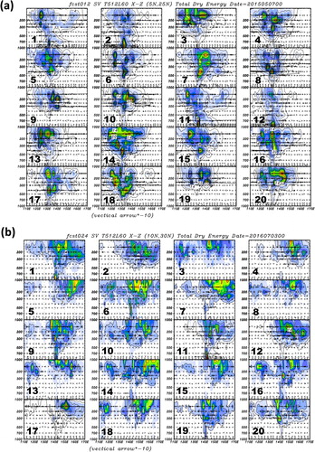
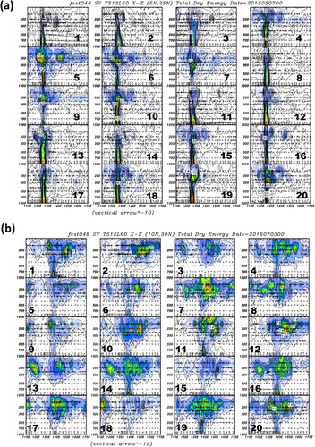
Fig. 6. As in Fig. 4 (a) For the 48-hour forecast of 0000 UTC 7 May 2015, the valid time on 0000 UTC 9 May 2015. (b) For the 48-hour forecast of 0000 UTC 3 July 2016, the valid for 0000 UTC 5 July 2016.

The vertical structure of the singular vector perturbation is shown in longitude and log-pressure cross sections based on the dry total energy. To illustrate perturbation structures around the TC, the latitudinal average was taken from $5°\mathrm{N}$ to $25°\mathrm{N}$ for Typhoon Noul and from ${10}^{\circ }\mathrm{N}$ to ${30}^{\circ }\text{N}$ for Typhoon Nepartak. The latitudinal averages of the two typhoons in the East Asia mid-latitude were taken from ${40}^{\circ }\mathrm{N}$ to ${60}^{\circ }\mathrm{N}.$ The longitude range in the cross-sectional figures was from ${110}^{\circ }\mathrm{E}$ to ${170}^{\circ }\mathrm{E}.$The arrows in the cross-sectional figures are x and p components of the three-dimensional (3D) E-vector. The 3D E-vectors (James, 1994) were calculated as follows: (5) $$\mathbf{E}=\left(\overline{{v^{\prime }}^2-{u^{\prime }}^2},-\overline{u^{\prime }{v}^{\prime }},-\frac{hf}{s^2}\overline{v^{\prime }{\theta }^{\prime }}\right)$$(5) where $$h(p)=\frac{R}{p}{\left(\frac{p}{1000\mathrm{ }\text{hPa}}\right)}^{R/C_p},\mathrm{ }{s}^2=-h(p)\frac{\partial {\theta }_R(p)}{\partial p}.$$

The E-vector is oriented in the direction of energy transport and $\partial \overline{u}/\partial t\propto \nabla \cdot \mathbf{E}.$

As shown in Fig. 4, the initial structures of the perturbation according to dry total energy were concentrated in the local areas and aligned vertically. Most members had clear structures in upper layers. In the 12-hour forecast for Typhoon Noul (Fig. 5a) and the 24-hour forecast for Typhoon Nepartak (Fig. 5b), the energy dispersed out of the initial area and formed the pillar structure. The E-vector (x, p) became horizontal, meaning that momentum flux dominated the perturbation development. In the 48-hour forecast (Fig. 6), all TC perturbations formed energy pillar structures. We concluded that upper layer perturbations mostly developed first and then induced growth in lower layer perturbations before finally forming pillar structures in the TC domains.

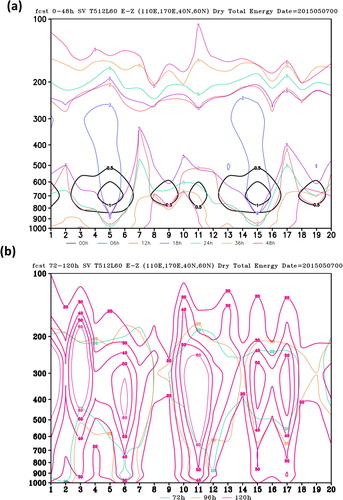
The initial and 48-hour-forecasted mid-latitude perturbations in dry total energy are presented in Figs. 7 and 8, respectively. The initial perturbations were located in the lower layers. The structures gained a westward tilt as the altitude increased. The E-vector exhibited an upward-oriented component ($\overline{v^{\prime }{\theta }^{\prime }}>0$). The 48-hour perturbations were concentrated in upper layers at approximately 200 − 300 hPa. These perturbations somehow maintained a westward tilt phase from 500 to 1000 hPa. The E-vectors exhibited significant horizontal components and the energy transport was dominated by momentum. The whole process in the mid-latitude was similar to a typical baroclinic instability in which perturbations are initiated in lower layers by temperature advection and then moved to higher layers through momentum flux (Hoskins et al., 1983).

Fig. 7. As in Fig. 4, but the mid-latitude singular perturbations are shown, and the latitudinal average is taken from $40°\mathrm{N}$ to $60°\mathrm{N}.$ (a) For 0000 UTC 7 May 2015. (b) For 0000 UTC 3 July 2016.

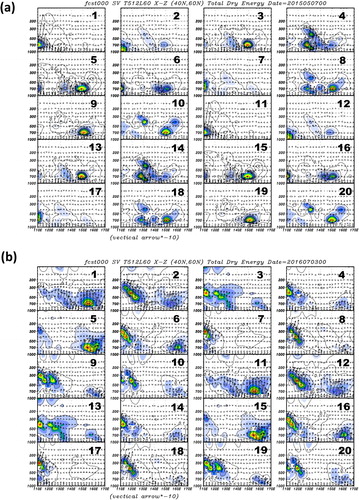
Fig. 8. As in Fig. 7, but the forecasts of the mid-latitude singular vector perturbations are shown. (a) For 48-hour forecast of 0000 UTC 7 May 2015, the valid time 0000 UTC 9 May 2015. (b) For 48-hour forecast of 0000 UTC 3 July 2016, the valid time 0000 UTC 5 July 2016.

3.2. Energy evolution of singular vector perturbations

We traced the evolution of dry total energy perturbations in the tropical and East Asia mid-latitude domains. Each domain covered 20 latitude and 60 longitude degrees. The energy was counted in this domain size to compare quantities in different ensemble members, areas, and counting domains. The contours in Figs. 9 and 10 illustrate the energy of singular vector perturbations in the two TC domains and the East Asia domain from the initial time to the 120-hour forecast. The horizontal axes of Figs. 9 and10 represent ensemble members, and vertical axes show vertical layers. The initial energy state is shown in black contours and the 120-hour forecast is shown in pink contours. Other time frames are traced by single contour values with corresponding colours. In Fig. 9a (Typhoon Noul), the initial energy (black contours) was located at approximately 200 hPa. Tracing the contour with a value of 5 over the 48-hour forecast time revealed the vertical downward energy dispersion. In the 72-to-120-hour forecast for Typhoon Noul (Fig. 9b), tracing the contour with a value of 10 revealed limited changes in energy states, and energy at the 120-hour forecast was at approximately 150 hPa. For Noul, the energy at approximately 150 hPa increased about two to three times in 120 hours. For Typhoon Nepartak (Fig. 9c and d), the initial energy was at approximately 150 hPa, and the value was smaller than the energy for Typhoon Noul. Tracing the contour for the value of 2 in Fig. 9c revealed a clear downward energy dispersion. In the 72-to-120-hour forecast for Typhoon Nepartak (Fig. 9b), we traced the contour for the value of 10; the energy slightly dispersed downward over time, and the 120-hour energy was at approximately 150 hPa. The energy at approximately 150 hPa for Typhoon Nepartak grew about 10 times in 120 hours, which was considerably higher than that for Typhoon Noul. However, the energy of the initial perturbations in Typhoon Nepartak was approximately one-fourth of the initial energy in Typhoon Noul.

Fig. 9. Evolution of perturbation dry total energy (J/kg) around tropical area in the 120-hour forecast. One contour is traced in different times, except the initial is shown in black contours and the 120-hour forecast is shown in pink contours. (a) The forecast is from the initial 0000 UTC 7 May 2015 to 48-hour. The value 5 is traced. (b) The forecast time is after (a) from 72-hour to 120-hour. The value 10 is traced. (c) The forecast is from the initial 0000 UTC 3 July 2016 to 48-hour. The value 2 is traced. (d) The forecast time is after (c) from 72-hour to 120-hour. The value 10 is traced.

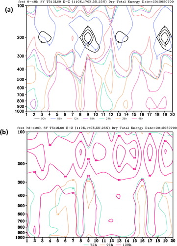
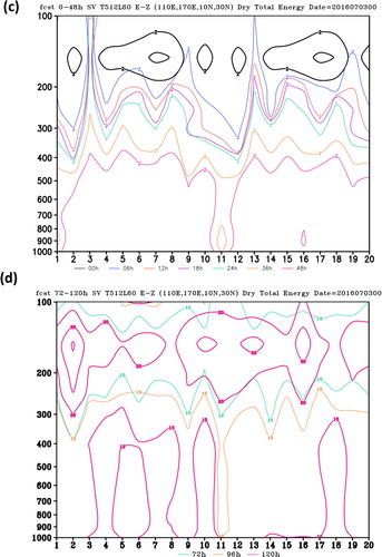
Fig. 10. As in Fig. 9, but the evolution of dry total energy around mid-latitude. (a) The forecast is from the initial 0000 UTC 7 May 2015 to 48-hour. The value 2 is traced in forecast < = 12-hour, and the value 5 is traced > = 18-hour. (b) The forecast time is after (a) from 72-hour to 120-hour. The value 20 is traced. (c) The forecast is from the initial 0000 UTC 3 July 2016 to 48-hour. The value 2 is traced < = 12-hour, and the value 5 is traced > = 18-hour. (d) The forecast time is after (c) from 72-hour to 120-hour. The value 20 is traced.

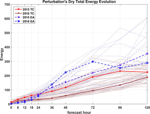
The corresponding East Asia mid-latitude perturbations are shown in Fig. 10. The initial mid-latitude singular vector perturbations were less than those in the TC domain. The initial energy structures of Typhoon Noul were located in the lower layers at approximately 700 hPa (Fig. 10a), and then, energy increased over time when we traced the contours with values of 2 (≤12 hours) and 5 (≥18 hours). In the 72-hour to 120-hour forecast (Fig. 10b), the significant energy areas moved to upper layers at approximately 300–400 hPa. The perturbation energy grew at least 60 times in 120 hours. The initial energy structures of Typhoon Nepartak were vertically extended (Fig. 10c), and the maximum areas were located in the range from 400 to 700 hPa. The energy mostly grew upward over time when we traced contours with values of 2 (≤12 hours) and 5 (≥18 hours). In the stage from the 72-hour to 120-hour forecast (Fig. 10d), significant energy areas moved to upper layers at approximately 200 − 300 hPa. For the TC and East Asia domains of both cases, we found that the perturbation growth did not follow the order of EVs from the energy norm calculation in the tangent and adjoint models. The perturbations from small EVs grew as quickly as those from large EVs. Moreover, the negative singular vector perturbations grew at least as quickly as the positive singular vector perturbations. The time dependence of the singular vector perturbations for dry total energy in the two cases for the TC and East Asia domains are shown in Fig. 11. The ensemble means of the energy in the TC domain are represented by red lines, those in East Asia domain are represented by blue dashed lines, and all the ensemble members are depicted by grey lines (TC domain: solid, East Asia domain: dashed). When checking the ensemble means for energy, we noticed that initial energy in the East Asia domain was less than that in the TC domain; however, at the 120-hour forecast, the energy in the East Asia domain was higher than that in the TC domain. The energy of some members, especially those in the East Asian domain, had become twice as high as the ensemble means at the forecast 120-hour.

Fig. 11. Time dependence of perturbation’s dry total energy (J/kg) for two cases in terms of both TC and East Asia domains. The total energy ensemble means of the TC domain (red solid lines) and East Asia domain (blue dashed lines) are shown. All the energy variations of ensemble members are indicated by grey solid lines (the TC domain) and grey dashed lines (East Asia domain).

4. Results of the transient eddy in analysis data

The pillar structures of singular vectors for energy in the TC domain formed after 12 − 24 hours, with a clear westward tilt and with an increase in height accompanied with upward E-vectors in the East Asia mid-latitude area. We examined analysis data to identify transient eddy structures and evolutions similar to singular vector perturbation structures and development processes. A transient eddy is defined as the variable value at a specific time subtracted from its monthly time series mean. We used Equation (2)(2) $$〈{\mathbf{x}}^{\mathbf{\prime }}(t_f),\mathbf{E}{\mathbf{x}}^{\mathbf{\prime }}(t_f)〉={\int }_D^{}{\int }_0^1\frac{1}{2}({u^{\prime }}^2+{v^{\prime }}^2)+\frac{1}{2}\frac{C_p}{\overline{T}}{T^{\prime }}^2\mathit{\text{dσdD}}+{\int }_D^{}\frac{1}{2}{R}_a\overline{T}\frac{{p^{\prime }}_s^2}{{\overline{p}}_s^2}dD.$$(2) to obtain the transient eddy dry total energy and employed Equation (5) to calculate the E-vector. When we checked the evolution of the transient eddy energy around the TC domain, similar processes were observed at the TC genesis stage (different dates with singular vector cases) and the self-reinforcement stage. In the East Asia domain, we easily found similar upward E-vector processes.

We noticed that the transient eddy energy began to move downward at approximately ${145}^{\circ }\mathrm{E}$ in the TC domain for Typhoon Noul (Fig. 12a) on 1800 UTC 2 May 2015, which was during the tropical depression stage. Considerable energy was concentrated in the top layers at approximately 100 − 200 hPa. The x and p components of the corresponding E-vector were oriented downward at approximately ${150}^{\circ }\mathrm{E}$ and 200 − 700 hPa (Fig. 12d). High transient eddy energies were always accompanied with clear $\nabla \cdot \mathbf{E}<0$(blue dashed contour) or $\nabla \cdot \mathbf{E}>0$ (red solid contour) phenomena. $\nabla \cdot \mathbf{E}>0$ implied accelerating westerly wind, and $\nabla \cdot \mathbf{E}<0$ indicated accelerating easterly wind. The TC circulation centres (vorticity maxima centres) with respect to altitude were always between $\nabla \cdot \mathbf{E}<0$ and $\nabla \cdot \mathbf{E}>0$ and were marked with a thick black dashed line. These centers were located in these regions because, in contrast to the southern and northern parts of the TC centre, the approximated circular circulation of the TC was always within the area indicated by $\nabla \cdot \mathbf{E}<0$ and $\nabla \cdot \mathbf{E}>0.$ However, in the latitudinal average of the cross-sectional figure, the convergent and divergent parts of $\nabla \cdot \mathbf{E}$ cancelled each other out. Therefore, $\nabla \cdot \mathbf{E}$ was lower near the TC centre than in ambient areas.

Fig. 12. Structures of transient eddy dry total energy (J/kg) in analysis data are shown in longitude-pressure cross section. The latitudinal average is from $5°\mathrm{N}$ to $25°\mathrm{N}$ for Noul’s case. (a) 1800 UTC 2 May 2015, (b) 1800 UTC 3 May 2015, and (c) 0000 UTC 7 May 2015. The corresponding E-vector (x, p) components (arrow) and $\nabla \cdot \mathbf{E}$(contour) are shown in (d), (e), and (f). The thick dashed line marks the centre of the TC.

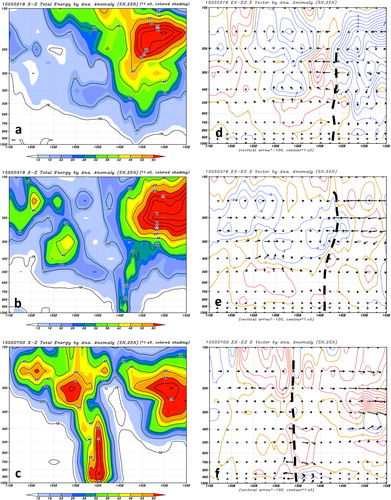
On the formation date of Typhoon Noul, at 1800 UTC 3 May 2015 (Fig. 12b and e), the transient eddy energy tilted eastward with altitude and the pillar structure formed. The E-vectors were oriented downward in areas located at approximately $140°\mathrm{E}-145°\mathrm{E}$ and 300–700 hPa. The downward energy propagation appeared to the east of Typhoon Noul’s centre. For 0000UTC 7 May 2015, which was the same date used for the singular vector perturbations (Fig. 4a), the TC transient eddy energy pillar structures were separated into two parts: one from 300 to 1000 hPa at approximately ${135}^{\circ }\mathrm{E}$ and another from 200 to 300 hPa at approximately ${128}^{\circ }\mathrm{E}$ west of the lower TC centre (Fig. 12c). The vertical alignment of the transient energy appeared to be composed of singular vector perturbations. That is, we could use the first six singular vector perturbations in Fig. 4a to determine the transient eddy energy in Fig. 11c. In Fig. 11f, the E-vectors indicated an upward energy orientation in lower layers (800–1000 hPa) east of the TC centres. We also noticed another significant energy area and clear E-vector components in upper layers east of the centres at approximately $150°\mathrm{E}-155°\mathrm{E}.$

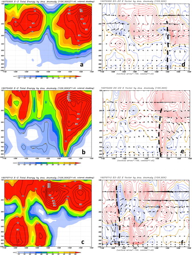
For Typhoon Nepartak (Fig. 13a), at 0000 UTC 3 July 2016, we observed significant areas of transient eddy energy in upper layers, which were the same as the singular vector perturbation calculations (Fig. 4b). The TC circulation was unclear at altitudes higher than 500 hPa on this date. The corresponding E-vectors (Fig. 13d) exhibited downward components east of the TC centres (thick dashed line) at approximately ${145}^{\circ }\mathrm{E}-{155}^{\circ }\mathrm{E}$ and 400 − 600 hPa. At 0000 UTC 4 July 2016, the transient eddy energy formed a pillar structure (Fig. 13b) and the E-vector exhibited downward propagation east of the TC centres. For 1200 UTC 7 July 2016, the typhoon was in its self-reinforcement stage, and the transient eddy energy formed two pillar structures. The E-vectors around these pillar structures also featured large horizontal and vertical components. The downward E-vector components appeared west of the TC centres and the upward E-vectors appeared east of TC centres.

Fig. 13. As in Fig. 12, but for Nepartak’s case. The latitudinal average is from $10°\mathrm{N}$ to $30°\mathrm{N}.$ (a) 0000 UTC 3 July 2016, (b) 0000 UTC 4 July 2016, (c) 1200 UTC 7 July 2016. The corresponding E-vector (x, p) components (arrow) and $\nabla \cdot \mathbf{E}$(contour) are shown in (d), (e), and (f). The thick dashed line marks the centre of the TC.

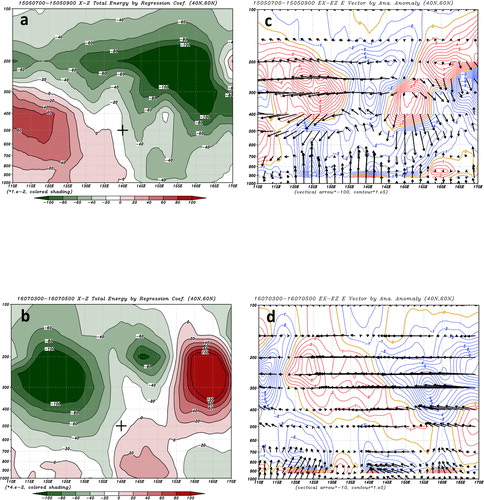
Figure 14 presents the mid-latitude transient eddy energy structures and E-vectors. We examined time averages for the periods of 0000 UTC 7 May 2015 − 0000 UTC 9 May 2015 and 0000 UTC 3 July 2016 − 0000 UTC 5 July 2016 because the mid-latitude transient eddy energies or E-vectors exhibited consistent results in these two time periods. In here, it was difficult to trace the single mid-latitude transient eddy as the TC transient eddy energies we followed in Figs. 13 and 14. To compare the results with mid-latitude singular vector perturbations, we used the one-point correlation (Lim and Wallace, 1991) method to demonstrate the transient eddy energy structures. The transient eddy dry energy one-point regression coefficients structures are shown in Fig. 14a and b. The specific one-point was selected at ($140°\mathrm{E},\mathrm{ }50°\mathrm{N},$ 500 hPa) and marked by a cross sign. The coefficient equation was the same as Lim and Wallace (1991). The structures had a slightly westward tilt with height, and the maximum values were approximately at 200 − 400 hPa, which are the jet stream positions. As to see the obvious westward tilt of transient eddy structures, the geopotential height can be selected in a one-point correlation analysis (Lim and Wallace, 1991). On the other hand, there were clear lower layer (700–1000 hPa) structures with upward-oriented E-vectors and $\overline{v^{\prime }{\theta }^{\prime }}>0,$ implying a westward tilt phase line with increasing altitude. During Typhoon Noul in 2015 (Fig. 13c), significant downward E-vectors were observed in middle layers at approximately 400–700 hPa. The contour areas delineated by $\nabla \cdot \mathbf{E}<0$ and $\nabla \cdot \mathbf{E}>0$ (Fig. 14c and d) were larger than those in tropical TC areas (Figs. 12 and 13). Therefore, the eddy scales of mid-latitude baroclinic systems were larger than those of tropical systems. Transient eddies could easily grow at lower layers with $\nabla \cdot \mathbf{E}<0.$ Then, transient eddies could return their energy back to the basic state in upper layers. In upper layers (200 − 300 hPa), the momentum $\overline{{v^{\prime }}^2-{u^{\prime }}^2}<0$ dominated and the E-vectors moved westward accompanied with large areas, where $\nabla \cdot \mathbf{E}>0,$ marked by the red contours. Therefore, the acceleration in the westerly wind and the basic flow received energy from transient eddies. Overall, the dynamic processes of mid-latitude transient eddies in the two typhoon periods were similar to those determined in previous studies.

Fig. 14. As in Fig. 12, but for the regression coefficients of the mid-latitude transient eddy dry energy. (a) The two days 0000 UTC 7 May 2015 − 0000 UTC 9 May 2015 average in Noul’s case, and (b) the two days 0000 UTC 3 July 2016 − 0000 UTC 5 July 2016 average in Nepartak’s case. The corresponding E-vector (x, p) components (arrow) and $\nabla \cdot \mathbf{E}$(contour) are shown in (c) and (d).

5. Conclusions and discussion

In this study, we compared the energy structures and the evolution of singular vectors and transient eddies (Table 2). We found that the mid-latitude singular vector perturbations always had consistent initial structures that essentially followed the baroclinic wave development process, as shown in many previous studies (Buizza et al., 1993; Buizza and Palmer, 1995; Palmer et al., 1998). These studies especially mentioned that the energies of singular vector perturbations are mainly transported from the lower to upper layers. However, we could not identify a suitable theory to explain singular vector structures in the TC domains. Ge et al. (2007, 2008) used an axisymmetric vortex to reveal that energy propagates downward from upper layers in resting and westerly vertical shear environmental flows. In their studies (Ge et al., 2007, 2008), TC structures had an upper anticyclone on the lower cyclone. By contrast, TC singular vector perturbations in the present study indicated barotropic modes (similar beta-gyre structures in the vertical direction) from 1000 to 100 hPa. In addition, we revealed that observational transient eddies in the TC area had this type of barotropic structure between 100 and 1000 hPa. Therefore, we focused on the perturbations of the TC circulation, whereas Ge et al. (2007, 2008) had discussed the Rossby wave dispersion around the TC vortex itself. The results of the present study (Figs. 5 and 6) did not indicate whether the wave trains around the TC in upper layers followed the process of Rossby wave dispersion. When Ge et al. (2010) used a real case to simulate the upper and lower interactions of the TC, they emphasised the effect of the Rossby wave train caused by the previous existing TC on the cyclogenesis of the subsequent new TC. The singular vector perturbations play roles in current existing TCs. The energy dispersion of perturbations or the energy of the TC itself should be evaluated in subsequent studies.

Table 2. The comparisons between singular vector and transient eddy.

	Initial horizontal structure of geopotential	Initial vertical structure of dry total energy	Energy evolution
singular vector in TC domain	beta gyre	irregular small round cell then forming pillar in 48-hour	upper layer development earlier than lower layer
singular vector in East Asia domain	cashew-nut	westward phase tilt	from lower layer to upper layer
transient eddy around TC area	irregular round or comma sign*	pillar or funnel	from upper to lower layer
transient eddy in mid-latitude	wave train*	wave train	lower layer upward middle layer downward

Note *: this structure is not shown in this article.

The singular vector perturbations in the TC domain and transient eddies around the TC area can be regarded as existing potential vorticity anomalies. We assumed a positive potential vorticity anomaly in upper layers at approximately 100–200 hPa. Then, according to the conservation of potential vorticity (Hoskins et al., 1997), the positive potential vorticity anomaly induced the corresponding upper and lower cyclonic circulation. Once those top–down cyclonic circulations combined together to form a pillar shape, they affected the development and movement of the TC. The results in Section 3 indicated that singular vectors in the TC domain were not located in lower layers because the horizontal temperature gradient and temperature flux ($\overline{v^{\prime }{\theta }^{\prime }}$) in lower layers were smaller than those in mid-latitude lower layers. Therefore, energy was transferred from the basic flow in upper layers through barotropic instability rather than from the basic flow in lower layers. However, this may have been caused by calculating dry energy without considering the effects of diabatic heating in lower layers. The top–down process was also noticed in observational transient eddy energy. The top–down process for transient eddy energy was observed in the TC precursor and the self-reinforcement stage of the TC. When considering the dry energy or the dynamic view, singular vector perturbations undoubtedly grew through one of the efficient dynamic processes. These perturbations were similar to horizontal beta-gyres, and they not only caused beta-drifts but also afforded the potential to gain energy from the basic flow. When upper perturbations or transient eddies formed, they could induce cyclonic perturbations in upper and lower layers.

According to Tam and Li (2006) and Li and Hsu (2018), the energy source of TCs in observational data revealed that the TC energy in formation processes is obtained from the eastern upstream. This upstream energy can be traced back to upper layers where $\overline{v^{\prime }{T}^{\prime }}<0.$ The upper layer energy was obtained from the equatorward momentum flux from mid-latitude where $\overline{u^{\prime }{v}^{\prime }}<0.$ However, these studies have focused on TC formation, with earlier stages than those we selected. The area upstream of the TC, the downward process in the tropical region, and the equatorward momentum from the mid-latitude area could all be studied using singular vectors.

The adiabatic process and dry total energy norm were considered to obtain singular vectors or for transient eddy analysis in the present study. That probably caused the incomplete information in singular vector perturbations in the TC domain and the insufficient explanation of transient eddy processes. Results provided by Lang et al. (2012) showed that significant differences between dry and moist singular vectors at their initial time are related to the potential energy in the upper layers (200 − 300 hPa). Ignoring the humidity perturbation and assuming that humidity is driven by dry perturbations in the fully nonlinear CWBGFS model, differences between humidity values in the control run and ensemble members must be studied in the future. In addition, resolving the adjoint model is crucial for resolving the fine structure of perturbation, moreover, this would lead to an explanation of some dynamic processes and improve ensemble forecasts. An adjoint model with a higher resolution will be assessed in future studies.

On the basis of the present study results, the amount and quality of observational data in TC upper layers should be increased or reassessed. More efforts are required to investigate the upper structures of ensemble perturbations, especially for TC trajectory prediction. Emanuel (2018) mentioned the importance of the upper outflow of the TC and its feedback. In addition, current ensemble data assimilation schemes may be improved by checking upper structures. Finally, we still require better dynamic theories or further developed numerical models to explain or simulate the downward dispersion of energy in the tropical area.

Acknowledgements

The authors appreciate the reviewer gave us good suggestions and pointed out the mistakes. We also thank the journal editor Dr. Nils Gustafsson for encouraging us to correct the mistakes and re-edit English writing. We want to thank our colleagues Mr. Deng-Shun Chen, Ms. Wen-Mei Chen, Dr. Jong-Gong Chern, Dr. Ting-Huai Chang and Dr. Jen-Her Chen for establishing the ensemble prediction system and the helpful discussions. Thanks Wallace Academic English editing, Mrs. Becky Meitin, and Mr. Harold A. Johnson III for correcting and editing our article.

Correction Statement

This article has been republished with minor changes. These changes do not impact the academic content of the article.

Appendix

Consider the linear operator L, which makes the initial time perturbation ${\mathbf{x}}^{\mathbf{\prime }}(t_0)$ to be final time perturbation ${\mathbf{x}}^{\mathbf{\prime }}(t_f)$ as follows: (A1) $$〈{\mathbf{x}}^{\mathbf{\prime }}(t_f),\mathbf{E}{\mathbf{x}}^{\mathbf{\prime }}(t_f)〉=〈\mathbf{L}{\mathbf{x}}^{\mathbf{\prime }}(t_0),\mathbf{EL}{\mathbf{x}}^{\mathbf{\prime }}(t_0)〉.$$(A1)

The L operator is a time forward operator and a tangent linear model in the singular vector calculation. By using the inner product identical equality, this equation can be rewritten as follows: (A2) $$〈{\mathbf{x}}^{\mathbf{\prime }}(t_f),\mathbf{E}{\mathbf{x}}^{\mathbf{\prime }}(t_f)〉=〈\mathbf{L}{\mathbf{x}}^{\mathbf{\prime }}(t_0),\mathbf{EL}{\mathbf{x}}^{\mathbf{\prime }}(t_0)〉=〈{\mathbf{E}}^{\mathbf{-}1}{\mathbf{L}}^{\mathbf{T}}\mathbf{E}\mathbf{L}{\mathbf{x}}^{\mathbf{\prime }}(t_0),\mathbf{E}{\mathbf{x}}^{\mathbf{\prime }}(t_0)〉,$$(A2) where ${\mathbf{L}}^{\mathbf{T}}$ is the adjoint operator. This equation connects the final and initial perturbation energies.

If (A3) $$\mathbf{K}\equiv {\mathbf{E}}^{-1}{\mathbf{L}}^{\mathbf{T}}\mathbf{E}\mathbf{L},$$(A3) then the EV ${\lambda }^2$ and eigenvector v can be described by (A4) $$\mathbf{K}v={\lambda }^{2}v.$$(A4)

Because the energy norm is used, the EV we use the square form. Next, using Equation (A4)(A4) $$\mathbf{K}v={\lambda }^{2}v.$$(A4) we obtain (A5) $$\begin{array}{c}{\Vert v(t_f)\Vert }^2=〈v(t_f),\mathbf{E}v(t_f)〉=〈\mathbf{K}v(t_0),\mathbf{E}v(t_0)〉\\ ={\lambda }^2〈v(t_0),\mathbf{E}v(t_0)〉\end{array}$$(A5) and (A6) $${\lambda }^2=\frac{〈v(t_f),\mathbf{E}v(t_f)〉}{〈v(t_0),\mathbf{E}v(t_0)〉}$$(A6)

The perturbation ${\mathbf{x}}^{\mathbf{\prime }}$ is composed of the eigenvectors v. The square norm (energy norm) is used here, so the EV ${\lambda }^2$ is associated with the singular value $\lambda ,$ with the eigenvector v as the singular vector. The eigenvector associated with the largest EV represents the fastest rate of growth. We can adopt the highest EVs and eigenvectors as optimal perturbations. Notice that because the matrix K is nonsymmetric, eigenvectors are nonorthogonal. Therefore, the number of eigenvectors is insufficient to cover the most unstable perturbations, and the eigenvectors cannot form a complete set. Thus, attempt to modify K into be symmetric matrix $\tilde{\mathbf{K}}$ by setting (A7) $${\tilde{\mathbf{x}}}^{\mathbf{\prime }}={\mathbf{E}}^{1/2}{\mathbf{x}}^{\mathbf{\prime }}.$$(A7)

Then, the original (A8) $$\mathbf{K}{\mathbf{x}}^{\mathbf{\prime }}={\lambda }^2{\mathbf{x}}^{\mathbf{\prime }}$$(A8) can be rewritten as (A9) $$\mathbf{K}{\mathbf{E}}^{-1/2}\widetilde{{\mathbf{x}}^{\mathbf{\prime }}}={\lambda }^2{\mathbf{E}}^{-1/2}\widetilde{{\mathbf{x}}^{\mathbf{\prime }}}$$(A9) and (A10) $${\mathbf{E}}^{1/2}\mathbf{K}{\mathbf{E}}^{-1/2}{\tilde{\mathbf{x}}}^{\mathbf{\prime }}={\lambda }^2{\tilde{\mathbf{x}}}^{\mathbf{\prime }}.$$(A10)

Then, by setting (A11) $$\tilde{\mathbf{K}}\equiv {\mathbf{E}}^{1/2}\mathbf{K}{\mathbf{E}}^{-1/2}={\mathbf{E}}^{1/2}{\mathbf{L}}^{\mathbf{T}}\mathbf{E}\mathbf{L}{\mathbf{E}}^{-1/2},$$(A11) we can notice that $\tilde{\mathbf{K}}$ is a symmetric matrix with the same EVs as K. The dimensions of matrix $\tilde{\mathbf{K}}$ are high, and we usually solve it by using the Lanczos method (Pissanetzky, 1984; Strang, 1986). Even if we cannot obtain all orthogonal eigenvectors by using the Lanczos method, we should still attempt to solve $\tilde{\mathbf{K}}$ rather than K because this ensures real EVs and orthogonal eigenvectors.

To calculate the specific area dry total energy at the final time, the norm for a specific area operator D can be defined as (A12) $$〈\mathbf{D}{\mathbf{x}}^{\mathbf{\prime }}(t_f),\mathbf{ED}{\mathbf{x}}^{\mathbf{\prime }}(t_f)〉.$$(A12)

D is the local projection proposed by Buizza (1994). We can easily derive the previous norm as (A13) $$\begin{array}{c}〈\mathbf{D}{\mathbf{x}}^{\mathbf{\prime }}(t_f),\mathbf{ED}{\mathbf{x}}^{\mathbf{\prime }}(t_f)〉=〈\mathbf{DL}{\mathbf{x}}^{\mathbf{\prime }}(t_0),\mathbf{EDL}{\mathbf{x}}^{\mathbf{\prime }}(t_0)〉\\ =〈{\mathbf{E}}^{\mathbf{-}1}{\mathbf{L}}^{\mathbf{T}}\mathbf{D}\mathbf{EDL}{\mathbf{x}}^{\mathbf{\prime }}(t_0),\mathbf{E}{\mathbf{x}}^{\mathbf{\prime }}(t_0)〉\end{array}$$(A13) and we can follow the same process from Equations (A10)(A10) $${\mathbf{E}}^{1/2}\mathbf{K}{\mathbf{E}}^{-1/2}{\tilde{\mathbf{x}}}^{\mathbf{\prime }}={\lambda }^2{\tilde{\mathbf{x}}}^{\mathbf{\prime }}.$$(A10) to (A14)(A14) $$\tilde{\mathbf{G}}={\mathbf{E}}^{1/2}\mathbf{G}{\mathbf{E}}^{-1/2}={\mathbf{E}}^{-1/2}{\mathbf{L}}^{\mathbf{T}}\mathbf{D}\mathbf{EDL}{\mathbf{E}}^{-1/2}.$$(A14) to obtain the following symmetric matrix: (A14) $$\tilde{\mathbf{G}}={\mathbf{E}}^{1/2}\mathbf{G}{\mathbf{E}}^{-1/2}={\mathbf{E}}^{-1/2}{\mathbf{L}}^{\mathbf{T}}\mathbf{D}\mathbf{EDL}{\mathbf{E}}^{-1/2}.$$(A14)