Multi-year ocean thermal variability

Abstract

Numerous indicators show that multi-annual and longer oceanic baroclinic variability retains a complicated spatial structure out to decades and longer. With time-averaging, the sub-basin scales connected to abyssal topography and meteorological structures emerge in the fields. Here, using 26-years of an oceanic state estimate (ECCO), an attempt is made to extract simpler patterns from the vertical average (whole water column) annual mean temperature anomalies and, separately, the vertical structures at each horizontal position. Singular vectors (SVs)/empirical orthogonal functions (EOFs) successfully simplify vertical and horizontal fields, but principal observation patterns (POPs) do not do so. About 3 horizontal spatial patterns account for more than 95% of the interannual and longer variances. A breakdown of the purely vertical structure at each grid point leads in contrast to an intricate variability with depth. Results have implications both for future sampling strategies, and for estimates, e.g. of the accuracy of any mean oceanic scalar.

Keywords:

• ocean variability
• ocean temperature

1. Introduction

The nature of low frequency (periods longer than a year or two) global ocean physical variability remains somewhat obscure with much of the difficulty lying with the observational data sets. Quasi-global coverage by altimetry is now almost 30 years long, but it depicts the surface elevation field – and whose interpretation reflecting motions at depth, including some troubling aliases, can be complex (Wang et al., 2013; LaCasce, 2017). The Argo float upper ocean (1–2 km) profile temperature field becomes nearly global about 15 years ago. Theoretical estimates of oceanic adjustment and variability time-scales (e.g. Wunsch, 2015, p. 338) cover a continuum at least out to 10,000 years and interpretations of the paleoclimate record support an hypothesis of change out to the entire age of the ocean (Cronin, 2010). The 20–30 year quasi-global record that does exist already raises some interesting questions about how to interpret it, and its implications for such common assumptions as the quantitative existence of a meaningful ‘climatological ocean’.

Common physical experience suggests that as the time scales of numerous natural phenomena increase, the spatial scale also increases. Implicit in many oceanographic studies is an assumption that as the high frequency ‘noise’ is averaged out over τ_avg, that the physics will simplify into the large-scale elements of the steady-state theories, perhaps being slowly time-dependent.

One difficulty is the implicit ambiguity in much oceanographic dynamical theory. Almost all useful and interesting theoretical circulation constructs (ranging from the thermal wind, through Sverdrup balance, Stommel-Arons flow, and the various thermocline theories) are written for a steady-state ocean in a laminar-like state (textbooks by Pedlosky (1996), Huang (2010), Vallis (2017), Klinger and Haine (2019), and others). The observed ocean is known to be filled with an intense, comparatively short-time-scale, turbulence-like motion having very strong spatial dependences in structure and time-scale. Apart from an extensive literature on the role of geostrophically balanced eddies (McWilliams, 2008), particularly as elements in parameterizations for mixing-like processes, little seems simple about the relationship between the physics of a hypothetical steady-state ocean, and one whose physical elements (velocity, temperature, pressure, etc.) have been averaged over a time-interval ${\tau }_{\mathit{avg}}>1$ yr. No spatial spectral-gap has ever been identified and no long-period cutoff is known, e.g. for time scales of the balanced (mesoscale) eddy field. All spatial and temporal scale interactions probably affect thermal variability patterns out to the longest accessible time intervals.

As global oceanic data sets and global general circulation models with quantifiable skill have emerged over the past few decades, the conclusion that the ocean has a very strong regional and temporal complexity has become inescapable. For example, Sonnewald et al. (2019), using a vertically integrated vorticity balance, divided the ocean laterally into 6+ distinct dynamical-type regions, of greatly varying area. Similarly, the altimetric wave number power-law results of Xu and Fu, 2012) seem to imply a minimum of about 14 dynamical regimes; cf. Hughes and Williams (2010). Sverdrup et al. (1942) identified 45 distinct topographic districts based upon the bathymetry known at that time.

An increasing complexity with averaging time, τ_avg, is readily rationalized: as τ_avg grows, the high-frequency, high-wavenumber variability that dominates the flow fields is further suppressed, permitting the zero-frequency structures of continental boundaries, bottom topography, and large-scale long-lived spatial inhomogeneities in air-sea exchanges, to emerge. Disturbances such as those owing to the mid-ocean ridges do not diminish with time, but can be manifested as strong spatial structures in both the mean and low-frequency variability over τ_avg.

Upper ocean variability over decades is comparatively well-observed, including the ENSO cycle, and sea surface temperatures, although problems persist (e.g. Chan et al., 2019). For the heat uptake estimation context, see the reviews by Abraham et al. (2013) or Meyssignac et al. (2019). In contrast, the goal here is to discuss the nature of full water-column low-frequency variability and its seemingly intricate spatial structure. Fields known to satisfy basic conservation equations as well as a very wide-variety of data, both meteorological and oceanographic are used (see Zanna et al., 2019) for discussion of the full-water column over a much longer time interval, and Wunsch, 2016). Much of what follows is descriptive, and is intended as an experiment in the depiction of decadal global variability using much-reduced volumes of values – and such that the result is comprehensible. The focus here is on the apparent spatial structures consistent with dynamics known from a self-consistent general circulation model and the diverse data, avoiding the issues forcefully raised by Bengtsson et al. (2004).

2. The estimated state

As a provisional estimate of oceanic variability and its average, we use the ECCO version 4 release 4 (v4r4) ‘state-estimate’ as documented by Fukumori et al. (2017, 2018, 2019) in the 26-year period 1992–2017. This depiction comes from a nonlinear weighted least-squares fit of the MITgcm (Marshall et al., 1997) and its evolutionary ECCO successors, to the diverse near-global data sets and meteorological forcing estimates that became available during and after the World Ocean Circulation Experiment. The single most important feature of this representation is that the model is free-running, but with its numerous control parameters having been previously adjusted so that the model trajectory takes it through all of the data points within (mostly) estimates of their uncertainties. The state estimate is represented on a geographical grid of $6.4\times {10}^6$ positions, including 50 different vertical layers; 26-yearly averages raises that number to $1.7\times {10}^8$ grid values. As the references make clear, the system includes a variety of parameterizations including those for the effects of the unresolved eddy field, and the special physics of the surface layer. Although the reliability of these parameterizations has been and continues to be much debated, the use of 26 years of data leads to adjustments in the parameters so that the state vector reproduces within estimated errors (a difficult subject in itself), the great bulk of the global data sets.

The free-running configuration is important because the results then satisfy basic global conservation of mass, energy, vorticity, etc. up to numerical accuracy – a feature not generally true of estimates commonly labelled ‘reanalyses’ (Bengtsson et al., 2004). Adjusted control parameters include the initial state, the meteorological forcing/coupling fields, and interior values of parameterized mixing rates. In terms of volume of data, the result is dominated by altimetry, Argo float profiles, instrumented elephant seals, and 6-hourly meteorological reanalysis products, all weighted by estimated errors. In contrast with earlier decades, by 1992 the observation system had become qualitatively more homogeneous and dense – reducing the tendency for changing observation methods and patterns to produce artifacts in the state. Direct observation of the deep ocean (below about 2000 m) remains very thin, and the values calculated here rely heavily on the known physics in the model connecting the upper and lower oceans while still accounting for whatever deep CTD temperature and salinity data that are available. References should be consulted for a full discussion. Only the temperature field is described here – because it has serious climate-change implications, has the longest records albeit at scattered points, and is observationally relatively intuitive.

The state estimate includes the full global ocean including ice-covered regions, and spans the entire 26 years of the estimate. (Comparisons – not shown – with an earlier 20-year climatology, omitting first and last years, and using only latitudes equatorward of 60° Fukumori et al. (2018) showed only small changes in the results.) Annual averages, which suppress much high frequency variability, including the spatially complicated annual cycle of temperature, are used as a first-step in reducing the volume of numbers required to describe the ocean – a significant reduction compared to a 1-hour or smaller model time-step. A second major data volume reduction is obtained by working with the column average annual temperatures – an unorthodox variable, but nonetheless one describing a major variability aspect.

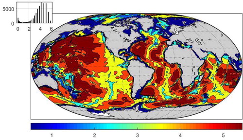
Figure 1 shows the model topography, whose numerous deep sub-basins are readily apparent, each having a physics determined by details such as proximity to large-scale boundaries, topographic slopes, presence of bottom roughness, latitude, structure of meteorological exchanges, etc. and which can be expected to generate full water column disturbances, not necessarily localized, as averaging periods increase.

Fig. 1. Bathymetry of the model (km) at 1 km intervals. As the deep ocean influences the thermal structure with increasing duration, the complex geometry of the topography can be dominant in the physics dividing the ocean into a large number of regionally distinct places. Compare to Sverdrup et al. (1942, Plate 1). Inset here and in other figures is a histogram of the plotted values.

Fourier spectra in space and/or time have proved in many ways to be the most productive representation of geophysical variability. An approach to the frequency-wavenumber spectrum was described by Wortham and Wunsch (2014). On the other hand, such descriptors are most powerful when fields are statistically stationary (in the ‘weak-’ or ‘wide’-sense), that is homogeneous in space and time. In the present situation, the spatial inhomogeneity is so strong that the estimated Fourier results are not discussed. Temporal non-stationarity is less obvious, but the trend-like behavior seen below in some elements would suggest that it is present as well.

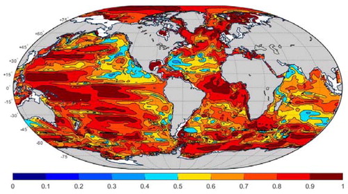
The nature of the temperature field can be seen from the 1994 potential temperature average shown in Fig. 2 for 477 m and its temporal standard deviation in Fig. 3. That particular depth was chosen as a compromise generally lying below the mixed-layer, but above the main thermocline. As has been realized since oceanographic antiquity, little or no structure arising from the huge mid-ocean ridges and other topographic features can be perceived in the upper ocean levels. Apart from the continental margins, inferring topography from such a picture would fail. Inferences about large-scale wind structures are, however, possible. Determining an accurate spatial mean temperature from in situ measurements requires a large number of values, appropriately distributed, even were there no underlying temporal changes. Notice that at this depth, no particular excess variance is seen in the equatorial Pacific Ocean.

Fig. 2. Average potential temperature (not the anomaly) at 477 m during 1994. Note the multi-modality of the values (inset).

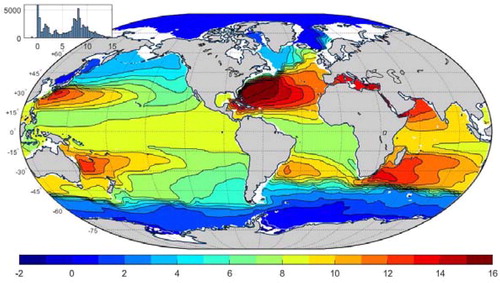
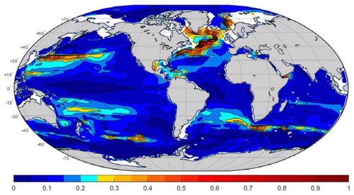
Fig. 3. Standard deviation (^oC) in time of annual mean temperature at 477 m over 26 years. Intricacy of the northern North Atlantic is apparent, as are the Kuroshio path, the region south of Cape Agulhas, and other ‘hot spots’. Spatial stationarity is an unattractive hypothesis.

3. Vertical average temperature

If $\varphi ,\lambda ,z,t$ are latitude, longitude, depth and time respectively, the underlying field is potential temperature, $T({\varphi }_p,{\lambda }_q,z_r,t_m),$ on the model space-time grid where the subscripts are integers. The time mean vertical average temperature, ${\overline{T}}_G({\varphi }_p,{\lambda }_q),$ is depicted in Fig. 4, the overbar denoting the 26-year time average. Some visual covariance with the bottom topography appears, as expected, with shallow regions necessarily being warmer – absent the deep cold water (the point pattern-correlation is 0.25). Most of the rest of this paper explores the temporal structure of the vertically averaged temperature as an ocean descriptor – with the understanding that ultimately every point (varying with latitude, longitude, depth, and time) is likely quantitatively unique. The resulting standard deviation of annual values with depth in the global spatial average can be seen in Fig. 5, with its near-surface domination.

Fig. 4. Twenty-six year time-average of the vertical mean potential temperature (°C) in the ECCOv4r4 state estimate, ${\overline{T}}_G(\varphi ,\lambda ).$

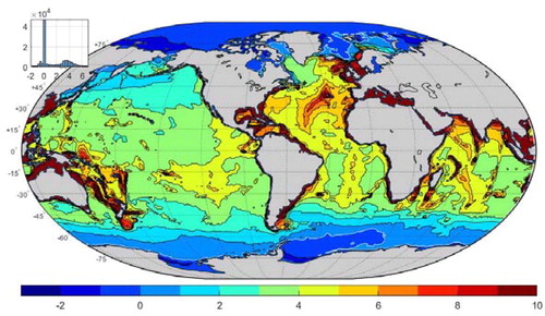
Fig. 5. Standard deviation (°C) for potential temperatures as a global average (a) and for the layer-thickness weighted values (b), m °C. Note use of the logarithmic scale for temperature alone. All model grid areas are given equal weight here.

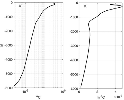
Water-column average temperature anomaly averaged also by year, $T_G({\varphi }_p,{\lambda }_q,t_m),$ where t_m is the year, is the present focus. T_G is interesting as being directly related to annual oceanic heat uptake, a subject not explored here. From the above references, the results below are expected to be dominated by the upper ocean, as indicated by the global average and time-depth variance of temperature (Fig. 5), noting however, that the upper ocean variability is partially compensated in the vertical average by the much-thicker model deep layers. (These particular values are not corrected for horizontal area changes in the state estimate model grid.) Vertical averaging also reduces the lateral inhomogeneity of the temporal variations.

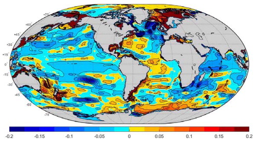
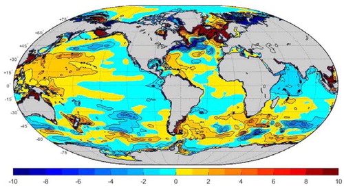
A qualitative sense of the spatial variability in latitude and longitude of the anomaly over the full water column through time can be seen in Figs. 6–8. Some effects of basin-scale topography are visible, particularly in the Atlantic, southeast Pacific, and western Indian Ocean. Particularly striking is the anomaly for 1998, the midst of an El Niño episode, with its intense equatorial features that are not apparent in the two other years shown. Space-time sampling requirements are visibly daunting. Some elements of these figures are associated with the abyssal topography, but any such effect is subtle, and the underlying dynamics is dependent not just upon the water depth, but also its two-dimensional gradients, at least.

Fig. 6. Anomaly of vertically integrated temperature for 1993, $T_G(\lambda ,\varphi ,t=1993)$ (°C).

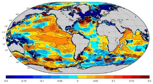
Fig. 7. Same as Fig. 6 except for 1998 – an El Niño year.

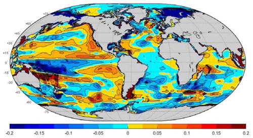
Fig. 8. Same as Fig. 6 except for 2017. An east-west basin divide occurs in the Atlantic Ocean.

4. Singular vectors, principal component analysis, EOFs, etc

Description and interpretation of any such field becomes an exercise in various forms of matrix decompositions. A brief discussion is provided below to obtain a notation and to lay out the necessary assumptions. Two of the best-known methods of reducing space-time patterns to the simpler representations are via principal oscillation patterns (POPs), and singular vectors (SVs), the latter often known as empirical orthogonal functions (EOFs) or principal component analysis (PCA). Both methods are fully described, e.g. by von Storch and Zwiers (2001). In practice here, only the second method proves to be effective at dimension reduction, and the POP discussion is consigned to the Appendix.

The three objects in the title of this section are basically the same. A singular value decomposition terminology will be used, as it appears to be the most nearly generic.¹ Textbook discussions can be found in Jolliffe (2002), Lawson and Hanson (1995), von Storch and Zwiers (2001), Wunsch (2006) and in Jolliffe and Cadima (2016), amongst others.

Consider any two dimensional matrix M where each column represents variations over space coordinates, and with time varying between columns, e.g. ${\mathbf{M}}_r(\mathbf{r},t).$ The subscript r is used to show that the position, $r_j,$ is an element of a vector, rather than being, e.g. latitude, and longitude separately as in M. Using the Eckart-Young-Mirsky theorem, (1a) $${\mathbf{M}}_r\left(\mathbf{r},t\right)={\mathbf{U}}_r\left(\mathbf{r}\right){\mathbf{\Lambda }}_r{\mathbf{V}}_r{\left(t\right)}^T=\sum _{j=1}^{K=26}{\lambda }_{rj}{\mathbf{u}}_{rj}\left(\mathbf{r}\right){\mathbf{v}}_{rj}^T\left(t\right)$$(1a) (1b) $${\mathbf{U}}_r=\left\{{\mathbf{u}}_{rj}\right\},{\mathbf{V}}_r=\left\{{\mathbf{v}}_{rj}\right\},{\mathbf{\Lambda }}_r=\mathit{diag}\left\{{\lambda }_{rj}\right\}$$(1b) exactly, where the elements of the diagonal matrix ${\mathbf{\Lambda }}_r$ are the singular values, ${\lambda }_{rj}.$ Maximum dimension, K, is less than or equal to the smaller of the number of rows and columns in ${\mathbf{M}}_r$ (in this paper, maximum dimension (rank) is limited by the number of years used, K = 26). Each column, ${\mathbf{u}}_{rj}$ of the K × K orthogonal matrix ${\mathbf{U}}_r$ varies with the geographical location.² Columns, ${\mathbf{u}}_{rj},$ are readily remapped back to ordinary geographical space. Each column, ${\mathbf{v}}_{rj},$ of the $K\times K$ orthogonal matrix ${\mathbf{V}}_r$ is the time-history of the particular spatial pattern in ${\mathbf{u}}_{rj}.$ All vectors have a norm of 1 and the units of ${\mathbf{M}}_r$ are in ${\mathbf{\Lambda }}_r.$ (Because the SVD is used in several different ways here, Table 1 lists the differing labels.)

Table 1. Notation used when applying the SVD to differing fields. Singular vectors are all functions of a geographic coordinate, or of time.

SVD notation	Field	Dependence
${\mathbf{u}}_{rj,}{\lambda }_{rj},{\mathbf{v}}_{rj}$	Generic in space	Space coord., arbitrary field, arbitrary field
${\mathbf{u}}_{Tj,}{\lambda }_{Tj},{\mathbf{v}}_{Tj}$	Vertical temperature	Depth, temperature, time
${\mathbf{u}}_{dj,}{\lambda }_{dj},{\mathbf{v}}_{dj}$	Vertical thickness weighted	Depth, temperature × layer-thickness, time
${\mathbf{u}}_{Gj,}{\lambda }_{Gj},{\mathbf{v}}_{Gj}$	Global vert. avg. temperature	Latitude/longitude, Temperature, time

Useful extensions of singular vector analyses are possible, including application in the frequency domain. For example, Wills et al. (2018) discuss separating atmospheric patterns by forcing decoherence of large-scale variability. They did however, employ a 114-year long record, something far beyond what is oceanographically available.

5. Vertical structures

Before describing the results for the vertically integrated field, it is useful for the reader to recognize some of the vertical structures that are being suppressed by integration and subsequently ignored. At each lateral position $r_j,$ the potential temperature anomaly is a two-dimensional matrix of depth and year, $T(r_j,z_k,t_p),$ with a singular value decomposition, (2) $$T\left(r_j,z_k,t_p\right)=\sum _{q=1}^{25}{\lambda }_{Tq}{\mathbf{u}}_{Tq}\left(r_{j,}{z}_k\right){\mathbf{v}}_{Tq}{\left(r_{j,}{t}_p\right)}^T,$$(2) and is different for every horizontal grid point. K = 25 because the vanishing temporal mean reduces the degrees of freedom by 1 from the 26 years available. Here, position r_j is only parametric in the SVD with the independent variables being depth and time. Anomalies are calculated relative to the time-mean at each point and depth. Note the similarity to the results of Pauthenet et al. (2019), but with their analysis is confined to the upper ocean and including salinity changes.

The SVD is here applied to the layer-depth-weighted potential temperature anomalies, a weighting that much reduces the vertical variance changes (Fig. 5) without removing it altogether. SVD elements are labelled ${\mathbf{u}}_{dj},$ etc. Because temperature structures in the near-surface boundary layer are dynamically distinct, the depth range in Eq. 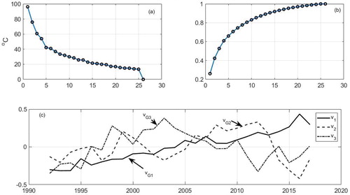(2)(2) $$T\left(r_j,z_k,t_p\right)=\sum _{q=1}^{25}{\lambda }_{Tq}{\mathbf{u}}_{Tq}\left(r_{j,}{z}_k\right){\mathbf{v}}_{Tq}{\left(r_{j,}{t}_p\right)}^T,$$(2) is applied only to the region below the 10th layer, 105 m and greater. Fig. 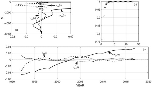5 shows the global average singular values as well as the fraction of the global average variance in each ${\lambda }_j^2/{\sum }_{q=1}^{25}{\lambda }_q^2.$ In the global median, the first three singular vectors describe more than 95% of the vertical variance – although the nature of those singular vectors varies widely over the ocean. Their global means, denoted by a bracket, $〈·〉,$ are shown in Fig. 9. A quasi-linear trend is visible in $〈{\mathbf{v}}_1(t_p)〉$ representing an overall trend (net warming) in this mode. The corresponding $〈{\mathbf{u}}_{d1}(z)〉,$ truncated in the figure, reaches a maximum at a depth of 300 m. But note that even so, a non-negligible cooling exists at depth both in this and other modes. A sign convention has been imposed such that a positive near-surface (105 m) value in ${\mathbf{u}}_{dj}(z_p)$ corresponds to a warming when the corresponding ${\mathbf{v}}_{dj}(t_p)$ is increasing.

Fig. 9. (a) Global mean of first 3 vertical singular vectors. u ${}_{d1}(z)$ reaches 0.1 at a depth of 300 m and the plot is truncated for visibility. (b) Shows the accumulated variance in each global median ${\lambda }_{di}^2$ normalized to sum to 1. Roughly speaking, the lowest SVD carries about 75% of the variance and the first 3 represent over 95% of the variance. (c) Shows the first 3 ${\mathbf{v}}_{d1}(t).$

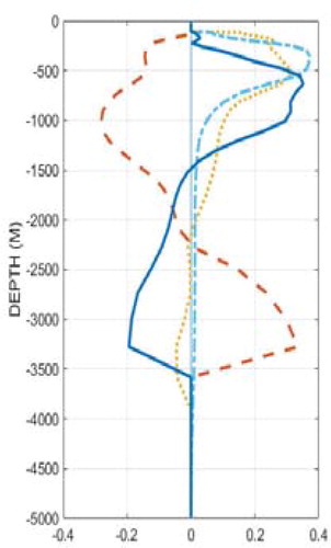
To show the variety of lowest modes, Fig. 10 depicts a sampling along 180° W in the Pacific Ocean. Vertical structures vary from having no zero crossings to having two or more.

Fig. 10. The lowest singular vector ${\mathbf{u}}_{d1}$ at a variety of latitudes along 180° W (dimensionless). Greatest depths do not exist for these particular positions.

Let n_z denote the number of zero-crossings in ${\mathbf{u}}_{d1}$ below 100 m. If $n_z=0,$ temperature change is of one sign with depth, and might be associated with a simple vertical heave or with the first linear baroclinic mode, although such an association is a very loose one. Similarly, $n_z=1,$ might be associated with the 2nd linear baroclinic mode, with one sign change with depth.

Fig. 11 displays the histograms of the number of zero crossings in all of the singular vectors, and of the number of zero-crossings in ${\mathbf{u}}_{d1}$ alone. The most common mode is that with no zero-crossings, and it constitutes approximately 40% of the lowest mode. That is, about 40% of the ocean area is described (insofar as the corresponding ${\lambda }_{d1}$ dominates) by a pure vertical heave of the isotherms (see the discussion in Bindoff and Mcdougall, 1994). But globally, the structure is vertically very complicated in these terms, likely because of the large variety of topographic interaction physics. Fig. 12 shows the horizontal distribution of the variance accounted for by the lowest SVD pair, ${\lambda }_{d1}{\mathbf{u}}_{d1}{\mathbf{v}}_{d1}^T,$ with the caveat that the structure of ${\mathbf{u}}_{d1}$ varies spatially. Apart from the eastern North Pacific, the western North Atlantic and the southern Indian Ocean, the lowest pair, of differing structures, accounts for 50% or more of the variability. An explanation of why those regions appear exceptional is not attempted here. Even there at least 40% of the variability is accounted for.

Fig. 11. (a) Fraction of the number of zeros occurring in all vertical modes ${\mathbf{u}}_d.$ (b) Fraction of the number of zeros occuring only in the lowest mode ${\mathbf{u}}_{d1}.$

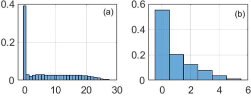
Fig. 12. Fraction of the vertical variance at each point in the lowest singular vector ${\mathbf{u}}_{d1}$ (dimensionless). It is, in general, not the same as a linear dynamical mode, but contains extra structure (zero crossings in the vertical).

6. SVD of vertical average temperature

Now mapping ${\varphi }_i,{\lambda }_k$ onto a two-dimensional vector position, r_j, the result, ${\overline{T}}_G$ ${}_r(r_j,t_p),$ is a matrix with averages over a time-interval of 1 year. Water-column average potential temperatures anomalies relative to the overall 26-year time mean are computed at each grid point with each matrix column defining those temperatures at all lateral locations at one time, t_p. Fig. 13 displays the ordered squared singular values and their normalized sum squared from the water depth average anomalies. Evidently, reproducing 90% of the space-time variance of ${\overline{T}}_G$_r requires of order 13-orthogonal patterns, with moderate domination of the lowest vectors. As many references remind readers (e.g. von Storch and Zwiers, 2001, p. 294), the singular vectors do not necessarily have any dynamical mode significance, whereas the POPs (Appendix), can.

Fig. 13. (a) Global median singular values λ_Gj (°C) and their normalized cumulative sum (b). (c) Shows the mean temporal coefficients ${\mathbf{v}}_{Gj}(t)$ for $j=1,2,3.$

Patterns of the first 3 ${\mathbf{u}}_{Gi}$ are displayed in Figs. 14–16. Here the strongest pattern, accounting for about 25% of the 26-year variance, has a time dependence, ${\mathbf{v}}_{G1}(t)$ that is dominated by an overall visual near-straight line trend. It corresponds to the similar behavior of ${\mathbf{v}}_1(t)$ The same convention is made here that positive regions of ${\mathbf{u}}_{Gi}(\varphi ,\lambda )$ increase (warm) with increasing ${\mathbf{v}}_{Gi}(t)$ and corresponding negative regions decrease. The North Atlantic produces the most complex response, with strong cooling adjacent to strong warming including the Gulf of Maine region (e.g. Piecuch et al., 2017). Evidently, the global pattern of full-water column temperature change, while quasi-linear in time, is made up of the difference between large-area cooling and warming regions. ${\mathbf{u}}_{G2}(\varphi ,\lambda ){\mathbf{v}}_{G2}{(t)}^T$ has a maximum following the 1997–1998 El Niño event, with an equatorial structure strongest in the western Pacific Warm Pool, but one also connected to a global pattern of change. That and the 3rd singular vector (Fig. 16) also contain major elements in the northern North Atlantic, supporting an hypothesis that the intricate changes there are the result of several different physical mechanisms and consistent with the complexity of the interannual changes in Figs. 6–8.

Fig. 14. Structure of 1000${\mathbf{u}}_{G1}$ mapped onto latitude and longitude (dimensionless). Sign change coincides with the yellow-blue boundary.

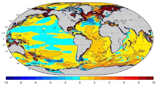
Fig. 15. $1000u_{G2}$ mapped onto latitude and longitude.

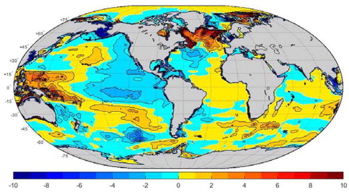
Fig. 16. 1000${\mathbf{u}}_{G3}.$ Western tropical Pacific and high North Atlantic structures are notable.

That a net warming of the water column average temperature has occurred over 20+ years is no surprise (Meyssignac et al., 2019; and numerous others). Overall warming of the South Atlantic in ${\mathbf{u}}_{G1}$ is striking. Note the inference (e.g. Gebbie and Huybers, 2019) that considerable parts of the deep ocean are still cooling from long-ago meteorological changes, superimposed here on fluctuations from ordinary internal variability at all depths with mixed signs.

The use of a vertical average temperature anomaly mutes the known strong variability at fixed depths. ${\mathbf{u}}_{G3}$ (Fig. 16) does contain a long zonal feature near the equator in the Pacific Ocean – likely a small residual of the strong ENSO cycle manifest there in the upper ocean. On the other hand, ${\mathbf{v}}_{G2},$ the temporal coefficient of ${\mathbf{u}}_{G2},$ shows a clear maximum value during the ENSO episode of 1998. It too has an equatorial Pacific feature, although not conspicuously stronger there than elsewhere.

6.1. Uncertainties of the SVD

For singular vectors corresponding to nearly equal singular values, it is well-known that an instability exists of the detailed structures contained in the two sets of vectors. Thus, Jolliffe (1986, p. 39), the asymptotic properties of the singular values λ_i and ${\mathbf{u}}_{Gi}$ can be obtained if subject to a comparatively simple hypothesis about the statistical distribution of the field covariance, and then λ_i, ${\mathbf{u}}_i$ are normally distributed. When the results here were compared to those from a shorter 20-year interval (ECCOv4r3), changes were only slight.

7. Summary and discussion

An unorthodox use is made of the column-average vertical potential temperatures in the ocean to reduce the numerical volume, and thus describe the bulk ocean potential temperature variability over 26 years. These structures are computed from an energy, mass, etc. conserving state estimate. The state estimate used here is not truth: like any statistical best-estimate it has intrinsic stochastic and systematic uncertainties. Using singular vectors (SVDs or EOFs) requires about 13 globally uncorrelated vector pairs in the horizontal domain for the water-column vertical average temperature. The spatial structure vectors, ${\mathbf{u}}_{Gi},$ (notation defined in Table 1) markedly display the complex of time scales and structures of the northern North Atlantic – emphasizing the links between purely local and global-scale changes.

In the vertical domain, with a separately computed decomposition, a smaller number of uncorrelated vector pairs is required. Approximately 40% of the dominant (lowest) mode of vertical structure can be described as analogous to the zeroth dynamical mode (vertical heave), but overall vertical structures are complicated, in large-part probably because of the great variety of potential topographic interactions. An analysis of principal oscillation patterns, POPS, of the vertical mean potential temperatures (in the Appendix) is not successful in measurably reducing the number of required structures.

With extended duration, the geometry of oceanic boundaries, including the sea floor topography, and regional long-lived meteorological elements (e.g. regions of excess curl), begin to emerge from the background noise, giving rise to kinematically and dynamically distinct provinces. Analytic understanding of low-frequency thermal variability takes on a strongly regional character, while remaining embedded in, and subject to, larger basin and global scale changes. Results here for the northern North Atlantic Ocean, consistent with previous regional analyses, are a particularly clear example of geographical variation. Any dynamical assumption, implicit or otherwise, that the time-average ocean has a simplified large-scale behavior, needs to be justified observationally. The averaging time, τ_avg, required for that to be rigorously true, is likely much longer than 26 years, but whether it is 100 or 1000 years, or if it is valid at all, remains obscure and awaits either much longer observational records, or analysis of demonstrably skillful high resolution circulation models. Wunsch (2018) and Meyssignac et al. (2019) address some of the sampling issues associated with persistent spatial patterns in thermal fields. These consequences are not described here.

Acknowledgements

I had useful comments on an early draft from R. Ferrari. Comments from two anonymous reviewers led to a major re-write of the paper. Thanks to all the members of the ECCO Consortium and once again to Diana Spiegel for computational assistance.

Disclosure statement

No potential conflict of interest was reported by the authors.

Additional information

Funding

Work funded in part from the Jet Propulsion Laboratory, NASA Contract NNN12AA01C with MIT. Completed at home in the Trump pandemic.

Notes

1 Many other labels exist in a variety of other fields (e.g. Karhunen-Loève expansion; proper orthogonal decomposition).

2 Vectors, lower-case bold, $\mathbf{q},$ here are columns. The transposes, ${\mathbf{q}}^T,$ are row vectors. Matrices are upper case bold e.g. M.

3 The close linkage between covariance assumptions, e.g. in objective mapping methods, and assumptions about the underlying physics is often forgotten or ignored.

Appendix.

Principal observation patterns (POPs)

Following Hasselmann (1988), the extended account in von Storch and Zwiers (2001) and references there, consider the principal observation patterns (POPs) and which can have a closer relationship to the underlying dynamics than do the singular vectors. The singular vectors are able to extract covariances amongst the non-orthogonal POPs, and thus can sometimes greatly simplify the dominant patterns, but the forced orthogonality mixes the POPs in the singular vectors.

To sketch the machinery, consider any time-dependent model with a state vector, $\mathit{\xi }(t),$ and whose time-evolution can be represented in the general linear form (e.g. Wunsch, 2006), (3) $$\mathit{\xi }\left(t+\Delta t\right)=\mathbf{A}\left(t\right)\mathit{\xi }\left(t\right)+\mathbf{B}\left(t\right)\mathbf{q}\left(t\right).$$(3)

$\mathbf{A}(t)$ is the ‘state transition matrix’ and $\mathbf{B}(t)\mathbf{q}(t)$ is a generic representation of model forcing and error fields. In what follows, three strong, if possibly plausible, assumptions are made: (1) That the field of annual temperature anomaly is sufficiently weak that a linear evolution is accurate; (2) that the governing physics over 26 years are time-stationary such that $\mathbf{A}(t),\mathbf{B}(t)$ are time-independent, A, B; (3) that the external control $\mathbf{B}(t)\mathbf{q}(t)$ is a stochastic process in space and time, and not dependent upon $\mathit{\xi }(t).$ Here $\Delta t=1$ year and $\mathit{\xi }(t)=$ ${\overline{T}}_G$ ${}_r(t).$ The subscript r again is placed on ${\overline{T}}_G$ to indicate that it is mapped from latitude and longitude into a one-dimensional vector at each fixed time. Equation (3)(3) $$\mathit{\xi }\left(t+\Delta t\right)=\mathbf{A}\left(t\right)\mathit{\xi }\left(t\right)+\mathbf{B}\left(t\right)\mathbf{q}\left(t\right).$$(3) can be regarded as a generalization of an autoregressive process of order (1) that is, AR(1), but it is, in practice, a very general linear state vector representation.

None of these assumptions is rigorously correct: the state vector of the ECCO estimate includes temperature only as a subset of the full suite of variables describing the ocean circulation and not their vertical means; stationarity in time remains to be properly tested; the best characterization of $\mathbf{B}(t)\mathbf{q}(t),$ including meteorological variables, is more complicated than an unstructured random process unrelated to $T_r(t),$ and portions of the field are likely nonlinear. Using the temperature field as a state vector can be at least partially justified through the thermal wind equations and the dependence of the geostrophic adjustments on temperature (density).

Consider the product of Eq. (3)(3) $$\mathit{\xi }\left(t+\Delta t\right)=\mathbf{A}\left(t\right)\mathit{\xi }\left(t\right)+\mathbf{B}\left(t\right)\mathbf{q}\left(t\right).$$(3) with $\mathit{\xi }{(t)}^T$ and with a bracket denoting expectation: (4) $$〈\mathit{\xi }\left(t+\Delta t\right)\mathit{\xi }{\left(t\right)}^T〉=\mathbf{A}〈\mathit{\xi }\left(t\right)\mathit{\xi }{\left(t\right)}^T〉+〈\mathbf{Bq}\left(t\right)\mathit{\xi }{\left(t\right)}^T〉,\mathrm{ }\text{or}$$(4) (5) $$\mathbf{R}\left(\Delta t\right)=\mathbf{AR}\left(0\right)$$(5) where $\Delta t$ is a nominal time-step which in the raw GCM is less than 1 hour, but here will be taken as 1 year. (This choice corresponds to a strong assumption that high frequency motions act only through $\mathbf{Bq}(t).)$ Expectation is over a hypothetical ensemble of oceanic states.

A can thus be obtained as (6) $$\mathbf{A}=\mathbf{R}\left(\Delta t\right)\mathbf{R}{\left(0\right)}^{-1}$$(6) assuming the inverse exists.³ (If a dynamical interpretation of $\mathit{\xi }(t)$ is unacceptable, a minimal interpretation of the POPs is as the eigenvectors of the normalized lag 1, non-symmetric, autocovariance matrix and is just a useful conventional generalized autoregressive fit.) Equation (6)(6) $$\mathbf{A}=\mathbf{R}\left(\Delta t\right)\mathbf{R}{\left(0\right)}^{-1}$$(6) makes explicit the tight connection between dynamics and assumptions about covariances, often used in objective mapping procedures.

Matrix A is square, but not symmetric. As such, its right eigenvectors, ${\mathbf{q}}_i,$ and eigenvalues, s_i are defined as, (7) $$\mathbf{A}{\mathbf{q}}_i=s_i{\mathbf{q}}_i,$$(7) or (8) $$\mathbf{AQ}=\mathbf{QS},$$(8) where Q has columns ${\mathbf{q}}_i$ and S is a diagonal matrix of eigenvalues. Generally, ${\mathbf{q}}_i$ will be complex, and will not be a complete basis. Vector columns of ${\overline{T}}_G$ ${}_r(t)$ exist for each $t=0,\dots ,25.$ $\mathbf{R}(\Delta t),$ $\mathbf{R}(0)$ are estimated as usual from, (9) $$\tilde{\mathbf{R}}\left(0\right)=\frac{1}{26}\sum _0^{25}{\overline{\mathbf{T}}}_{Gr}\left(t\right){\overline{\mathbf{T}}}_{Gr}{\left(t\right)}^T,\tilde{\mathbf{R}}\left(\Delta t\right)=\frac{1}{26}\sum _0^{25}{\overline{\mathbf{T}}}_{Gr}\left(t\right){\overline{\mathbf{T}}}_{Gr}{\left(t+\Delta t\right)}^T.$$(9)

With 56,880 horizontal grid points in the restricted latitude range being used, the $\tilde{\mathbf{R}}$ matrices are square of that dimension, but because only 26 samples of ${\overline{T}}_G$ ${}_r(t)$ are available, they will be greatly rank-deficient (maximum rank 25 because the time means of $\overline{T}$ ${}_{Gr}(t)$ were first removed). The estimated $\tilde{\mathbf{A}}=\tilde{\mathbf{R}}(\Delta t)\tilde{\mathbf{R}}{(0)}^{-1}$ only exists in the sense of a generalized inverse of $\tilde{\mathbf{R}}(0)$ (a symmetric matrix). Here $\tilde{\mathbf{R}}{(0)}^{-1}$ is computed using its non-zero singular (eigen) values. To reduce the computational load both covariance matrices were computed using every 5th spatial point. 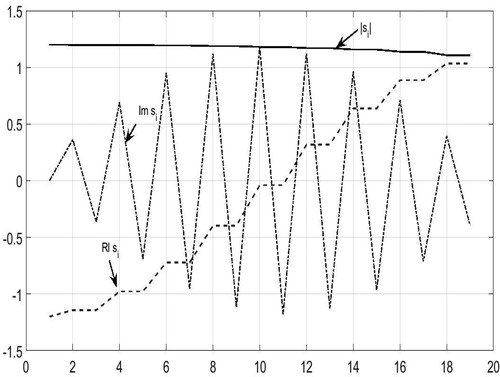${\mathbf{q}}_i$ are generally complex. Because A is real, eigenvalues, $s_j,$ are either pure real, or occur in complex conjugate pairs (see Fig. 17), with corresponding conjugate eigenvectors q. In the present case, the largest eigenvalue is pure real, with the rest being nine conjugate pairs. Magnitudes of the 25 eigenvalues are nearly constant and the inference is that the POP representation does little to economise the variability. The columns of eigenvectors are not orthogonal. The ${\alpha }_j(t)$ would normally be fit by least-squares to the observations through time, but because of the failure to produce a useful reduced data set, the subject is left here.

Fig. 17. Eigenvalues of the principal observation patterns (POPs), plotted as absolute value, real and imaginary parts.

References

- Abraham, J. P., Baringer, M., Bindoff, N. L., Boyer, T., Cheng, L. J. and co-authors. 2013. A review of global ocean temperature observations implications for ocean heat content estimates and climate change. Rev. Geophys. 51, 450–483. doi:10.1002/rog.20022
- Bengtsson, L., Hagemann, S. and Hodges, K. I. 2004. Can climate trends be calculated from reanalysis data? J. Geophys. Res. D11, D11111.
- Bindoff, N. L. and Mcdougall, T. J. 1994. McDougall diagnosing climate change and ocean ventilation using hydrographic data. J. Phys. Oceanogr. 24, 1137–1152. doi:10.1175/1520-0485(1994)024<1137:DCCAOV>2.0.CO;2
- Chan, D., Chan, D., Kent, E. C., Berry, D. I. and Huybers, P. 2019. Correcting datasets leads to more homogeneous early-twentieth-century sea surface warming. Nature 571, 393–397. doi:10.1038/s41586-019-1349-2
- Cronin, T. M. 2010. Paleoclimates: Understanding Climate Change Past and Present. Newyork: Columbia University Press, 441 pp.
- Fukumori, I., Heimbach, P., Ponte, R. M. and Wunsch, C. 2018. A dynamically-consistent ocean climatology and its temporal variations. Bull. Am. Met. Soc. 99, 2107–2127. doi:10.1175/BAMS-D-17-0213.1
- Fukumori, I., Wang, O., Fenty, I., Forget, G., Heimbach, P. and co-authors. 2017. ECCO Version 4 Release 3. Online at: ftp://ecco.jpl.nasa.gov/Version4/Release3/doc/v4r3_summary.pdf.
- Fukumori, I., Wang, O., Fenty, I., Forget, G., Heimbach, P. and co-authors. 2019. ECCO Version 4 Release 4. Online at: https://ecco.jpl.nasa.gov/drive/files/Version4/Release4/doc/v4r4_synopsis.pdf.
- Gebbie, G. and Huybers, P. 2019. The Little Ice Age and 20th-century deep Pacific cooling. Science 363, 70–74. doi:10.1126/science.aar8413
- Hasselmann K. 1988. PIPs and POPs: The reduction of complex dynamical systems using principal interactions and oscillation pattern. J. Geophys. Res. 93, 11015–11021. doi:10.1029/JD093iD09p11015
- Huang, R. X. 2010. Ocean Circulation: Wind-Driven and Thermohaline Processes. Cambridge University Press, Cambridge, xiii, 791 pp.
- Hughes, C. W. and Williams, S. D. P. 2010. The color of sea level: importance of spatial variations in spectral shape for assessing the significance of trends. J. Geophys. Res. Oceans. 115. DOI C1004810.1029/2010jc006102
- Jolliffe, I. T. 2002. Principal Component Analysis. 2nd ed. Springer-Verlag, New York, 487 pp.
- Jolliffe, I. T. and Cadima, J. 2016. Principal component analysis: a review and recent developments. Phil. Trans. Roy. Soc. A 374. DOI. 20150202 10.1098/rsta.2015.0202
- Klinger, B. A. and Haine, T. W. N. 2019. Ocean Circulation in Three Dimensions. Cambridge University Press, Cambridge, UK, 466 pp.
- LaCasce, J. H. 2017. The prevalence of oceanic surface modes. Geophys. Res. Lett. 44, 11097–110105.
- Lawson, C. L. and Hanson, R. J. 1995. Solving Least Squares Problems. SIAM, Philadelphia, 340 pp.
- Marshall, J., Adcroft, A., Hill, C., Perelman, L. and Heisey, C. 1997. A finite-volume, incompressible Navier Stokes model for studies of the ocean on parallel computers. J. Geophys. Res. 102, 5753–5766. doi:10.1029/96JC02775
- McWilliams, J. C. 2008. The nature and consequences of oceanic eddies. In: Ocean Modeling in an Eddying Regime (ed. M. W. Hecht and H. Hasumi). AGU Monograph, Am. Geophys. Un. Washington, pp. 5–15.
- Meyssignac, B., Boyer, T., Zhao, Z., Hakuba, M. Z., Landerer, F. W. and co-authors. 2019. Measuring global ocean heat content to estimate the Earth energy imbalance. Front. Mar. Sci. 6. DOI Unsp 43210.3389/fmars.2019.00432
- Pauthenet, E., Roquet, F., Madec, G., Sallee, J. B. and Nerini, D. 2019. The thermohaline modes of the global ocean. J. Phys. Oceangr. 49, 2535–2552. doi:10.1175/JPO-D-19-0120.1
- Pedlosky, J. 1996. Ocean Circulation Theory. Springer, Berlin, xi, 453 pp.
- Piecuch, C. G., Ponte, R. M., Little, C. M., Buckley, M. W. and Fukumori, I. 2017. Mechanisms underlying recent decadal changes in subpolar North Atlantic Ocean heat content. J. Geophys. Res. Oceans 122, 7181–7197. doi:10.1002/2017JC012845
- Sonnewald, M., Wunsch, C. and Heimbach, P. 2019. Unsupervised learning reveals geography of global ocean dynamical regions. Earth Space Sci. 6, 784–794. doi:10.1029/2018EA000519
- von Storch, H. and Zwiers, F. W. 2001. Statistical Analysis in Climate Research. Cambridge University Press, Cambridge, UK, 484 pp.
- Sverdrup, H. U., Johnson, M. W. and Fleming, R. H. 1942. The Oceans, Their Physics, Chemistry, and General Biology. Prentice-Hall, Inc., New York, 1087 pp.
- Vallis, G. K. 2017. Atmospheric and Oceanic Fluid Dynamics: Fundamentals and Large-Scale Circulation. Cambridge University Press, Cambridge UK, 946 pp.
- Wang, J., Flierl, G. R., LaCasce, J. H., McClean, J. L. and Mahadevan, A. 2013. Reconstructing the ocean’s interior from surface data. J. Phys. Oceanogr. 43, 1611–1626. doi:10.1175/JPO-D-12-0204.1
- Wills, R. C., Schneider, T., Wallace, J. M., Battisti, D. S. and Hartmann, D. L. 2018. Disentangling global warming, multidecadal variability, and El Niño in Pacific temperatures. Geophys. Res. Lett. 45, 2487–2496. doi:10.1002/2017GL076327
- Wortham, C. and Wunsch, C. 2014. A multi-dimensional spectral description of ocean variability. J. Phys. Oceanogr. 44, 944–966. doi:10.1175/JPO-D-13-0113.1
- Wunsch, C. 2006. Discrete Inverse and State Estimation Problems: With Geophysical Fluid Applications. Cambridge University Press, Cambridge, xi, 371 pp.
- Wunsch, C. 2015. Modern Observational Physical Oceanography. Princeton University Press, Princeton, 493 pp.
- Wunsch, C. 2016. Global ocean integrals and means, with trend implications. Annu. Rev. Mar. Sci. 8, 1–33. doi:10.1146/annurev-marine-122414-034040
- Wunsch, C. 2018. Towards determining uncertainties in global oceanic mean values of heat, salt, and surface elevation heat, salt, and surface elevation. Tellus 70, 1–14. doi:10.1080/16000870.2018.1471911
- Xu, Y. S. and Fu, L. L. 2012. The effects of altimeter instrument noise on the estimation of the wavenumber spectrum of sea surface height. J. Phys. Oceanogr. 42, 2229–2233. doi:10.1175/JPO-D-12-0106.1
- Zanna, L., Khatiwala, S., Gregory, J. M., Ison, J. and Heimbach, P. 2019. Global reconstruction of historical ocean heat storage and transport. Proc. Natl. Acad. Sci. USA. 116, 1126–1131. doi:10.1073/pnas.1808838115