Dynamically weighted hybrid gain data assimilation: perfect model testing

Abstract

Hybrid systems have become the state of the art among data assimilation methods. These systems combine the benefits of two other systems that are traditionally used in operational weather forecasting: an ensemble-based system and a variational system. One of the most recently proposed hybrid approaches is called hybrid gain (HG). It obtains the final analysis as a linear combination of two analyses, assuming that the innovations (i.e. the forecast and the set of observations used) between the two data assimilation methods are identical. A perfect model experiment was performed using the HG in the SPEEDY model to show a new methodology to assign different weights to the two analyses, LETKF and 3D-Var in the generation of the final analysis. Our new approach uses, in the assignment of the weights, the ensemble spread, considered to be a measure of uncertainty in the LETKF. Thus, it is possible to use the estimation of the uncertainty of the analysis that the LETKF provides, to determine where the system should give more weight to the LETKF or the 3D-Var analysis. For this purpose, we define a geographically varying weighting factor alpha, which multiplies the 3D-Var analysis, as the normalised spread for each variable at each level. Then, (1-alpha), which decreases with increasing spread, becomes the factor that multiplies the LETKF analysis. The underlying mechanism of the spread–error relationship is explained using a toy model experiment. The results are very encouraging: the original HG and the new weighted HG analyses have similar high quality and are better than both 3D-Var and LETKF. However, the dynamically weighted HG analyses are significantly more balanced than the original HG analyses are, which has probably contributed to the consistently improved performance observed in the weighted HG, which increases with time throughout the 5-day forecasts.

Keywords:

• data assimilation
• hybrid systems
• ensemble Kalman filter
• numerical weather prediction

1. Introduction

As the data assimilation (DA) systems become more complex because of the increase in observing datasets and model resolution, more effort has been focused on reducing the associated computational costs. Over the past 15 years, hybrid DA methodologies have become more popular, particularly for use in many operational weather forecast centres worldwide. Despite its general success, hybrid DA, from a practical (and mostly operational) perspective, can become computationally expensive. The main goal of hybrid DA is to combine two successful DA approaches: variational and ensemble-based. Hybrid DA was first proposed in 2000 (Hamill and Snyder 2000) to create a new covariance matrix based on the two other matrices: one from the EnKF (ensemble Kalman filter) and another from 3D-Var. After Hamill and Snyder (2000) demonstrated that the hybrid analysis was more accurate than either of the two original analyses, the same result was seen by other authors using different DA systems, as Etherton and Bishop (2004), who used the ETKF (ensemble transform Kalman filter) and 3D-Var to implement the hybrid DA system. In 2007, Wang et al. proposed a hybrid DA system through the combination of the ETKF and optimal interpolation. Zhang et al. (2009) perform what they called E4D-Var by the combination of the covariance matrix from EnKF and 4D-Var. All of these works, with their own details, found that the hybrid approach presents better results than the variational DA system or the ensemble DA system alone. Penny (2014) proposed a different approach for the hybrid system, aiming to reduce the computational load during the composition of the final analysis, and also reducing the human load by allowing the hybridisation to be applied to output files rather than modifying existing software systems. He called this algorithm hybrid/mean-LETKF, which belongs to a new class of hybrid DA methods: the hybrid gain (HG). From now, we will call the system as HG.

The HG aims to improve an ensemble-based system through the stability of the variational approach and to resolve rank deficiency in the ensemble forecast error covariance matrix that arises when the ensemble size is insufficient to resolve the growing error modes. Penny (2014) noted that traditional hybrids begin with a variational approach and incorporate the ensemble information through the ensemble-derived covariance matrix. Penny (2014) proposed instead an approach that begins with an EnKF and uses a variational approach to apply a correction in the model space to stabilise the EnKF. The specific algorithm proposed by Penny (2014) combines two analyses: one from the ensemble-based system and the other from the variational approach, which uses the ensemble analysis mean as the background. Thus, the final analysis is the result of this linear combination between two analyses, where the weight (alpha) given to the 3D-Var is a number between 0 and 1. The results suggest that alpha should be determined empirically, and that the optimal value depends on the number of ensemble members, observation coverage and localisation radius. In his study, Penny (2014) used the LETKF (local ensemble transform Kalman filter) and 3D-Var to implement the new HG with the Lorenz-96 model (Lorenz 1996).

The approach of Penny (2014) was tested with an operational model by Bonavita et al. (2015). The authors used the ECMWF (European Centre for Medium-Range Weather Forecasts) operational model combining the LETKF and the 4D-Var. They notice that that system was clearly more accurate than either 4D-Var or LETKF, and comparable to the operational ensemble data assimilation system (EDAS), also a hybrid system. According to the authors, the HG should be functionally equivalent to the hybrid B matrix, and they demonstrated some significant advantages of this method, such as its easy implementation. For the ocean, good results were also obtained by Penny et al. (2015), combining the LETKF with the NOAA’s operational global ocean data assimilation system (GODAS) (a 3D-Var analysis). The hybrid-GODAS was implemented at NCEP and reduced the root mean squared error (RMSE) and biases in the salinity and temperature compared to the 3D-Var and the LETKF. Most recently, Wespetal (2019) also used the HG and implemented this DA system in the SPEEDY model. Wespetal (2019) focused on finding better statistics for the construction of the climatological error covariance matrix in 3D-Var. Penny (2017) described how DA can be interpreted as a type of synchronisation problem. Wespetal (2019) compared the ‘NMC’ method to a method that used the perturbations of an ensemble forecast around the ensemble mean as a proxy of the model forecast error. In the same year, Houtekamer et al. (2019) implemented this approach in the Canadian Meteorological Centre (CMC). The authors modified the HG algorithm to leave half of the members unchanged and to recentre the other half on the EnVar analysis. Despite their differences, all these previous studies have something in common: in addition to using the HG, they used a fixed parameter as the alpha value. These studies tested some alpha values: $\alpha =0.0,\alpha =0.2,\alpha =0.5$ and α = 1.0. When the HG uses α = 0.5, it performs the final analysis using a half of LETKF and the other half of 3D-Var. On the other hand, when it uses $\alpha =0.2,$ it is using 80% from LETKF analysis mean and 20% from the 3D-Var. Most of the authors compare their results with the LETKF and 3D-Var, so, when α = 1.0 reflects the 3D-Var and $\alpha =0.0$ reflects the pure LETKF. Most recently, Chang et al. (2020) modified the HG algorithm to limit the variational correction to the subspace orthogonal to the ensemble perturbation subspace without the use of a hybrid weighting parameter, as the optimisation of such a parameter is non-trivial.

It is known that the errors in the LETKF are different from those in 3D-Var. Moreover, they present different spatial and temporal variabilities. The degree of uncertainty in an EnKF is related to its spread. However, this information has not yet been explored in the HG system, as proposed by Penny (2014). The goal of this work is to test the hypothesis that in any given DA cycle, LETKF and 3D-Var perform differently in different regions and that assigning a weight to each DA scheme based on the ensemble spread (as a proxy of the LETKF uncertainty) may benefit the hybrid system. We incorporate the ensemble spread information into the linear combination through a dynamic fit coefficient, weighing more the LETKF when it presents a small spread and the opposite when it presents a large spread. To support this proposed approach, we first performed a set of experiments using the Lorenz-96 as a toy model in a LETKF set up. The error–spread relationship is then assessed in order to demonstrate that there is a positive correlation between analysis and forecasts increase/decrease of ensemble spread and increase/decrease in analysis and forecast errors, respectively. A set of experiments to test the sensitivity of the alpha parameters are performed (including fixed values and the evolving dynamic value). Because this is a new methodology, a test is also performed to verify whether the geostrophic balance of the resulting analysis is within an acceptable range. Furthermore, the analysis of the HG using fixed optimal weights is compared to the proposed dynamic alpha for 5-day forecasts. This paper is structured as follows: Section 2 outlines the methods, including the details of the numerical model and DA system, the methodology by which the dynamic parameter is designed and the experimental setup; Section 3 presents the results and their discussion; and the conclusions are presented in Section 4.

2. Methodology

2.1. The model

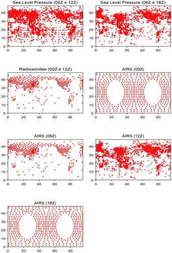
The atmospheric general circulation model used here is the SPEEDY model (Simplified Parameterisations, primitivE Equation DYnamics), developed by Molteni (2003). It has simplified sub-grid scale physics parameterisations that are computationally efficient. Although it is simplified, it retains the realistic basic characteristics of state-of-the-art models with more complex physics. The configuration of the SPEEDY model used here is the T30L7, which has seven vertical levels and a horizontal resolution of T30 that corresponds to approximately 200 km. This model solves the primitive equations for five prognostic variables: zonal wind (u), meridional wind (v), temperature (T), humidity (q) and sea level pressure (ps). Our perfect model experiment uses the SPEEDY model to perform the nature run. The nature run is also used as the ‘truth’ in the evaluation of the different experiments. The observations are extracted from the nature run, and random errors are added to them. Their spatial distribution is shown in Fig. 1. The observations are not evenly distributed across the globe, being compatible with the real distribution of these observations. The dots in the figure represent profiles of observations at each model level, not just single observation. They have surface pressure data, temperature, humidity and wind profiles. The radiosonde observations are only from 00Z and 12Z. The AIRS observations simulate AIRS satellite profiles of temperature and humidity for each time (00Z, 06Z, 12Z and 18Z).

Fig. 1. Spatial distribution of synthetic observations.

2.2. The data assimilation system

The HG algorithm used here is the hybrid/mean-LETKF proposed by Penny (2014) and implemented by Wespetal (2019) in the SPEEDY model, which under certain conditions is equivalent to forming the combination of gain matrices. This system solves Equation (1)(1) $${\mathbf{x}}_{HG}^a=(1-\alpha ){\overline{\mathbf{x}}}_{\mathit{LETKF}}^a+\alpha {\mathbf{x}}_{3D-\mathit{Var}}^a$$(1) , where ${\mathbf{x}}^{\mathbf{a}}{}_{HG}$ is the HG final analysis, ${\overline{\mathbf{x}}}_{\mathit{LETKF}}^a$ is the analysis mean from the LETKF, ${\mathbf{x}}_{3D-\mathit{Var}}^a$ is the analysis from the 3D-Var, which uses the ensemble analysis mean as the background, α is the coefficient that determines the weight that each system will have in the final analysis ($0\le \alpha \le 1$) and is a scalar. Then, the final HG analysis is (1) $${\mathbf{x}}_{HG}^a=(1-\alpha ){\overline{\mathbf{x}}}_{\mathit{LETKF}}^a+\alpha {\mathbf{x}}_{3D-\mathit{Var}}^a$$(1)

For the variational approach, we use the 3D-Var from Barker et al. (2004), with a tuned background error climatology for SPEEDY computed from forecast ensemble perturbations, as described in Descombes et al. (2015). A time-series of 6-h forecast ensembles for training the climatology was obtained for SPEEDY from independent LETKF assimilations of the synthetic observations, and the climatology variance for each assimilated model variable was tuned to best match the SPEEDY nature run. This system aims to solve the cost function in Equation (2)(2) $$\mathbf{J}({\mathbf{x}}^a)={({\mathbf{x}}^a-{\overline{\mathbf{x}}}^a)}^T{\mathbf{B}}^{-1}({\mathbf{x}}^a-{\overline{\mathbf{x}}}^a)+{(\mathbf{y}-\mathbf{H}({\mathbf{x}}^a))}^T{\mathbf{R}}^{-1}(\mathbf{y}-\mathbf{H}({\mathbf{x}}^a))$$(2) . (2) $$\mathbf{J}({\mathbf{x}}^a)={({\mathbf{x}}^a-{\overline{\mathbf{x}}}^a)}^T{\mathbf{B}}^{-1}({\mathbf{x}}^a-{\overline{\mathbf{x}}}^a)+{(\mathbf{y}-\mathbf{H}({\mathbf{x}}^a))}^T{\mathbf{R}}^{-1}(\mathbf{y}-\mathbf{H}({\mathbf{x}}^a))$$(2) where B is the background error covariance, R is the observation error covariance, ${\mathbf{x}}^a$ is the analysis state that minimises the cost function, ${\overline{\mathbf{x}}}^a$ is the state estimate determined from the ensemble, and y is the observation vector. The ensemble approach is the LETKF developed by Hunt et al. (2007), and it has been used with 16 members (K = 16). The LETKF analysis is calculated according to the following equations. ${\tilde{\mathbf{P}}}^a$ is the analysis error covariance in the ensemble space, and ${\mathbf{W}}^a$ is the weight for the analysis ensemble that we transform from the ensemble space back to the model space in Equation (5)(5) $${\mathbf{X}}^a={\mathbf{X}}^b{\mathbf{W}}^a$$(5) ; then, the analysis mean is computed as ${\overline{\mathbf{x}}}^a.$ (3) $${\tilde{\mathbf{P}}}^a={[\frac{(K-1)}{\rho }\mathbf{I}+{({\mathbf{Y}}^b)}^T{\mathbf{R}}^{-1}({\mathbf{Y}}^b)]}^{-1}$$(3) (4) $${\mathbf{W}}^a={[(K-1){\tilde{\mathbf{P}}}^a]}^{1/2}$$(4) (5) $${\mathbf{X}}^a={\mathbf{X}}^b{\mathbf{W}}^a$$(5) (6) $${\overline{\mathbf{w}}}^a={\tilde{\mathbf{P}}}^a{({\mathbf{Y}}^b)}^T{\mathbf{R}}^{-1}({\mathbf{y}}^o-{\overline{\mathbf{y}}}^b)$$(6) (7) $${\overline{\mathbf{x}}}^a={\mathbf{X}}^b{\overline{\mathbf{w}}}^a+{\overline{\mathbf{x}}}^b$$(7)

2.3. Spread–error relationship

In order to demonstrate the underlying hypothesis that the quality of the analysis and resulting forecasts are directly proportional to the respective ensemble spread, we employ a test model namely Lorenz-96 model (Lorenz 1996) which is a very useful tool to test hypotheses. One of the advantages is that it is a simple model which we can be executed multiple times, for many experiments with relatively minimum computational cost. Penny (2014) used this model to test the Hybrid/Mean-LETKF methodology, as well as Ying and Zhang (2015) used the Lorenz-96 model and the EnSRF to demonstrate that the adaptive covariance relaxation method can to improve filter performance with the presence of sampling errors over a range of severity. Chen and Kalnay (2019) used the ETKF in the Lorenz-96 model, in order to test the various configurations for the proactive quality control.

The numerical codes for the experiments performed in this study were obtained from the RIKEN International School on Data Assimilation, on Kobe Japan, during 2018 (http://www.data-assimilation.riken.jp/risda2018). The Lorenz-96 is described by the following equation (8) $$\frac{d{X}_i}{dt}=\left(X_{i+1}-X_{i-2}\right)X_{i+1}-X_i+F,X_{i\pm +1}=X_i$$(8) that simulates the advection, damping and forcing of a weather variable over a latitude circle where F represents a constant forcing. In this model, the first term represents ‘advection’ constructed to conserve kinetic energy, the second is damping, and the third is forcing. The boundaries are cyclic.

A perfect model experiment is conducted as follows: firstly a ‘truth’ or ‘nature’ run (i.e. the true evolution of the system) is performed using the Lorenz-96 model with n = 40 grids, from where a set of observations is selected randomly. Secondly, we assimilate the observations using a 30 members LETKF starting from an arbitrary state of the system and finally, the set of initial conditions produced in the previous step are used to run the ensemble forecasts.

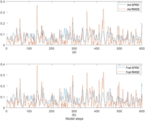
Figure 2 shows the temporal series of the RMSE and ensemble spread (SPRD) of the analysis (top panel) and forecasts (bottom panel) after spin-up time of approximately 50 time cycles.

Fig. 2. Time-series (assimilation cycles) of root mean square error (RMSE), in red, and ensemble spread (SPRD), in blue, of Lorenz-96 analysis (top panel) and forecasts (bottom panel).

In order to determine whether the hypothesis that the larger the ensemble spread the higher the resulting errors in the analysis and therefore lower confidence in the EnKF performance, the following steps were taken:

1. the first 200 steps were removed to account for mode spin-up;

2. the remaining 600 RMSE values of analysis/forecasts were rearranged in ascending order;

3. a new series of SPRD of analysis/forecasts values was created, indexed based on the corresponding RMSE values.

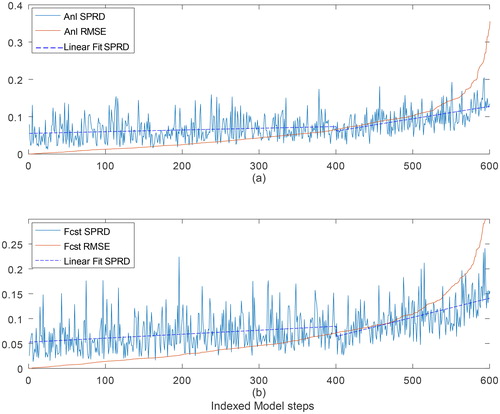
Hence, for each of the 40 points from the Lorenz-96 DA experiments, pairs of RMSE/SPRD were created, indexed by the increasing ordering of the SPRD values for both analysis and forecasts. Figure 3 shows the reordered values of SPRD and RMSE from a single point from the DA experiments. There is a small ascend in the RMSE before around 400 points followed by a steep ascend afterwards. The SPRD curve follows the growth of RMSE but at a lower rate with a positive correlation coefficient of around 0.53 for both analysis and forecasts. Two separate linear fit lines (blue dashes) were included to better illustrate the small and steep parts in the curve growth. The same procedure was applied to all 40 points with very similar behaviour of the spread–error relationship, resulting in an averaged 0.51 correlation coefficient. The positive correlation coefficients for both analysis and forecasts implied that both the analysis and the forecasts are worse when the spread is larger. So, the more accurate, the more confidence in the LETKF. The less accurate, the larger the spread, which makes the LETKF less reliable, and the 3D-Var more robust. Similar logic as also being stated in previous studies such as Houtekamer and Zhang (2016).

Fig. 3. Lorenz-96 LETKF analysis spread (SPRD) indexed by analysis error (RMSE) sorted from low to high values. Linear regression lines (dashed lines) show the small and steep growth rate of analysis spread as a function of analysis error growth (top panel). The spread–error relationship in the forecasts (bottom panel) shows similar results compared to the analysis error–spread relationship.

2.4. Dynamic alpha

The main purpose of a hybrid system is to combine two different systems, typically a variational system and an ensemble-based system. Thus, the dynamic fit coefficient (dynamic alpha) proposed here aims to use the extra information from the LETKF to assign different weights to each system in the HG linear combination. The LETKF spread was selected because it contains information associated with the degree of uncertainty in the mean state estimate. The proposal here is to better utilise spatially and temporally dependent information provided by LETKF via the ensemble spread. Thus, this work proposes replacing the fixed alpha (a scalar) from Equation (1)(1) $${\mathbf{x}}_{HG}^a=(1-\alpha ){\overline{\mathbf{x}}}_{\mathit{LETKF}}^a+\alpha {\mathbf{x}}_{3D-\mathit{Var}}^a$$(1) with a dynamic alpha (an evolving three-dimensional field), which is adjusted at each analysis step. This adjustment results in horizontally and vertically distributed weighting coefficient for each state variable, at each analysis time, instead of a single constant value for all variables in time and space. The dynamic alpha is obtained by normalising the ensemble spread fields from each variable (u, v, T, q and ps), at each model level (i.e. alpha values ranging from 0 to 1) and applying those normalised fields in Equation (1)(1) $${\mathbf{x}}_{HG}^a=(1-\alpha ){\overline{\mathbf{x}}}_{\mathit{LETKF}}^a+\alpha {\mathbf{x}}_{3D-\mathit{Var}}^a$$(1) . To obtain the alpha parameter we first calculate the standard deviation ${\sigma }_{x_{\mathit{ijl}}}$ of the ensemble members element-by-element (Equation 9(9) $${\sigma }_{x_{\mathit{ijl}}}=\sqrt{\frac{1}{K}\sum _{k=1}^K{[{(X_{\mathit{ijl}}^a)}_k-({\overline{x}}_{\mathit{ijl}}^a)]}^2}$$(9) ). Next, the minimum and maximum values of the standard deviation are calculated over all i, j grid points. Then the alpha parameter is computed by normalising ${\sigma }_{x_{\mathit{ijl}}}$ at each grid point i, j and level l (Equation 10(10) $${\alpha }_{x_{\mathit{ijl}}}=\frac{{\sigma }_{x_{\mathit{ijl}}}-\mathit{min}{({\sigma }_{x_{ij}})}_l}{\mathit{max}{({\sigma }_{x_{ij}})}_l-\mathit{min}{({\sigma }_{x_{ij}})}_l}$$(10) ). (9) $${\sigma }_{x_{\mathit{ijl}}}=\sqrt{\frac{1}{K}\sum _{k=1}^K{[{(X_{\mathit{ijl}}^a)}_k-({\overline{x}}_{\mathit{ijl}}^a)]}^2}$$(9) (10) $${\alpha }_{x_{\mathit{ijl}}}=\frac{{\sigma }_{x_{\mathit{ijl}}}-\mathit{min}{({\sigma }_{x_{ij}})}_l}{\mathit{max}{({\sigma }_{x_{ij}})}_l-\mathit{min}{({\sigma }_{x_{ij}})}_l}$$(10)

Unlike the weight in the traditional hybrid approach expressed as a constant scalar, the proposed dynamic alpha weight becomes now a time-varying three-dimensional tensor as shown in Equations (9)(9) $${\sigma }_{x_{\mathit{ijl}}}=\sqrt{\frac{1}{K}\sum _{k=1}^K{[{(X_{\mathit{ijl}}^a)}_k-({\overline{x}}_{\mathit{ijl}}^a)]}^2}$$(9) and (10)(10) $${\alpha }_{x_{\mathit{ijl}}}=\frac{{\sigma }_{x_{\mathit{ijl}}}-\mathit{min}{({\sigma }_{x_{ij}})}_l}{\mathit{max}{({\sigma }_{x_{ij}})}_l-\mathit{min}{({\sigma }_{x_{ij}})}_l}$$(10) .

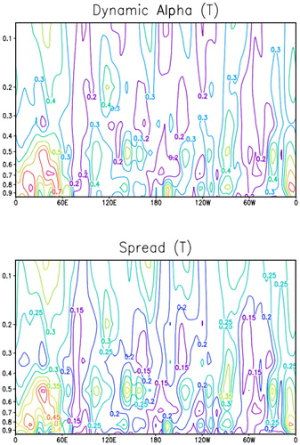
Figure 4 shows the dynamic alpha field (top) and the ensemble spread field (bottom) for the sea level pressure (ps), which was normalised to become the dynamic alpha, for the last day of the experiments (February 28, at 18Z). This figure shows an example of how the dynamic alpha works for one analyses step and for one model variable. This process is performed for the five model variables (u, v, T, q and ps) using their own spread, across the seven levels, which is exemplified in Fig. 5. In Fig. 5, we can see the vertical structure of the dynamic alpha (top) and ensemble spread (bottom), similar to the last figure, but for temperature (T). The cross-section was obtained at 45°S latitude. This latitude was chosen because we have the highest values of spread there and, consequently, the largest alpha values. The dynamic alpha follows the same pattern as the ensemble spread. When the spread is large more of the information from the 3D-Var is used, whereas when the spread is small more information from the LETKF is used.

Fig. 4. Horizontal structure of the dynamic alpha (top) and spread (bottom) of the sea level pressure (ps) on February 28 at 18Z.

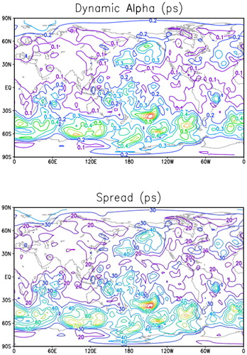
Fig. 5. Vertical structure of the dynamic alpha (top) and spread (bottom) of temperature (T) at the latitude 45°S on February 28 at 18Z.

According to Houtekamer and Zhang (2016), when a small ensemble size is used and it has the largest spread, the analysis quality will be low. Thus, the dynamic alpha is smaller the spread. If the spread is small, the dynamic alpha favours the LETKF analysis rather than the 3D-Var solution, which is less accurate.

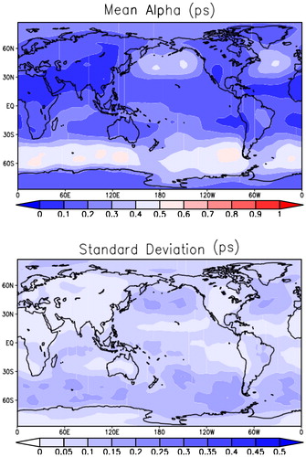
In Fig. 6, we have an example of the mean (top) and standard deviation (bottom) of the alpha throughout the period of this study for the sea level pressure. The mean shows the regions that use more LETKF or more 3D-Var. A bluer colour indicates that more LETKF was used in the analysis (alpha is close to zero), and a redder colour indicates more 3D-Var was used (alpha is close to one). In the regions where we have frequent transient systems, a large spread is common, and the HG with the alpha parameter gives more weight to 3D-Var. Comparing Fig. 1 and Fig. 6, it is clear that regions with a lack of observations, such as the oceans and the Southern Hemisphere, have a larger uncertainty than regions with better observational coverage. The standard deviation (bottom) shows how the alpha changed over these 3 months. This variation is very small; in this example, the maximum change in alpha compared to the mean was approximately 0.2.

Fig. 6. Mean (top) and standard deviation (bottom) of alpha of the sea level pressure for the entire period of this study (December, January and February).

2.5. Experimental setup

The experiments were performed during the boreal winter, simulated from 1 November 1982 to the end of February 1983. It should be noted that these are model simulated years and do not correspond to real years. To reduce the spin-up problems, only the trimester of December, January and February was evaluated. Eight experiments were performed using the SPEEDY model. First, five experiments using fixed alpha were run to estimate the best performing value of alpha. The tested alpha values were 0.1, 0.3, 0.5, 0.7 and 0.9. Then, two additional experiments using only the LETKF and only 3D-Var were performed for comparison. Finally, an experiment using the dynamic alpha (DYN) was performed. We evaluated the analyses and forecasts (120 h) computing their RMSE against the nature run, taken as truth.

3. Results

3.1. Assessment of 3D-Var and LETKF performances

In this section, we evaluate the performance of LETKF and 3D-Var separately. Table 1 shows the RMSE values of these two experiments for seven levels and four variables: pressure, temperature and wind components (u and v) over the globe. Table 1 shows the performance of both systems in the analysis. One can see that the LETKF is always better than 3D-Var, having the smallest errors at all levels and for all variables. These results are repeated when the regions are separated as hemispheres (we defined the Southern Hemisphere as the area between 80°S and 20°S and the Northern Hemisphere as the area between 20°N and 80°N) and tropics (defined as the area between 20°S and 20°N) (tables not shown). These results corroborate the results of Yang et al. (2009), who compared the LETKF and 3D-Var in a perfect model experiment. We believe that LETKF performs better than 3D-Var because of the combination of two effects: flow-dependent perturbation structures related to the errors of the day and ensemble averaging.

Table 1. Mean RMSE of pressure (ps), temperature (T) and wind components (u and v) over the globe in seven levels of the model.

	ps		T		u		v
	EKF	VAR	EKF	VAR	EKF	VAR	EKF	VAR
1	28.5	45.8	0.13	0.20	0.40	0.67	0.40	0.71
2			0.15	0.24	0.42	0.73	0.40	0.74
3			0.17	0.28	0.46	0.80	0.44	0.82
4			0.23	0.36	0.61	1.08	0.60	1.13
5			0.24	0.38	0.80	1.46	0.83	1.54
6			0.26	0.42	0.81	1.66	0.83	1.66
7			0.27	0.47	0.36	0.78	0.36	0.83

3.2. Analyses

This section aims to approximate the best case performance for a fixed value of alpha and compare it with the dynamic alpha. Thus, five experiments were performed with fixed alphas of 0.1, 0.3, 0.5, 0.7 and 0.9. The mean RMSE of the analysis for the vertical temperature profile, vertical humidity profile over the globe (on the top), and vertical u and v wind component profiles over the tropics (on the bottom) are shown in Fig. 7.

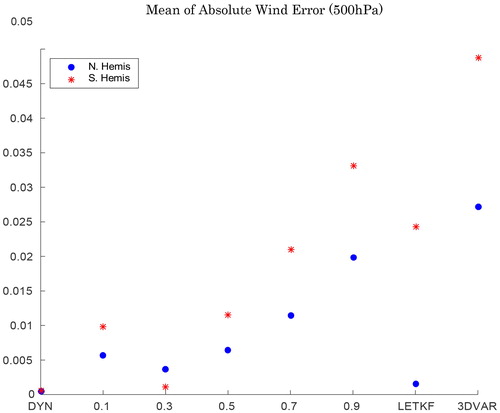
Fig. 7. Mean absolute wind error (500 hPa) in m/s for the eight experiments: dynamic alpha, $\alpha =0.1,\alpha =0.3,\alpha =0.5,\alpha =0.7,\alpha =0.9,$ LETKF and 3D-Var for the (red) Southern Hemisphere and (blue) Northern Hemisphere.

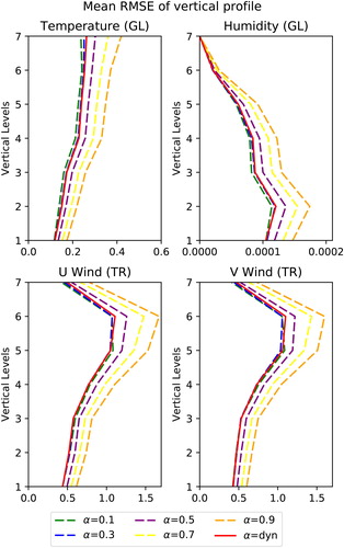
One can clearly see that α = 0.1 often showed the best results, whereas $\alpha =0.9$ showed the worst. Based on this result, when we use the HG, the error increases the more 3D-Var is used, and the error decreases the more LETKF is used. However, compared with the experiment using only the LETKF, the combination with the 3D-Var led to improved results. α = 0.1 (green dashed line) and α = 0.3 (blue dashed line) yielded better results than LETKF alone. It is noticeable that these results generally agree with the experiments conducted by Penny (2014) for the Lorenz-96 system, where the sensitivity of the system to the number of observations and ensemble members was tested and the accuracy decreased as alpha values increased. It implies (also supported by Fig. 1) that the current study is using a regime with sufficient observation coverage as well as ensemble size. Since for the cases we tested, larger weighting towards LETKF produced improved results except for the case of using only LETKF (α = 0), we further tested cases with alpha neighbouring 0.1. Both cases (α = 0.05 and α = 0.15) produced larger errors, thus indicating that the optimal value of alpha is likely in the interval between α = 0.05 and α = 0.15.

3.3. Balance of the system

The DA process is known to introduce some imbalance into the numerical forecasts, and the success of the initial conditions depends on how well balanced the control variables are with respect to the applied dynamics and physics parameterisation. Greybush et al. (2011) used a series of metrics to assess the imbalance of their experiments in the SPEEDY model. Thus, this section shows the results following Greybush et al. (2011).

Figure 8 shows the mean absolute wind error at 500 hPa. The x-axis indicates the experiments: dynamic alpha (DYN), $\alpha =0.1,\alpha =0.3,\alpha =0.5,\alpha =0.7,\alpha =0.9,$ LETKF, and 3D-Var. The DYN has the lowest error for both hemispheres.

Fig. 8. Mean of ageostrophic wind (500 hPa) in m/s for the eight experiments: dynamic alpha, $\alpha =0.1,\alpha =0.3,\alpha =0.5,\alpha =0.7,\alpha =0.9,$ LETKF and 3D-Var for the (top) Northern Hemisphere and (bottom) Southern Hemisphere. The blue points are the experiment values, and the red lines indicate the values for the nature run.

Figure 9 is the mean ageostrophic wind at 500 hPa for the Northern Hemisphere (top) and Southern Hemisphere (bottom). The x-axis shows the same experiments as in Fig. 8. The y-axis shows the values of the ageostrophic wind in m/s. The red line is the value of the nature run, which was used as the ‘truth’ state. Because the ageostrophic wind is a residual wind, we expected values close to zero. According to Greybush et al. (2011), when the imbalance of the analyses is larger than that in the true state, the DA is introducing an imbalance into the system. Thus, when the dynamic alpha is used, less imbalance is introduced in both hemispheres.

Fig. 9. Mean of ageostrophic wind (500 hPa) in m/s for the eight experiments: dynamic alpha, $\alpha =0.1,\alpha =0.3,\alpha =0.5,\alpha =0.7,\alpha =0.9,$ LETKF and 3D-Var for the (top) Northern Hemisphere and (bottom) Southern Hemisphere. The blue points are the experiment values, and the red lines indicate the values for the nature run.

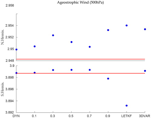
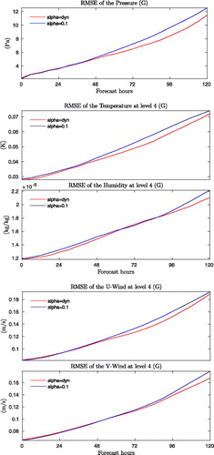
Fig. 10. RMSE of temperature, humidity, wind components (u and v) at level 4 and sea level pressure over the globe during the 120 h of forecast. The dynamic alpha experiment and experiment using α = 0.1 are shown as the red and blue lines, respectively.

3.4. Forecasts

Five-day forecasts were performed to compare the experiments using α = 0.1 and dynamic alpha. The results show that in most cases, the experiment using a dynamic alpha had better performance. Figure 10 shows the RMSE of the temperature, humidity, wind components (u and v) at level 4 (approximately 500 hPa) and sea level pressure over the globe during 120 h of forecast. These experiments were compared against the nature run. The dynamic alpha had better performance than even α = 0.1, as observed for most of the variables and levels.

The wind component does not follow a constant pattern. The dynamic alpha begins worse than α = 0.1 but this pattern changes during the forecast. This case occurs in the first and last levels of the model (not shown). In levels 2 and 3, the same occurred for the v component, as observed in level 5 for the u component. In level 6, the dynamic alpha is always better than α = 0.1.

For the sea level pressure, we can see that in the analyses the α = 0.1 is better. During the first forecast hours, both experiments had very close errors and, after 24 h, the dynamic alpha presented the smallest errors. These figures also suggest that the dynamic alpha has better skill beyond 5 days (for a perfect model).

4. Summary and conclusions

In this study, a three-dimensional parameter (‘alpha’ parameter) based on the LETKF ensemble spread was proposed as the weighting factor for the HG DA system (Penny 2014). The new suggested alpha was calculated based on the LETKF spread, in contrast to other hybrid methodologies that use a constant single value. Therefore, the dynamic alpha enables the combination of two hybrid components (LETKF and 3D-Var) to follow a spatial and vertical structure according to the uncertainties in the model ensemble, which is adjusted at each analysis step.

To test this new Weighting Factor HG methodology, the SPEEDY model was tested in LETKF and 3D-Var frameworks. The analyses and forecasts (up to 120 h) were evaluated for 3-month experiments (December, January and February), as was the effect that the dynamic alpha has on the system’s stability.

In order to support the computation of the HG based on the positive correlation between the analysis error and ensemble spread, we performed an experiment to assess the spread–error relationship in the LETKF using a simple toy model (Lorenz-96). The results showed that there is on average more than 0.5 correlation coefficient between analysis and forecast errors and respective ensemble spreads.

A set of experiments was conducted to find the optimal value of alpha to compare the results with the dynamic alpha. The optimal value was estimated to be in the interval between α = 0.05 and α = 0.15, in agreement with the experience that 3D-Var being less accurate than the LETKF. In the analyses (Fig. 7), we can see that for global temperature and for humidity, α = 0.1 shows the smallest error, whereas for the wind components in the tropics, the dynamic alpha was competitive with α = 0.1. However, comparing the results in the 120-h forecasts using these alpha values, we can see that using the α = 0.1 was worse. One of the hypotheses for the good results in the forecast is that the dynamic alpha has better-balanced analyses than do the constant alphas (as shown in Figs. 8 and 9). In other words, the use of the information obtained from the ensemble spread helps to reduce the imbalance between the EnKF and 3D-Var systems. The reason for the stability of the analyses using the dynamic alpha compared to that using the constant alpha is that we are essentially smoothing the analysis. This smoothing effect results in preventing large analysis increments from occurring next to much smaller increments. Such an end effect requires further investigation. Additionally, this study presents a methodology that permits to identify geospatially varying values of alpha that give near-optimal results without any necessary tuning.

In this particular study, the results show that the ensemble size of 16 is sufficient for the degrees of freedom in the present SPEEDY model configuration. Nevertheless, a proper sensitivity analysis based on testing different ensemble sizes to explore specific situations where the ensemble spread may not represent the system uncertainty is recommended for future studies.

The success of this perfect model experiment does not guarantee success with all atmospheric global models. Thus, we plan to test this hypothesis in more complex global models.

Acknowledgements

The authors thank Coordenação de Aperfeiçoamento de Pessoal de Nível Superior (CAPES) for the Sandwich scholarship and PhD scholarship. We also thank the Conselho Nacional de Desenvolvimento Científico e Tecnológico (CNPq) for the PhD scholarship.

Disclosure statement

No potential conflict of interest was reported by the authors.

References

- Barker, D. M., Huang, W., Guo, Y.-R., Bourgeois, A. J. and Xiao, Q. N. 2004. A three-dimensional variational data assimilation system for MM5: implementation and initial results. Mon. Wea. Rev. 132, 897–914. doi:10.1175/1520-0493(2004)132<0897:ATVDAS>2.0.CO;2
- Bonavita, M., Hamrud, M. and Isaksen, L. 2015. EnHF and hybrid gain ensemble data assimilation. Part II: EnKF and hybrid gain results. Mon. Wea. Rev. 143, 4865–4882. doi:10.1175/MWR-D-15-0071.1
- Chang, C.-C., Penny, S. G. and Yang, S.-C. 2020. Hybrid gain data assimilation using variational corrections in the subspace orthogonal to the ensemble. Mon. Wea. Rev. 148, 2331–2350. doi:10.1175/MWR-D-19-0128.1
- Chen, T.-C. and Kalnay, E. 2019. Proactive quality control: observing system simulation experiments with the Lorenz’96 model. Mon. Wea. Rev. 147, 53–67. doi:10.1175/MWR-D-18-0138.1
- Descombes, G., Auligné, T., Vandenberghe, F., Barker, D. M. and Barré, J. 2015. Generalized background error covariance matrix model (GEN_BE v2.0). Geosci. Model Dev. 8, 669–696. https://www.geosci-model-dev.net/8/669/2015/. doi:10.5194/gmd-8-669-2015
- Etherton, B. J. and Bishop, C. H. 2004. Resilience of hybrid ensemble/3DVAR analysis schemes to model error and ensemble covariance error. Mon. Wea. Rev. 132, 1065–1080. doi:10.1175/1520-0493(2004)132<1065:ROHDAS>2.0.CO;2
- Greybush, S. J., Kalnay, E., Miyoshi, T., Ide, K. and Hunt, B. R. 2011. Balance and ensemble Kalman filter localization techniques. Mon. Wea. Rev. 139, 511–522. doi:10.1175/2010MWR3328.1
- Hamill, T. M. and Snyder, C. 2000. A hybrid ensemble Kalman filter–3D variational analysis scheme. Mon. Wea. Rev. 128, 2905–2919. doi:10.1175/1520-0493(2000)128<2905:AHEKFV>2.0.CO;2
- Houtekamer, P. L., Buehner, M. and De La Chevrotière, M. 2019. Using the hybrid gain algorithm to sample data assimilation uncertainty. Q.J.R. Meteorol. Soc. 145, 35–56. https://rmets.onlinelibrary.wiley.com/doi/abs/10.1002/qj.3426. doi:10.1002/qj.3426
- Houtekamer, P. L. and Zhang, F. 2016. Review of the ensemble Kalman filter for atmospheric data assimilation. Mon. Wea. Rev. 144, 4489–4532. doi:10.1175/MWR-D-15-0440.1
- Hunt, B. R., Kostelich, E. J. and Szunyogh, I. 2007. Objective weather-map analysis. Phys. D Nonlinear Phenom. 230, 112–126. http://www.sciencedirect.com/science/article/B6TVK-4MNHXX0-3/2/43ec2cf5dffe5aacdf538cdeb90cd480. doi:10.1016/j.physd.2006.11.008
- Lorenz, E. 1996. Predictability – a problem partly solved. In: Proceedings of the ECMWF Seminar on Predictability, Vol. 1, Reading, UK, pp. 1–18. https://ci.nii.ac.jp/naid/10015392260/en/.
- Molteni, L. 2003. Atmospheric simulations using a GCM with simplified physical parametrizations. I: model climatology and variability in multi-decadal experiments. Climate Dyn. 20, 175–191. doi:10.1007/s00382-002-0268-2
- Penny, S. G. 2014. The hybrid local ensemble transform Kalman filter. Mon. Wea. Rev. 142, 2139–2149. doi:10.1175/MWR-D-13-00131.1
- Penny, S. G. 2017. Mathematical foundations of hybrid data assimilation from a synchronization perspective. Chaos 27, 126801. doi:10.1063/1.5001819
- Penny, S. G., Behringer, D. W., Carton, J. A. and Kalnay, E. 2015. A hybrid global ocean data assimilation system at NCEP. Mon. Wea. Rev. 143, 4660–4677. doi:10.1175/MWR-D-14-00376.1
- Wang, X., Hamill, T. M., Whitaker, J. S. and Bishop, C. H. 2007. A comparison of hybrid ensemble transform Kalman filter–optimum interpolation and ensemble square root filter analysis schemes. Mon. Wea. Rev. 135, 1055–1076. doi:10.1175/MWR3307.1
- Wespetal, M. E. 2019. Advanced data assimilation for a mars atmospheric reanalysis. Thesis Prospectus, University of Maryland, College Park, MD.
- Yang, S.-C., Corazza, M., Carrassi, A., Kalnay, E. and Miyoshi, T. 2009. Comparison of local ensemble transform Kalman filter, 3DVAR, and 4DVAR in a quasigeostrophic model. Mon. Wea. Rev. 137, 693–709. doi:10.1175/2008MWR2396.1
- Ying, Y. and Zhang, F. 2015. An adaptive covariance relaxation method for ensemble data assimilation. Q.J.R. Meteorol. Soc. 141, 2898–2906. https://rmets.onlinelibrary.wiley.com/doi/pdf/10.1002/qj.2576. doi:10.1002/qj.2576
- Zhang, F., Zhang, M. and Hansen, J. 2009. Coupling ensemble Kalman filter with four-dimensional variational data assimilation. Adv. Atmos. Sci. 26, 1–8. doi:10.1007/s00376-009-0001-8