An anisotropic formulation of the parametric Kalman filter assimilation

Abstract

In geophysics, the direct application of covariance matrix dynamics described by the Kalman filter (KF) is limited by the high dimension of such problems. The parametric Kalman filter (PKF) is a recent alternative to the ensemble Kalman filter, where the covariance matrices are approximated by a covariance model featured by a set of parameters. The covariance dynamics is then described by the time evolution of these parameters during the analysis and forecast cycles. This study focuses on covariance model parametrized by the variance and the local anisotropic tensor fields (VLATcov). The analysis step of the PKF for VLATcov in a 2D/3D domain is first introduced. Then, using 2D univariate numerical investigations, the PKF is shown to be able to provide a low numerical cost approximation of the Kalman filter analysis step, even for anisotropic error correlation functions. Moreover the PKF has been shown able to reproduce the KF over several assimilation cycles in a transport dynamics. An extension toward the multivariate situation is theoretically studied in a 1D domain.

Keywords:

• data assimilation
• parametric Kalman filter
• univariate analysis
• multivariate analysis

1. Introduction

In geophysical applications, the aim of data assimilation is to estimate the state of a system (e.g. ocean, atmosphere, concentration of a chemical species for air quality). Currently, the size of such a numerical representation can be extremely large, on the order of 10⁷–10⁹ degrees of freedom. However, due to the sensitivity to the initial conditions, the heterogeneity of the observational network and noise that affect the observations, the real state can only be estimated with uncertainty (Daley, 1991).

A major theoretical and numerical tool used in assimilation is the Kalman filter (Kalman, 1960), which relies on assumptions of Gaussianity for the uncertainty and of linearity for the dynamics (and the observational operators). Therefore, due to its Gaussianity, any probability distribution is then entirely determined by the knowledge of its mean state and its error covariance matrix. The linearity assumption preserves the Gaussianity of the uncertainty during the time evolution from the dynamics and the update from the analysis step. The Kalman filter describes the time evolution of the mean state and the error covariance matrix during the analysis and forecast steps. Despite the theoretical framework offered by the Kalman filter, practical implementations are limited by the huge sizes of the problems considered in geophysics, only a few applications exist of the standard purely linear Kalman filter, with explicit temporal evolution of the complete covariance matrix of forecast error e.g. in air quality (Ménard et al., 2000; Ménard and Chang, 2000). For example, the size of the covariance matrices can reach a number of degrees of freedom on the order of 10¹⁴–10¹⁸, far beyond the current capacities of supercomputers.

To bypass these limitations, ensemble methods have been introduced to approximate the state error covariance matrices using ensemble estimations such as the ensemble Kalman filter (EnKF) (Evensen, 2009). In this way, it is possible to account for the nonlinear behaviour of the dynamics and to handle the huge error covariance matrices during the analysis and forecast steps. Operational implementations of the EnKF have shown the ability of this algorithm to be applied in geophysics (Houtekamer et al., 2005; Coman et al., 2012; Sakov and Sandery, 2015). The EnKF is a robust algorithm that has been applied to a wide range of systems, from theoretical systems, e.g. the classic Lorenz-95 system (Bocquet et al., 2015), to operational systems in the ocean or atmosphere. Because it is problem-independent, EnKF is easy to apply to a multitude of different situations. However, the EnKF also suffers from some drawbacks. In fact, the independence from the problem is also a limitation: the EnKF does not take advantage of possible simplifications related to type of dynamics governing a system. For instance, for a transport dynamics (advection of a scalar field by the wind), the forecast error variance field evolves by the same transport equation, that is simple to compute e.g. the variance field is predicted by using the same numerical scheme as the one used for solving the transport dynamics of the scalar field (Cohn, 1993; Pannekoucke et al., 2016, 2020). When using an EnKF, the variance field for the transport equation is performed as follows: the initial uncertainty is pushed forward by forecasting each member of the ensemble, then the variance is estimated. This routine to compute the variance is the same for any dynamics e.g. a Lorenz63 or the weather (Evensen, 2009). Hence, the EnKF does not take advantage of the partial differential equations that govern the dynamics of geophysical flows or the transport of the mixing ratio in atmospheric chemistry. While the EnKF is naturally parallelized, ensemble predictions are often performed at a lower resolution than the operational forecast to balance the computational burden from running the multiple model runs required for an ensemble. Since only a dozen members are generally considered, the small ensemble size leads to large distant correlations due to the sampling noise and implies the need to consider localization strategies.

In a recent study, another route to approximating the Kalman filter (KF) error covariance dynamics was proposed. This approach, called the parametric Kalman filter (PKF), consists of a parametric formulation where the forecast and the analysis error covariance matrices are approximated by a covariance model. For example, when choosing the covariance model based on the diffusion equation (Weaver and Courtier, 2001), the time evolution of the KF error covariance matrices can be approximated by the dynamics of the error variance and the error diffusion tensor field during the analysis and forecast steps (Pannekoucke et al., 2016, 2018b). An illustration using the 1D advection–diffusion of a passive tracer has shown the potential of this approach. In particular, this simple framework illustrates the complex interactions due to the physical diffusion process, which causes a coupling between the error variance and the error diffusion metric tensor to appear. This simple framework also demonstrates interactions due to stretching via advection. In its forecast step, the PKF relies on the equations that govern the dynamics and this problem dependency is both the strength and the weakness of the PKF. It is a weakness because the dynamics of the parameters has to be designed from the specific partial differential equations of the system; however, this is the price for not using an ensemble. The strength of the method is to dramatically reduce the numerical cost of calculating the covariance forecast. Note that a splitting method exists that can help build new parameter dynamics from already known dynamics. The splitting method has been used in nonlinear dynamics with the nonlinear advection–diffusion equation (or Burgers’ equation), which confirmed the potential of the PKF approach to solve the extended Kalman filter via a Gaussian second-order filter in the forecast step (Pannekoucke et al., 2018a). This extension to a nonlinear dynamics problem revealed challenges facing the design of the parameter dynamics by highlighting difficulties when handling some processes, for example, physical diffusion. However, it also illustrated the benefits of formulating the dynamics of the uncertainty resulting from the concurrence between the advection and the physical diffusion; for this simple system, the PKF reproduces the KF for the mid-term forecast in the tangential linear regime. If forecasting the uncertainty is a real challenge, it only represents one part of the KF, and being able to write equations for the parameter update during the analysis step is an astonishing result with interesting consequences. One of these consequences is that the PKF does not suffer from spurious long-range correlations when the modelled correlation functions are compactly numerically supported, which is the case for the correlations modelled from the diffusion equation.

Because the PKF has been primarily designed in 1D, it is essential to extend the PKF analysis step in 2D and 3D and to assess its ability to produce a correct update of the anisotropy of the forecast error statistics. The formulation of the PKF analysis update should be done only one time for each choice of covariance model: the equation for the analysis update is independent of the forecast dynamics. However, in its initial derivation, the PKF analysis only weakly represents the anisotropies because it relies on locally homogeneous Gaussian functions. In addition, the update of the forecast-error anisotropy tensor has only been settled in 1D with an extrapolation to higher dimensional cases. These two points appear to be the main drawbacks of the PKF analysis step and need to be addressed. As another point, if the PKF is able to describe the update of the forecast error statistics with an appropriate description of the anisotropy, then it should also be possible to estimate the analysis state.

To tackle these three points, the current contribution focuses on the analysis step, assessing the ability of the PKF formulation to approximate the KF analysis statistics, a prerequisite for real applications. To do so, we consider the family of covariance models parametrized by the variance field and the local anisotropic tensors (VLATcov); and introduce then evaluate the PKF for VLATcov.

This manuscript is organized as follows. Section 2 reviews some background on the KF and introduces the PKF. Then, Sec. 3 focuses on the PKF for VLATcov. The covariance model based on a diffusion equation is presented and a surrogate for this covariance model is introduced, both covariance model are VLATcov. Numerical investigations are then presented in Sec. 4, which first compares the PKF to the KF analysis step for a univariate assimilation in a 2D domain followed by a comparison over several assimilation cycles (analysis and forecast steps) for a transport equation. In order to better understand the limits of this work, Sec. 5 presents a simple multivariate experiment in a 1D domain. Conclusions are made in the final section, Sec. 6.

2. Background and new analytical results on Kalman filter

2.1. Analysis step in the Kalman filter

In operational forecasting, the true state ${\mathcal{X}}^t$ of a system (e.g. the ocean, the atmosphere or the mixing ratios of chemical species in atmospheric chemistry) is unknown. Data assimilation aims to compute the optimal estimation of ${\mathcal{X}}^t,$ that is, the analysis state ${\mathcal{X}}^a,$ by combining the observations ${\mathcal{Y}}^o$ and the forecast state ${\mathcal{X}}^f.$ The dimensions of ${\mathcal{X}}^t$ and ${\mathcal{Y}}^o$ are denoted by n and p, respectively. For linear dynamics and additive Gaussian errors uncorrelated in time, the formalism that describes the evolution of the uncertainty over time, and that relies on the Bayesianity, is given by the Kalman filter (KF) equations (Kalman, 1960). The analysis step updates the forecast uncertainty to account for the information from the observations following (1a) $${\mathcal{X}}^a={\mathcal{X}}^f+\mathbf{K}\left({\mathcal{Y}}^o-\mathbf{H}{\mathcal{X}}^f\right),$$(1a) (1b) $${\mathbf{P}}^a=({\mathbf{I}}_n-\mathbf{KH}){\mathbf{P}}^f,$$(1b) where $\mathbf{K}={\mathbf{P}}^f{\mathbf{H}}^{\mathrm{T}}{(\mathbf{H}{\mathbf{P}}^f{\mathbf{H}}^{\mathrm{T}}+\mathbf{R})}^{-1}$ is the gain matrix with the superscript T denoting the transpose operator; $\mathbf{H}$ is the (linear) observation operator that maps the model state into the observation space; ${\mathbf{P}}^f=\mathbb{E}({\mathit{\epsilon }}^f{\mathit{\epsilon }}^f{}^{\mathrm{T}})$ is the covariance matrix of the forecast error defined by ${\mathit{\epsilon }}^f={\mathcal{X}}^f-{\mathcal{X}}^t,$ where $\mathbb{E}$ denotes the expectation operator; ${\mathbf{P}}^a=\mathbb{E}({\mathit{\epsilon }}^a{\mathit{\epsilon }}^a{}^{\mathrm{T}})$ is the covariance matrix of the analysis error defined by ${\mathit{\epsilon }}^a={\mathcal{X}}^a-{\mathcal{X}}^t;$ $\mathbf{R}=\mathbb{E}({\mathit{\epsilon }}^o{\mathit{\epsilon }}^o{}^{\mathrm{T}})$ is the covariance matrix of the observation error defined by ${\mathit{\epsilon }}^o={\mathcal{Y}}^o-\mathbf{H}{\mathcal{X}}^t;$ and ${\mathbf{I}}_n$ is the identity matrix with dimension n. In above, the Gaussianity of the error means that the errors are modelled as Gaussian processes with zero mean i.e. $\mathbb{E}({\mathit{\epsilon }}^f)=0,$ $\mathbb{E}({\mathit{\epsilon }}^o)=0,$ and $\mathbb{E}({\mathit{\epsilon }}^a)=0.$ Note that the analysis step Eq. (1) coincides with the best linear unbiased estimator (BLUE): a sub-optimal estimator which only needs the existence of a covariance matrix for the unbiased error, and relaxes the Gaussian assumption (Daley, 1991).

While the KF equations are simple relations from linear algebra, their use is limited to problems with small sizes. Moreover, little analytical results are known about the KF equations that could be used in practice.

2.2. Analysis state and variance update for a single observation assimilation

In general, the matrix inversion in the analysis equation, Eq. (1a)(1a) $${\mathcal{X}}^a={\mathcal{X}}^f+\mathbf{K}\left({\mathcal{Y}}^o-\mathbf{H}{\mathcal{X}}^f\right),$$(1a) , makes it difficult to simplify this relation.

However, the assimilation of a single direct observation can leads to some analytical results. For an observation located at a grid point ${\mathit{x}}_l$ and of value ${\mathcal{Y}}^o({\mathit{x}}_l),$ when the observation operator is the linear projector $\mathbf{H}{\mathcal{X}}^f={\mathcal{X}}^f({\mathit{x}}_l),$ the analysis equation becomes (2) $$\begin{array}{c}{\mathcal{X}}^a(\mathit{x})={\mathcal{X}}^f(\mathit{x})+{\sigma }^f(\mathit{x}){\rho }_{{\mathit{x}}_l}^f(\mathit{x})\\ \frac{{\sigma }^f({\mathit{x}}_l)}{V^f({\mathit{x}}_l)+V^o({\mathit{x}}_l)}({\mathcal{Y}}^o({\mathit{x}}_l)-{\mathcal{X}}^f({\mathit{x}}_l)),\end{array}$$(2) where $V^o({\mathit{x}}_l)=\mathbb{E}\left[{\mathit{\epsilon }}^o{({\mathit{x}}_l)}^2\right]$ is the observational-error variance associated with the observation, $V^f=\mathbb{E}\left[{({\mathit{\epsilon }}^f)}^2\right]$ is the field of forecast-error variance and standard-deviation ${\sigma }^f=\sqrt{V^f},$ and ${\rho }_{{\mathit{x}}_l}^f(\mathit{x})$ is the forecast-error correlation function defined by ${\rho }^f({\mathit{x}}_l,\mathit{x})=\mathbb{E}\left[{\mathit{\epsilon }}^f({\mathit{x}}_l){\mathit{\epsilon }}^f(\mathit{x})\right]/(\sqrt{V^f({\mathit{x}}_l)}\sqrt{V^f(\mathit{x})}).$

Therefore, the forecast is modified around the observation location with a pattern characteristic of the forecast error correlation. This simplified expression, which does not apply to non-local observations, such as satellite radiance data, constitutes one of the classic results of optimal interpolation.

Because the forecast is locally updated, the variance field also changes in the vicinity of the observation position leading to the second classic result (Daley, 1991, pp. 146–147): (3) $$V^a(\mathit{x})=V^f(\mathit{x})\left(1-{[{\rho }_{{\mathit{x}}_l}^f(\mathit{x})]}^2\frac{V^f({\mathit{x}}_l)}{V^f({\mathit{x}}_l)+V^o({\mathit{x}}_l)}\right),$$(3) for which the origin is given in Appendix B for self-consistency.

Like for the variance field, the shape of the correlation functions is influenced by the assimilation of an observation as discussed now.

2.3. Update of the local shape of the error-correlation function for a single observation assimilation

This part details how to characterize the local shape of the error-correlation function and how it is modified by the assimilation of a single observation.

2.3.1. Definition and diagnosis of the local shape

When the forecast-error is a differential random field, the local shape of the correlation is characterized by the so-called local forecast-error metric tensor ${\mathit{g}}^f(\mathit{x}),$ (4) $$g_{ij}^f(\mathit{x})=-{\partial }_{x^i{x}^j}^2{\rho }^f{(\mathit{x},\mathit{y})}_{|\mathit{y}=\mathit{x}},$$(4) that appears in the Taylor expansion of the correlation function (Daley, 1991; Hristopulos, 2002; Pannekoucke et al., 2014), (5) $${\rho }^f(\mathit{x},\mathit{y})\approx 1-\frac{1}{2}\left|\right|\mathit{y}-\mathit{x}|{|}_{{\mathit{g}}^f(\mathit{x})}^2.$$(5)

In particular, ${\mathit{g}}^f(\mathit{x})$ is a symmetric positive-definite matrix that prevents the correlation value from being larger than one. The metric tensor is related to the statistics of the random field ${\mathit{\epsilon }}^f$ according to the formula (Belo Pereira and Berre, 2006) (6) $$g_{ij}^f(\mathit{x})=\mathbb{E}\left[{\partial }_{x^i}\left(\frac{{\mathbf{\epsilon }}^f}{{\sigma }^f}\right){\partial }_{x^j}\left(\frac{{\mathbf{\epsilon }}^f}{{\sigma }^f}\right)\right](\mathit{x}),$$(6) where ${\sigma }^f=\sqrt{V^f}$ denotes the forecast-error standard deviation.

The expression Eq. (6)(6) $$g_{ij}^f(\mathit{x})=\mathbb{E}\left[{\partial }_{x^i}\left(\frac{{\mathbf{\epsilon }}^f}{{\sigma }^f}\right){\partial }_{x^j}\left(\frac{{\mathbf{\epsilon }}^f}{{\sigma }^f}\right)\right](\mathit{x}),$$(6) of the metric tensor proves very useful during theoretical manipulations (a proof of Eq. (6)(6) $$g_{ij}^f(\mathit{x})=\mathbb{E}\left[{\partial }_{x^i}\left(\frac{{\mathbf{\epsilon }}^f}{{\sigma }^f}\right){\partial }_{x^j}\left(\frac{{\mathbf{\epsilon }}^f}{{\sigma }^f}\right)\right](\mathit{x}),$$(6) is provided in Appendix A). Eq. (6)(6) $$g_{ij}^f(\mathit{x})=\mathbb{E}\left[{\partial }_{x^i}\left(\frac{{\mathbf{\epsilon }}^f}{{\sigma }^f}\right){\partial }_{x^j}\left(\frac{{\mathbf{\epsilon }}^f}{{\sigma }^f}\right)\right](\mathit{x}),$$(6) ensures that the resulting metric tensor is symmetric, but also positive: for any vector $\delta \mathit{x},$ $\delta {\mathit{x}}^{\mathrm{T}}{\mathit{g}}^f(\mathit{x})\delta \mathit{x}=\mathbb{E}\left[{(\delta {\mathit{x}}^{\mathrm{T}}\nabla \left(\frac{{\mathit{\epsilon }}^f}{{\sigma }^f}\right))}^2\right]\ge 0;$ but the definiteness of ${\mathit{g}}^f$ results from the differentiability of ${\mathit{\epsilon }}^f$ (Hristopulos, 2002). In geoscience, where the flow is governed by PDEs with some physical (or turbulent) diffusion, the assumption of error differentiability makes sense.

In practice, the geometry of the local metric tensor is contravariant: the direction of largest correlation anisotropy corresponds to the principal axes of smallest eigenvalue for the metric tensor. Thus, it is useful to introduce the local aspect tensor (Purser et al., 2003) whose the geometry goes as the correlation, and defined as the inverse of the metric tensor (7) $${\mathit{s}}^f(\mathit{x})={\left({\mathit{g}}^f(\mathit{x})\right)}^{-1},$$(7) where the superscript ⁻¹ denotes the matrix inverse. The metric as well as the aspect tensor can be used to characterize correlation functions, according to the following definitions: when the aspect tensor is the same for each position, then the correlation functions are said to be homogeneous, and when the aspect tensor is proportional to the identity matrix, the correlation is isotropic; conversely, when the aspect tensor is different for each position, the correlation functions are heterogeneous, and when the aspect tensor is not proportional to the identity matrix, the correlation is anisotropic. These definitions result from the local aspect tensor field being considered as a diagnostic of the correlation functions; however, a more rigorous global definition of the homogeneity and the isotropy can be found in Gaspari and Cohn (1999).

To quantify the magnitude of the anisotropy, the local aspect tensor $\mathit{s}$ can be compared to its isotropic part defined as $${\mathit{s}}_{\text{iso}}=\frac{1}{d}\text{Tr}(\mathit{s}){\mathbf{I}}_d,$$ where $\text{Tr}(·)$ denotes the matrix trace operator and d denotes the spatial dimension. Therefore, the isotropy deviation can be defined as the distance (8) $${\delta }_{\text{iso}}=\frac{1}{d-1}\left|\right||\mathit{s}{({\mathit{s}}_{\text{iso}})}^{-1}-{\mathbf{I}}_d|\left|\right|,$$(8) where $\left|\right||·|\left|\right|$ is the multiplicative norm defined by $\left|\right|\left|\mathbf{U}\right|\left|\right|=\underset{\left|\right|\mathit{x}\left|\right|=1}{\text{max}}\left|\right|\mathbf{U}\mathit{x}\left|\right|$ for any matrix $\mathbf{U}.$ This isotropy deviation is a simple scalar diagnostic for which ${\delta }_{\text{iso}}\in [0,1].$ An isotropy deviation of ${\delta }_{\text{iso}}=0$ stands for an isotropic tensor, while a deviation of ${\delta }_{\text{iso}}=1,$ for d = 2, stands for a purely anisotropic tensor i.e. a singular tensor. In addition, the isotropic part generates an isotropic length scale defined as (9) $$L_{\text{iso}}={(\text{Tr}(\mathit{s})/d)}^{1/2},$$(9) which describes the spread of the local error correlation functions within a single scalar field. When the scale of variation of the aspect tensor is smaller than the isotropic length scale (Eq. (9)(9) $$L_{\text{iso}}={(\text{Tr}(\mathit{s})/d)}^{1/2},$$(9) ), the correlation is said to be locally homogeneous.

2.3.2. Update of the local metric tensor for a single observation

As far as we know, there is no classical formula for updating the metric tensor field, whereas it should change at the observation point, but also in its vicinity. After some calculations, which are given in Appendix B, the local metric tensors update as (10) $$\begin{array}{c}{\mathit{g}}^a(\mathit{x})=\frac{V^f(\mathit{x})}{V^a(\mathit{x})}{\mathit{g}}^f(\mathit{x})+\\ \frac{1}{4V^f(\mathit{x})V^a(\mathit{x})}\left[\nabla V^f{(\nabla V^f)}^{\mathrm{T}}\right](\mathit{x})-\\ \frac{1}{V^a(\mathit{x})}\frac{V^f({\mathit{x}}_l)}{V^f({\mathit{x}}_l)+V^o({\mathit{x}}_l)}\\ \left[\nabla ({\sigma }^f{\rho }_{{\mathbf{x}}_l}^f){\left(\nabla ({\sigma }^f{\rho }_{{\mathbf{x}}_l}^f\right)}^{\mathrm{T}}\right](\mathit{x})-\\ \frac{1}{4{(V^a(\mathit{x}))}^2}\left[\nabla V^a{(\nabla V^a)}^{\mathrm{T}}\right](\mathit{x}).\end{array}$$(10)

Note that, because the analysis metric tensor appears as the difference of symmetric positive tensors, there is no guarantee that the numerical computation will lead to a positive matrix. However, when the analysis and forecast error variance fields are locally homogeneous, i.e. when $\frac{1}{V^f}\nabla V^f$ and $\frac{1}{V^a}\nabla V^a$ can be neglected, the analysis error metric tensor field simplifies to (11) $${\mathit{g}}^a(\mathit{x})\approx \frac{V^f(\mathit{x})}{V^a(\mathit{x})}{\mathit{g}}^f(\mathit{x}),$$(11) which can be written, in terms of the local aspect tensor, as (12) $${\mathit{s}}^a(\mathit{x})\approx \frac{V^a(\mathit{x})}{V^f(\mathit{x})}{\mathit{s}}^f(\mathit{x}),$$(12) which is a surprisingly simple result that ensures the positiveness of the tensor in numerical computations (for all positions $\mathit{x},$ $0\le V^a(\mathit{x})\le V^f(\mathit{x})$).

2.4. Discussion on the KF

It is important to note that Eqs. (2)(2) $$\begin{array}{c}{\mathcal{X}}^a(\mathit{x})={\mathcal{X}}^f(\mathit{x})+{\sigma }^f(\mathit{x}){\rho }_{{\mathit{x}}_l}^f(\mathit{x})\\ \frac{{\sigma }^f({\mathit{x}}_l)}{V^f({\mathit{x}}_l)+V^o({\mathit{x}}_l)}({\mathcal{Y}}^o({\mathit{x}}_l)-{\mathcal{X}}^f({\mathit{x}}_l)),\end{array}$$(2) , (3)(3) $$V^a(\mathit{x})=V^f(\mathit{x})\left(1-{[{\rho }_{{\mathit{x}}_l}^f(\mathit{x})]}^2\frac{V^f({\mathit{x}}_l)}{V^f({\mathit{x}}_l)+V^o({\mathit{x}}_l)}\right),$$(3) and (10)(10) $$\begin{array}{c}{\mathit{g}}^a(\mathit{x})=\frac{V^f(\mathit{x})}{V^a(\mathit{x})}{\mathit{g}}^f(\mathit{x})+\\ \frac{1}{4V^f(\mathit{x})V^a(\mathit{x})}\left[\nabla V^f{(\nabla V^f)}^{\mathrm{T}}\right](\mathit{x})-\\ \frac{1}{V^a(\mathit{x})}\frac{V^f({\mathit{x}}_l)}{V^f({\mathit{x}}_l)+V^o({\mathit{x}}_l)}\\ \left[\nabla ({\sigma }^f{\rho }_{{\mathbf{x}}_l}^f){\left(\nabla ({\sigma }^f{\rho }_{{\mathbf{x}}_l}^f\right)}^{\mathrm{T}}\right](\mathit{x})-\\ \frac{1}{4{(V^a(\mathit{x}))}^2}\left[\nabla V^a{(\nabla V^a)}^{\mathrm{T}}\right](\mathit{x}).\end{array}$$(10) are valid in 1D domain as well as in 2D or 3D domains. Moreover they also apply in the multivariate case in which the correlation function ${\rho }_{{\mathit{x}}_l}(\mathit{x})$ then denotes the multivariate correlation function (see Appendix B for details).

Until now, the EnKF has been the main approach for computations of analysis statistics in complex situations, approximating the covariance matrices via ensemble estimations. Note that variational assimilation has been influenced by the ensemble approach since it can deliver some flow dependency in the background error covariance matrix (Berre et al., 2007; Bonavita et al., 2012).

Another approximation of covariance matrices is introduced in the following section, opening a new possible implementation of the KF equations in realistic situations.

3. The parametric Kalman filter (PKF)

3.1. Analysis step in the PKF

The idea of the PKF (Pannekoucke et al., 2016, later denoted P16) is to approximate the state error covariance matrices using a covariance model, denoted by $\mathbf{P}(\mathcal{P})$ and characterized by a set of I parameters $\mathcal{P}={(p_i)}_{i\in [1,I]}.$ Therefore, there exists a set of forecast parameter values ${\mathcal{P}}^f$ and analysis parameter values ${\mathcal{P}}^a$ such that the covariance matrices $\mathbf{P}({\mathcal{P}}^f)$ and $\mathbf{P}({\mathcal{P}}^a)$ approximate the forecast and analysis error covariance matrices ${\mathbf{P}}^f$ and ${\mathbf{P}}^a,$ respectively. One criterion for the choice of the parameter sets could be, for example, that the covariance matrix and its parametrized approximation share the same diagnostics (e.g. variance and anisotropy characteristics).

For the analysis step, the critical issue is then to compute the analysis parameters ${\mathcal{P}}^a$ from both the forecast parameters ${\mathcal{P}}^f$ and the set of observations to be assimilated. The update of the covariance model parameters depends on the covariance model itself, while the choice of covariance model is problem dependent.

Inspired by the sequential processing of batches of observations in the EnKF (Houtekamer and Mitchell, 1998), a sequential update of the covariance parameters can be considered. More precisely, in the KF, when the observation errors are uncorrelated, the statistics resulting from the assimilation of a set of observations are equal to the statistics resulting from the sequential assimilation of each single observation while updating the error statistics. This property reduces the core of the KF algorithm to the assimilation of a single observation. Therefore, in the parametric approximation, this amounts to computing how the parameters of the error statistics update from the assimilation of a single observation.

The assimilation of the observation set is performed as follows: Starting from the initial forecast parameters ${\mathcal{P}}_0^f={\mathcal{P}}^f,$ successive assimilations of single observations, indexed by l, are considered to compute the analysis parameters ${\mathcal{P}}_l^a$ from the forecast parameters ${\mathcal{P}}_l^f.$ After each iteration l, the forecast parameters are updated from the analysis parameters, i.e. ${\mathcal{P}}_{l+1}^f\leftarrow {\mathcal{P}}_l^a.$ Iterations stop when all the observations have been assimilated. For p observations, the final analysis parameters are ${\mathcal{P}}_p^a.$ When the covariance model is well suited to the problem, ${\mathcal{P}}_p^a\approx {\mathcal{P}}^a.$

The present contribution now focuses on a particular family of covariances.

3.2. PKF analysis step for VLATcov models

In this section, we introduce the PKF for covariance model characterized by the variance and the local anisotropic tensor (VLATcov). This will take the form of two implementations given by Algorithm 1 and Algorithm 2. Hence, a VLATcov model can be either denoted by $\mathbf{P}(V,\mathit{g})$ or $\mathbf{P}(V,\mathit{s})$ depending if the anisotropy is characterized by the metric tensor or by the aspect tensor, the two characterizations being equivalent. From theoretical results on KF recalled in Sec. 2.2 and introduced in Sec. 2.3, we deduce that PKF equations, which remain to estimate the analysis-error covariance matrix $\mathbf{P}(V^a,{\mathit{g}}^a)$ from the forecast-error covariance matrix $\mathbf{P}(V^f,{\mathit{g}}^f)$ when assimilating an observation at a point ${\mathit{x}}_l,$ are given by (13a) $$\begin{array}{l}{\mathcal{X}}^a(\mathit{x})={\mathcal{X}}^f(\mathit{x})+{\sigma }^f(\mathit{x}){\rho }_{{\mathit{x}}_l}^f(\mathit{x})\\ \frac{{\sigma }^f({\mathit{x}}_l)}{V^f({\mathit{x}}_l)+V^o({\mathit{x}}_l)}({\mathcal{Y}}^o({\mathit{x}}_l)-{\mathcal{X}}^f({\mathit{x}}_l)),\\ \end{array}$$(13a) (13b) $$V^a(\mathit{x})=V^f(\mathit{x})\left(1-{[{\rho }_{{\mathit{x}}_l}^f(\mathit{x})]}^2\frac{V^f({\mathit{x}}_l)}{V^f({\mathit{x}}_l)+V^o({\mathit{x}}_l)}\right),$$(13b) (13c) $$\begin{array}{l}{\mathit{g}}^a(\mathit{x})=\frac{V^f(\mathit{x})}{V^a(\mathit{x})}{\mathit{g}}^f(\mathit{x})+\\ \frac{1}{4V^f(\mathit{x})V^a(\mathit{x})}\left[\nabla V^f{(\nabla V^f)}^{\mathrm{T}}\right](\mathit{x})-\\ \frac{1}{V^a(\mathit{x})}\frac{V^f({\mathit{x}}_l)}{V^f({\mathit{x}}_l)+V^o({\mathit{x}}_l)}\\ \left[\nabla ({\sigma }^f{\rho }_{{\mathit{x}}_l}^f){\left(\nabla ({\sigma }^f{\rho }_{{\mathit{x}}_l}^f)\right)}^{\mathrm{T}}\right](\mathit{x})-\\ \frac{1}{4{(V^a(\mathit{x}))}^2}\left[\nabla V^a{(\nabla V^a)}^{\mathrm{T}}\right](\mathit{x}).\end{array}$$(13c) where the function ${\rho }_{{\mathit{x}}_l}^f(\mathit{x})=\rho ({\mathit{g}}^f)({\mathit{x}}_l,\mathit{x})$ is the correlation function associated with the covariance matrix $\mathbf{P}(V^f,{\mathit{g}}^f).$

This enables the basic idea of the PKF: to forecast and update the covariance model parameters during the entire assimilation cycle. For VLATcov models, Eq. (13)(13a) $$\begin{array}{l}{\mathcal{X}}^a(\mathit{x})={\mathcal{X}}^f(\mathit{x})+{\sigma }^f(\mathit{x}){\rho }_{{\mathit{x}}_l}^f(\mathit{x})\\ \frac{{\sigma }^f({\mathit{x}}_l)}{V^f({\mathit{x}}_l)+V^o({\mathit{x}}_l)}({\mathcal{Y}}^o({\mathit{x}}_l)-{\mathcal{X}}^f({\mathit{x}}_l)),\\ \end{array}$$(13a) is the core of the PKF analysis update of the forecast error statistics from the assimilation of a single observation. Thus, the PKF analysis step, resulting from the sequential assimilation of single observations, can be summarized as Algorithm 2.

In the particular case where the variance field is locally homogeneous, the PKF can be simplified considering the update of the local aspect tensor field ${\mathit{s}}^a$ following Eq. (12)(12) $${\mathit{s}}^a(\mathit{x})\approx \frac{V^a(\mathit{x})}{V^f(\mathit{x})}{\mathit{s}}^f(\mathit{x}),$$(12) , which leads to a second algorithm, Algorithm 1. Hereafter, the full PKF implementations given by Algorithm 2 and Algorithm 1 are called the second-order PKF and the first-order PKF denoted PKF O2 and PKF O1, respectively.

Algorithm 1: Iterated process building the analysis state and its error covariance matrix for the first-order PKF (PKFO1) for VLATcov models where the local anisotropy is parametrized by the local metric tensors $\mathit{g}.$

Require: Fields of ${\mathit{g}}^f$ and $V^f,V^o$ and locations ${\mathit{x}}_l$ of the p observations to assimilate

for $l=1:p$ do

 0—Initialization of the intermediate quantities $$\begin{array}{l}{\mathcal{Y}}_l^o={\mathcal{Y}}^o({\mathit{x}}_l),{\mathcal{X}}^f{}_l={\mathcal{X}}^f({\mathit{x}}_l)\\ V^f{}_l=V^f{}_{{\mathit{x}}_l},V^o{}_l=V^o{}_{{\mathit{x}}_l}\end{array}$$

 1—Set the correlation function from the VLATcov model $${\rho }_l(\mathit{x})=\rho ({\mathit{g}}^f)({\mathit{x}}_l,\mathit{x})$$

 2—Computation of the analysis state and its error statistics $$\begin{array}{l}{\mathcal{X}}^a{}_{\mathit{x}}={\mathcal{X}}^f{}_{\mathit{x}}+{\sigma }^f{}_{\mathit{x}}{\rho }_l(\mathit{x})\frac{{\sigma }^f{}_l}{V_l^f+V_l^o}\left({\mathcal{Y}}^o{}_l-{\mathcal{X}}^f{}_l\right)\\ V^a{}_{\mathit{x}}=V^f{}_{\mathit{x}}\left(1-{\left[{\rho }_l(\mathit{x})\right]}^2\frac{V^f{}_l}{V^f{}_l+V^o{}_l}\right)\\ {\mathit{g}}_{\mathit{x}}^a=\frac{V^f{}_{\mathit{x}}}{V^a{}_{\mathit{x}}}{\mathit{g}}_{\mathit{x}}^f\end{array},$$

 3—Update of the forecast state and its error statistics $$\begin{array}{l}{\mathcal{X}}^f{}_{\mathit{x}}\leftarrow {\mathcal{X}}^a{}_{\mathit{x}}\\ V^f{}_{\mathit{x}}\leftarrow V^a{}_{\mathit{x}}\\ {\mathit{g}}_{\mathit{x}}^f\leftarrow {\mathit{g}}_{\mathit{x}}^a\end{array}$$

 end for

Return fields ${\mathcal{X}}^a,{\mathit{g}}^a$ and $V^a$

Algorithm 2: Iterated process building the analysis state and its error covariance matrix for the second-order PKF (PKFO2) for VLATcov models where the local anisotropy is parametrized by the local metric tensors $\mathit{g}.$

Require: Fields of ${\mathit{g}}^f$ and $V^f,V^o$ and locations ${\mathit{x}}_l$ of the p observations to assimilate

for $l=1:p$ do

 0—Initialization of the intermediate quantities $$\begin{array}{l}{\mathcal{Y}}_l^o={\mathcal{Y}}^o({\mathit{x}}_l),{\mathcal{X}}^f{}_l={\mathcal{X}}^f({\mathit{x}}_l)\\ V^f{}_l=V^f{}_{{\mathit{x}}_l},V^o{}_l=V^o{}_{{\mathit{x}}_l}\end{array}$$

 1—Set the correlation function from the VLATcov model $${\rho }_l(\mathit{x})=\rho ({\mathit{g}}^f)({\mathit{x}}_l,\mathit{x})$$

 2—Computation of the analysis state and its error statistics $$\begin{array}{l}{\mathcal{X}}^a{}_{\mathit{x}}={\mathcal{X}}^f{}_{\mathit{x}}+{\sigma }^f{}_{\mathit{x}}{\rho }_l(\mathit{x})\frac{{\sigma }^f{}_l}{V_l^f+V_l^o}\left({\mathcal{Y}}^o{}_l-{\mathcal{X}}^f{}_l\right)\\ V^a{}_{\mathit{x}}=V^f{}_{\mathit{x}}\left(1-{\left[{\rho }_l(\mathit{x})\right]}^2\frac{V^f{}_l}{V^f{}_l+V^o{}_l}\right)\\ g_{ij}^a(\mathit{x})=\frac{V_{\mathit{x}}^f}{V_{\mathit{x}}^a}{g}_{ij}^f(\mathit{x})+\frac{1}{4V_{\mathit{x}}^f{V}_{\mathit{x}}^a}\left({\partial }_i{V}_{\mathit{x}}^f\right)\left({\partial }_j{V}_{\mathit{x}}^f\right)\\ -\frac{1}{V_{\mathit{x}}^a}{\partial }_i({\rho }_l(\mathit{x}){\sigma }_{\mathit{x}}^f){\partial }_j({\rho }_l(\mathit{x}){\sigma }_{\mathit{x}}^f)\frac{V_l^f}{V_l^f+V_l^o}\\ -\frac{1}{4{(V_{\mathit{x}}^a)}^2}\left({\partial }_i{V}_{\mathit{x}}^a\right)\left({\partial }_j{V}_{\mathit{x}}^a\right)\end{array}$$

 3—Update of the forecast state and its error statistics $$\begin{array}{c}{\mathcal{X}}^f{}_{\mathit{x}}\leftarrow {\mathcal{X}}^a{}_{\mathit{x}}\\ V^f{}_{\mathit{x}}\leftarrow V^a{}_{\mathit{x}}\\ {\mathit{g}}_{\mathit{x}}^f\leftarrow {\mathit{g}}_{\mathit{x}}^a\end{array}$$

 end for

Return fields ${\mathcal{X}}^a,{\mathit{g}}^a$ and $V^a$

For both algorithms, a parallel implementation can be considered by sequentially applying the PKF to distant small batches of observations in place of a single loop over all observations, as is done in the EnKF implementation (Houtekamer and Mitchell, 2001). Parallel implementation is possible when the correlation functions are very localized.

As discussed in Sec. 2.4, it is important to note that the PKF for VLATcov model, Eq. (13)(13a) $$\begin{array}{l}{\mathcal{X}}^a(\mathit{x})={\mathcal{X}}^f(\mathit{x})+{\sigma }^f(\mathit{x}){\rho }_{{\mathit{x}}_l}^f(\mathit{x})\\ \frac{{\sigma }^f({\mathit{x}}_l)}{V^f({\mathit{x}}_l)+V^o({\mathit{x}}_l)}({\mathcal{Y}}^o({\mathit{x}}_l)-{\mathcal{X}}^f({\mathit{x}}_l)),\\ \end{array}$$(13a) , apply in 1D domain as well as in 2D or 3D domains. It also apply in the multivariate case in which the correlation function ${\rho }_{{\mathit{x}}_l}(\mathit{x})$ then denotes the multivariate correlation function. By so, the PKF applies in the multivariate framework as far as the VLATcov model is multivariate. Unfortunately, as far as we know, no simple multivariate VLATcov model exists, this is discussed in Sec. 5.

For the univariate case, an example of family of VLATcov model can be deduced from the Theorem 1 of Paciorek and Schervish (2004), which states that, for any homogeneous correlation function ${\rho }^{\mathrm{h}}(||\mathit{x}-\mathit{y}||)$ in ${\mathbb{R}}^d$ of aspect tensor ${\mathbf{I}}_d$ and any differential field of symmetric definite positive tensors $\mathit{s},$ it is possible to form a heterogeneous correlation function ρ defined by (14) $$\begin{array}{l}\rho (\mathit{s})(\mathit{x},\mathit{y})=\\ \frac{{\left|{\mathit{s}}_{\mathit{x}}\right|}^{1/4}{\left|{\mathit{s}}_{\mathit{y}}\right|}^{1/4}}{{\left|\frac{1}{2}({\mathit{s}}_{\mathit{x}}+{\mathit{s}}_{\mathit{y}})\right|}^{1/2}}{\rho }^{\mathrm{h}}\left(\left|\right|\mathit{x}-\mathit{y}|{|}_{{\left[\frac{1}{2}({\mathit{s}}_{\mathit{x}}+{\mathit{s}}_{\mathit{y}})\right]}^{-1}}\right),\end{array}$$(14) for which the aspect tensor at $\mathit{x}$ is approximately ${\mathit{s}}_{\mathit{x}},$ and where $|·|$ stands for the matrix determinant. Hence, this defines a class of VLATcov $\mathbf{P}(V,\mathit{s},{\rho }^{\mathrm{h}}),$ For instance, ${\rho }^{\mathrm{h}}$ can be a Matérn correlation as well as a Gaussian for which the heterogeneous covariance is given by (15) $$\begin{array}{c}{\mathbf{P}}^{\text{he}.\text{gauss}}(V,\mathit{\nu })(\mathit{x},\mathit{y})=\\ \sqrt{V(\mathit{x})V(\mathit{y})}\frac{{\left|{\mathit{s}}_{\mathit{x}}\right|}^{1/4}{\left|{\mathit{s}}_{\mathit{y}}\right|}^{1/4}}{{\left|\frac{1}{2}({\mathit{s}}_{\mathit{x}}+{\mathit{s}}_{\mathit{y}})\right|}^{1/2}}\\ \hspace{0.17em}\text{exp}\hspace{0.17em}\left(-\frac{1}{2}\left|\right|\mathit{x}-\mathit{y}|{|}_{{\left[\frac{1}{2}({\mathit{s}}_{\mathit{x}}+{\mathit{s}}_{\mathit{y}})\right]}^{-1}}^2\right).\end{array}$$(15)

This formulation Eq. (15)(15) $$\begin{array}{c}{\mathbf{P}}^{\text{he}.\text{gauss}}(V,\mathit{\nu })(\mathit{x},\mathit{y})=\\ \sqrt{V(\mathit{x})V(\mathit{y})}\frac{{\left|{\mathit{s}}_{\mathit{x}}\right|}^{1/4}{\left|{\mathit{s}}_{\mathit{y}}\right|}^{1/4}}{{\left|\frac{1}{2}({\mathit{s}}_{\mathit{x}}+{\mathit{s}}_{\mathit{y}})\right|}^{1/2}}\\ \hspace{0.17em}\text{exp}\hspace{0.17em}\left(-\frac{1}{2}\left|\right|\mathit{x}-\mathit{y}|{|}_{{\left[\frac{1}{2}({\mathit{s}}_{\mathit{x}}+{\mathit{s}}_{\mathit{y}})\right]}^{-1}}^2\right).\end{array}$$(15) constitutes what is later called the heterogeneous Gaussian. Note that the heterogeneous Gaussian VLATcov model can replace the local-homogeneous Gaussian approximation used in P16 which was not a covariance model (the local-homogeneous Gaussian does not leads to a symmetric matrix). Note that, the restriction of correlation functions to a manifold of ${\mathbb{R}}^d,$ e.g. a sphere or a torus, defines correlation functions on the manifold (Gaspari and Cohn, 1999). So the distance $\left|\right|\mathit{x}-\mathit{y}\left|\right|$ between two points $\mathit{x}$ and $\mathit{y}$ of the manifold is their distance ${\mathbb{R}}^d$ and not the geodesic distance on the manifold, otherwise this can break the positiveness of the resulting symmetric matrix. For instance, on a sphere, the distance $\left|\right|\mathit{x}-\mathit{y}\left|\right|$ in ${\mathbb{R}}^d$ reads as the chordal distance between the point $\mathit{x}$ and $\mathit{y}$ of the sphere, which is not the great-circle distance (the geodesic distance on the sphere). However, when the anisotropy is relatively small, leading to a rapid convergence of the Gaussian to zero as the distance enlarges, taking the geodesic distance in place of the distance in ${\mathbb{R}}^d$ does not break the positiveness of the resulting matrix (at the numerical level).

In summary, this section extends P16 by considering a consistent formulation of the PKF, where at each iteration of the sequential assimilation, a parametric covariance matrix is updated. This was not the case in P16 where the correlation where approximated by a local Gaussian that was not consistent. Moreover, Algorithm 2 and Algorithm 1 apply for the large class of VLATcov model. Note also that the computation of the analysis is carried out at the same time as the update of the error covariance. This new implementation of the PKF is more consistent with the KF equations, and it apply for 1D domains, as well as 2D or 3D domains.

4. Numerical investigation of the univariate PKF in a 2D domain

This section aims to assess the PKF analysis step in a domain defined as the bi-periodic 2D domain $[0,L)\times [0,L),$ where the length is set to L = 1 and the coordinates are labelled (x, y). The domain is discretized with 141 points in each direction leading to a grid spacing of $\delta x=\delta y\approx 0.007.$

Hereafter, we will consider the situation where the anisotropy is not too large so to use the geodesic distance, with no influence on the positiveness of the resulting correlation matrices.

The differences between PKF O2 and PKF O1 are first discussed, followed by a comparison of the KF and its PKF approximation in a synthetic heterogeneous situation.

4.1. Comparison of PKF O2 and PKF O1

As pointed out in Sec. 3.2, two implementations of the PKF can be considered: PKF O2 in Algorithm 2, which describes the full update of the analysis aspect tensor field, and PKF O1 in Algorithm 1, which is an approximation that should be valid for locally homogeneous configurations.

To demonstrate the difference between the algorithms, a simple experiment is considered: the assimilation of a single observation placed at the centre of a domain. The forecast error covariance ${\mathbf{P}}^f$ is set to an isotropic and homogeneous Gaussian correlation: (16) $${\mathbf{P}}^f(L_h)(\mathit{x},\mathit{y})=\hspace{0.17em}\text{exp}\hspace{0.17em}\left(-\frac{1}{2L_h^2}\left|\right|\mathit{x}-\mathit{y}|{|}^2\right),$$(16) with a correlation length scale of $L_h=9\delta x\approx 0.06.$ For this covariance matrix, the standard deviation field is the constant field ${\sigma }^f=1.0.$ Two standard deviations are considered for the observation error: ${\sigma }^o=1.0$ corresponding to the usual situation where ${\sigma }^o$ is of same order as ${\sigma }^f$ and ${\sigma }^o=0.5,$ which simulates the situation where a set of observations is assimilated, acting like a super-observation.

At the observation position, the strength of the forecast correction toward the observation, $V_l^f/(V_l^f+V_l^o)$ in Eq. (13a)(13a) $$\begin{array}{l}{\mathcal{X}}^a(\mathit{x})={\mathcal{X}}^f(\mathit{x})+{\sigma }^f(\mathit{x}){\rho }_{{\mathit{x}}_l}^f(\mathit{x})\\ \frac{{\sigma }^f({\mathit{x}}_l)}{V^f({\mathit{x}}_l)+V^o({\mathit{x}}_l)}({\mathcal{Y}}^o({\mathit{x}}_l)-{\mathcal{X}}^f({\mathit{x}}_l)),\\ \end{array}$$(13a) , is moderate with a value of 0.5 for the standard deviation of ${\sigma }^o=1.0,$ whereas it is strong with a value of 0.8 for the standard deviation of ${\sigma }^o=0.5.$ For this single-observation experiment, the analysis, Eq. (13a)(13a) $$\begin{array}{l}{\mathcal{X}}^a(\mathit{x})={\mathcal{X}}^f(\mathit{x})+{\sigma }^f(\mathit{x}){\rho }_{{\mathit{x}}_l}^f(\mathit{x})\\ \frac{{\sigma }^f({\mathit{x}}_l)}{V^f({\mathit{x}}_l)+V^o({\mathit{x}}_l)}({\mathcal{Y}}^o({\mathit{x}}_l)-{\mathcal{X}}^f({\mathit{x}}_l)),\\ \end{array}$$(13a) , and variance, Eq. (13b)(13b) $$V^a(\mathit{x})=V^f(\mathit{x})\left(1-{[{\rho }_{{\mathit{x}}_l}^f(\mathit{x})]}^2\frac{V^f({\mathit{x}}_l)}{V^f({\mathit{x}}_l)+V^o({\mathit{x}}_l)}\right),$$(13b) , fields of both PKF algorithms are identical to the KF statistics. Therefore, the comparison between PKF O1 and PKF O2 is reduced to comparing how the error aspect tensor fields update in the two formulations.

Because the aspect tensor $\mathit{s}$ is a symmetric positive-definite matrix, it can be geometrically interpreted as an ellipse of the Cartesian equation $\left|\right|\mathit{x}|{|}_{{\mathit{s}}^{-1}}^2=1.$ Therefore, the aspect tensor field is represented by a field of ellipses that depicts the local spread and anisotropy of the correlation functions. For the isotropic and homogeneous forecast-error aspect tensors considered here, all of the aspect tensors are equal to $L_h^2{\mathbf{I}}_2$ and each ellipse is a circle of radius L_h.

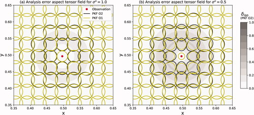
Figure 1 represents the analysis-error aspect tensor fields computed from PKF O1 (yellow ellipses) and PKF O2 (black ellipses); panel (a) shows the result when the observation error standard deviation is set to ${\sigma }^o=1.0,$ while panel (b) shows the same for ${\sigma }^o=0.5.$ To improve the readability, the ellipses are scaled by 0.5. Far from the observation position, the ellipses equal the circles of the initial forecast-error statistics. The impact of the observation modifies the forecast-error aspect tensors at the observation position but also in a vicinity of radius $3L_h$ around the centre. Furthermore, the two experiments illustrate a known effect of the assimilation of observations: the reduction of the forecast error length scale by the observational network (Bouttier, 1994). Both PKF O1 and PKF O2 are able to reproduce this reduction, and this is particularly visible at the centre of the domain where the yellow and black circles superimposed on both panels in Fig. 1 have radii of $0.7L_h$ (panel (a)) and $0.44L_h$ (panel (b)), which are much smaller than the initial circle of radius L_h. However, some differences appear near the observation position: PKF O1 predicts local circles, whereas PKF O2 produces local ellipses. While the forecast-error aspect tensor is isotropic with an isotropy deviation that is identically zero (${\delta }_{\text{iso}}=0$), the isotropy deviation ${\delta }_{\text{iso}}\mathrm{(}\text{PKF}\mathrm{}\mathrm{O}2\mathrm{)}$ computed for PKF O2 shows a peak in the anisotropy centred at the observation location (the grey shading in Fig. 1) with a maximum deviation of 0.13 in panel (a) and 0.3 in panel (b): this production of anisotropy, for PKF O2, is due to the gradient terms in Eq. (13c)(13c) $$\begin{array}{l}{\mathit{g}}^a(\mathit{x})=\frac{V^f(\mathit{x})}{V^a(\mathit{x})}{\mathit{g}}^f(\mathit{x})+\\ \frac{1}{4V^f(\mathit{x})V^a(\mathit{x})}\left[\nabla V^f{(\nabla V^f)}^{\mathrm{T}}\right](\mathit{x})-\\ \frac{1}{V^a(\mathit{x})}\frac{V^f({\mathit{x}}_l)}{V^f({\mathit{x}}_l)+V^o({\mathit{x}}_l)}\\ \left[\nabla ({\sigma }^f{\rho }_{{\mathit{x}}_l}^f){\left(\nabla ({\sigma }^f{\rho }_{{\mathit{x}}_l}^f)\right)}^{\mathrm{T}}\right](\mathit{x})-\\ \frac{1}{4{(V^a(\mathit{x}))}^2}\left[\nabla V^a{(\nabla V^a)}^{\mathrm{T}}\right](\mathit{x}).\end{array}$$(13c) . Note that such a change in the anisotropy is not possible in PKF O1, where the analysis-error aspect tensors are scaled from the forecast error aspect tensors.

Fig. 1. Analysis-error aspect tensor fields for both PKF O2 (black ellipses) and PKF O1 (yellow ellipses): an observation placed at the centre (red dot) is assimilated with an observation error standard deviation of ${\sigma }^o=1.0$ in panel (a) and ${\sigma }^o=0.5$ in panel (b). One in five ellipses is shown here with a zoom on the centre of the domain and a scaling of 0.5 for the ellipse representation. The isotropy deviation ${\delta }_{\text{iso}}$ computed for PKF O2 is superimposed on the fields (the grey shading).

In this experiment, the PKF O2 statistics are identical to the KF statistics (not shown here), which validates the theoretical computation of the metric update Eq. (13c)(13c) $$\begin{array}{l}{\mathit{g}}^a(\mathit{x})=\frac{V^f(\mathit{x})}{V^a(\mathit{x})}{\mathit{g}}^f(\mathit{x})+\\ \frac{1}{4V^f(\mathit{x})V^a(\mathit{x})}\left[\nabla V^f{(\nabla V^f)}^{\mathrm{T}}\right](\mathit{x})-\\ \frac{1}{V^a(\mathit{x})}\frac{V^f({\mathit{x}}_l)}{V^f({\mathit{x}}_l)+V^o({\mathit{x}}_l)}\\ \left[\nabla ({\sigma }^f{\rho }_{{\mathit{x}}_l}^f){\left(\nabla ({\sigma }^f{\rho }_{{\mathit{x}}_l}^f)\right)}^{\mathrm{T}}\right](\mathit{x})-\\ \frac{1}{4{(V^a(\mathit{x}))}^2}\left[\nabla V^a{(\nabla V^a)}^{\mathrm{T}}\right](\mathit{x}).\end{array}$$(13c) . Moreover, the PKF O1, with the simplification Eq. (12)(12) $${\mathit{s}}^a(\mathit{x})\approx \frac{V^a(\mathit{x})}{V^f(\mathit{x})}{\mathit{s}}^f(\mathit{x}),$$(12) , only approximates the KF with an accuracy that depends on the amount of anisotropy introduced during the assimilation. The next section illustrates the PKF in a realistic situation.

4.2. Assessment of the PKF in an heterogeneous test-bed

A first aim of this section is to illustrate the ability of the PKF formulation to provide an accurate approximation of the KF analysis state and its error statistics. For this experiment, the PKF for VLATcov model given by the PKF O2 (Algorithm 2) and its local homogeneous approximation PKF O1 (Algorithm 1) are considered, using the heterogeneous Gaussian Eq. (15)(15) $$\begin{array}{c}{\mathbf{P}}^{\text{he}.\text{gauss}}(V,\mathit{\nu })(\mathit{x},\mathit{y})=\\ \sqrt{V(\mathit{x})V(\mathit{y})}\frac{{\left|{\mathit{s}}_{\mathit{x}}\right|}^{1/4}{\left|{\mathit{s}}_{\mathit{y}}\right|}^{1/4}}{{\left|\frac{1}{2}({\mathit{s}}_{\mathit{x}}+{\mathit{s}}_{\mathit{y}})\right|}^{1/2}}\\ \hspace{0.17em}\text{exp}\hspace{0.17em}\left(-\frac{1}{2}\left|\right|\mathit{x}-\mathit{y}|{|}_{{\left[\frac{1}{2}({\mathit{s}}_{\mathit{x}}+{\mathit{s}}_{\mathit{y}})\right]}^{-1}}^2\right).\end{array}$$(15) as VLATcov model.

The comparison is conducted in a synthetic test-bed that mimics a heterogeneous situation similar to those encountered in real applications. The experiment is organized as follows. First we present the synthetic test-bed where a forecast-error covariance is introduced. Then, a comparison of the KF and PKF analysis steps is made.

4.2.1. Synthetic anisotropic test-bed

In order to consider a realistic forecast-error aspect tensor field, an isotropic tensor field of length scale of $4\delta x\approx 0.03$ has been deformed by a non-divergent flow, shown in Fig. 2(a) and integrated from t = 0 to t = 3. The resulting aspect tensor field ${\mathit{s}}^f,$ is represented by some ellipses superimposed to the isotropy deviation (in Fig. 2b) and to the isotropic length-scale (in Fig. 2c).

Fig. 2. Illustration of the non-divergent velocity field (a) whose integration from 0 to 3 has been used to transforms an isotropic aspect tensor field into an anisotropic one taken as the forecast error aspect tensor field. The ellipses in panel (b) and (c) show some of the forecast error aspect tensors, superimposed with the diagnosis of the deviations from isotropy (b) (0 indicates an isotropic tensor and 1 indicates a purely anisotropic tensor) and the isotropic length scale normalized by the grid spacing (c). The ellipses in the two panels (b) and (c), are the same, and the panels differ only by the shading.

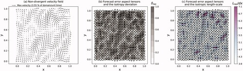
The forecast-error aspect tensor field shows strong anisotropies. The field of the isotropy deviation (Eq. (8)(8) $${\delta }_{\text{iso}}=\frac{1}{d-1}\left|\right||\mathit{s}{({\mathit{s}}_{\text{iso}})}^{-1}-{\mathbf{I}}_d|\left|\right|,$$(8) ) ranges from 0.003 to 0.95 with an average of 0.58, which means that all types of situations are encountered from nearly isotropic to nearly singular tensors (see panel (b) in Fig. 2). Further, the isotropic length scale (Eq. (9)(9) $$L_{\text{iso}}={(\text{Tr}(\mathit{s})/d)}^{1/2},$$(9) ) normalized by the grid spacing varies from 3.9 to 7 (see panel (c) in Fig. 2), which is in agreement with the range of variations observed in geophysics, see e.g. Wu et al. (2002), Belo Pereira and Berre (2006) and Pannekoucke and Massart (2008). With these setting, the forecast error aspect tensor field is relevant because it is similar to various typical situations encountered in the realm of geophysical data assimilations.

Note that in real applications, if the PKF has not been considered for the forecast step, the variance and the aspect tensor fields can be diagnosed from an ensemble of forecasts, ${\left\{{\mathcal{X}}^f{}_k\right\}}_{k\in [1,N]}$ (at a given time), where N is the number of members. Hence, the estimator of the variance is (17) $$\widehat{V^f}(x)=\frac{1}{N-1}\sum _{k=1}^N{\left({\mathcal{X}}^f{}_k(x)-\overline{{\mathcal{X}}^f}(x)\right)}^2,$$(17) where $\overline{{\mathcal{X}}^f}=\frac{1}{N}{\sum }_{k=1}^N{\mathcal{X}}^f{}_k$ is the ensemble average. The metric tensor, defined from Eq. (6)(6) $$g_{ij}^f(\mathit{x})=\mathbb{E}\left[{\partial }_{x^i}\left(\frac{{\mathbf{\epsilon }}^f}{{\sigma }^f}\right){\partial }_{x^j}\left(\frac{{\mathbf{\epsilon }}^f}{{\sigma }^f}\right)\right](\mathit{x}),$$(6) , is estimated by (18) $$\widehat{g_{ij}^f}(x)=\frac{1}{N}\sum _{k=1}^N{\partial }_i{\widetilde{{\mathit{\epsilon }}^f}}_k(x){\partial }_j{\widetilde{{\mathit{\epsilon }}^f}}_k(x),$$(18) where ${\widetilde{{\mathit{\epsilon }}^f}}_k=\frac{1}{\sqrt{\widehat{V^f}}}({\mathcal{X}}^f{}_k-\overline{{\mathcal{X}}^f})$ is the normalized error. When the PKF is implemented in an assimilation cycle, the forecast error variance and the metric tensor fields are propagated over the forecast time step, as in standard KF, from the values obtained at the previous analysis time.

For the latter numerical experiments, the forecast-error covariance matrix ${\mathbf{P}}^f,$ is defined as the covariance matrix based on a diffusion equation (Weaver and Courtier, 2001) with the diffusion tensors set as $\frac{1}{2}{\mathit{s}}^f$ (Pannekoucke and Massart, 2008; Mirouze and Weaver, 2010). In particular, ${\mathbf{P}}^f$ has been stored explicitly as follows. Each column j of the matrix is associated with one of the 19881 grid-points, ${\mathit{x}}_j,$ and the column is computed as the time integration of the Dirac positioned at ${\mathit{x}}_j,$ δ_j, by the heterogeneous diffusion equation computed from time 0 to time 1/2 i.e. $e^{\frac{1}{2}\nabla ·\left(\frac{1}{2}{\mathit{s}}^f\nabla \right)}{\delta }_j.$ Then, the resulting matrix is normalized so that the variance is 1.0, which leads to ${\mathbf{P}}^f.$

In the experiment conducted here, we use the heterogeneous Gaussian VLATcov model ${\mathbf{P}}^{\text{he}.\text{gauss}}(1.,{\mathit{s}}^f)$ to approximate ${\mathbf{P}}^f.$ Figure 3 illustrates the correlation functions of ${\mathbf{P}}^f$ (a) and ${\mathbf{P}}^{\text{he}.\text{gauss}}(1.,{\mathit{s}}^f)$ (b) set from the aspect tensor in Fig. 2. For the sake of simplicity, only 1 in 20 correlation functions are shown and each function is represented by level sets of the iso-correlation values of 0.5, 0.7 and 0.9, coloured from light to dark grey. For each point selected for the illustration, the correlation function presents a non-elliptic anisotropic shape, and the correlation functions vary from one point to another. The correlation functions produced by the heterogeneous Gaussian are very similar to the one of the reference ${\mathbf{P}}^f.$

Fig. 3. Prescribed forecast-error correlation functions as specified from a diffusion formulation (a), and the heterogeneous Gaussian correlations (b), and defined from the aspect tensor field Fig. 2. The level sets of the iso-correlations $\{0.5,0.7,0.9\}$ are represented from light to dark grey.

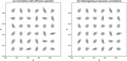
This proximity is confirmed by the computation of the relative error $\left|\right|{\mathbf{P}}^{\text{he}.\text{gauss}}(V^f,{\mathit{\nu }}^f)-{\mathbf{P}}^f\left|\right|/\left|\right|{\mathbf{P}}^f\left|\right|=7.6\%,$ where $\left|\right|\mathbf{U}\left|\right|=\sqrt{\text{Tr}(\mathbf{U}{\mathbf{U}}^{\mathrm{T}})},$ for any $\mathbf{U}$ denotes the Frobenius norm of the matrix. Therefore, the correlation functions based on the heterogeneous Gaussian function are an accurate approximation of the correlation functions modelled from the diffusion equation.

The next section describes the details of the assimilation experiment and how the KF analysis uncertainty is performed to provide a reference for a comparison with the PKF algorithms.

4.2.2. Details of the assimilation experiment and the computation of the KF analysis statistics

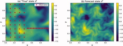
The true state ${\mathcal{X}}^t$ considered here is shown in Fig. 4(a), including the observational network (the red dots). This network presents a contrast between the left and right parts of the domain, where the network is more dense in the left part. In the left part, 1 in 15 grid points are depicted along the zonal and meridional directions. In the right part, a dense path mimics a flight corridor with two observed grid points for each observed zonal position. In the numerical experiment, the observational error covariance matrix is set to $\mathbf{R}={({\sigma }^o)}^2{\mathbf{I}}_p$ with a standard deviation of ${\sigma }^o=1.0.$ An observation vector is generated such that ${\mathcal{Y}}^o=\mathbf{H}{\mathcal{X}}^t+{\mathit{\epsilon }}^o,$ where ${\mathit{\epsilon }}^o={\mathbf{R}}^{1/2}{\zeta }_p,$ ζ_p is a sample of the Gaussian law with zero mean and a covariance matrix ${\mathbf{I}}_p$ and the superscript ${}^{1/2}$ denotes the square-root operator for symmetric positive-definite matrices. A particular forecast state was generated from the true state in accordance with the forecast error statistics (Fig. 4b). This forecast state is obtained as ${\mathcal{X}}^f={\mathcal{X}}^t+{\mathit{\epsilon }}^f,$ where ${\mathit{\epsilon }}^f={\mathbf{P}}^f{}^{1/2}{\zeta }_n$ and ζ_n is a Gaussian sample with zero mean and a covariance matrix ${\mathbf{I}}_n.$

Fig. 4. The (a) true ${\mathcal{X}}^t$ and (b) forecast ${\mathcal{X}}^f$ states considered in the experiment with the observational network (the red dots in panel (a)) of 80 observed positions.

The Kalman filter analysis step Eq. (1)(1a) $${\mathcal{X}}^a={\mathcal{X}}^f+\mathbf{K}\left({\mathcal{Y}}^o-\mathbf{H}{\mathcal{X}}^f\right),$$(1a) has been computed explicitly from its matrix formulation: each matrix is of size $(19881,19881)$ which represent 3.2 GB of memory. The CPU time for the computation of the gain matrix $\mathbf{K}$ is 0.96 seconds (on an Intel Core i7-7820HQ CPU at 2.90 GHz x 8), the analysis state is performed in 0.001 seconds and the analysis-error covariance matrix requires 101 seconds. In particular, the analysis-error covariance matrix ${\mathbf{P}}^a$ is exactly known (to within the numerical error due to the precision of the machine), and it can be used to assess the quality of the PKF approach.

4.2.3. The KF analysis versus its PKF approximation

To compare the analyses, emphasis is given to the analysis increment, which is defined as the difference $d{\mathcal{X}}^a={\mathcal{X}}^a-{\mathcal{X}}^f.$ The three analysis increments, $d{\mathcal{X}}^a(KF),d{\mathcal{X}}^a(\mathit{PKF}O1)$ and $d{\mathcal{X}}^a(\mathit{PKF}O2),$ are shown in Fig. 5.

Fig. 5. Analysis increments for (a) the KF, (b) PKF O1 and (c) PKF O2.

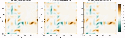
All analysis increments provide a correction of the forecast in the vicinity of the observations. This correction is a combination of the different forecast error correlation functions, some of which are illustrated in Fig. 3, resulting in a very complex field. Due to the heterogeneity of the observation network between the left and right sides of the domain, the analysis increments are nearly zero on the right side, except in the neighbourhood of the tracks.

This similarity between the analysis increments was confirmed via a quantitative diagnosis. Compared to the KF analysis increment, the relative errors of the analysis increments computed from PKF O1 and PKF O2 are 8.9% and 9.3%, respectively (see Table 1, first column). A more attentive examination of Fig. 5 indicates that the PKF O1 (panel b) and the PKF O2 (panel c) are able to produce curved patterns that are connected to the underlying vortices of the flow and very similar to the patterns produced by the KF (panel a).

Table 1. Relative error for the analysis increment and error statistics with the KF as the reference.

PKF	$\frac{\left|\right|\delta {\mathcal{X}}^a(.)-\delta {\mathcal{X}}^a(KF)\left|\right|}{\left|\right|\delta {\mathcal{X}}^a(KF)\left|\right|}$	$\frac{\left|\right|V^a(.)-V^a(KF)\left|\right|}{\left|\right|V^a(KF)\left|\right|}$	$\frac{\sum _{\mathit{x}}\left|\right|{\mathbf{s}}_{\mathit{x}}^a(.)-{\mathbf{s}}_{\mathit{x}}^a(KF)\left|\right|}{\sum _{\mathit{x}}\left|\right|{\mathbf{s}}_{\mathit{x}}^a(KF)\left|\right|}$
O1	8.91%	1.26%	9.14%
O2	9.35%	1.01%	8.86%

$\left|\right|·\left|\right|$ stands for the L² norm. The results have been approximated to the hundredth of a percent.

Note that, since PKF O1 and PKF O2 produce the same analysed fields in the case a unique observation is assimilated with the same background statistics, the difference in analysis increments must come from the fact that the two algorithms are cycled sequentially over all the observations.

Therefore, this experiment indicates that the PKF algorithms are able to estimate the KF analysis. However, the complexity of PKF O2 compared to PKF O1 does not provide any clear advantage.

The analysis error variance is examined in the next section.

4.2.4. KF analysis error variance versus its PKF approximation

The analysis-error variance fields are shown in Fig. 6. The KF analysis variance field is obtained as the diagonal of the fully computed analysis-error covariance matrix ${\mathbf{P}}^a$ in Eq. (1b)(1b) $${\mathbf{P}}^a=({\mathbf{I}}_n-\mathbf{KH}){\mathbf{P}}^f,$$(1b) .

Fig. 6. Analysis-error variance fields for the KF (a), the PKF O1 (b), and the PKF O2 (c).

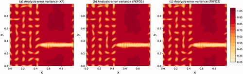
The analysis-error variance fields are all similar, showing a strong variance reduction in the vicinity of each observation. This reduction of the error variance is maximal where the observation network is dense, e.g. on the right side of the domain along the simulated flight path, where the reduction is 75% of the initial forecast error variance. Relative to the KF analysis error variance field (see Table 1, second column), all the error variance fields are very close to the KF reference with relative errors on the order of 1%. In this case, PKF O2 provides very little improvement compared to PKF O1 with a relative error of 1.0% versus 1.2%. Note that, analysis-error variance fields estimated from EnKF methods are often polluted by sampling noise. Here, because no ensemble is used in the PKF formulations, no fluctuation is visible in the PKF panels.

Therefore, in this experiment, the PKF O1 and PKF O2 formulations are shown to be capable of computing an accurate approximation of the analysis error variance field.

We end the comparison by considering the analysis error correlation anisotropy.

4.2.5. KF analysis-error aspect tensor versus the PKF approximation

The diagnosis of the KF analysis-error local aspect tensors relies on the computation of the local metric tensors. In the present experiment, the local metric tensors are diagnosed from the fully computed analysis error covariance matrix Eq. (1b)(1b) $${\mathbf{P}}^a=({\mathbf{I}}_n-\mathbf{KH}){\mathbf{P}}^f,$$(1b) : for each position $\mathit{x},{\mathit{g}}^a(\mathit{x})$ is obtained from the analysis error correlation function ${\rho }^a(\mathit{x},·)$ by Eq. (4)(4) $$g_{ij}^f(\mathit{x})=-{\partial }_{x^i{x}^j}^2{\rho }^f{(\mathit{x},\mathit{y})}_{|\mathit{y}=\mathit{x}},$$(4) . Then, the diagnosis of the local analysis-error aspect tensor for the KF is ${\mathit{s}}^a(\mathit{x})={({\mathit{g}}^a(\mathit{x}))}^{-1}.$ The KF analysis-error aspect tensors (not shown here) are similar to the one of the forecast, where some of the ellipses are shown in Fig. 2, except in the vicinity of the observations due to the assimilation process.

The analysis-error aspect tensors obtained from the PKF are similar to the KF. This is confirmed quantitatively by taking the ratio $\frac{\sum _{\mathit{x}}\left|\right|{\mathit{s}}_{\mathit{x}}^a(\mathit{PKF})-{\mathit{s}}_{\mathit{x}}^a(KF)\left|\right|}{\sum _{\mathit{x}}\left|\right|{\mathit{s}}_{\mathit{x}}^a(KF)\left|\right|}$ as a global indicator of the relative error to the KF (see Table 1, third column): it appears that all formulations are able to approximate the KF analysis-error aspect tensors with an error of the order of 10%, the PKF O2 provides the best approximation here, with a relative error of 8.9%.

To evaluate the results obtained from the different PKF approximations, a representation of ellipses, as given in Fig. 2, is informative but difficult to show in details. In place of the ellipses, the comparison is made by looking at the scalar field of the relative variation of the local isotropic length scales, Eq. (9)(9) $$L_{\text{iso}}={(\text{Tr}(\mathit{s})/d)}^{1/2},$$(9) , which is defined as (19) $$r_{\text{iso}}^{af}=\frac{L_{\text{iso}}^a-L_{\text{iso}}^f}{L_{\text{iso}}^f}.$$(19)

This relative variation depicts the evolution of the spread before and after the assimilation of the observations. The $r_{\text{iso}}^{af}$ fields for the KF and PKF formulations are shown in Fig. 7.

Fig. 7. Relative variation of the isotropic length scale, $r_{\text{iso}}^{af}=\frac{L_{\text{iso}}^a-L_{\text{iso}}^f}{L_{\text{iso}}^f},$ for the KF (a), the PKF O1 (b), and the PKF O2 (c). The white colour indicates values larger than those within the colour range.

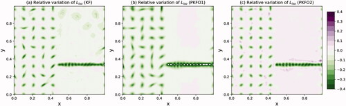
All the analysis-error aspect tensor fields show a reduction of the isotropic length scale in the vicinity of each observation, which is a known consequence of the assimilation of observations (Bouttier, 1994). However, the reduction can also be surrounded by an augmentation of the correlation spread, as noted in P16 who have observed an overshoot of analysis-error correlation length-scale in the vicinity of the position of an assimilated observation (note that this kind of overshoot is also visible and discussed in Sec. 5.2). Such an increase in the correlation spread appears moderately in the KF statistics near the simulated flight tracks and is reproduced by PKF O2 e.g. the purple shading visible on the right side of Fig. 7c for the ordinates $y\approx 0.3$ and $y\approx 0.4;$ this is also present in Fig. 7a but less visible by eyes. The local increase in the correlation spread has its origin in the contribution of the gradients in the last three terms of the error analysis metric tensor in Eq. (13c)(13c) $$\begin{array}{l}{\mathit{g}}^a(\mathit{x})=\frac{V^f(\mathit{x})}{V^a(\mathit{x})}{\mathit{g}}^f(\mathit{x})+\\ \frac{1}{4V^f(\mathit{x})V^a(\mathit{x})}\left[\nabla V^f{(\nabla V^f)}^{\mathrm{T}}\right](\mathit{x})-\\ \frac{1}{V^a(\mathit{x})}\frac{V^f({\mathit{x}}_l)}{V^f({\mathit{x}}_l)+V^o({\mathit{x}}_l)}\\ \left[\nabla ({\sigma }^f{\rho }_{{\mathit{x}}_l}^f){\left(\nabla ({\sigma }^f{\rho }_{{\mathit{x}}_l}^f)\right)}^{\mathrm{T}}\right](\mathit{x})-\\ \frac{1}{4{(V^a(\mathit{x}))}^2}\left[\nabla V^a{(\nabla V^a)}^{\mathrm{T}}\right](\mathit{x}).\end{array}$$(13c) .

No increase of the correlation spread appears in Fig. 7b for the PKF O1 (no purple shading near the flight tracks), whose the update by Eq. (11)(11) $${\mathit{g}}^a(\mathit{x})\approx \frac{V^f(\mathit{x})}{V^a(\mathit{x})}{\mathit{g}}^f(\mathit{x}),$$(11) is without spatial derivatives. For the PKF O1, the spread of analysis-error aspect tensors can only decrease from the forecast ones because $V^a/V^f\le 1,$ and without change in the anisotropy (as shown in Sec. 4.1).

In addition, compared to Fig. 7a and 7c, PKF O1 produces larger patterns of isotropic length-scale reductions near each observation: the gradient terms in Eq. (13c)(13c) $$\begin{array}{l}{\mathit{g}}^a(\mathit{x})=\frac{V^f(\mathit{x})}{V^a(\mathit{x})}{\mathit{g}}^f(\mathit{x})+\\ \frac{1}{4V^f(\mathit{x})V^a(\mathit{x})}\left[\nabla V^f{(\nabla V^f)}^{\mathrm{T}}\right](\mathit{x})-\\ \frac{1}{V^a(\mathit{x})}\frac{V^f({\mathit{x}}_l)}{V^f({\mathit{x}}_l)+V^o({\mathit{x}}_l)}\\ \left[\nabla ({\sigma }^f{\rho }_{{\mathit{x}}_l}^f){\left(\nabla ({\sigma }^f{\rho }_{{\mathit{x}}_l}^f)\right)}^{\mathrm{T}}\right](\mathit{x})-\\ \frac{1}{4{(V^a(\mathit{x}))}^2}\left[\nabla V^a{(\nabla V^a)}^{\mathrm{T}}\right](\mathit{x}).\end{array}$$(13c) have the effect of localizing the reduction of the spread of the KF and PKF O2 in a smaller vicinity than that of PKF O1. Moreover, the minimum reduction of the isotropic length scale appears to be smaller than the true reduction of the KF and that proposed by PKF O2; this is especially visible for the simulated flight tracks.

To summarize the comparison of the analysis-error aspect tensors in this example, we conclude that the PKF is capable of providing an accurate approximation of the KF analysis-error aspect tensors.

4.3. Illustration of assimilation cycles

While this contribution is focused on the analysis step, a simple illustration of the PKF assimilation over several cycles is now introduced.

4.3.1. Setting of the experiment

We consider the 2D transport of a scalar field $\mathcal{X}$ by the stationary wind field $\mathbf{u}={\mathbf{u}}^0+\mathbf{u}\prime ,$ where ${\mathbf{u}}^o=(0.04,0.04)$ is a mean flow and $\mathbf{u}\prime$ is the non-divergent fluctuation shown in Fig. 2a. The advection time associated to the mean flow is $L/\left|\right|{\mathbf{u}}^o\left|\right|\approx 17.6,$ and the maximum magnitude of $\mathbf{u}\prime$ is 62% of $\left|\right|{\mathbf{u}}^o\left|\right|.$ Hence, the transport equation reads (20) $${\partial }_t\mathcal{X}+\mathbf{u}·\nabla \mathcal{X}=0,$$(20) integrated over the 2D domain described in the previous section i.e. ${[0,L)}^2,$ with L = 1, and discretized with 141 points along each directions which represents n = 19,881 grid points, and $\delta x=\delta y\approx 0.007.$

The cycled assimilation experiment relies on a simulated experiment where a reference state at t = 0, ${\mathcal{X}}^t{}_0,$ evolves in time with Eq. (20)(20) $${\partial }_t\mathcal{X}+\mathbf{u}·\nabla \mathcal{X}=0,$$(20) , and is observed as each $\Delta t=0.5$ at the observational network shown in Fig. 4a. In this experiment, ${\mathcal{X}}^t{}_0$ is the isotropic Gaussian function positioned at the center of the domain and of scale parameter $10\delta x.$ The observations at a time $t_q=q\Delta t,$ are generated as ${\mathcal{Y}}^o{}_q=\mathbf{H}{\mathcal{X}}^t{}_q+{\mathit{\epsilon }}^o{}_q,$ where ${\mathcal{X}}^t{}_q={\mathcal{X}}^t(t_q)$ and where ${\mathit{\epsilon }}^o{}_q$ is a sample of the Gaussian $\mathcal{N}(0,{\mathbf{I}}_p)$ where p = 80 is the number of observation in the network. With this setting, the observational error variance is $V^o=1.$ The initial uncertainty is defined as the Gaussian of mean ${\mathcal{X}}^f{}_0,$ that is set to the zero vector, and of covariance matrix ${\mathbf{P}}_0^f$ the isotropic covariance Eq. (16)(16) $${\mathbf{P}}^f(L_h)(\mathit{x},\mathit{y})=\hspace{0.17em}\text{exp}\hspace{0.17em}\left(-\frac{1}{2L_h^2}\left|\right|\mathit{x}-\mathit{y}|{|}^2\right),$$(16) with the length-scale $L_h=4\delta x\approx 0.03$ i.e. $V_0^f=1$ and ${\mathit{s}}_0^f=L_h^2{\mathbf{I}}_2.$

The aim of the experiment is to compare the results given by the parametric the PKF O1 and PKF O2, versus the Kalman filter, over 19 assimilation cycles, starting from an analysis step at t = 0 and ending by the assimilation at time $t_{19}=9$ (the flow covers almost half of the domain during the period $[0,9]$). Thus, three experiments of assimilation cycles are performed considering respectively the KF, the PKF O1 and the PKF O2 at the assimilation times t_q.

The VLATcov model considered for the PKF is the heterogeneous Gaussian, Eq. (15)(15) $$\begin{array}{c}{\mathbf{P}}^{\text{he}.\text{gauss}}(V,\mathit{\nu })(\mathit{x},\mathit{y})=\\ \sqrt{V(\mathit{x})V(\mathit{y})}\frac{{\left|{\mathit{s}}_{\mathit{x}}\right|}^{1/4}{\left|{\mathit{s}}_{\mathit{y}}\right|}^{1/4}}{{\left|\frac{1}{2}({\mathit{s}}_{\mathit{x}}+{\mathit{s}}_{\mathit{y}})\right|}^{1/2}}\\ \hspace{0.17em}\text{exp}\hspace{0.17em}\left(-\frac{1}{2}\left|\right|\mathit{x}-\mathit{y}|{|}_{{\left[\frac{1}{2}({\mathit{s}}_{\mathit{x}}+{\mathit{s}}_{\mathit{y}})\right]}^{-1}}^2\right).\end{array}$$(15) . For this covariance model, a forecast step of the PKF O1 and PKF O2, consists in predicting the mean ${\mathcal{X}}^f{}_{q+1},$ the variance field $V_{q+1}^f$ and the aspect tensor field ${\mathit{s}}_{q+1}^f$ from their respective analysis values at t_q i.e. ${\mathcal{X}}^a{}_q,V_q^a$ and ${\mathit{s}}_q^a.$ For the transport dynamics, this prediction is performed by the time integration, from t_q to $t_{q+1},$ of the system (21a) $${\partial }_t{\mathcal{X}}^f+\mathbf{u}·\nabla {\mathcal{X}}^f=0,$$(21a) (21b) $${\partial }_t{V}^f+\mathbf{u}·\nabla V^f=0,$$(21b) (21c) $${\partial }_t{\mathit{s}}^f+\mathbf{u}·\nabla {\mathit{s}}^f=\left(\nabla \mathbf{u}\right){\mathit{s}}^f+{\mathit{s}}^f{\left(\nabla \mathbf{u}\right)}^T+\eta {\nabla }^2{\mathit{s}}^f,$$(21c) where these equations correspond to the dynamics of, the mean in Eq. (21a)(21a) $${\partial }_t{\mathcal{X}}^f+\mathbf{u}·\nabla {\mathcal{X}}^f=0,$$(21a) , the forecast-error variance in Eq. (21b)(21b) $${\partial }_t{V}^f+\mathbf{u}·\nabla V^f=0,$$(21b) and the forecast-error aspect tensor in Eq. (21c)(21c) $${\partial }_t{\mathit{s}}^f+\mathbf{u}·\nabla {\mathit{s}}^f=\left(\nabla \mathbf{u}\right){\mathit{s}}^f+{\mathit{s}}^f{\left(\nabla \mathbf{u}\right)}^T+\eta {\nabla }^2{\mathit{s}}^f,$$(21c) . Equation (21) corresponds to the true uncertainty dynamics (Cohn, 1993; Pannekoucke et al., 2016, 2018a), plus a slight additional diffusion of coefficient $\eta =\delta x^2.$ This diffusion has been introduced in order to regularize strong anisotropy during the time evolution.

The transport Eq. (20)(20) $${\partial }_t\mathcal{X}+\mathbf{u}·\nabla \mathcal{X}=0,$$(20) being linear, we denote by ${\mathbf{M}}_{q+1\leftarrow q}$ its linear propagator. Hence, the KF predictions of the covariance error matrix read (22) $${\mathbf{P}}_{q+1}^f={\mathbf{M}}_{q+1\leftarrow q}{\left({\mathbf{M}}_{q+1\leftarrow q}{\mathbf{P}}_q^a\right)}^T.$$(22)

Because of the numerical cost needed to perform Eq. (22)(22) $${\mathbf{P}}_{q+1}^f={\mathbf{M}}_{q+1\leftarrow q}{\left({\mathbf{M}}_{q+1\leftarrow q}{\mathbf{P}}_q^a\right)}^T.$$(22) , we approximated the dynamics by considering an EnKF of N_e = 1000 members. The assimilation steps are also performed by using an ensemble, here an ensemble transform method has been considered (Hunt et al., 2007). The ensemble at time 0, ${({\mathcal{X}}^f{}_{0,k})}_{k\in [1,N_e]},$ has been generated as follows: each member is set as ${\mathcal{X}}^f{}_{0,k}={\mathcal{X}}^f{}_0+{\mathbf{P}}_0^f{}^{1/2}{\eta }_k$ where η_k is a sample of the Gaussian $\mathcal{N}(0,{\mathbf{I}}_n),$ with n = 19,881 being the number of grid points. The diagnosis of the analysis-error variance and aspect tensor fields are performed from the ensemble estimation detailed, respectively, in Eqs. (17)(17) $$\widehat{V^f}(x)=\frac{1}{N-1}\sum _{k=1}^N{\left({\mathcal{X}}^f{}_k(x)-\overline{{\mathcal{X}}^f}(x)\right)}^2,$$(17) and (18)(18) $$\widehat{g_{ij}^f}(x)=\frac{1}{N}\sum _{k=1}^N{\partial }_i{\widetilde{{\mathit{\epsilon }}^f}}_k(x){\partial }_j{\widetilde{{\mathit{\epsilon }}^f}}_k(x),$$(18) , and applied to the ensemble of analysis. In particular, a localization of the forecast-error covariance has been considered within the assimilation, using the compactly-supported correlation Eq. (4.10) of Gaspari and Cohn (1999), with a localization length-scale defined at t_q as the spatial average of $3\sqrt{L_{q,x}^f{L}_{q,y}^f}$ where $L_{q,x}=\sqrt{{\mathit{s}}_{q,xx}^f(t_q)}$ and $L_{q,y}=\sqrt{{\mathit{s}}_{q,yy}^f(t_q)}$ are the correlation length-scale along each directions, computed at times t_q.

In the numerical simulation, the dynamics Eqs. (20)(20) $${\partial }_t\mathcal{X}+\mathbf{u}·\nabla \mathcal{X}=0,$$(20) and (21(21a) $${\partial }_t{\mathcal{X}}^f+\mathbf{u}·\nabla {\mathcal{X}}^f=0,$$(21a) ) have been spatially discretized with a finite difference method, where the first order spatial derivatives are computed with a centered scheme (consistent at the order $\delta x^2$). For the time integration, a fourth-order Runge-Kutta scheme, of time step dt = 0.01, has been used. Note that, to perform an ensemble prediction of the error covariance matrix with the EnKF, 1000 forecasts of Eq. (20)(20) $${\partial }_t\mathcal{X}+\mathbf{u}·\nabla \mathcal{X}=0,$$(20) are computed, while the PKF only needs a single forecast of Eq. (21)(21a) $${\partial }_t{\mathcal{X}}^f+\mathbf{u}·\nabla {\mathcal{X}}^f=0,$$(21a) .

4.3.2. Comparison from the numerical simulation

We compare now the analysis increment (see Fig. 8), the analysis-error variance field (see Fig. 9) and the relative variation of the isotropic analysis-error length-scale with respect to the initial isotropic length-scale L_h, $r_{\mathit{iso}}^{ah}=\frac{L_{\text{iso}}^a-L_h}{L_h}$ (see Fig. 10), resulting from the PKF O1 and the PKF O2 assimilation cycles, versus the EnKF (the proxy for the true KF solution). These results show the analysis-error statistics at times 0, 3.5 and 9, while the relative error between the PKF results and the EnKF is shown for each assimilation times in Fig. 11. As for the assimilation experiment, the only difference between the PKF O1 and PKF O2 is the update of the anisotropy; the prediction steps are performed by the same dynamics, Eq. (21)(21a) $${\partial }_t{\mathcal{X}}^f+\mathbf{u}·\nabla {\mathcal{X}}^f=0,$$(21a) . In this simulation, the PKF O2 fails at time 4. because an aspect tensor became non-positive with a negative determinant.

Fig. 8. Analysis increments resulting from the assimilation cycles using an EnKF of 1000 members (left column), the PKF O1 (middle column) and the PKF O2 (right column). Only the results at time 0 (top line), 3.5 (middle line) and 9 (bottom line) are shown, while an assimilation is performed each $\Delta t=0.5$ which represents 19 assimilation cycles. PKF O2 fails after $t=4.$

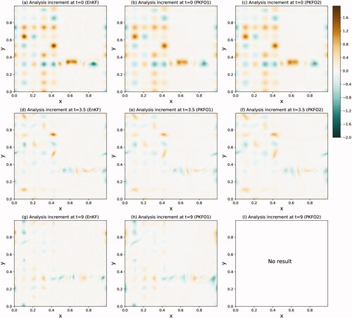
Fig. 9. Same as for Fig. 8 but for the analysis-error variance fields. In panel (a), the white colour indicates values larger than those of the colour range.

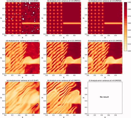
Fig. 10. Same as for Fig. 8 but for the relative variation of the isotropic analysis-error length-scale with respect to the initial isotropic length-scale $L_h=4\delta x,r_{\mathit{iso}}^{ah}=\frac{L_{\text{iso}}^a-L_h}{L_h}.$

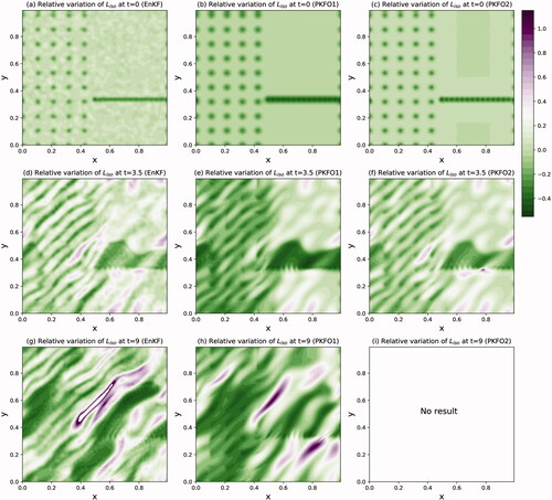
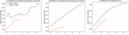
Fig. 11. Relative error of the EnKF and of the PKF O2 vs. the PKF O1 solution computed for the analysis state (a), the analysis-error variance field (b) and the analysis-error isotropic length-scale field (c). An assimilation is performed each $\Delta t=0.5.$

At first sight, the PKF implementations are able to reproduce the EnKF solution: the analysis-increment, the variance field and the isotropic length-scale are very similar from one assimilation experiment to another. A more complete evaluation is now detailed.

We first consider the results obtained at time 0. Compared with the full matrix computation of the previous sections Secs. 4.1 and 4.2, this time, the EnKF approximation of the KF makes appear a sampling noise. This sampling noise is particularly visible on the analysis-error variance, that should be exactly 1 far from the observations, but that fluctuates here around 1: in Fig. 9a the values larger than 1.1 are in white. More precisely, we observed that the ensemble estimation of the forecast-error variance field at 0, $V_0^f,$ fluctuates from 0.83 to 1.2 around the mean 1.0 and with a standard-deviation of 0.044; in accordance with the theoretical magnitude of the estimation error, $\sqrt{\frac{2}{N_e}}{V}_0^f$ (central limit theorem), which implies a relative error of 4.4% for $V_0^f=1.0$ and an ensemble size of N_e = 1000. The magnitude of the fluctuations explains the relative error observed at t = 0, where the difference between the EnKF and the PKF is 5.6% (5.5%) for the PKF O1 (the PKF O2) (see Fig. 11b): this amount of error comes from the sampling noise plus an error due to the PKF itself (1% of error according to Table 1).

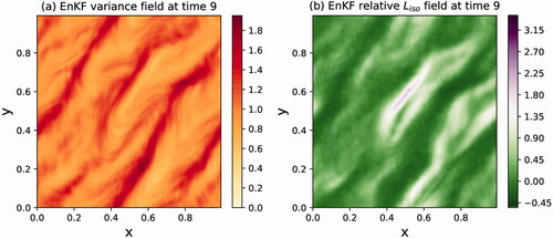
Before considering the variation of the various diagnostics with time, we first evaluate the ability of the EnKF to reproduce the true KF dynamics in this framework. Note that the dynamics of the KF statistics evolves by Eq. (21)(21a) $${\partial }_t{\mathcal{X}}^f+\mathbf{u}·\nabla {\mathcal{X}}^f=0,$$(21a) without the diffusion (η = 0): this is an exact result for the transport dynamics (Cohn, 1993; Pannekoucke et al., 2018a, 2020). As a consequence, an initially homogeneous variance field should be stationary: the forecast-error variance field should be equal to its initial constant value. This stationarity property is tested by considering an ensemble of 1000 forecasts over the window $[0,9],$ without assimilation, and the statistics are shown in Fig. 12. In this pure ensemble forecast experiment, the spatial average of the forecast-error variance, shown at time 9 in Fig. 12a, is 1.03 which represent a slight increases of 3% of the averaged variance value: this is in accordance with the stationarity of homogeneous variance field in the transport dynamics. However, the forecast-error variance field becomes heterogeneous over the time. For instance, at time 9 (see Fig. 12a), the variance field varies from 0.6 to 1.9 with a standard deviation of the spatial variations of 0.2; while the KF predicts a constant variance equal to 1—to within the sampling noise in this ensemble experiment. But fluctuations of magnitude 0.2 are much larger than the fluctuation of a sampling noise that has shown to be 0.044 in this situation. Hence, the heterogeneity cannot be explained from a sampling noise, and should result from the effect of a model error. Following Pannekoucke et al. (2020), the understanding of the discretization error can be deduced from the so called modified equation associated with a numerical scheme, that is the differential equation verified by the numerical solution (Warming and Hyett, 1974). For Eq. (20)(20) $${\partial }_t\mathcal{X}+\mathbf{u}·\nabla \mathcal{X}=0,$$(20) considered here, the modified equation, only associated with the spatial discretization at the second order in δx and δy, reads (23) $${\partial }_t\chi +\mathbf{u}·\nabla \chi =-\frac{\delta x^{2}u}{6}{\partial }_x^3\chi -\frac{\delta y^{2}v}{6}{\partial }_y^3\chi ,$$(23) where $\mathbf{u}=(u(x,y),v(x,y)).$ Since a fourth-order Runge-Kutta scheme implies a fourth-order error in δt, that can be neglected compared to the second-order error in space, the dynamics of the numerical solution of Eq. (20)(20) $${\partial }_t\mathcal{X}+\mathbf{u}·\nabla \mathcal{X}=0,$$(20) is well approximated by Eq. (23)(23) $${\partial }_t\chi +\mathbf{u}·\nabla \chi =-\frac{\delta x^{2}u}{6}{\partial }_x^3\chi -\frac{\delta y^{2}v}{6}{\partial }_y^3\chi ,$$(23) . Hence the model error is mainly due to the spatial discretization. Here, Eq. (23)(23) $${\partial }_t\chi +\mathbf{u}·\nabla \chi =-\frac{\delta x^{2}u}{6}{\partial }_x^3\chi -\frac{\delta y^{2}v}{6}{\partial }_y^3\chi ,$$(23) makes appear additional processes in its right hand-side, given by a third order spatial derivative (a dispersive term). From the computation of the PKF dynamics (Pannekoucke et al., 2018a), the effect of a third-order spatial derivative (like every spatial derivative of order strictly larger than 1) is to introduce a coupling between the forecast-error variance and aspect tensor fields during the time evolution. In this case (not detailed), the dynamics of the variance is mainly a conservation law, that conserves the spatial average but may breaks the homogeneity of an initially constant field because of the heterogeneity of the anisotropy field. The coupling appears here by a reorganization of the variance field which becomes larger over areas of short isotropic length-scale (compare panels (a) and (b) in Fig. 12).

Fig. 12. Forecast-error variance (a) and relative isotropic length-scale (b) resulting from an ensemble of 1000 forecasts, integrated from time 0 to 9 without assimilation.

This interlude shows that it is can be difficult to evaluate the PKF from a comparison with an EnKF taken as a proxy for the true KF, because the EnKF also suffers from defects. Hence, for the quantitative evaluation, we chose to compare the PKF and the EnKF by measuring the relative error with respect to the PKF O1. Taking the PKF O1 as the reference for the score, also facilitates the evaluation of the benefit of using the PKF O2 in cycled assimilations.

Now, we evaluate the statistics along the assimilation cycles. It appears that the analysis-increment, the variance and the isotropic length-scale fields are similar from one method to the other, with a reduction of variance and isotropic length-scale near the observations, followed by a transport of the variance and a stretching of the anisotropy by the low (see Figs. 8–10).

The amplitude of the analysis increments decreases over the successive assimilation cycles (see Fig. 8). This is not surprising since one can expect the amplitude of the forecast error, and therefore of the correction to be made on the forecast, to decrease as the assimilation proceeds (until of course the process eventually saturates).

The variance fields at time 3.5 show a large area of small variance and length-scale (points in $(x,y)\in [0.6,0.8]\times [0.35,0.45]$) at the north of the “flight corridor,” the small magnitudes are due to the observations while the spatial extension is due to the transport (see panels (d-e-f) in Figs. 9 and 10). The PKF algorithms are able to reproduce the transport of the variance, leaving the variance equal to 1 in the area not influenced by the observations e.g. in the area $(x,y)\in [0.6,0.8]\times [0.6,0.8],$ while the EnKF presents a variance lower than 1.

Note also that the PKF O1 appears to underestimate the isotropic length-scale compared with the EnKF and the PKF O2, while the values obtained by PKF O2 are closed to the EnKF.

However, the PKF O2 fails after time 4: a non-positive metric tensor appears during the assimilation process in the vicinity of the over-shoot of isotropic length-scale visible in 10-(f), of coordinate $(0.8,0.35)$ and where the length-scale presents rapid variations. At time 9, the analysis-error statistics of the PKF O1 and of the EnKF are similar to within the attenuation of the variance observed in the EnKF field (compare panels (g) and (h) in 9). The isotropic length-scales present some difference of amplitude and phase: in 10, an area of large length-scale value appears in the PKF O1 at the vicinity of $(0.8,0.2)$ (see panel h) while this corresponds to an area of moderate length-scale value for the EnKF (see panel g). The divergence between the method clearly appears in 11 where the relative errors increase with the time. The divergence of the EnKF tends to grow more rapidly than the one of the PKF O2, this may be due to the model error affecting EnKF. Until its failure, the PKF O2 is similar to the PKF O1.

To conclude, this experiment shows that the PKF can be implemented over successive assimilation cycles, and that it is able to reproduce the KF characteristics. However, while these results are promising, it is hard to speculate long term behaviour of the PKF versus the KF and further experiments are needed. Note that, for this experiment, while it would have been preferable to consider an end-to-end computation of the KF without any ensemble, in order to limit the numerical cost, an ensemble method has been introduced to compute an estimation of the KF cycles. However, the EnKF only provides a proxy for the true KF statistics, and the numerical integration has shown some differences with the theoretical behaviour of the KF. Hence, the validation of the PKF has to be understood to within the numerical defects observed for the EnKF as implemented here.

The next section collects all the results and discusses about the potential of both the PKF O1 and PFK O2 implementations.

4.4. Discussion on the ability of the PKF formulations to approximate the KF analysis step

The three previous sections indicate that both PKF O2 and PKF O1 are able to provide a reliable approximation of the KF analysis uncertainty when the forecast-error covariance matrix is a diffusion based covariance. Because the diffusion operator is used in variational data assimilation (Massart et al., 2012; Weaver and Mirouze, 2013), the PKF appears as a simple way to provide an estimation of the analysis-error statistics in complement of the usual methods (the computation of the Hessian of the cost-function or ensemble estimation in ensemble of data assimilation).

While PKF O2 and PKF O1 lead to similar analysis states and analysis-error variance fields, the analysis-error aspect tensor fields computed from PKF O2 is better than that from PKF O1.

However, PKF O2 is computationally more costly than PKF O1 because, in Algorithm 2, the aspect tensor is obtained from the inverse of the metric tensor and the computation of three gradients, while for PKF O1, the analysis-error aspect tensor is only proportional to the forecast-error aspect tensor with a scaling deduced from the ratio between the analysis-error and the forecast-error variances. In particular, the simplicity of PKF O1, Eq. (12)(12) $${\mathit{s}}^a(\mathit{x})\approx \frac{V^a(\mathit{x})}{V^f(\mathit{x})}{\mathit{s}}^f(\mathit{x}),$$(12) , makes it very robust because it preserves the symmetric definite positiveness of the aspect tensor, which may not be the case for PKF O2, where the metric tensor results from the differences of local tensors in Eq. (13c)(13c) $$\begin{array}{l}{\mathit{g}}^a(\mathit{x})=\frac{V^f(\mathit{x})}{V^a(\mathit{x})}{\mathit{g}}^f(\mathit{x})+\\ \frac{1}{4V^f(\mathit{x})V^a(\mathit{x})}\left[\nabla V^f{(\nabla V^f)}^{\mathrm{T}}\right](\mathit{x})-\\ \frac{1}{V^a(\mathit{x})}\frac{V^f({\mathit{x}}_l)}{V^f({\mathit{x}}_l)+V^o({\mathit{x}}_l)}\\ \left[\nabla ({\sigma }^f{\rho }_{{\mathit{x}}_l}^f){\left(\nabla ({\sigma }^f{\rho }_{{\mathit{x}}_l}^f)\right)}^{\mathrm{T}}\right](\mathit{x})-\\ \frac{1}{4{(V^a(\mathit{x}))}^2}\left[\nabla V^a{(\nabla V^a)}^{\mathrm{T}}\right](\mathit{x}).\end{array}$$(13c) . Moreover, the difference between the PKF O1 and PKF O2 in Table 1 are small, and the experiment conducted over several assimilation cycles has shown that the two algorithms lead to similar results with a progressive divergence from one to the other.

The cost of the PKF implementation depends on the number of observations. For a single localized observation, the analysis update of the PKF is much smaller than any of the usual ensemble-based estimations. When the number of observations is large, a parallel implementation of the PKF can be considered, similar to the batch implementation of the EnKF. In addition, the cost of the EnKF can increase depending on the implementation of the localization, while there is no localization needed for the PKF. In the present experiment with 80 observations, the CPU times for PKF O1 and PKF O2 were 0.102 s and 0.218 s, respectively. For the KF computed with the full representation of the matrices, the CPU time is 102.0 s (see Sec. 4.2.2). For this experiment, an ensemble method takes 0.59 s and 15.6 s for 100 and 1000 members and the results are affected by the sampling noise. For the forecast step, the transport dynamics Eq. (20)(20) $${\partial }_t\mathcal{X}+\mathbf{u}·\nabla \mathcal{X}=0,$$(20) needs 0.04 s while the PKF dynamics Eq. (21) takes 0.20 s (averaged time over 100 integrations). Hence, for this experiment, the PKF integration represents the cost of 5 single integrations of the transport dynamics. Said differently, the PKF forecast step cost the equivalent of an ensemble of 5 or 6 members, but the accuracy of the PKF is about the same as the one of an ensemble of 1000 members. It is interesting to use these times to determine the real cost of the present experiment; however, it is difficult to speculate what the performance should be in real applications.

The KF equations Eq. (1) being equivalent to the BLUE estimator, the PKF provides a sub-optimal estimation which relaxes the Gaussian assumption for the distribution of the error. Moreover, while the KF equations for the forecast step rely on a linear dynamics which maintains the Gaussianity, the PKF applies for nonlinear dynamics at a second-order (Pannekoucke et al., 2018a). Relaxing the Gaussianity, during the analysis and forecast steps, makes the PKF to be a nonlinear Kalman-like filter Cohn (1993). However, the PKF dynamics has to be determined which can represent a lot of work (Pannekoucke et al., 2018a). But then the PKF can be cycled over several assimilations as shown by the experiment using the transport equation. While the PKF O2 leads to a better solution than the PKF O1, this implementation appears sensitive in area or intense heterogeneity. While less precise at the assimilation time, the PKF O1 has shown a robustness, that is an important property for real applications.

We conclude the discussion by the major result of this part: for uncorrelated observational errors, the PKF for VLATcov model is able to estimate the KF results in a 2D domain in a univariate framework. The PKF algorithms extend in 3D domains as well without any new theoretical developments. Compared with the 2D, in 3D the metric (or the aspect) tensors are 3 × 3 tensors while in 2D they are 2 × 2 tensors.

However, these promising results have to be balanced by the assumptions introduced in the design of the PKF. First of all, the quality of the PKF depends on the choice of the parametric covariance model. For instance, we presented the PKF for VLATcov models with Gaussian-like correlations: with this formulation, it is not possible to represent negative correlations that can occur in real applications, and other kind of VLATcov correlation should be considered if the modelling of negative correlation is important. The second assumption is that the observational errors are uncorrelated. These assumptions can apply for local observation e.g. the in situ temperature measured at a station, but in general observational errors are correlated e.g. satellite data (Bormann et al., 2003). To avoid taking account of observational error correlations, the observation network is often sub-sampled to limit the correlations: this strategy applies for the PKF, but then many observations are not considered during the assimilation. It would be interesting to extend the formalism of the PKF to the case where the observations are correlated.

Another limitation of the PKF analysis presented here is due to the univariate setting that is a preliminary for the multivariate assimilation, and that is not addressed here. However to tackle this issue we end this contribution by a simple multivariate experiment that help to understand the potential of the present contribution and the work that remains to achieve.

5. Investigation toward a multivariate formulation of the PKF

This section addresses the multivariate analysis step in the periodic 1D domain $[0,L),$ where the length is set to L = 1 and the coordinate is denoted by x. The domain is discretized with 241 points leading to a grid spacing of $\delta x\approx 0.004.$

The aims of the section are to assess the ability of the theoretical analysis update Eqs. (2)(2) $$\begin{array}{c}{\mathcal{X}}^a(\mathit{x})={\mathcal{X}}^f(\mathit{x})+{\sigma }^f(\mathit{x}){\rho }_{{\mathit{x}}_l}^f(\mathit{x})\\ \frac{{\sigma }^f({\mathit{x}}_l)}{V^f({\mathit{x}}_l)+V^o({\mathit{x}}_l)}({\mathcal{Y}}^o({\mathit{x}}_l)-{\mathcal{X}}^f({\mathit{x}}_l)),\end{array}$$(2) , (3)(3) $$V^a(\mathit{x})=V^f(\mathit{x})\left(1-{[{\rho }_{{\mathit{x}}_l}^f(\mathit{x})]}^2\frac{V^f({\mathit{x}}_l)}{V^f({\mathit{x}}_l)+V^o({\mathit{x}}_l)}\right),$$(3) and (10)(10) $$\begin{array}{c}{\mathit{g}}^a(\mathit{x})=\frac{V^f(\mathit{x})}{V^a(\mathit{x})}{\mathit{g}}^f(\mathit{x})+\\ \frac{1}{4V^f(\mathit{x})V^a(\mathit{x})}\left[\nabla V^f{(\nabla V^f)}^{\mathrm{T}}\right](\mathit{x})-\\ \frac{1}{V^a(\mathit{x})}\frac{V^f({\mathit{x}}_l)}{V^f({\mathit{x}}_l)+V^o({\mathit{x}}_l)}\\ \left[\nabla ({\sigma }^f{\rho }_{{\mathbf{x}}_l}^f){\left(\nabla ({\sigma }^f{\rho }_{{\mathbf{x}}_l}^f\right)}^{\mathrm{T}}\right](\mathit{x})-\\ \frac{1}{4{(V^a(\mathit{x}))}^2}\left[\nabla V^a{(\nabla V^a)}^{\mathrm{T}}\right](\mathit{x}).\end{array}$$(10) , to apply in a multivariate framework, that would lead to feed a guideline toward the design of a multivariate PKF.

To do so, a multivariate framework is first introduced, then, the study of a single observation assimilation experiment is presented leading to a discussion on the multivariate PKF.

5.1. Construction of a multivariate forecast-error covariance matrix

It is not easy to handle multivariate covariance matrix, and to do so, we consider a model of multivariate covariance based on balance operators, as introduced in variational data assimilation (Derber and Bouttier, 1999; Fisher, 2003; Weaver et al., 2005). To proceed, we first remind basics on multivariate covariance modelling based on the balance operators, and then we present the multivariate forecast error considered to evaluate the PKF algorithm.

5.1.1. Basics on multivariate covariance modelling based on balance operators

The idea of this kind of multivariate covariance model is to decompose the error of a field in two parts: one part that can be explained from the errors of the other fields thanks to the balances, the so-called balance part of the error, and a residual part corresponding to the remaining part not explained from the balances, the so-called unbalanced part of the error.

For the illustration we consider two fields $\varphi$ and u, over the 1D domain, related by the balance (24) $$u=\alpha {\partial }_x\varphi$$(24) where α is a scalar. While the balance Eq. (24)(24) $$u=\alpha {\partial }_x\varphi$$(24) is arbitrary without physical content, it mimics the kind of balance encountered in geoscience e.g. the mass ($\varphi$)/wind (u) linear balance (Derber and Bouttier, 1999), or the nonlinear balance equation, or the quasi-geostrophic omega equation (Fisher, 2003). In the present situation, because of balance Eq. (24)(24) $$u=\alpha {\partial }_x\varphi$$(24) , a part of the error of u, ${\epsilon }_u,$ can be explained from the error of $\varphi ,{\epsilon }_{\varphi },$ which suggests to decompose the errors as (25a) $${\epsilon }_{\varphi }={\zeta }_{\varphi },$$(25a) (25b) $${\epsilon }_u=\alpha {\partial }_x{\zeta }_{\varphi }+{\zeta }_u.$$(25b) where ${\zeta }_{\varphi }$ and ζ_u are two uncorrelated univariate fields whose covariance matrices are denoted ${\mathbf{P}}_{\varphi }^u$ and ${\mathbf{P}}_u^u.$ Hence, the balance part of ${\epsilon }_u$ is $\alpha {\partial }_x{\zeta }_{\varphi },$ while ζ_u is the unbalance error. Observe that the error ${\epsilon }_{\varphi }$ coincide with its unbalanced part ${\zeta }_{\varphi }$ because no other independent field can be used to explained this error: the balance between u and $\varphi$ has already been used in Eq. (25b)(25b) $${\epsilon }_u=\alpha {\partial }_x{\zeta }_{\varphi }+{\zeta }_u.$$(25b) . More generally, in the multivariate covariance modelling, the dependency between the multivariate and the univariate errors takes the form of a triangular system (Derber and Bouttier, 1999).

Consequently, the multivariate forecast-error covariance matrix reads as the product (26) $$\begin{array}{c}{\mathbf{P}}^f=\left[\begin{array}{cc}\mathbf{I}& 0\\ \mathbf{D}& \mathbf{I}\end{array}\right]\left[\begin{array}{cc}{\mathbf{P}}_{\varphi }^u& 0\\ 0& {\mathbf{P}}_u^u\end{array}\right]\left[\begin{array}{cc}\mathbf{I}& {\mathbf{D}}^T\\ 0& \mathbf{I}\end{array}\right]=\\ \left[\begin{array}{cc}{\mathbf{P}}_{\varphi }^u& {\mathbf{P}}_{\varphi }^u{\mathbf{D}}^T\\ \mathbf{D}{\mathbf{P}}_{\varphi }^u& \mathbf{D}{\mathbf{P}}_{\varphi }^u{\mathbf{D}}^T+{\mathbf{P}}_u^u\end{array}\right]\end{array}$$(26) where $\mathbf{I}$ is the identity matrix in dimension 241 and D is the discretization of the derivative operator $\alpha {\partial }_x$ (hereafter we consider the second order centered finite-difference discretization). In particular, ${\mathbf{P}}^f$ is the multivariate covariance matrix (27) $${\mathbf{P}}^f=\left[\begin{array}{cc}{\mathbf{P}}_{\varphi \varphi }& {\mathbf{P}}_{\varphi u}\\ {\mathbf{P}}_{u\varphi }& {\mathbf{P}}_{uu}\end{array}\right]$$(27) where ${\mathbf{P}}_{\varphi \varphi }=\mathbb{E}\left[{\epsilon }_{\varphi }{\epsilon }_{\varphi }^T\right]={\mathbf{P}}_{\varphi }^u$ and ${\mathbf{P}}_{uu}=\mathbb{E}\left[{\epsilon }_u{\epsilon }_u^T\right]=\mathbf{D}{\mathbf{P}}_{\varphi }^u{\mathbf{D}}^T+{\mathbf{P}}_u^u$ are respectively the error auto-covariances of $\varphi$ and u; and ${\mathbf{P}}_{u\varphi }=\mathbb{E}\left[{\epsilon }_u{\epsilon }_{\varphi }^T\right]=\mathbf{D}{\mathbf{P}}_{\varphi }^u={\mathbf{P}}_{\varphi u}{}^T$ is the error cross-covariance between $\varphi$ and u. The interest of this modelling appears now clearly: the multivariate modelling based on the balance operator comes back to the modelling of univariate covariance matrices i.e. the univariate covariance matrices, ${\mathbf{P}}_{\varphi }^u$ and ${\mathbf{P}}_u^u,$ of the unbalanced part of the error. The remark concerning the triangular shape of the system Eq. (25)(25a) $${\epsilon }_{\varphi }={\zeta }_{\varphi },$$(25a) is crucial for the estimation of the unbalanced covariance matrices, because it implies that Eq. (25)(25a) $${\epsilon }_{\varphi }={\zeta }_{\varphi },$$(25a) is invertible of inverse the system (28a) $${\zeta }_{\varphi }={\epsilon }_{\varphi },$$(28a) (28b) $${\zeta }_u={\epsilon }_u-\alpha {\partial }_x{\epsilon }_{\varphi }.$$(28b)

As a consequence, the estimation of the univariate unbalanced statistics are made as follows: the unbalanced errors are first computed from the triangular system Eq. (28), then the univariate covariances are estimated thanks to ${\mathbf{P}}_{\varphi }^u=\mathbb{E}\left[{\zeta }_{\varphi }{\zeta }_{\varphi }^T\right]$ and ${\mathbf{P}}_u^u=\mathbb{E}\left[{\zeta }_u{\zeta }_u^T\right].$ When the computation relies on an ensemble, the estimation of the variance and the anisotropy mentioned in Sec. 4.2.1 still applies. When the multivariate covariance Eq. (27)(27) $${\mathbf{P}}^f=\left[\begin{array}{cc}{\mathbf{P}}_{\varphi \varphi }& {\mathbf{P}}_{\varphi u}\\ {\mathbf{P}}_{u\varphi }& {\mathbf{P}}_{uu}\end{array}\right]$$(27) is known, then the univariate unbalance covariances are computed from (29a) $${\mathbf{P}}_{\varphi }^u={\mathbf{P}}_{\varphi \varphi },$$(29a) (29b) $${\mathbf{P}}_u^u={\mathbf{P}}_{uu}-\mathbf{D}{\mathbf{P}}_{\varphi }^u{\mathbf{D}}^T.$$(29b)

Hence, the univariate covariances are performed from a sequential process, where ${\mathbf{P}}_{\varphi }^u$ is first computed (Eq. (29a)(29a) $${\mathbf{P}}_{\varphi }^u={\mathbf{P}}_{\varphi \varphi },$$(29a) ), followed by ${\mathbf{P}}_u^u$ (Eq. (29b)(29b) $${\mathbf{P}}_u^u={\mathbf{P}}_{uu}-\mathbf{D}{\mathbf{P}}_{\varphi }^u{\mathbf{D}}^T.$$(29b) ).

We now use this example to create a multivariate covariance matrix.

5.1.2. Description of the multivariate covariance

Hereafter, we consider a multivariate covariance matrix given as Eq. (26)(26) $$\begin{array}{c}{\mathbf{P}}^f=\left[\begin{array}{cc}\mathbf{I}& 0\\ \mathbf{D}& \mathbf{I}\end{array}\right]\left[\begin{array}{cc}{\mathbf{P}}_{\varphi }^u& 0\\ 0& {\mathbf{P}}_u^u\end{array}\right]\left[\begin{array}{cc}\mathbf{I}& {\mathbf{D}}^T\\ 0& \mathbf{I}\end{array}\right]=\\ \left[\begin{array}{cc}{\mathbf{P}}_{\varphi }^u& {\mathbf{P}}_{\varphi }^u{\mathbf{D}}^T\\ \mathbf{D}{\mathbf{P}}_{\varphi }^u& \mathbf{D}{\mathbf{P}}_{\varphi }^u{\mathbf{D}}^T+{\mathbf{P}}_u^u\end{array}\right]\end{array}$$(26) , where it is enough to specify the univariate covariance matrices of the unbalanced part of the error.

For this numerical experiment, the univariate error covariance matrices, ${\mathbf{P}}_{\varphi }^u$ and ${\mathbf{P}}_u^u,$ are set as the covariance matrix of variance field 1 and of homogeneous correlation function $\rho (x,y)=\hspace{0.17em}\text{exp}\hspace{0.17em}\left(-\frac{1}{2L_h^2}{(x-y)}^2\right),$ with $L_h=5\delta x\approx 0.02.$ Consequently, ${\mathbf{P}}_{\varphi }^u$ and ${\mathbf{P}}_u^u$ are two instances of a heterogeneous Gaussian VLATcov model, characterized by the homogeneous variance fields $V_{\varphi }^u=1$ and $V_u^u=1;$ and by the homogeneous aspect tensor fields ${\mathit{s}}_{\varphi }^u=L_h^2$ and ${\mathit{s}}_u^u=L_h^2.$ The result is that ${\mathbf{P}}^f$ defined in Eq. (26)(26) $$\begin{array}{c}{\mathbf{P}}^f=\left[\begin{array}{cc}\mathbf{I}& 0\\ \mathbf{D}& \mathbf{I}\end{array}\right]\left[\begin{array}{cc}{\mathbf{P}}_{\varphi }^u& 0\\ 0& {\mathbf{P}}_u^u\end{array}\right]\left[\begin{array}{cc}\mathbf{I}& {\mathbf{D}}^T\\ 0& \mathbf{I}\end{array}\right]=\\ \left[\begin{array}{cc}{\mathbf{P}}_{\varphi }^u& {\mathbf{P}}_{\varphi }^u{\mathbf{D}}^T\\ \mathbf{D}{\mathbf{P}}_{\varphi }^u& \mathbf{D}{\mathbf{P}}_{\varphi }^u{\mathbf{D}}^T+{\mathbf{P}}_u^u\end{array}\right]\end{array}$$(26) is designed from the two VLATcov matrices ${\mathbf{P}}_{\varphi }^u$ and ${\mathbf{P}}_u^u.$ Thus, ${\mathbf{P}}^f$ is a parametric covariance matrix ${\mathbf{P}}^f({\mathcal{P}}^u)$ characterized by the set of parameters ${\mathcal{P}}^u=(V_{\varphi }^u,V_u^u,{\mathit{s}}_{\varphi }^u,{\mathit{s}}_u^u)$ which correspond to the parameters the univariate covariance matrices, ${\mathbf{P}}_{\varphi }^u$ and ${\mathbf{P}}_u^u,$ of the unbalanced part of the error. Note that ${\mathbf{P}}^f({\mathcal{P}}^u)$ is not a VLATcov matrix itself because the covariance model does not explicitly depends on the variance and the anisotropy, $(V_{\varphi },V_u,{\mathit{s}}_{\varphi },{\mathit{s}}_u),$ of the multivariate fields $\varphi$ and u.

A single observation assimilation in this multivariate framework is now considered.

5.2. Single observation assimilation experiment

We now evaluate the ability of the PKF to perform the analysis-error covariance in the multivariate setting. To do so, a single observation assimilation experiment is first conducted that update the variance and the anisotropy, $(V_{\varphi },V_u,{\mathit{s}}_{\varphi },{\mathit{s}}_u),$ of the multivariate fields. However, ${\mathbf{P}}^f({\mathcal{P}}^u)$ being not a VALTcov matrix, we have to describe how to update the unbalanced parameters ${\mathcal{P}}^u.$ That is done below in a second phase (see Sec. 5.2.2).

5.2.1. Evaluation of the PKF in the multivariate setting

Applying the PKF with the multivariate covariance ${\mathbf{P}}^f$ remains to compare how the variance and the anisotropy, $(V_{\varphi },V_u,{\mathit{s}}_{\varphi },{\mathit{s}}_u),$ of the multivariate fields is updated during the assimilation of an observation, with the diagnosis of the analysis-error variance and anisotropy resulting from the KF.

To this end, a single observation of $\varphi$ in x = 0.5 is assimilated. The multivariate correlation function with respect to the field $\varphi$ at the position x = 0.5 is shown in Fig. 13 where the auto-correlation of $\varphi$ is in panel (a) while the cross-correlation with u is in panel (b). This correlation function is the $121\text{th}$ column of the 482 × 482 matrix ${\mathbf{P}}^f$ in Eq. (26)(26) $$\begin{array}{c}{\mathbf{P}}^f=\left[\begin{array}{cc}\mathbf{I}& 0\\ \mathbf{D}& \mathbf{I}\end{array}\right]\left[\begin{array}{cc}{\mathbf{P}}_{\varphi }^u& 0\\ 0& {\mathbf{P}}_u^u\end{array}\right]\left[\begin{array}{cc}\mathbf{I}& {\mathbf{D}}^T\\ 0& \mathbf{I}\end{array}\right]=\\ \left[\begin{array}{cc}{\mathbf{P}}_{\varphi }^u& {\mathbf{P}}_{\varphi }^u{\mathbf{D}}^T\\ \mathbf{D}{\mathbf{P}}_{\varphi }^u& \mathbf{D}{\mathbf{P}}_{\varphi }^u{\mathbf{D}}^T+{\mathbf{P}}_u^u\end{array}\right]\end{array}$$(26) .

Fig. 13. Assimilation experiment of a single observation of $\varphi$ at x = 0.5. The multivariate correlation ${\rho }_{\varphi ,0.5}$ is shown in (a) and (b). The analysis-error variance fields are shown in (c) and (d) for the KF and the PKF computed from the multivariate Algorithm 2 and normalized by the initial forecast-error variance ($V^f{}_{\varphi }$ and $V^f{}_u$). The aspect tensor are shown in (e) and (f) for the KF, the PKFO2 and the PKFO1, and normalized by the initial forecast-error aspect tensor (${\mathit{s}}_{\varphi }^f$ and ${\mathit{s}}_u^f$).

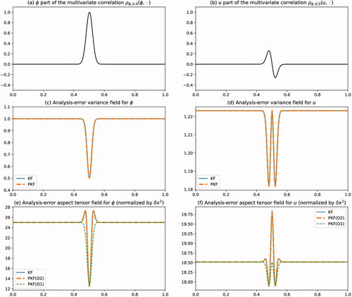
Now we focus on the analysis-error covariance matrix, explicitly computed from Eq. (1b)(1b) $${\mathbf{P}}^a=({\mathbf{I}}_n-\mathbf{KH}){\mathbf{P}}^f,$$(1b) for the KF, and whose the variance and the aspect tensor (a scalar field in this 1D situation) are shown in panels (c–d) for the variance and (e–f) for the aspect tensor. The assimilation of an observation of the field $\varphi$ implies a reduction of the forecast-error variance of $\varphi$ near the observation location, but also a reduction of the forecast-error variance of u, except at the observation point, while the field u is not observed. This is due to the multivariate covariance between the two fields $\varphi$ and u. An equivalent result is found for the aspect tensor for the field u that changes during the assimilation.

These diagnosis are now compared with the results provided by the PKF algorithms. This time, the computation of the PKF O2 and PKF O1 are done by using the multivariate correlation function of ${\mathbf{P}}^f,$ illustrated in panels (a, b). The analysis-error variance computed from the PKF are similar to the KF, the PKF O2 being nearly identical to the KF. For the analysis-error aspect tensor, the PKF O2 coincide with the KF while the PKF O1 only captures the reduction of the aspect tensor and not the overshoot. Note that, while the decrease of the analysis-error aspect tensor, from the background value for the observed variable $\varphi ,$ corresponds to what is well known, the increased for the variable u is new (as far as we know), and it is successfully captured by the PKF O2.

For this experiment, we conclude that the PKF applies in multivariate statistics, leading to the appropriate variance and aspect tensor fields $(V_{\varphi },V_u,{\mathit{s}}_{\varphi },{\mathit{s}}_u).$ To continue using the PKF by assimilating another observation, one need to update the correlation functions. However, since a covariance model of the kind of Eq. (26)(26) $$\begin{array}{c}{\mathbf{P}}^f=\left[\begin{array}{cc}\mathbf{I}& 0\\ \mathbf{D}& \mathbf{I}\end{array}\right]\left[\begin{array}{cc}{\mathbf{P}}_{\varphi }^u& 0\\ 0& {\mathbf{P}}_u^u\end{array}\right]\left[\begin{array}{cc}\mathbf{I}& {\mathbf{D}}^T\\ 0& \mathbf{I}\end{array}\right]=\\ \left[\begin{array}{cc}{\mathbf{P}}_{\varphi }^u& {\mathbf{P}}_{\varphi }^u{\mathbf{D}}^T\\ \mathbf{D}{\mathbf{P}}_{\varphi }^u& \mathbf{D}{\mathbf{P}}_{\varphi }^u{\mathbf{D}}^T+{\mathbf{P}}_u^u\end{array}\right]\end{array}$$(26) relies on the parameters ${\mathcal{P}}^u$ of the univariate unbalanced matrices ${\mathbf{P}}_{\varphi }^u$ and ${\mathbf{P}}_u^u,$ one has to determine ${\mathcal{P}}^u$ from $(V_{\varphi },V_u,{\mathit{s}}_{\varphi },{\mathit{s}}_u).$ Hence, an additional step is needed, and we detail how to proceed at a theoretical level.

5.2.2. Update of the parameters of the unbalanced univariate VLATcov matrices

The computation of ${\mathcal{P}}^u$ is performed from the sequential process described from Eq. (29), where the parameters of ${\mathbf{P}}_{\varphi }^u$ are first computed followed by those of ${\mathbf{P}}_u^u:$

Since ${\mathbf{P}}_{\varphi \varphi }={\mathbf{P}}_{\varphi }^u$ in Eq. (29a)(29a) $${\mathbf{P}}_{\varphi }^u={\mathbf{P}}_{\varphi \varphi },$$(29a) , the unbalanced parameters for $\varphi$ are directly obtained from $(V_{\varphi }^u,{\mathit{s}}_{\varphi }^u)=(V_{\varphi },{\mathit{s}}_{\varphi }).$

It remains to compute the unbalanced parameters of u, $(V_u^u,{\mathit{s}}_u^u),$ which can be deduced from the difference Eq. (29b)(29b) $${\mathbf{P}}_u^u={\mathbf{P}}_{uu}-\mathbf{D}{\mathbf{P}}_{\varphi }^u{\mathbf{D}}^T.$$(29b) that reads ${\mathbf{P}}_u^u={\mathbf{P}}_{uu}-\mathbf{D}{\mathbf{P}}_{\varphi \varphi }{\mathbf{D}}^T.$ As the covariance matrix $\mathbf{D}{\mathbf{P}}_{\varphi \varphi }{\mathbf{D}}^T$ is the covariance matrix of $\alpha {\partial }_x{\epsilon }_{\varphi },$ the variance, denoted by $V_{\alpha {\partial }_x\varphi }$ and it metric, denoted by ${\mathit{g}}_{\alpha {\partial }_x\varphi },$ are given by (30a) $$V_{\alpha {\partial }_x\varphi }={\alpha }^2\mathbb{E}\left[{({\partial }_x{\epsilon }_{\varphi })}^2\right],$$(30a) (30b) $${\mathit{g}}_{\alpha {\partial }_x\varphi }={\alpha }^2\mathbb{E}\left[{\left\{{\partial }_x\left(\frac{{\partial }_x{\epsilon }_{\varphi }}{\sqrt{V_{\alpha {\partial }_x\varphi }}}\right)\right\}}^2\right].$$(30b)

Using the definition of the metric field associated with ${\epsilon }_{\varphi }$ (see Eq. (6)(6) $$g_{ij}^f(\mathit{x})=\mathbb{E}\left[{\partial }_{x^i}\left(\frac{{\mathbf{\epsilon }}^f}{{\sigma }^f}\right){\partial }_{x^j}\left(\frac{{\mathbf{\epsilon }}^f}{{\sigma }^f}\right)\right](\mathit{x}),$$(6) ) the variance and the metric tensor of the balanced part reads (see e.g. Eq. (45)(B6) $$\begin{array}{l}{\mathit{g}}^a(\mathit{x})=\frac{V^f(\mathit{x})}{V^a(\mathit{x})}{\mathit{g}}^f(\mathit{x})+\\ \frac{1}{4V^f(\mathit{x})V^a(\mathit{x})}\left[\nabla V^f{(\nabla V^f)}^{\mathrm{T}}\right]-\\ \frac{1}{V^a(\mathit{x})}\frac{V^f({\mathit{x}}_l)}{V^f({\mathit{x}}_l)+V^o({\mathit{x}}_l)}\\ \left[\nabla ({\sigma }^f{\rho }_{{\mathit{x}}_l}^f){\left(\nabla ({\sigma }^f{\rho }_{{\mathit{x}}_l}^f)\right)}^{\mathrm{T}}\right](\mathit{x})-\\ \frac{1}{4{(V^a(\mathit{x}))}^2}\left[\nabla V^a{(\nabla V^a)}^{\mathrm{T}}\right](\mathit{x}).\end{array}$$(B6) in Appendix B) (31a) $$V_{\alpha {\partial }_x\varphi }={\alpha }^2\left(V_{\varphi }{\mathit{g}}_{\varphi }+\frac{1}{4V_{\varphi }}{({\partial }_x{V}_{\varphi })}^2\right),$$(31a) where ${\mathit{g}}_{\varphi }={({\mathit{s}}_{\varphi })}^{-1},$ and (31b) $${\mathit{g}}_{\alpha {\partial }_x\varphi }=\frac{{\alpha }^2}{V_{\alpha {\partial }_x\varphi }}\mathbb{E}\left[{({\partial }_x{}^2{\epsilon }_{\varphi })}^2\right]-\frac{{\alpha }^2}{4V_{\alpha {\partial }_x\varphi }^2}{\left({\partial }_x{V}_{\alpha {\partial }_x\varphi }\right)}^2.$$(31b)

Note that Eq. (31b)(31b) $${\mathit{g}}_{\alpha {\partial }_x\varphi }=\frac{{\alpha }^2}{V_{\alpha {\partial }_x\varphi }}\mathbb{E}\left[{({\partial }_x{}^2{\epsilon }_{\varphi })}^2\right]-\frac{{\alpha }^2}{4V_{\alpha {\partial }_x\varphi }^2}{\left({\partial }_x{V}_{\alpha {\partial }_x\varphi }\right)}^2.$$(31b) involves the high order statistic $\mathbb{E}\left[{({\partial }_x{}^2{\epsilon }_{\varphi })}^2\right]$ that is unknown in practice but for which a so-called Gaussian closure exists (Pannekoucke et al., 2018a). When no closure exists, a machine learning approach can be introduced to estimate a closure adapted to the application. To do so, automatic generation of neural networks can be useful (Pannekoucke and Fablet, 2020). Then, the statistics of the unbalance part of u reads (32a) $$V_u^u=V_u-V_{\alpha {\partial }_x\varphi },$$(32a) (32b) $${\mathit{g}}_u^u=\frac{1}{V_u^u}\left(V_u{\mathit{g}}_u-V_{\alpha {\partial }_x\varphi }{\mathit{g}}_{\alpha {\partial }_x\varphi }\right),$$(32b) where Eq. (32b)(32b) $${\mathit{g}}_u^u=\frac{1}{V_u^u}\left(V_u{\mathit{g}}_u-V_{\alpha {\partial }_x\varphi }{\mathit{g}}_{\alpha {\partial }_x\varphi }\right),$$(32b) is obtained from a local homogeneous assumption (Pannekoucke et al., 2020, see the proof in their Appendix B), with ${\mathit{g}}_u={\mathit{s}}_u^{-1};$ leading to ${\mathit{s}}_u^u={({\mathit{g}}_u^u)}^{-1}.$

5.2.3. Discussion on the PKF in the multivariate setting

We have shown that it is possible to compute the parameters ${\mathcal{P}}^u$ from the results of the PKF algorithms 1 and 2, leading to a PKF formulation for the multivariate parametric model Eq. (26)(26) $$\begin{array}{c}{\mathbf{P}}^f=\left[\begin{array}{cc}\mathbf{I}& 0\\ \mathbf{D}& \mathbf{I}\end{array}\right]\left[\begin{array}{cc}{\mathbf{P}}_{\varphi }^u& 0\\ 0& {\mathbf{P}}_u^u\end{array}\right]\left[\begin{array}{cc}\mathbf{I}& {\mathbf{D}}^T\\ 0& \mathbf{I}\end{array}\right]=\\ \left[\begin{array}{cc}{\mathbf{P}}_{\varphi }^u& {\mathbf{P}}_{\varphi }^u{\mathbf{D}}^T\\ \mathbf{D}{\mathbf{P}}_{\varphi }^u& \mathbf{D}{\mathbf{P}}_{\varphi }^u{\mathbf{D}}^T+{\mathbf{P}}_u^u\end{array}\right]\end{array}$$(26) : in algorithms 1 and 2, an additional step is added after the update of the variance and metric tensor fields of the multivariate statistics to update the unbalanced variance and metric tensors fields.

So, the design of a PKF implementation for the analysis in the multivariate framework that relies on VLATcov models, is possible, but needs to be adapted for the particular multivariate model used.

Note that, the theoretical expressions of the update of the unbalanced parameters, that have been introduced here, offer a new insight into multivariate analysis. However, particular attention should be given to the case when closure issues occur, and in practice other alternatives to analytical closures can be investigated e.g. the estimation of the unbalanced parameters leveraged on machine learning techniques. This kind of strategy can increase the cost of the PKF. Thus, the interest of the PKF depends on the cost of using other alternatives to compute the analysis-error covariance matrix, so it depends on the application we consider.

As a final comment, observe that the batch strategy can still be used in the multivariate situation, as far as the observational-error correlation can be neglected.

6. Conclusions

The parametric Kalman filter (PKF) is a new nonlinear Kalman-like filter where the error covariance matrices are approximated using a parametric covariance model (Pannekoucke et al. 2016, 2018a, P16). We considered the parametric covariance model based on a diffusion equation used in NWP, for which the set of parameters is reduced to the variance and the local diffusion tensor fields. The diffusion covariance model is an example of covariance model parametrized by the variance field and the local anisotropic tensors (VLATcov). Another example of VLATcov model has been considered from Theorem 1 of Paciorek and Schervish (2004), and in particular the heterogeneous Gaussian VLATcov which appears here as a surrogate for the diffusion VLATcov. In this contribution, the PKF analysis step for VLATcov model has been detailed, which extends the original 1D version of the PKF of P16 to dimension larger than one and to a wider family of covariance models. Two consistent implementations of the PKF for the VLATcov has been presented for the heterogeneous Gaussian VLATcov model: the PKF O2 and its local homogeneous version, the PKF O1.

This study constitutes a theoretical contribution to the realm of data assimilation, featuring analytical results for the analysis uncertainty and illustrating these results using numerical experiments. The validation of the PKF was conducted in a 2D test-bed. A univariate numerical framework with anisotropic forecast error correlation functions was introduced to show the ability of the PKF analysis step to reproduce the KF statistics. Then an experiment of several assimilations cycles has shown the ability of the PKF to reproduce the KF statistics which have been computed from an ensemble estimation. In particular, the PKF O1 has shown to be a more robust implementation than the PKF O2. Thus, the PKF O1 may be preferred in applications since it appears as a compromise between precision and robustness. The multivariate situation has been explored at a theoretical level. This contribution provides a new insight into univariate and multivariate assimilations e.g. the expression of how the metric tensor updates in 2D/3D domains; and draws some ways to adapt the univariate PKF toward the multivariate case.

The strength of the PKF is that it applies to continuous fields, making its numerical cost less sensitive to the dimension of discretization than for methods based on matrix computation. In the experiment conducted here, the numerical cost of the PKF analysis step is well below the numerical cost of an ensemble Kalman filter (EnKF), which makes the PKF an interesting alternative to the EnKF, especially for real-time applications, e.g. now-casting of high impact weather situations as encountered in chemical transport models for chemical accidents and volcanic ash prediction. Moreover, the single observation experiment applies to both univariate and multivariate settings, bringing the PKF closer to real-world applications. However, an additional step has to be introduced in multivariate statistics that depends on the multivariate parametric model used for the covariance.

But there is still work to be done for using the PKF analysis in NWP. In its current form, the PKF does not take into account correlation in observation errors. Note that the sequential assimilation, used in the PKF, can apply when observational errors are correlated by considering a sub-sampled observational network (as it is often done in NWP data assimilation). Furthermore, the modelling of multivariate error covariance is still a challenge: the balance operator modelling of the variational assimilation appears as an interesting way to start. While the PKF forecast step has been already discussed for linear and nonlinear dynamics in univariate statistics (Pannekoucke et al., 2016, 2018a), the multivariate case remains to be developed. The promising results obtained here, also suggest considering a data-driven strategy to learn the update of the covariance parameters, taking advantage of machine learning for the analysis step as well as for the forecast step: convolutional neural networks would be adapted for this (Pannekoucke and Fablet, 2020).

As other applications, the PKF analysis could replace the often-used optimal interpolation, providing an update of the uncertainty during the sequential assimilation. Observation targeting could also benefit of the low-cost computation of the analysis error statistics given by the PKF. Note that the 2D/3D univariate formulation developed here can be used without further developments in some important applications e.g. in air quality where the operational assimilation often updates chemical concentrations independently each others; or to accelerate the assimilation for the prediction of the consequences of industrial accidents. To this end, the illustration of the PKF over several assimilation cycles shows the potential of the PKF to perform an approximation for the KF.

Note that, more generally, the PKF not only leads to practical implementations of the KF equations, but it also provides theoretical tools for understanding the data assimilation process e.g. the exploration of the model-error covariance due to the numerical discretization (Pannekoucke et al., 2020).

Acknowledgments

We would like thank Isabelle Mirouze, Marc Bocquet and Richard Ménard, for interesting discussions and comments on the manuscript. We would like to thank the two anonymous referees for their fruitful comments which have contribute to improve the manuscript. This work was supported by the French national program LEFE/INSU (Étude du filtre de KAlman PAramétrique, KAPA).

Disclosure statement

No potential conflict of interest was reported by the author.

Additional information

Funding

This research has been supported by the LEFE INSU (KAPA grant).

Appendix A:

derivation of the local metric tensor from error statistics

Here, a differentiable random field $\epsilon$ with zero mean is considered (i.e. $\mathbb{E}(\epsilon )=0$).

The two-point correlation is defined as (A1) $$\rho (\mathit{x},\mathit{x}+\delta \mathit{x})=\mathbb{E}\left[\left(\frac{\epsilon }{\sigma }\right)(\mathit{x})\left(\frac{\epsilon }{\sigma }\right)(\mathit{x}+\delta \mathit{x})\right],$$(A1) where $\sigma (\mathit{x})=\sqrt{\mathbb{E}[\epsilon {(x)}^2]}$ denotes the standard-deviation field associated with $\epsilon .$ From the Taylor expansion, (A2) $$\begin{array}{l}\left(\frac{\epsilon }{\sigma }\right)(\mathit{x}+\delta \mathit{x})=\left(\frac{\epsilon }{\sigma }\right)(\mathit{x})+\\ \sum _i\delta x^i{\partial }_{x^i}\left(\frac{\epsilon }{\sigma }\right)(\mathit{x})+\\ \frac{1}{2}\sum _{i,j}\delta x^i\delta x^j{\partial }_{x^i{x}^j}^2\left(\frac{\epsilon }{\sigma }\right)(\mathit{x})+o(|\left|\delta \mathit{x}\right|{|}^2),\end{array}$$(A2) where the little-o $f(x)\underset{a}{=}o(g(x))$ means that $\underset{x\to a}{\lim }\frac{f(x)}{g(x)}=0,$ and the correlation Eq. (A1)(A1) $$\rho (\mathit{x},\mathit{x}+\delta \mathit{x})=\mathbb{E}\left[\left(\frac{\epsilon }{\sigma }\right)(\mathit{x})\left(\frac{\epsilon }{\sigma }\right)(\mathit{x}+\delta \mathit{x})\right],$$(A1) can be written as (A3) $$\begin{array}{l}\rho (\mathit{x},\mathit{x}+\delta \mathit{x})=\mathbb{E}\left[\left(\frac{\epsilon }{\sigma }\right)(\mathit{x})\left(\frac{\epsilon }{\sigma }\right)(\mathit{x})\right]+\\ \sum _i\delta x^i\mathbb{E}\left[\left(\frac{\epsilon }{\sigma }\right)(\mathit{x}){\partial }_{x^i}\left(\frac{\epsilon }{\sigma }\right)(\mathit{x})\right]+\\ \sum _{i,j}\frac{1}{2}\delta x^i\delta x^j\mathbb{E}\left[\left(\frac{\epsilon }{\sigma }\right)(\mathit{x}){\partial }_{x^i{x}^j}^2\left(\frac{\epsilon }{\sigma }\right)(\mathit{x})\right]+o(|\left|\delta \mathit{x}\right|{|}^2).\end{array}$$(A3)

Because the variance field $\mathbb{E}\left[\left(\frac{\epsilon }{\sigma }\right)(\mathit{x})\left(\frac{\epsilon }{\sigma }\right)(\mathit{x})\right]$ is homogeneously equal to one, it follows that (A4) $${\partial }_{x^i}\mathbb{E}\left[\left(\frac{\epsilon }{\sigma }\right)(\mathit{x})\left(\frac{\epsilon }{\sigma }\right)(\mathit{x})\right]=0.$$(A4)

Since the spatial derivative ${\partial }_{x^i}$ commutes with the $\mathbb{E},$ then (A5) $$\begin{array}{l}{\partial }_{x^i}\mathbb{E}\left[\left(\frac{\epsilon }{\sigma }\right)(\mathit{x})\left(\frac{\epsilon }{\sigma }\right)(\mathit{x})\right]=\\ \mathbb{E}\left[{\partial }_{x^i}\left\{\left(\frac{\epsilon }{\sigma }\right)(\mathit{x})\left(\frac{\epsilon }{\sigma }\right)(\mathit{x})\right\}\right]=\\ 2\mathbb{E}\left[\left(\frac{\epsilon }{\sigma }\right)(\mathit{x}){\partial }_{x^i}\left(\frac{\epsilon }{\sigma }\right)(\mathit{x})\right],\end{array}$$(A5) from which it can be deduced that (A6) $$\mathbb{E}\left[\left(\frac{\epsilon }{\sigma }\right)(\mathit{x}){\partial }_{x^i}\left(\frac{\epsilon }{\sigma }\right)(\mathit{x})\right]=0.$$(A6)

Similarly, (A7) $$\begin{array}{c}\mathbb{E}\left[\left(\frac{\epsilon }{\sigma }\right)(\mathit{x}){\partial }_{x^i}\left(\frac{\epsilon }{\sigma }\right)(\mathit{x})\right]=0.\\ -\mathbb{E}\left[\left({\partial }_{x^i}\frac{\epsilon }{\sigma }\right)(\mathit{x}){\partial }_{x^j}\left(\frac{\epsilon }{\sigma }\right)(\mathit{x})\right].\end{array}$$(A7)

Therefore, the correlation can be written as (A8) $$\begin{array}{l}\rho (\mathit{x},\mathit{x}+\delta \mathit{x})=\\ 1-\sum _{i,j}\frac{1}{2}\delta x^i\delta x^j\mathbb{E}\left[{\partial }_{x^i}\left(\frac{\epsilon }{\sigma }\right)(\mathit{x}){\partial }_{x^j}\left(\frac{\epsilon }{\sigma }\right)(\mathit{x})\right]+\\ o(|\left|\delta \mathit{x}\right|{|}^2).\end{array}$$(A8)

Because the local metric tensor $\mathit{g}(\mathit{x})$ is defined via the Taylor expansion, (A9) $$\rho (\mathit{x},\mathit{x}+\delta \mathit{x})=1-\frac{1}{2}\left|\right|\delta \mathit{x}|{|}_{\mathit{g}(\mathit{x})}^2+o(\left|\right|\delta \mathit{x}|{|}^2).$$(A9)

Identifying the local metric tensor in the last two expressions of the correlation leads to the identity (A10) $${\left[\mathit{g}\right]}_{ij}(\mathit{x})=\mathbb{E}\left[{\partial }_{x^i}\left(\frac{\epsilon }{\sigma }\right)(\mathit{x}){\partial }_{x^j}\left(\frac{\epsilon }{\sigma }\right)(\mathit{x})\right].$$(A10)

Appendix B:

PKF analysis step for a single observation assimilation

By introducing the true state and the error fields ${\mathcal{X}}^a={\mathcal{X}}^t+{\mathit{\epsilon }}^a,$ ${\mathcal{X}}^f={\mathcal{X}}^t+{\mathit{\epsilon }}^f$ and ${\mathcal{Y}}^o({\mathit{x}}_l)={\mathcal{X}}^t({\mathit{x}}_l)+{\mathit{\epsilon }}^o({\mathit{x}}_l),$ the analysis equation, Eq. (13a)(13a) $$\begin{array}{l}{\mathcal{X}}^a(\mathit{x})={\mathcal{X}}^f(\mathit{x})+{\sigma }^f(\mathit{x}){\rho }_{{\mathit{x}}_l}^f(\mathit{x})\\ \frac{{\sigma }^f({\mathit{x}}_l)}{V^f({\mathit{x}}_l)+V^o({\mathit{x}}_l)}({\mathcal{Y}}^o({\mathit{x}}_l)-{\mathcal{X}}^f({\mathit{x}}_l)),\\ \end{array}$$(13a) , becomes (B1) $$\begin{array}{c}{\mathit{\epsilon }}^a(\mathit{x})={\mathit{\epsilon }}^f(\mathit{x})+{\sigma }^f(\mathit{x}){\rho }_{{\mathit{x}}_l}^f(\mathit{x})\\ \frac{{\sigma }^f({\mathit{x}}_l)}{V^f({\mathit{x}}_l)+V^o({\mathit{x}}_l)}\left({\mathit{\epsilon }}^o({\mathit{x}}_l)-{\mathit{\epsilon }}^f({\mathit{x}}_l)\right).\end{array}$$(B1)

Then, it is straightforward to compute the analysis error variance field $V^a(\mathit{x})=\mathbb{E}({\mathit{\epsilon }}^a{(\mathit{x})}^2),$ which can be written as (B2) $$V^a(\mathit{x})=V^f(\mathit{x})\left(1-{[{\rho }_{{\mathit{x}}_l}^f(\mathit{x})]}^2\frac{V^f({\mathit{x}}_l)}{V^f({\mathit{x}}_l)+V^o({\mathit{x}}_l)}\right).$$(B2)

This is a classic result of optimal interpolation (Daley, 1991, pp. 146–147).

From the definition of the local metric tensor, Eq. (6)(6) $$g_{ij}^f(\mathit{x})=\mathbb{E}\left[{\partial }_{x^i}\left(\frac{{\mathbf{\epsilon }}^f}{{\sigma }^f}\right){\partial }_{x^j}\left(\frac{{\mathbf{\epsilon }}^f}{{\sigma }^f}\right)\right](\mathit{x}),$$(6) , the analysis error local metric tensor, expanded in terms of the variance, is written (B3) $$\begin{array}{l}{\mathit{g}}^a(\mathit{x})=\frac{1}{V^a(\mathit{x})}\mathbb{E}\left[\nabla {\epsilon }^a{(\nabla {\epsilon }^a)}^{\mathrm{T}}\right](\mathit{x})-\\ \frac{1}{4{(V^a(\mathit{x}))}^2}\left[\nabla V^a{(\nabla V^a)}^{\mathrm{T}}\right](\mathit{x}).\end{array}$$(B3)

As the observation and the forecast errors are assumed uncorrelated, so that $\mathbb{E}({\mathit{\epsilon }}^f(\mathit{x}){\mathit{\epsilon }}^o({\mathit{x}}_l))=0$ (since $\mathbb{E}[{\mathit{\epsilon }}^f]=0$ and $\mathbb{E}[{\mathit{\epsilon }}^o]=0$), and using the fact that $\mathbb{E}({\mathit{\epsilon }}^f(\mathit{x}){\mathit{\epsilon }}^f({\mathit{x}}_l))={\sigma }^f(\mathit{x}){\sigma }^f({\mathit{x}}_l){\rho }^f({\mathit{x}}_l,\mathit{x})$ is the covariance relative to the position ${\mathit{x}}_l,$ the gradient of Eq. (B1)(B1) $$\begin{array}{c}{\mathit{\epsilon }}^a(\mathit{x})={\mathit{\epsilon }}^f(\mathit{x})+{\sigma }^f(\mathit{x}){\rho }_{{\mathit{x}}_l}^f(\mathit{x})\\ \frac{{\sigma }^f({\mathit{x}}_l)}{V^f({\mathit{x}}_l)+V^o({\mathit{x}}_l)}\left({\mathit{\epsilon }}^o({\mathit{x}}_l)-{\mathit{\epsilon }}^f({\mathit{x}}_l)\right).\end{array}$$(B1) yields (B4) $$\begin{array}{c}\mathbb{E}\left[\nabla {\epsilon }^a{(\nabla {\epsilon }^a)}^{\mathrm{T}}\right](\mathit{x})=\mathbb{E}\left[\nabla {\epsilon }^f{(\nabla {\epsilon }^f)}^{\mathrm{T}}\right](\mathit{x})-\\ \frac{V^f({\mathit{x}}_l)}{V^f({\mathit{x}}_l)+V^o({\mathit{x}}_l)}\left[\nabla ({\sigma }^f{\rho }_{{\mathit{x}}_l}^f){\left(\nabla ({\sigma }^f{\rho }_{{\mathit{x}}_l}^f)\right)}^{\mathrm{T}}\right](\mathit{x}).\end{array}$$(B4)

Using the definition of the forecast error metric tensor, (B5) $$\begin{array}{c}{\mathit{g}}^f(\mathit{x})=\frac{1}{V^f(\mathit{x})}\mathbb{E}\left[\nabla {\epsilon }^f{(\nabla {\epsilon }^f)}^{\mathrm{T}}\right](\mathit{x})-\\ \frac{1}{4{(V^f(\mathit{x}))}^2}\left[\nabla V^f{(\nabla V^f)}^{\mathrm{T}}\right](\mathit{x}),\end{array}$$(B5) the analysis error metric tensor can be written in arbitrary dimensions as (B6) $$\begin{array}{l}{\mathit{g}}^a(\mathit{x})=\frac{V^f(\mathit{x})}{V^a(\mathit{x})}{\mathit{g}}^f(\mathit{x})+\\ \frac{1}{4V^f(\mathit{x})V^a(\mathit{x})}\left[\nabla V^f{(\nabla V^f)}^{\mathrm{T}}\right]-\\ \frac{1}{V^a(\mathit{x})}\frac{V^f({\mathit{x}}_l)}{V^f({\mathit{x}}_l)+V^o({\mathit{x}}_l)}\\ \left[\nabla ({\sigma }^f{\rho }_{{\mathit{x}}_l}^f){\left(\nabla ({\sigma }^f{\rho }_{{\mathit{x}}_l}^f)\right)}^{\mathrm{T}}\right](\mathit{x})-\\ \frac{1}{4{(V^a(\mathit{x}))}^2}\left[\nabla V^a{(\nabla V^a)}^{\mathrm{T}}\right](\mathit{x}).\end{array}$$(B6)

References

- Belo Pereira, M. and Berre, L. 2006. The use of an ensemble approach to study the background error covariances in a global NWP model. Mon. Weather Rev. 134, 2466–2489. doi:https://doi.org/10.1175/MWR3189.1
- Berre, L. O., Pannekoucke, G., Desroziers, S., Stefanescu, S. E., Chapnik, B. and Raynaud, L. 2007. A variational assimilation ensemble and the spatial filtering of its error covariances: increase of sample size by local spatial averaging. In ECMWF Workshop on Flow-Dependent Aspects of Data Assimilation, 11–13 June 2007. Reading, UK, pp. 151–168.
- Bocquet, M., Raanes, P. and Hannart, A. 2015. Expanding the validity of the ensemble Kalman filter without the intrinsic need for inflation. Nonlin. Processes Geophys. 22, 645–662. doi:https://doi.org/10.5194/npg-22-645-2015
- Bonavita, M., Isaksen, L. and Hólm, E. 2012. On the use of eda background-error variances in the ecmwf 4d-var. Q. J. R. Meteorol. Soc. 138, 1540–1559. doi:https://doi.org/10.1002/qj.1899
- Bormann, N., Saarinen, S., Kelly, G. and Thépaut, J.-N. 2003. The spatial structure of observation errors in atmospheric motion vectors from geostationary satellite data. Mon. Wea. Rev. 131, 706–718. doi:https://doi.org/10.1175/1520-0493(2003)131<0706:TSSOOE>2.0.CO;2
- Bouttier, F. 1994. A dynamical estimation of error covariances in an assimilation system. Mon. Wea. Rev. 122, 2376–2390. doi:https://doi.org/10.1175/1520-0493(1994)122<2376:ADEOFE>2.0.CO;2
- Cohn, S. 1993. Dynamics of short-term univariate forecast error covariances. Mon. Wea. Rev. 121, 3123–3149. doi:https://doi.org/10.1175/1520-0493(1993)121<3123:DOSTUF>2.0.CO;2
- Coman, A., Foret, G., Beekmann, M., Eremenko, M., Dufour, G. et al. 2012. Assimilation of IASI partial tropospheric columns with an ensemble Kalman filter over Europe. Atmos. Chem. Phys. 12, 2513–2532. doi:https://doi.org/10.5194/acp-12-2513-2012
- Daley, R. 1991. : Atmospheric Data Analysis. New York, USA: Cambridge University Press, 472pp.
- Derber, J. and Bouttier, F. 1999. A reformulation of the background error covariance in the ecmwf global data assimilation system. Tellus A 51, 195–221. doi:https://doi.org/10.3402/tellusa.v51i2.12316
- Evensen, G. 2009. : Data Assimilation: The Ensemble Kalman Filter. Springer-Verlag Berlin Heidelberg: Springer, 332 pp.
- Fisher, M. 2003. Background error covariance modelling. In Proceedings of ECMWF Seminar on Recent Developments in Data Assimilation for Atmosphere and Ocean, Reading, UK, pp. 45–63.
- Gaspari, G. and Cohn, S. 1999. Construction of correlation functions in two and three dimensions. QJ. Royal Met. Soc. 125, 723–757. doi:https://doi.org/10.1002/qj.49712555417
- Houtekamer, P. L. and Mitchell, H. 1998. Data assimilation using an ensemble Kalman filter technique. Mon. Wea. Rev. 126, 796–811. doi:https://doi.org/10.1175/1520-0493(1998)126<0796:DAUAEK>2.0.CO;2
- Houtekamer, P. and Mitchell, H. 2001. A sequential ensemble Kalman filter for atmospheric data assimilation. Mon. Wea. Rev. 129, 123–137. doi:https://doi.org/10.1175/1520-0493(2001)129<0123:ASEKFF>2.0.CO;2
- Houtekamer, P., Mitchell, H. L., Pellerin, G., Buehner, M., Charron, M., et al. 2005. Atmospheric data assimilation with an ensemble Kalman filter: results with real observations. Mon. Wea. Rev. 133, 604–620. doi:https://doi.org/10.1175/MWR-2864.1
- Hristopulos, D. 2002. New anisotropic covariance models and estimation of anisotropic parameters based on the covariance tensor identity. Stoch. Environ. Res. Risk Assess. 16, 43–62. doi:https://doi.org/10.1007/s00477-001-0084-y
- Hunt, B. R., Kostelich, E. J. and Szunyogh, I. 2007. Efficient data assimilation for spatiotemporal chaos: a local ensemble transform Kalman filter. Physica D 230, 112–126. doi:https://doi.org/10.1016/j.physd.2006.11.008
- Kalman, R. E. 1960. A new approach to linear filtering and prediction problems. J. Basic Eng. 82, 35–45. doi:https://doi.org/10.1115/1.3662552
- Massart, S., Piacentini, A. and Pannekoucke, O. 2012. Importance of using ensemble estimated background error covariances for the quality of atmospheric ozone analyses. Qjr. Meteorol. Soc. 138, 889–905. doi:https://doi.org/10.1002/qj.971
- Ménard, R. and L.-P. Chang, 2000. Assimilation of stratospheric chemical tracer observations using a Kalman filter. Part II: chi-2-validated results and analysis of variance and correlation dynamics. Mon. Wea. Rev. 128, 2672–2686. AOSCTO⟩2.0.CO;2. doi:https://doi.org/10.1175/1520-0493(2000)128<2672:AOSCTO>2.0.CO;2
- Ménard, R., Cohn, S., Chang, L.-P. and Lyster, P. M. 2000. Assimilation of stratospheric chemical tracer observations using a Kalman filter. Part I: Formulation. Mon. Wea. Rev. 128, 2654–2671. doi:https://doi.org/10.1175/1520-0493(2000)128<2654:AOSCTO>2.0.CO;2
- Mirouze, I. and Weaver, A. T. 2010. Representation of correlation functions in variational assimilation using an implicit diffusion operator. Q. J. R. Meteorol. Soc. 136, 1421–1443. doi:https://doi.org/10.1002/qj.643
- Paciorek, C. and Schervish, M. 2004. Nonstationary covariance functions for gaussian process regression. Adv. Neural Inf. Process. Syst. 16, 273–280.
- Pannekoucke, O. and Massart, S. 2008. Estimation of the local diffusion tensor and normalization for heterogeneous correlation modelling using a diffusion equation. Qjr. Meteorol. Soc. 134, 1425–1438. doi:https://doi.org/10.1002/qj.288
- Pannekoucke, O. and Fablet, R. 2020. PDE-NetGen 1.0: from symbolic partial differential equation (PDE) representations of physical processes to trainable neural network representations. Geosci. Model Dev. 13, 3373–3382. doi:https://doi.org/10.5194/gmd-13-3373-2020
- Pannekoucke, O., Emili, E. and Thual, O. 2014. Modeling of local length-scale dynamics and isotropizing deformations. Qjr. Meteorol. Soc. 140, 1387–1398. doi:https://doi.org/10.1002/qj.2204
- Pannekoucke, O., Ricci, S., Barthelemy, S., Ménard, R. and Thual, O. 2016. Parametric Kalman filter for chemical transport model. Tellus 68, 31547. doi:https://doi.org/10.3402/tellusa.v68.31547
- Pannekoucke, O., Bocquet, M. and Ménard, R. 2018a. Parametric covariance dynamics for the nonlinear diffusive burgers’ equation. Nonlinear Process. Geophys. 2018, 1–21.. https://www.nonlin-processes-geophys-discuss.net/npg-2018-10/.
- Pannekoucke, O., Ricci, S., Barthelemy, S., Ménard, R. and Thual, O. 2018b. Parametric Kalman filter for chemical transport models - corrigendum. Tellus A: Dynamic Meteorology and Oceanography 70, 1–2.
- Pannekoucke, O., Ménard, R., Aabaribaoune, M. E. and Plu, M. 2020. A methodology to obtain model-error covariances due to the discretization scheme from the parametric Kalman filter perspective. Nonlinear Process. Geophys. 28, 1–22.
- Purser, R., Wu, W.-S., Parrish, D. and Roberts, N. 2003. Numerical aspects of the application of recursive filters to variational statistical analysis. Part II: Spatially inhomogeneous and anisotropic general covariances. Mon. Weather Rev. 131, 1536–1548. doi:https://doi.org/10.1175//2543.1
- Sakov, P. and Sandery, P. A. 2015. Comparison of EnOI and EnKF regional ocean reanalysis systems. Ocean Modell. 89, 45–60. doi:https://doi.org/10.1016/j.ocemod.2015.02.003
- Warming, R. and Hyett, B. 1974. The modified equation approach to the stability and accuracy analysis of finite-difference methods. Comput. Phys. 14, 159–179. doi:https://doi.org/10.1016/0021-9991(74)90011-4
- Weaver, A. and Courtier, P. 2001. Correlation modelling on the sphere using a generalized diffusion equation (Tech. Memo. ECMWF, num. 306). Q. J. R. Meteorol. Soc. 127, 1815–1846. doi:https://doi.org/10.1002/qj.49712757518
- Weaver, A. T. and Mirouze, I. 2013. On the diffusion equation and its application to isotropic and anisotropic correlation modelling in variational assimilation. Qjr. Meteorol. Soc. 139, 242–260. doi:https://doi.org/10.1002/qj.1955
- Weaver, A., Deltel, C., Machu, E., Ricci, S. and Daget, N. 2005. A multivariate balance operator for variational ocean data assimilation. Q J. R Meteorol. Soc. 131, 3605–3625. doi:https://doi.org/10.1256/qj.05.119
- Wu, W.-S., Purser, R. J. and Parrish, D. F. 2002. Three-dimensional variational analysis with spatially inhomogeneous covariances. Mon. Wea. Rev. 130, 2905–2916. doi:https://doi.org/10.1175/1520-0493(2002)130<2905:TDVAWS>2.0.CO;2