Environmental control of land-atmosphere CO₂ fluxes from temperate ecosystems: a statistical approach based on homogenized time series from five land-use types

Abstract

We assembled homogenized long-term time series, up to 19 years, of measurements of net ecosystem exchange of CO₂ (NEE) and its partitioning between gross primary production (GPP) and respiration (R_eco) for five different ecosystems representing the main plant functional types (PFTs) in France. Part of these data was analyzed to determine the influence of the main environmental variables on carbon fluxes between temperate ecosystems and the atmosphere, and to investigate the temporal patterns of their variations. A multi-temporal statistical analysis of the time series was conducted using random forest (RF) and wavelet coherence approaches. The RF analysis showed that, in all ecosystems, the incident solar radiation was highly correlated with GPP and that GPP was better correlated with the temporal variations of NEE than R_eco. The air temperature was the second most important driver in ecosystems with seasonal foliage, i.e., deciduous forest, cropland and grassland; whereas variables related to air or soil drought were prominent in evergreen forest sites. The environmental control on CO₂ fluxes was tighter at high frequency suggesting an increased resilience to environmental variations at longer time spans. The spectral analysis performed on three of the five sites selected revealed contrasting temporal patterns of the cross-coherence between CO₂ fluxes and climate variables among ecosystems; these were related to the respective PFT, management and soil conditions. In all PFTs, the power spectrum of GPP was well correlated with NEE and clearly different from R_eco. The spectral correlation analysis showed that the canopy phenology and disturbance regime condition the spectral correlation patterns of GPP and R_eco with the soil moisture and atmospheric vapour deficit.

Keywords:

• Net CO2 ecosystem exchange
• Ecosystem respiration
• Gross primary production
• spectral analysis
• random forest analysis

1. Introduction

The analysis of time series of eddy-covariance (EC) data, as in-situ measurements of the net atmospheric CO₂ exchange (NEE) reveals that their temporal variability is a ubiquitous phenomenon which may help investigations of the sensitivity of biogeochemical processes to the environment at the ecosystem scale. Over the past decade, numerous studies have focused on the interannual variability (IAV) of NEE and its environmental drivers at global scale (Jung et al. 2017; Liu et al. 2018; Fu et al. 2019). Studies were conducted for different ecosystems (Delpierre et al. 2012; Shao et al. 2016; Baldocchi et al. 2018; Fu et al., 2018) and individual sites (Wohlfahrt et al. 2008; Marcolla et al. 2011; Aubinet et al. 2018). Synthesis studies have reported significant spatial variability in NEE among ecosystem types (Baldocchi 2008; Niu et al. 2017; Baldocchi et al. 2018), as well as large temporal variability within sites.

The IAV of NEE at the ecosystem scale has been primarily linked to meteorological drivers (including extreme events) such as temperature, precipitation, and radiation, etc. Plant phenology is an additional control acting through, e.g., the length of the growing season, and the timing of leaf onset and shedding. Evidence exists that these drivers are significant contributors to the temporal variability of NEE. Subtler changes in the ecosystem structure due to natural and anthropogenic disturbances (e.g., stand/cropland/grassland management) or delayed physiological response to climate, and edaphic conditions, are also likely causes. Indeed, the variations in temperature, precipitation and incident solar radiation have been reported as the most important climate factors controlling variability in the NEE of different ecosystems (Jung et al. 2017), while less attention has been paid to climate interactions with phenology and physiology (i.e., period and amplitude of the growing season) (Delpierre et al. 2009). The direct and indirect controlling factors of the NEE IAV differ among the ecosystem types, with distinctive differences between forests and non-forests, evergreen needleleaf forests (ENF) and deciduous broadleaf forests (DBF), and between grasslands (GRA) and croplands (CRO) (Shao et al. 2016).

The response of the gross primary productivity (GPP) and ecosystem respiration (R_eco) to physical and biological drivers controls the variability of NEE at different time scales, from seconds to years (Stoy et al. 2009). Long-term observations are necessary to capture such effects (Chu et al. 2017). Most recent studies indicate that IAV of NEE is most often associated with variations in GPP (Ciais et al. 2005; Stoy et al. 2009; Ahlström et al. 2015; Novick et al. 2016). In a synthesis study, Shao et al. (2016) found that the maximum photosynthetic rate was the most important factor for the IAV in GPP, which was mainly induced by the variation in vapour pressure deficit (D). For R_eco, the most important drivers were GPP and the reference respiratory rate. The relative sensitivity of photosynthesis and respiration to environmental factors shows that GPP is more sensitive to drought stress than R_eco in most ecosystems. This phenomenon was especially the case in Mediterranean climates, which experience large variability in the amount of rainfall during the growing season (Pereira et al. 2007; Allard et al. 2008).

Several methodologies have been used in the literature to explore carbon-flux/environment interactions. Common approaches are based on the statistical analysis between carbon cycle components and environmental variables applied on measured data. Among them, look-up tables are used for gap-filling (Falge et al., 2001; Reichstein et al. 2005). A number of numerical, analytical or predictive approaches, either detailed or simplified, have been proposed, which are grouped into the so-called Machine Learning approach (ML). Detailed or simplified ML can be applied to predict carbon fluxes based on environmental parameters. The approach has proved good at demonstrating the nonlinear relationship between ecosystem-based carbon fluxes and environmental variables based on EC measurements (Papale and Valentini 2003). These authors have demonstrated the potential of artificial neural networks in the study of carbon flux dynamics in European forest ecosystems, for gap-filling and spatializing carbon fluxes (Dou et al. 2015; Papale et al. 2015). In predictive studies of soil CO₂ fluxes, or carbon and energy fluxes, ML based on the Random Forest approach (RF) (Dou et al. 2018) or regression splines (Tramontana et al. 2016) have been successfully used. The RF approach is highly flexible and can perform two types of data analysis: regression and classification. In our study specifically, we used the regression mode as our variables are continuous. RF is of particular interest because it determines the most important environmental parameters controlling the variations in carbon fluxes at different time scales. Spectral analysis is also an appropriate technique to investigate the control of fluxes in the time-frequency domain, which is therefore complementary to the RF approach. Previous studies used Fourier transform or cross-correlation approaches, (Baldocchi et al. 2001; Stoy et al. 2005, 2009; Vargas et al. 2010a). More recently the alternative technique of wavelet analysis has emerged (Vargas et al. 2010b, 2011; Fares et al. 2013). The latter is particularly relevant for investigating the spectral properties of biometeorological variables that exhibit non-stationary features (Katul et al. 2001) and for partitioning the drivers of their temporal variability along the frequency domain. In that sense, the scalogram — plot of a signal spectrum or a two-signal cross-spectrum as a function of time and frequency — can be more useful than the spectrogram for analyzing real-world signals that are typically non-stationary. Trends in means and/or variability are typical features of such signals, but changing modes of variability could also be present. Scalograms are the dedicated tools for detecting the latter. They also have the advantage of better time localization for short-duration/high-frequency events, and better frequency localization for low-frequency, longer-duration events.

Comparing the interaction between carbon fluxes and environmental parameters among different ecosystems requires concurrent time series of turbulent data obtained with a common methodology and standardized post-processing treatments. Thus far, this requirement has not yet been satisfactorily met for the various methodologies used either when measuring turbulent variables or for processing the data obtained. Moreover, concurrent time series of flux and meteorological data extending beyond 10 years were not available until recently. The present study is built upon time series of data from different types of ecosystems representative of the French network of stations contributing to the European ICOS Research Infrastructure. Among them, three historical stations were launched during the Euroflux project in 1997 and two during the subsequent CarboEuroflux project in 2000 and 2002. The data analyzed represent the carbon flux components, the Net Ecosystem Exchange, Gross Primary Production and total ecosystem Respiration. They cover the five main temperate plant functional types along time series extending from 9 to 13 years. The values of the three flux components were calculated from raw data using a common methodology thus eliminating artificial discrepancies between sites.

Our analysis investigates the respective influence of the drivers of NEE, GPP and R_eco. It uses a Random Forest analysis performed along a range of discrete frequencies and a spectral analysis for the determination of cross-coherence between CO₂ fluxes and their environmental drivers across the frequency domain.

2. Material and methods

2.1. Site descriptions

Five sites from the pre-ICOS network were selected for the analysis, as representative of plant functional types in France:

• A temperate Deciduous Broadleaf Forest (DBF): hereafter referred to as Barbeau

• A temperate Evergreen Needleleaf Forest (ENF): Le Bray

• A Mediterranean Evergreen Broadleaf Forest (EBF): Puechabon

• A temperate/continental extensive Grassland (GRA): Laqueuille

• A temperate Cropland (CRO): Auradé

The site characteristics are summarized in Fig. 1 and Table 1. Additional information is provided in the supplementary material (S1, Table S1).

Fig. 1. Location of sites in France.

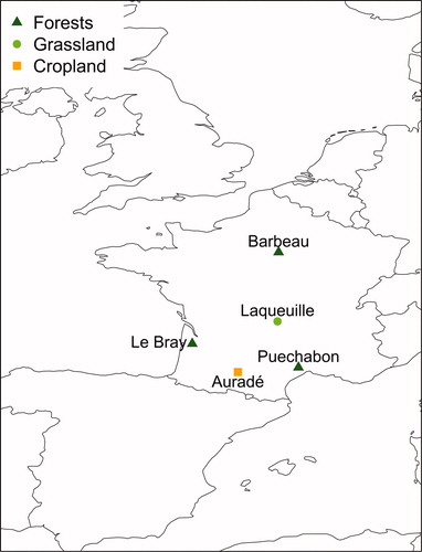
Table 1. Experimental sites characteristics.

Sites	Pre-ICOS names	Coordinates	Ecosystem characteritics	Environment	Averages	References
Puechabon	FR-Pue	43°44’29”N, 03°35’45”E, 270 m elevation	PFT: Evergreen Broadleaf Forest (EBF) Species: Holm oak (Quercus ilex) Understorey : Buxus sempervirens, Phyllirea latifolia, Pistacia terebinthus and Juniperus oxycedrus LAI: 2.7 ± 0.3 m^2 m^-2 (overstorey) Management: Coppice Last cut : 1942	Climate : Mediterranean Soil: Shallow bedrock : 75% in the top 0–50 cm 90% below Stone-free fine fraction of the top-soil: 38.8% clay 35.2% silt 26% sand. Water holding capacity: 140 mm.	Period: 1984–2016 Temperature: 13.3 °C Precipitation: 923 mm	Allard et al. (2008); Cabon et al. (2018)
Barbeau	FR-Fon	48°28’37’’N, 02°46’56’’E, 89 m elevation	PFT: Deciduous Broadleaf Forest (DBF) Species : Dominant : sessile oak (Quercus Petraea, (Matt.) Liebl. 160 yrs old) Sublayer : Hornbeam (Carpinus betulus L., 60-70 yrs old) LAI : 5.3 m^2 m^-2 (2005–2016 average) Management : coppice	Climate: Mild oceanic temperate Soil: Oligo-mull humus, Gleyic luvisol: 30% clay 37% silt 33% sand Millstone bedrock at 0.9 m depth Water holding capacity: ∼ 170 mm.	Period: 1980–2010 Temperature: 11.2 °C Precipitation: 677 mm	Delpierre et al. (2009); Delpierre et al. (2016)
Le Bray	FR-LBr	44°43’02”N, 00°46’10”W, 62 m elevation	PFT: Evergreen Needleleaf Forest (ENF) Species:  Mature maritime pine (Pinus Pinaster Aït.) Understorey : Molench coerulea (L.) Moench LAI : 2.6 to 3.1 m^2 m^-2 (overstorey) Management: Seeding: 1970 Thinning: 1990, 1995, 2002, 2005	Climate: Oceanic temperate Soil: Humic sandstone : 2% clay 98% sand Impermeable layer of Ferruginous cement in the B horizon at 0.9 m depth (alios). Water holding capacity: ∼120 mm.	Period: 1987–2008 Temperature: 12.5 °C Precipitation: 932 mm	Loustau and Granier (1993); Granier and Loustau (1994); Jarosz et al. (2008); Ogée et al. (2003)
Auradé	FR-Aur	43°32’59’’N, 01°06’22’’E, 245 m elevation	PFT: Cropland (CRO) Species: Rotation of rapeseed, winter wheat and sunflower (see Table S1) PAI : 0 to 5 m^2 m^-2 (2005–2014) Management : No irrigation (see Table S1)	Climate: Temperate Soil: 32.3% clay 47.1% silt 20.6% sand,	Period: 2004–2014 Temperature: 13 °C Precipitation: 680 mm	Béziat et al. (2009); Etchanchu et al. (2017)
Laqueuille	FR-Laq	45°38’34’’N, 02°44’02’’E, 1040 m elevation	PFT: Extensive grassland (GRA) Species: Grass LAI : 1.5 m^2 m^-2 (average) Management: Extensive no fertilization and grazed continuously by heifers from May to October with a lowLivestock Unit (LSU) of 0.6 SLU ha^-1 yr^-1	Climate: Temperate/continental Soil: Andosol developed on basaltic rocks. Loamy texture content (18% with a C:N ratio of 10.5)	Period: 2004–2014 Temperature: 7.9 °C Precipitation: 1000 mm	Klumpp et al. (2011)

2.2. Meteorological data and flux measurements

The time series of in-situ measurements analyzed by the RF or wavelet approaches are summarized in Table 2. Among them, we used the incident solar radiation (S_d), the air temperature (T_air), the precipitations (P), the wind speed (u), the vapour pressure deficit (D) computed from the air temperature and the relative humidity, and the soil water content (θ). The relative extractable water (θ_EW) was computed from the volumetric soil water content (θ) normalized by the water holding capacity estimated from the difference between the water content at field capacity and at wilting point (Granier et al. 1999), previously quantified for these specific sites. When θ was not available or when the data series contained too many gaps, a site-specific model for the corresponding site was used to gap-fill θ_EW (Granier et al. 1999; Mouillot et al. 2001; Loustau et al. 2005; Vuichard et al. 2007; Cabon et al. 2018, supplementary material § S2).

Table 2. Setup at each site. T_air stands for air temperature at measurement height (in °C), RH for relative humidity (in %), S_d for incoming shortwave radiation (in W m⁻²), u for wind speed (in m s⁻¹), P for precipitation (in mm), θ for soil water content (in mm).

Sites Measurement height	Data processed	Variables		Instruments	Statistical analysis period (^1 or ^2)
Puechabon 12.2m	2001–2014	Meteorological variables :	Tair/RH : Sd : u : P : θ :	MP100 (Rotronic Inst. Corp., Huntington, NY, USA) SKS1110 (Skye Inst. Ltd, Powys, UK) A100R (Campbell Scientific Inc, Logan, UT, USA) ARG100 (Environmental Measurements Ltd., Sunderland, UK) TDR Trase (Soil Moisture Equipment Corp., Santa Barbara, CA, USA)	2001–2014^1 2006–2011^2
		Micrometeorological variables :	3D u : CO2/H2O :	GILL-R3 (Gill Instruments Ltd, Lymington, Hampshire, UK) LI-6262 (Li-Cor Inc., Lincoln, NE, USA)
Barbeau 37m	2005–2018	Meteorological variables :	Tair/RH : Sd : u : P :	HMP155A (Vaisala, Helsinki, Finland) CMP22 (Kipp & Zonen, Delft, NL) WindSonic (Gill Instruments Ltd) 3029/2 (Précis Mécanique SAS, Bezons, France)	2005–2018^1 2006–2011^2
		Micrometeorological variables :	3D Ws : 2005-2018 2012-2018 CO2/H2O : 2005-2018 2012-2018	GILL-R3-50 (Gill Instruments Ltd) GILL-HS-50 (Gill Instruments Ltd) LI-7500 (Li-Cor Inc., Lincoln, NE, USA) LI-7200 (Li-Cor Inc., Lincoln, NE, USA)
Le Bray 41m	2000–2008	Meteorological variables :	Tair/RH : Sd : u : P : θ :	HMP45 (Vaisala, Helsinki, Finland) CE180 (Cimel Electronique, Paris, France) 05103 (Young, Traverse city, MI, USA) ARG100 (Campbell Scientific Inc, Logan, UT, USA) TDR Trase (Soil Moisture Equipment Corp., Santa Barbara, CA, USA)	2000–2008^1
		Micrometeorological variables :	3D u : CO2/H2O :	GILL-R2 (Gill Instruments) LI-7500 (Li-Cor Inc., Lincoln, NE, US)
Auradé 2m	2005–2014	Meteorological variables :	Tair/RH : Sd : u : P : θ :	HMP35A (Vaisala, Helsinki, Finland) CNR1/CNR4 (Kipp & Zonen, Delft, NL) 05103 (Young, Traverse city, MI, USA) ARG100 (Environmental Measurements Ltd., Sunderland, UK) CS616 (Campbell Scientific Inc, Logan, UT, USA)	2005–2014^1 2006–2011^2
		Micrometeorological variables :	3D u : CO2/H2O :	CSAT3 (Campbell Scientific Inc, Logan, UT, USA) LI-7500 (Li-Cor Inc., Lincoln, NE, USA)
Laqueuille 2m	2004–2013	Meteorological variables :	Tair/RH : Sd : u : P : θ :	HMP155A (Vaisala, Helsinki, Finland) SKS1110 (Skye Inst. Ltd, Powys, UK) 05103 (Young, Traverse city, MI, USA) 52202 (Young, Traverse city, MI, USA) CS616 (Campbell Scientific Inc, Logan, UT, USA)	2004–2013^1
		Micrometeorological variables :	3D u : CO2/H2O :	GILL-R3 (Gill Instruments Ltd) LI-7500 (Li-Cor Inc., Lincoln, NE, USA)

The net ecosystem exchange (NEE) was determined using the eddy-covariance methodology which combines measurement at 20 Hz of the 3-D wind speed and surrogate temperature using a sonic anemometer, and with the molar fractions of CO₂/H₂O using an infrared gas analyzer (see Table 2 for sensor references at each site).

2.3. Eddy-covariance data processing

2.3.1. Flux computation

Half-hourly eddy-covariance fluxes from the five selected sites were calculated using EddyPro® (www.licor.com/eddypro). Standardized processing was applied for all the sites. i) Axis rotation of the wind vector was performed using the planar fit methodology (Wilczak et al. 2001) for Barbeau, Puechabon, Le Bray, Laqueuille and the double rotation for Auradé because of the fast growth rate of the vegetation. The block-average method was used to extract turbulent fluctuations from time series (Gash and Culf 1996). Time lags between vertical wind speed and the variable of interest were determined for each averaging period by an automatic time lag optimization. ii) Low frequency spectral corrections were applied according to the analytic method described by Moncrieff et al. (2005). High frequency spectral corrections were applied depending on the setup: the fully analytic method of Moncrieff et al. (1997) was adopted for the open-path systems (LI-7500, Auradé, Laqueuille, Barbeau), which includes a correction for sensor separation effects; an in-situ spectral correction method (Fratini et al. 2012) was used for the closed-path analyzers (LI-6262, Puechabon and Le Bray) as a suitable method to describe attenuation along the intake tube. For the closed-path analyzers, a correction was also applied to account for sonic anemometer and analyzer separation according to Horst and Lenschow (2009). For the open-path LI-7500 analyzers, the WPL correction (Webb et al. 1980) and the self-heating correction were also applied (Burba et al. 2008). iii) As a QA/QC test of the final fluxes, we used the standard flags (0-1-2) defined by Mauder and Foken (2004) and data with a flag = 2 were discarded. Remaining flux data were also filtered using statistical tests on the raw data (Vickers and Mahrt 1997); these included: despiking, absolute limit determination, amplitude resolution, drop out, skewness and kurtosis tests, and discontinuities. Finally, we tested for insufficient atmospheric turbulence with a friction velocity (u_* threshold being determined for each site (Reichstein et al. 2005).

2.3.2. Partitioning and gap-filling

Incident solar radiation (S_d), air temperature, T_air and vapour pressure deficit (D) were gap-filled using the marginal distribution method (Reichstein et al. 2005). To compare CO₂ fluxes computed over different integrated time scales from the different sites, we filled gaps in the half-hourly flux time series using the gap-filling tool and the nighttime partitioning method from Reichstein et al. (2005), developed in an R package (Wutzler et al. 2018). An exception was made for Barbeau for which the 2013 NEE long gap of the LI-7500 was gap-filled with the flux computed from the LI-7200 deployed in parallel with the LI-7500 since 2012 (Delpierre N., pers. comm).

2.4. Statistical analyses

2.4.1. Random forest analyses

A random forest (RF) machine-learning algorithm (Breiman 2001) was used to identify how the environmental controls affect the variability of NEE, GPP and R_eco in the long term. The RF is a non-parametric statistical estimation technique based on the use of decision trees and multiple regressions. A detailed explanation of the algorithm is given by Breiman (2001). Each of the decision trees that form an RF are built from bootstrap samples of the original dataset (i.e., training data). For each tree, the data that are not included in the bootstrap samples are named Out-Of-Bag (OOB) samples (i.e., test data). The training data is randomly chosen for the splitting rule at each node. Each tree is then fully grown or until each node is pure. The trees are not pruned.

Using the OOB samples, the RF algorithm produces a robust and informative statistic able to provide the importance of an explanatory variable X for predicting the variable of interest Y (McInerney and Nieuwenhuis 2009). This importance of explanatory variables, X, over the response variables, Y, is calculated in terms of percentage increase of the mean squared error (%IncMSE) if the variable X in the model is replaced with a random one (Eq. 1). (1) $$\mathrm{MSE}=\frac{\sum _{i=1}^n{\left(Y-\widehat{Y}\right)}^2}{n}$$(1) where: Y stands for the observed variable, $\widehat{Y}=f(X)$ for the predictive variable, n the number of observations.

More precisely, an explanatory variable, X, is considered important if by “breaking” the link between X and Y, the prediction error increases. To break this link, Breiman (2001) suggested randomly permuting the predictor variable, X, in the OOB samples. The importance corresponds to the mean increase in the prediction error on the tree ensemble. Therefore, if we randomly permute an explanatory variable that does not gain us anything in prediction, then predictions will not change much and we will only see small changes in MSE. On the other hand, the important variables will significantly change the predictions if randomly permuted, so we will see more significant changes in MSE. The higher the difference is, the more important is the explanatory variable.

The package ‘randomForest’ (Version 4.6-14, Liaw and Wiener 2018) available in R was used for these multiple regression analyses and is presented in the supplementary material (S3). The analysis was conducted first to compare five plant functional types (PFTs) at the half-hourly time-step. Secondly, we performed the analyses at weekly, monthly and seasonal scales for only two sites, those presenting contrasting results at the half-hourly time-step. Among the data presented in section 2.2, the data used for the RF analyses were S_d, T_air, P, u, D, θ_EW, and carbon dioxide concentration (CO₂). To make the graphs easier to read at the aggregated time scales, we aggregated radiative parameters into an ‘Energy’ variable (S_d + T_air) and an Index of Stress relative to the air or soil water deficit constraint defined by ‘IStress’ (θ_EW+ D). In order to cross-compare the %IncMSE computed at each site and for each flux, we present this %IncMSE as a relative value of the total percentage (%Imp).

Missing environmental values are omitted in the analysis. Indeed, to make sure that the final results were not biased by the partitioning and gap-filling method that is based on a relationship between hourly R_eco and T_air, and GPP and S_d, we performed the analyses using only measured NEE (qc = 0), nighttime R_eco (S_d < 20 W m⁻²) and daytime GPP (S_d > 20 W m⁻²) when it was directly estimated from NEE minus R_eco.

2.4.2. Wavelet coherence analyses

Local and global wavelet power spectra were computed using the Morlet wavelet transform (Morlet et al. 1982). Morlet proposed the use of a window with a size that depends on the frequency analyzed, with a fixed number of oscillations. The analyzed functions are precisely the Morlet wavelets that allow us to:

1. Observe the high frequencies with a high temporal resolution and therefore to provide accurate information on the locations of brief phenomena.

2. Observe the low frequencies over a sufficient period of analysis to account for slow phenomena.

The Morlet wavelet transform of a time series (x_t) is defined as the convolution of the series with a set of “wavelet daughters” generated by the mother wavelet $\mathrm{\Psi },\mathrm{ }$ by translation in time by τ and scaling by s (Eq. 2) (Rösch and Schmidbauer 2018). The position of the particular daughter wavelet in the time domain is determined by the localizing time parameter τ being shifted by a time increment δt. δt is therefore the time resolution, i.e. the sampling resolution in the time domain, and 1/δt represents the number of observations per time unit. The choice of the set of scales s determines the wavelet coverage of the series in the frequency domain. This scale value is a fractional power of 2, a ‘voice’ in an ‘octave’ with 1/δj determining the number of voices per octave. δj corresponds to the frequency resolution, i.e. the sampling resolution in the frequency domain, and therefore, 1/δj refers to the number of suboctaves, i.e., voices per octave. (2) $$W_x\left(\mathrm{\tau },s\right)=\mathrm{ }\sum _t{x}_t\frac{1}{\sqrt{s}}{\mathrm{\Psi }}^{\mathrm{*}}\left(\frac{t-\mathrm{\tau }}{s}\right)$$(2)

They also defined the wavelet power spectrum or time-frequency (or time-period) wavelet energy density: (3) $$P_x\left(\mathrm{\tau },s\right)=\mathrm{ }\frac{1}{s}\mathrm{ }\times {\left|W_X\left(\mathrm{\tau },s\right)\right|}^2$$(3) which actually corresponds to the square of the local amplitude of the periodic component of the time series.

Following the approach of Torrence and Webster (1999), the wavelet coherence between two time series ($x_t$) and ($y_t$) was computed as: (4) $$\mathit{Coherence}=\mathrm{ }\frac{{\left|\mathrm{S}\times W_{xy}\right|}^2}{\mathrm{S}\times P_x\mathrm{ }\times \mathrm{ }\mathrm{S}{\times P}_y}$$(4)

The notion of wavelet coherence requires smoothing of both the cross-wavelet spectrum and the normalizing individual wavelet power spectra, which is indicated by ‘S’ smoothing operator and is defined as S(W(τ, s)) = S_scale (S_time(W(τ, s))). S_time represents smoothing in time and S_scale is smoothing along the wavelet scale axis. $W_{xy}$ is the cross-wavelet transform (Eq. 5), defined as the product of the wavelet transform of $x$ and the complex conjugate of the wavelet transform of $y$ (Torrence and Compo 1998): (5) $$W_{x\mathrm{y}}=\mathrm{ }\frac{1}{s}\mathrm{ }\times \mathrm{ }{W}_x\left(\mathrm{\tau },s\right)\times \mathrm{ }{W_y}^{\mathrm{*}}\left(\mathrm{\tau },s\right)$$(5) where “*” denotes the complex conjugate.

Squared spectral coherence estimates, as described by Eq. 4(4) $$\mathit{Coherence}=\mathrm{ }\frac{{\left|\mathrm{S}\times W_{xy}\right|}^2}{\mathrm{S}\times P_x\mathrm{ }\times \mathrm{ }\mathrm{S}{\times P}_y}$$(4) , express the degree of linear association between the phases and amplitudes of the two data records within each normalized non-overlapping frequency band. These estimates show the proportion of common variance within each frequency band shared by two variables. Eq. (4) is the analogue with the notion of Fourier coherence and the coefficient of determination in statistics. It may actually be regarded as such, which means that a coherence value of zero signifies that the two time series are unrelated, whereas a coherence value of unity indicates the two time series are linearly related at the given frequency and time. Finally, through this cross-wavelet analysis, we can study the two series synchronization in terms of the instantaneous or local phase advance of any periodic component of ($x_t$) with respect to the correspondent component of ($y_t$), the so-called phase difference of $x$ over $y$ at each localizing time origin and scale. (6) $$\Delta \phi \left(\mathrm{\tau },s\right)=\mathrm{ }\mathit{Arg}{\left(W_{xy}\right(\mathrm{\tau },s\left)\right)}^{}$$(6)

Eq. 6(6) $$\Delta \phi \left(\mathrm{\tau },s\right)=\mathrm{ }\mathit{Arg}{\left(W_{xy}\right(\mathrm{\tau },s\left)\right)}^{}$$(6) equals the difference of individual phases, Δφ = φ_x−φ_y, when converted to an angle in the interval] −π, π].

The package ‘WaveletComp’ (Version 1.1, Rösch and Schmidbauer (2018)) available in R was used for these coherence analyses. The parameters used in the analysis and the scalogram reading guidelines are provided in the supplementary documentation (Supplementary material: § S3.2, S3.3 and Table S2, Fig. S2). All the results are presented as image plots of both the individual wavelet power spectrum (and average) and cross-wavelet coherence, in the time-period domain for the period 2006–2011. This period was selected as a common period for the three selected sites and with the lowest gap-filled data percentage. Since, among the five sites considered, our Random Forest analysis allowed us to identify three main patterns and our power and wavelet results are shown for three sites selected out of the five original sites: a forest with permanent foliage, Puechabon (similar to Le Bray), a forest with seasonal foliage, Barbeau, and the crop site, Auradé (similar to Laqueuille). The cross-coherence analyses focused on the most important meteorological parameters extracted from the Random Forest analysis, i.e. θ_EW and D. They comprise both the main potential constraints on carbon fluxes (Novick et al. 2016) and exhibit a stronger and less predictive temporal variability than S_d and T_air across sites. In addition, spectral analysis of the cross-coherence of these two variables with carbon flux components from 30 minutes to 6 years has rarely been performed.

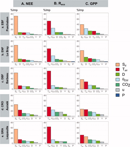
Fig. 2. RF analysis results: importance of environmental variables explaining the variability of carbon fluxes (A. NEE, B. GPP and C. R_eco) at a half-hourly time-step at five ecosystem stations. Standard deviation on the mean of %imp of each environmental variable, computed from a bootstrap analysis (n = 100), were voluntarily omitted in the graph as they presented values lower than 0.1% in each case (See Supplementary material S3.1).

3. Results

Firstly, we are presenting the analyses of the role and importance of environmental drivers in determining the variability of carbon fluxes for the five sites selected over the whole period of measurement provided in Table 2 at each site. This phase does not need any specific description of the environmental conditions as it is based on the RF approach mixing all environmental conditions. Thereafter we are showing the investigations on the temporal correlation between time series for three of the five sites selected by identifying periodicities and quantifying phase differences between series for a range of temporal scales. The analyses were performed on a 6-year period (2006–2011) for which environmental and fluxes patterns are described.

3.1. Random forest analysis

At half-hourly resolution, the percentage of variance explained by the RF model showed values between 65% and 90% (Table 3) and was higher by between 4% and 30% for NEE and R_eco as compared with GPP. For all five sites, S_d was the most important factor in explaining NEE and GPP, accounting for more than 45% of the half-hourly variability; whereas T_air was responsible for most of the variability of R_eco (>70%), followed by θ_EW (Fig. 2). The atmospheric concentration of CO₂ appeared third in the list of factors explaining the variance of GPP, R_eco and NEE for poor mixing conditions (R_eco) and canopies with lowest roughness (grassland at Laqueuille and crops at Auradé). The precipitation contribution was negligible.

Table 3. Input parameters optimization and results of the RF approach in terms of percentage of variance explained from the half-hourly (five sites), daily, monthly and seasonal (two sites selected) time scales. « ndata » corresponds to the number of data in the time-step considered; « mtry » stands for the number of explanatory variables to randomly sample as candidates at each split and « ntrees » for the number of trees in the RF analysis.

See Supplementary material (§ S3.1) for further information.

Sites	Years	Flux	ndata	mtry	ntrees	% Var Explained	MSE
Half-hourly :
Puechabon	2000–2014	Reco	40400	6	400	88.55	0.16
		GPP	59527	4	400	73.27	5.92
		NEE	99927	2	400	85.84	3.17
Le Bray	2000–2008	Reco	20128	6	400	86.04	0.43
		GPP	36176	2	400	67.91	16.4
		NEE	56305	2	400	79.27	11.4
Barbeau	2005–2018	Reco	51049	6	400	88.89	0.37
		GPP	66170	3	400	82.87	21.9
		NEE	117220	3	400	86.58	12.8
Auradé	2004–2014	Reco	23475	5	400	74.12	0.69
		GPP	36094	4	400	64.9	36.1
		NEE	59570	4	400	72.33	17.5
Laqueuille	2003–2013	Reco	19391	5	400	90.05	0.62
		GPP	25832	4	400	69.25	18.6
		NEE	45223	2	400	72.8	13.0
Daily :
Puechabon	2000–2014	Reco	3340	4	400	60.4	0.61
		GPP	4311	3	400	62.88	5.13
		NEE	4456	2	400	51.43	4.63
Auradé	2004–2014	Reco	2421	5	400	40.56	1.64
		GPP	2721	4	400	43.97	38.3
		NEE	2842	3	400	53.56	12.2
Monthly :
Puechabon	2000–2014	Reco	166	7	400	58.3	0.53
		GPP	167	4	400	53.29	3.45
		NEE	167	5	400	58.38	1.00
Auradé	2004-2014	Reco	114	5	400	46.36	1.21
		GPP	114	7	400	63.17	22.3
		NEE	114	5	400	71.04	4.63
Seasonnally :
Puechabon	2000–2014	Reco	56	3	400	41.22	0.40
		GPP	56	7	400	20.99	4.10
		NEE	56	3	400	65.72	0.46
Auradé	2004–2014	Reco	40	5	400	37.36	1.07
		GPP	40	3	400	51.27	25.5
		NEE	40	4	400	54.05	6.14

Three main results were revealed by this analysis at half-hourly time-step:

• Globally, the four most important variables extracted were S_d, T_air, D, and θ_EW (Fig. 2).

• The pattern of RF for NEE was roughly similar to the GPP’s with S_d being the largest contributor and either θ_EW, D or T_air second.

• R_eco was instead systematically dominated by the T_air contribution with θ_EW ranked second contributor.

3.1.1. PFT comparison

The main difference between PFTs came from the variance profiles of GPP and NEE. For those PFTs with strong LAI dynamics during the year, i.e., Barbeau, Laqueuille, Auradé, T_air appears as the second most important variable after the incident radiation. The θ_EW or D only appeared as third or fourth-most important contributors, wind speed and precipitation being last. Conversely, for evergreen PFTs Puechabon (holm oak) and Le Bray (maritime pine), the θ_EW and D came second in the variance profiles of GPP and NEE, θ_EW being the most important parameter at Puechabon and D at Le Bray.

3.1.2. Analysis across integration times

Across time scales, the GPP-NEE similarity was conserved from the 30-minute time scale to the seasonal at the cropland site, but the precipitation overtook the stress contribution at the season scale (Fig. 3B). At Puechabon, the GPP profile was changed and the stress index became the main contributor to GPP at monthly and seasonal scales (Fig. 3A).

Fig. 3. RF analysis results: importance of environmental variables explaining the carbon flux variabilities for Puechabon (A) and Auradé (B) at different time scales. Standard deviation on the mean of %imp of each environmental variable, computed from a bootstrap analysis (n = 1000), were voluntarily omitted in the graph as they presented values lower than 1.5% for each case (§ S3.1).

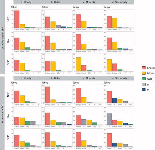
According to the integration time considered, the variables selected did capture a variable fraction of the carbon flux variability in the evergreen broadleaf at the Puechabon site and the cropland at Auradé, from 21% (the seasonal variance of GPP at Puechabon) to 89% (the half-hourly R_eco at Puechabon) (Table 3). In the EBF, the variance contribution profile was maintained at the different scales, with the dominance of S_d (more than 50% for the different scales) for NEE. However, the constraint index, ‘IStress’, contributed gradually to the variability reaching almost 50% of the seasonal variance (Fig. 3). R_eco patterns did not significantly change except for the season for which D and θ_EW equally contributed to the variability (35%) and the precipitation contribution reached 4% against 0.3% at the hourly scale. Finally, the GPP variability was mainly affected by the θ_EW from daily to seasonal scale, that became the most important variable across increasing time scales. Including D, these two potential constraints contributed to 64% and 56% at monthly and seasonal scales, respectively.

In the cropland, as regards NEE and GPP, S_d and Istress were still dominant along the different scales (sum >50%). However, precipitation became as important as Istress at seasonal scale. For R_eco, we also observed an increasing importance of wind speed especially at seasonal scale (>50%). The difference in performance between the two PFTs, EBF and crops (CRO), decreased at longer time scales.

We focused the next analyses on three sites that presented contrasting results in the RF analyses (Barbeau, Puechabon and Auradé), and for a common period 2006–2011 with the lowest amount of gap-filled data.

3.2. Environmental conditions and carbon flux time series over the period 2006–2011

3.2.1. Environmental conditions

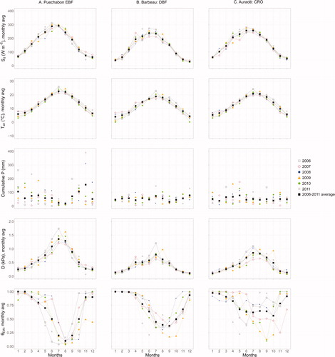
The 2006–2011 period was characterized by contrasting environmental conditions that are depicted for three sites, Barbeau, Auradé and Puechabon, in Fig. 4 and Supplementary material: section S4 and Table S3. The average annual temperatures (See Table S3) were slightly higher than the long-term average (Table 1). The highest monthly average temperature was recorded either in July or August, with values of 19.7 °C, 21.7 °C and 23.3 °C for Barbeau, Auradé and Puechabon, respectively. The warmest year was 2011, followed by 2006 and 2009. The year 2010 was coldest, despite a warm July, in part due to two months in winter and autumn being colder than the long-term average. Solar radiation during the spring varied strongly between years, with periods such as May 2011 presenting a significant increase in S_d at the three sites, compared to the other years. This increase is consistent with the low rainfalls recorded at the same time. Similarly, November 2011 had the lowest solar radiation at Puechabon; consistent with the highest amount of rainfall. Further comments are provided in Supplementary material S4.

Fig. 4. 2006–2011 monthly time series of environmental variables (S_d, T_air, Cumulative P, u and D) for the three sites selected in the wavelet analyses.

3.2.2. Carbon fluxes: 2006–2011

Using the sign convention that a flux from the vegetation to the atmosphere is positive, the annual balance of carbon (NEE) in the evergreen broadleaf forest (EBF) ranged from −381 g C m⁻²yr⁻¹ (2007) to −136 g C m⁻²yr⁻¹ (2006) and from −579 g C m⁻²yr⁻¹ (2007) to −425 g C m⁻²yr⁻¹ (2006) in the deciduous broadleaf forest (DBF) with a smaller year-to-year variability than at the other sites during the studied period (Fig. 5, Table S3). At Auradé, the winter wheat rotations were a carbon sink with carbon sequestration between −166 g C m⁻²yr⁻¹ and −11 g C m⁻²yr⁻¹, whereas rapeseed and sunflower rotations were sources of carbon (+12 and +176 g C m⁻²yr⁻¹ respectively).

Fig. 5. 2006–2011 monthly time series of carbon fluxes (NEE, GPP, and R_eco), for the three sites selected in the wavelet analyses.

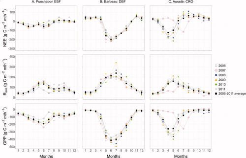
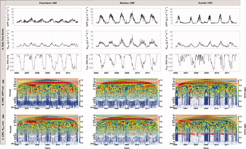
Fig. 6. Wavelet Power Spectra (WPS) of environmental variables (scalograms) and corresponding profile of the average wavelet power (curves) at three sites (Puechabon, Barbeau and Auradé).

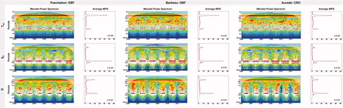
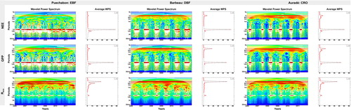
Fig. 7. Wavelet Power Spectra (WPS) of ecosystem carbon fluxes (scalograms) and corresponding profile of the average wavelet power (curves) at three sites (Puechabon, Barbeau and Auradé).

The temperate DBF site presented the highest gross primary production (GPP) between 1829 g C m⁻²yr⁻¹ (2006) and 2162 g C m⁻²yr⁻¹ (2011) with no significant differences between years, considering the uncertainty on the measurements (about ±10%, Baldocchi et al. 2018). The Mediterranean EBF GPP ranged from 986 g C m⁻²yr⁻¹ (2006) to 1475 g C m⁻²yr⁻¹ (2007) and the crop had the lowest annual values of GPP ranging from 642 g C m⁻²yr⁻¹ (sunflower rotation in 2007) to 1239 g C m⁻²yr⁻¹ (winter wheat, 2008). The temperate DBF site also presented the highest R_eco between 1404 g C m⁻²yr⁻¹ (2006) and 1616 g C m⁻²yr⁻¹ (2011). In the Mediterranean EBF, R_eco ranged from 847 g C m⁻²yr⁻¹ (2006) to 1091 g C m⁻²yr⁻¹ (2007) with no significant difference between years. The annual R_eco ranged from 742 g C m⁻²yr⁻¹ (for the sunflower, 2007) and 1125 g C m⁻²yr⁻¹ (for the winter wheat, 2010). The annual peak in both GPP and R_eco was observed in May/June in the cropland (except for the sunflower, in July) in June for the EBF and July for the DBF.

3.3. Power and cross-coherence spectra of CO₂ fluxes and climate variables at multi-temporal scales

The power and wavelet analyses were performed at three sites representing different plant functional types (PFTs) and for which the RF analysis showed contrasting patterns (Puechabon, Barbeau and Auradé). In what follows, the cross-correlation of ecosystem fluxes with θ_EW and D was more specifically investigated as these two variables represent a potential stress on carbon fluxes with a stronger and less predictive temporal variability than S_d and T_air across sites. In addition, spectral analysis of the cross-coherence of these two variables with carbon fluxes from 30 minutes to 6 years has rarely been performed. For all scalograms, red colours indicates high power whereas blue colours indicates low power.

3.3.1. Individual power spectra of climate variables (Fig. 6)

Despite the range of climates covered, the power spectra of meteorological variables and their temporal variations from 2006 to 2011 were similar among the three sites. For each variable, the average wavelet power showed two major peaks at 1-year and 1-day bands. The water vapour deficit and soil moisture variables showed, however, the distinct features documented below.

• The water vapour deficit (D) spectrum reflected both the low frequency pattern shown by temperature and the high frequency behaviour of S_d. It exhibited high power at intermediate scales, from 8-day to 3-month periods, only during the summer season. Plausible explanations of the discrepancy between the temperature and water vapour saturation deficit at high frequency may be the frequent zeroing of D values during nighttime and the non-linear relationship between temperature and air water vapour saturation which both amplify the daily D variation for a given step change in temperature.

• At all sites, the relative extractable soil moisture content, θ_EW, is characterized by narrow bands of high power extending from 1-year down to 2-week periods. It showed little variation at periods shorter than a month. Different patterns can be seen, which appear to depend on the soil thickness. For soil deeper than 1 m, a 12-month periodicity is observed continuously for θ_EW irrespective of plant functional type (EBF or DBF). Power peaks (red colour) are observed at higher frequency only after heavy precipitation at the end of the summer/autumn in 09–10/2006, 11/2008, and autumn 2011 for Puechabon (EBF) and 10/2008, 08/2010 and 08/2011 for Barbeau (DBF). The rainstorms in late autumn have even induced locally high power peaks of θ_EW at intermediate frequency bands (periods < 1 month). No such patterns are observed during summer. We assume this is because high frequency precipitation events in summer only marginally affect the soil water volumetric content because of a dilution effect and the interception of precipitation by the vegetation canopy that is proportionally higher for lighter rainfall episodes and during summer. For the shallowest soil (Auradé), the power at the year period is intermittent whereas clear pulse dynamics are observed at high frequency (1 per day). Indeed, due to the shallower soil in the cropland (Auradé), the response of θ and θ_EW to precipitation events at higher frequencies is strong, as seen by the spikes at 3-hour to 6-month periodicities attributed to wetting-drying cycles. This was observed for all years, except 2008 when the cropland soil was close to saturation throughout the year and the θ_EW remained above 0.7 from June to September.

3.3.2. Individual power spectra of CO₂ fluxes (Fig. 7)

Over the 6-year period considered, the effect of the annual cycle of leaf formation and leaf fall is evident in the measured CO₂ fluxes. This is particularly clear at Barbeau deciduous broadleaf forest, meanwhile the fluxes from the cropland were controlled by the farming operations between the sowing and the harvest date. The Puechabon evergreen Mediterranean broadleaf forest had no distinctive periodic pattern.

NEE and GPP. At high frequencies and in accordance with the RF analysis, the wavelet decomposition of NEE and GPP were strikingly similar, suggesting that processes driving temporal variations of GPP were also controlling NEE, more than temporal variations of R_eco. Power spectra of NEE and GPP had significant high power at the 1-day period and a secondary small peak at 0.5 day during the growing season. Hence, the high frequency peaks were limited to spring-summer for the DBF and cropland, but covered the entire year in the EBF type. There was one exception however during winter 2008–2009 in the cropland where a secondary peak of high variance is observed due to the winter wheat sown in September.

At intermediate and low frequencies, the power spectra of NEE and GPP showed significant peaks at 1-year and 6-month periods especially in the deciduous broadleaf and cropland ecosystems. The NEE annual peak was systematically attenuated as compared with GPP presumably due to a compensating effect of R_eco. GPP from the EBF site was characterised by a continuous high power at 1-year and by several hotspots at the 6-month periodicity as in 2006, 2007, 2009 and 2010.

R_eco. The power spectrum of R_eco was different from those of the GPP and NEE and was enriched at intermediate scales, from a week to 6 months. The R_eco power exhibited within the week to 3-month bands has, however, no strong influence on the NEE spectrum. A distinctive feature of the R_eco spectra is the absence of spectral gaps at intermediate scales (one to three months). A statistically significant strong and dominant wavelet band was observed at a 1-year periodicity at all sites and a secondary power at 6-month periodicity for the EBF and cropland sites. Specifically, these peaks were detected mostly during the growing season. However, two local events were also observed outside the growing season for the cropland site at the end of 2009 and during the autumn of 2011. These events impacted the power spectrum of NEE and were caused by the rotations between summer (rapeseed) and winter (wheat) crops and related soil disturbances (ploughing).

3.3.3. Cross-coherence spectra (Figs. 8 and 9)

The cross-wavelet coherence (CWC), i.e., the squared spectral coherence, between two signals, identifies the frequencies at which the two variables are most strongly correlated. CWC can be seen as a frequency-domain analogue of the squared correlation coefficient. This analysis allowed us to investigate further the temporal coherence between CO₂ flux components (GPP and R_eco), and D and θ_EW. This coherence is represented in the scalogram (Figs. 8 and 9) with a scale between 0 (low coherence, blue colour) and 1 (high coherence, red colour). High coherence is expected to occur when both GPP (R_eco) and D (θ_EW) co-vary. Conversely, low coherence occurs for the periods when variables were constant or uncorrelated.

Fig. 8. Cross-wavelet coherence (CWC) analysis of GPP (B) and R_eco (C) with D at three sites (Puechabon, Barbeau and Auradé) from 2006 to 2011. The monthly time series of variables (A) are presented together with the corresponding scalograms of CWC. The red colour indicates high coherence between the two-time series at a particular time and a particular period. A blue one indicates no coherence between the two time series. Arrows on the cross-wavelet coherence plots stand for the synchronization analyses and are plotted only within white contour lines indicating significance (with respect to the null hypothesis of white noise processes) at the 5% level. Arrows are pointing right for the in-phase two series relationship (e.g., positively correlated with no lags), left for the anti-phase relationship (e.g., negatively correlated with no lags), and straight up (down) when carbon flux (biometeorological variable) is leading the biometeorological variable (carbon flux) by π/2 radians. Finally, the grey zone represents the cone of influence in which the spectral information is likely to be less accurate (Torrence & Compo 1998).

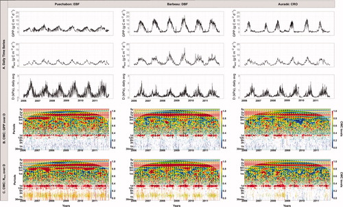
Fig. 9. Cross-wavelet coherence (CWC) analysis of GPP (B) and R_eco (C) with θ_EW at three sites (Puechabon, Barbeau and Auradé) from 2006 to 2011. The monthly time series of variables (A) are presented together with the corresponding scalograms of CWC.

For the three sites selected, Figs. 8 and 9 show the time series of GPP, R_eco, D and θ_EW together with cross-coherence spectra between GPP or R_eco and D (Fig. 8) or θ_EW (Fig. 9), from 2006 to 2011. The annual harmonic mode — or the annual cycle — showed the dominant effect of D and θ_EW on GPP and R_eco for the three sites as seen by the continuous high coherence (red colour) from 2006 to 2011. At higher frequencies, the daily cycle was marked by a strong coherence with D of both GPP and R_eco at all sites. At the day period, the CWC between θ_EW and R_eco was substantial in the cropland only. For intermediate periods (week to 6 months), the relationship between CO₂ flux and driving variables was highly non-linear in the modes 1 week to 2 months, as evidenced by the spectral gap between the day and week periods. This gap was however discontinuous for D, for which coherence peaks were observed sporadically during growing seasons. Hotspots of high coherence were detected for periods from a month to 6 months and will be described further below, first for the D and second for θ_EW.

The D cross-coherences with GPP and R_eco were roughly similar. The strong common power (red colour) with GPP at the 1-day period was observed during the growing season only. For the EBF site, the 1-day correlation was attenuated during winter, consistent with the smaller variations in D. At this 1-day period, GPP and D were in phase (arrow pointing up right) and GPP attained its maximum between 2 and 6 hours ahead of D (+π/12 and +π/4) (see Fig. S2). This was expected because D lagged 2 to 3 hours behind incident S_d. At 1-week to 2-month periods, correlations between GPP and D were weaker and phase relationships were more chaotic for the three sites. However, some localized high coherences spots were observed at intermediate scales in the EBF when θ_EW was not limiting (spring-summer 2007, spring 2011). In most of these situations, GPP and D were in phase with zero lag observed. At longer periods, (1 to 6 months) correlation hotspots between GPP and D were exhibited for the three sites. These seasonal hotspots were well individualized during the DBF growing seasons with GPP lagging behind D by an angle of 7π/4, that is about one week. The springs of 2006 and 2009 correlation hotspots were instead at the seasonal scale (4-month period), during which GPP and D were in anti-phase, D leading GPP by an angle of 3π/4 (∼1 month). In the EBF and cropland type, GPP and D are also correlated at periods of from 3 to 6 months. However, the GPP-D correlation was intermittently lost in the EBF, e.g., in spring 2008, both winter/spring 2009 and 2011, and in the crop site during winters of 2007, 2008, 2011. At one-year period, the three sites presented a strong correlation between GPP and D. The DBF signals were synchronized, while GPP led D by 3 months (+π/4 angle) in EBF and 4 months in the cropland (+π/3 angle).

The coherences of θ_EW with GPP and R_eco were also similar between sites showing two typical frequencies at day⁻¹ and year⁻¹ frequencies. Indeed, the coherence was highest at frequency bands and dates where θ_EW co-varied with GPP or R_eco. Similar co-occurring bands were observed at higher frequencies in the crop site, where the soil is shallowest. As for D, the GPP (R_eco) – θ_EW cross-power showed seasonal discontinuities at 1-day period related to the phenology of the canopies. A spectral gap appeared between the week and month periods where rare, discontinuous, coherence hotspots occurred. At periods from 1 to 6 months, some scattered, discontinuous coherence hotspots emerged during 2006–2011; these were consistent with the θ_EW power spectrum that showed its maximal power at these frequencies.

4. Discussion

We have based our data analyses upon homogenized time series of net CO₂ fluxes and their components, GPP and R_eco, and their relationship with independent drivers. The primary goal was not to maximize the fraction of variance explained but rather to examine the variability of fluxes as explained by climate drivers and the correlation patterns among PFTs. We limit our analysis to French sites under temperate and Mediterranean climates during the period, 2006–2011, for which a common 6-year long time series of raw data could be homogenized and processed. Our main findings concern the contribution of climate variables to the CO₂ fluxes among five PFTs, the relationship between the temporal variations of GPP, R_eco and the resulting NEE with climate, soil characteristics, PFT and management. Based on the RF and spectral analyses, they confirm the previous conclusions and intuitive results reached by the pioneering spectral analyses of ecosystem fluxes (Baldocchi et al. (2001), Katul et al. (2001) and Stoy et al. (2005, 2009)).

4.1. Contribution of environmental variables

The similarity between the PFTs in the distribution of the half-hourly CO₂ flux variances among contributors was assigned to the ubiquitous biological processes involved in the C3 photosynthesis metabolism: CO₂ diffusion through stomata and mesophyll, light absorption by chlorophyll antenna, the Calvin enzymatic cycle and RuBisCO kinetics. The high frequency dependency of these processes on incident light, temperature and CO₂ concentration is well characterized. Furthermore, such processes have been shown to integrate straightforwardly from the cell to the leaf and canopy levels, with relatively few upscaling effects (Farquhar et al. 1989; Rayment et al. 2002). Such processes respond to environmental drivers with time constants of minutes to an hour (Vialet-Chabrand et al. 2017) so that cross-variations of CO₂ fluxes with climate variables are expected to occur from minutes to decades. Since the RF analysis reveals only the direct effect of environmental variables at a 30-minute time-step, we should expect that a convergence among PFTs emerges from the ranking of driving variables by the RF algorithm.

The RF results are consistent with the conclusions reached by previous studies regarding the control of GPP, R_eco and NEE at high frequency (Baldocchi et al. 2001; Stoy et al. 2009; Ouyang et al. 2014). Here, the differential role among PFTs of hydrological drivers such as D and θ_EW on GPP and NEE is also apparent. Besides increasing atmospheric demand for evapotranspiration, increasing D has been assigned to stomata closure in response to increased atmospheric dryness (Farquhar 1978; Medlyn et al. 2011; Novick et al. 2016); although not necessarily through a direct effect of D (Damour et al. 2010). High values of D have been widely observed to coincide with stomatal closure and GPP decrease (Oren et al. 1999; Fu et al., 2018). D is therefore likely to control the CO₂ fluxes more tightly for those PFTs which expose the canopy foliage to high values of D for longer periods, such as the evergreen ecosystems at Puechabon and Le Bray in a warmer environment (Rambal et al. 2003). The D control was much less tight under wetter climates and canopies, e.g., the DBF Barbeau site and the alpine grassland at Laqueuille.

Soil drought also affects photosynthesis by degrading the plant and leaf water status, leading to stomatal closure, impaired growth, leaf shedding and ultimately xylem damage and plant mortality (Bréda et al. 2006; Granier et al. 2007). Soil water stress at θ_EW lower than 0.4 is reported to affect photosynthesis (Granier et al. 1999, 2000). This condition occurred on average on 115, 61 and 54 days for Puechabon (Mediterranean), Barbeau (temperate), and Auradé (crop), respectively, between 2006 and 2011. In the holm oak stand of Puechabon, Pita et al. (2013) showed a low GPP with low diurnal variability in accordance with a strong stomatal control caused by the severe water stress. This difference among sites and climates explains our RF analysis conclusions regarding the between-site differences. The soil water, θ_EW, is controlled by precipitation, runoff and water uptake by plants, but its variations are dampened by the soil water holding capacity. This combination of controls shifts its power scale pattern towards lower frequencies than those of D, a difference also observed in arid ecosystems by Jia et al. (2018). The θ_EW power gap in the high frequency range is thus more pronounced where the soil water holding capacity is large, e.g., in the old growth sessile oak stand at Barbeau (∼170 mm) as compared to the cropland Auradé (∼60 mm).

Compared to GPP, the situation is different for R_eco, which is controlled by diffusion and other transport processes intervening between the source metabolic activity and putative decarbonation processes in the soil and aboveground biomass. Indeed, not only the R_eco-T_air but also the R_eco-θ_EW correlation is explained at least partly by a causal relationship, with an effect of temperature and moisture at periods from an hour to months and a year (e.g., Janssens et al. 2001; Vargas et al. 2010a; Sierra et al. 2015). However, the correlation between half-hourly values of R_eco and θ_EW as observed at all sites might be partly coincidental, because respiration and soil moisture vary seasonally in parallel; they show lesser variations in winter when soil is cold and water-saturated, and larger variations during the growing season (Vargas et al. 2010b).

For the functional types with a discontinuous vegetation cover (Barbeau, Auradé and Laqueuille), the RF ranking of the air temperature, just after the radiation, indirectly suggests the role phenology played in the temporal pattern of GPP and therefore NEE (White et al. 1999). Interestingly, we observed that wind speed and CO₂ concentration above the canopy co-varied more closely with GPP in smoother canopies (Auradé and Laqueuille). This observation could be explained by the contrasting atmospheric coupling of forest, grasslands and croplands: in low vegetation, turbulence is less developed and the aerodynamic transfer less efficient, i.e., the vegetation is decoupled from the atmosphere. This process leads to the smoother canopies having a larger diel variation of CO₂ concentration that is synchronized and opposite to GPP variations. Therefore, we cannot conclude a direct influence of CO₂ on GPP through enhanced photosynthesis as has been suggested by Fernández-Martínez et al. (2017).

The percentage of variance explained by climate variables in the RF analysis decreased with the integration timespan, confirming that other variables or biotic parameters or delayed effects contribute to the monthly to yearly variability of CO₂ fluxes. Using regression algorithms with the machine learning approach to predict NEE, R_eco and GPP in all types of ecosystems (ENF, DBF, EBF, grasslands, croplands, etc…), Tramontana et al. (2016) were led to similar conclusions. This finding suggests that additional explanatory variables must be introduced to capture CO₂ flux variability at low frequency, especially at sites with no clear seasonal cycle as in evergreen broadleaf forest and crops. In different forest ecosystems (ENF, DBF and EBF), Urbanski et al. (2007); Delpierre et al. (2012) and Ouyang et al. (2014) showed that the direct influence of hydroclimatic drivers on canopy fluxes, especially NEE, was masked at longer time scales by the effects of canopy dynamics, photosynthetic thermal acclimation and ecosystem disturbances. As shown here by the RF analysis across integration times, several studies confirmed that climatic variables explain a large fraction of the variance of CO₂ fluxes, up to 80%, at high frequency (30-minute flux averages) (Loescher et al. 2003; Hollinger et al. 2004; Moffat et al. 2010), but can be reduced to an explained variance of 50% when scaled to longer time intervals (Law et al. 2002; Luyssaert et al. 2007b). Indeed, the RF analyses cannot account for the putative time lag and memory effects on NEE, GPP and R_eco (Papale et al. 2015) that might arise from the transfer of carbon from photosynthesis (GPP) to biomass and soil respiration (R_eco) and its variation between PFTs, seasons and species (Dannoura et al. 2011; Vargas et al. 2011).

The main explanation for the uneven RF performances among PFTs is their specific disturbance regimes. The lowest score obtained in the cropland site might be due to management practice (sowing dates) and disturbance (soil preparation, harvest) which are indeed crucial but not accounted for by either the RF or spectral analyses. The long-term effects of disturbances such as management and extreme events (heatwaves, storms and prolonged drought) were also not revealed by our RF analysis (Amiro et al. 2010; Moreaux et al. 2011; Buysse et al. 2017). As no biotic parameters were selected in the present analysis, our results are not overestimated, since as we discussed above, these biotic parameters are known to be relatively important in explaining flux variability, depending on the time scales considered. At the Auradé site, a supplementary test showed an increase up to 92.8% in the GPP variance explained when the vegetation structure and dynamics, such as LAI, was included, as compared to the initial 64.9% otherwise (data not shown) (Ouyang et al. 2014). Missing soil properties and carbon pools in the RF analysis may also explain its lower performance with increasing integration time in the two ecosystems investigated over a range of time scales.

4.2. Temporal behaviour of CO₂ flux variance partitioning

Our spectral analysis confirms previous conclusions extracted from the Fluxnet dataset (Stoy et al. 2009). Both our cross-coherence analysis across temporal scales and our RF analysis confirm the changes in importance of climate drivers on ecosystem CO₂ fluxes, GPP and R_eco, with decreasing time frequency. An important result of the RF analysis is to confirm the changes in importance of climate drivers of ecosystem CO₂ fluxes, GPP and R_eco, with decreasing time frequencies commonly observed in literature. This conclusion is also supported by the cross-coherence analysis across temporal scales. The variance of half-hourly ecosystem fluxes exceeded the variance of driving variables, as observed previously by Katul et al. (2001) at the Harvard Forest site and by Ouyang et al. (2014) in another temperate broadleaf forest in Ohio. It is generally dampened at longer periods, from weeks to a year, though Ouyang et al. (2014) observed a secondary power peak of NEE at 6-month period when compared with air temperature and incident light. The attenuation of the power of CO₂ fluxes at low frequency has been interpreted as the control of CO₂ fluxes by biological factors and the effects of synoptic weather patterns. Richardson et al. (2007) showed that 40% of the variance in modelled annual NEE can be attributed to variation in environmental drivers, and 55% to variation in the biotic drivers. Going through different time scales, Stoy et al. (2005) and Ouyang et al. (2014) concluded similarly that the control of NEE, GPP and R_eco changes as the integration timespan increases from day to season and to year. They found that the incident downward flux density of photosynthetically active radiation, followed by air vapour pressure saturation deficit dominated at a daily scale whereas soil water, temperature or stand characteristics were most influential at seasonal and annual scales. Furthermore, our spectral analysis shows that the time series of CO₂ flux power spectra over years are related to the canopy phenology and are markedly different for the studied PFTs. Our results closely confirm those obtained by a similar statistical analysis in a drought-stressed mixed ecosystem where soil moisture appeared as the most relevant predictor of GPP (Fares et al. 2013). Their ENF, which was planted with ponderosa pine, exhibited results with the same ranking order as we found for our ENF, the maritime pine ecosystem Le Bray.

The spectral analysis also showed the similarity of the power spectra of GPP and NEE from half-hourly to 1-month scales, and to a lesser extent at lower frequencies (Hong and Kim 2011; Jia et al. 2018). The GPP and R_eco power scale-wise patterns are clearly distinguishable from each other and confirm therefore that NEE diel to monthly variability is dominated by GPP independent of the PFT and climate type (Stoy et al. 2005, 2009; Luyssaert et al. 2007a; Ouyang et al. 2014; Jia et al. 2018). We cannot exclude, however, a putative influence of R_eco on NEE at longer time scales, 6-month to a year, although Luyssaert et al. (2007b) showed also that annual NEE anomalies in forests were created by anomalies in GPP and Fu et al. (2019) recently extended this conclusion to 66 sites. The contrasted scale-wise power of GPP and R_eco shows that their functional link has actually only a minor influence, if any. We think this is due to R_eco, the bulk CO₂ emission from the ecosystem, being the end process of the biological part of the carbon cycle and results from a combination of metabolic and transport processes occurring all along the soil-plant continuum (Sierra et al. 2015; Moya et al. 2019). Each respiratory source is using photosynthetic organic carbon fixed by the carboxylation of Ribulose, but the transfer time may vary widely between leaf respiration which can follow assimilation within minutes, to coarse woody debris mineralization which is lagged by months to years. These delays may obscure the functional link between GPP and R_eco and their respective temporal patterns. In addition, and contrary to the photosynthesis, which occurs only in the canopy foliage, the processes involved in the ecosystem respiration are located in above and belowground parts of the vegetation and through soil microbes which are subjected to a wide range of temperature and moisture. This positioning makes the relationship between R_eco and bulk climate variables more complex than the GPP’s. Last, the ecosystem respiration continues at night and during the dormant season; this may contribute to its power enrichment at intermediates scales and attenuation at high frequency as compared with GPP.

The 6-year period covered by our spectral analyses allowed us to examine how the power spectrum of fluxes, micrometeorological variables and their correlation have been changing from year to year. The soil water was intermittently correlated with both GPP and R_eco at intermediate (from twice a week to seasonal) frequencies especially at the end of summer periods and at the 1-yr period for the three ecosystems studied. On the contrary, GPP and R_eco were highly correlated to D at the 1-day and 1-yr periods in the three ecosystems with PFT-specific dynamics. For the evergreen broadleaf forest, Puechabon, GPP and R_eco were almost continuously in coherence with D at 3-month and 6-month periods; which is not the case in the deciduous forest and the cropland, which are marked by a canopy seasonality and for which GPP and R_eco were intermittently uncorrelated at intermediate frequencies. Here, the comparison of spectral power and coherences among PFT showed that the canopy phenology is a key characteristic for assessing the dynamic effects of climate drivers across time scales. As expected, the power of CO₂ fluxes and D co-vary with a larger magnitude in spring and summer and least in winter. Less intuitively the scalograms of the cropland revealed some periods where D variations are high but vegetation absent (late summer) and conversely, where D variations are lowest but vegetation is present (winter wheat). Here, the dynamics of the GPP-D cross-coherence clearly depends on the sowing date and leaf area development, and thus ultimately on management practice. This is of course not the case in the deciduous broadleaf forest since GPP-D cross-coherence coincides with the growing season and no management operations happened for the period considered. Accordingly, accounting for the LAI temporal variations would substantially improve the representation of CO₂ flux variability (Hong and Kim 2011; Delpierre et al. 2012; Stoy et al. 2013; Jia et al. 2018).

5. Conclusion

The empirical approaches that we used here, such as the Random Forest approach and spectral analysis, are useful tools for investigating temporal variations in ecological variables but have limited use for disentangling their drivers and causal chain, even when accounting for the phase effects. The canopy photosynthesis GPP appears as the primary process controlling the temporal changes of CO₂ exchange from the ecosystems considered, in accordance with the fact that it precedes the other carbon emission processes. The R_eco scale-wise variability is conversely clearly disconnected from the GPP: that may be explained by the nature of its complex spatial distribution and multiple sources. The differing phenology of the PFTs is a key characteristic governing their temporal variability. The management itself introduces a supplementary complexity in the time-frequency control of carbon fluxes as observed in the cropland, where management modifies the vegetation dynamics at intra-annual periods. This effect might also be present in forest but at lower frequencies since there, main operations (thinning, harvest, etc) occur at longer periods (5–10 years).

Understanding the impacts of biotic and abiotic variables on ecosystem fluxes and their temporal variability is still challenging due to the nature of the impacts. As pointed out by Stoy et al. (2009), improving the assessment of biotic and abiotic variables involved in the temporal control of CO₂ fluxes might benefit from using the upcoming generation of standardized long-term eddy covariance observations, e.g., the ICOS Research Infrastructure in Europe. Multiple site comparative analysis on standardized data series with well-documented ancillary data on management and canopy conditions will allow a better separation of drivers on ecosystem CO₂ fluxes.

Acknowledgements

This work used meteorological and eddy covariance raw data obtained within the framework of European projects: Euroflux, Carboeuroflux, CarboEuropeIP, CarboAge, GHG Europe, IMECC. VM acknowledges the financial support from the national agency ADEME for the eddy covariance data processing and harmonization within the CESEC project (PI: B. Longdoz), as well as the financial support from the European Union’s Horizon 2020 research for the RINGO project (grant agreement No 730944). The authors would like to thank all the PIs and technicians (e.g. Karim Piquemal, Franck Granouillac, Bartosz Zawilski and Nicole Ferroni) of the eddy covariance sites, and site collaborators involved in ICOS-France who are not included as co-authors of this paper and finally the support of the ‘Nouvelle Aquitaine’ region, the Regional Spatial Observatory (OSR), the CNRS (Centre National de la Recherche Scientifique) and the CNES (Centre National d’ Etudes Spatiales). The authors also thank John Gash for editing the article for style and grammar that improved the readability of the article.

Disclosure statement

No potential conflict of interest was reported by the authors.

References

- Ahlström, A., Raupach, M. R., Schurgers, G., Smith, B., Arneth, A., and co-authors. 2015. Carbon cycle. The dominant role of semi-arid ecosystems in the trend and variability of the land CO2 sink. Science 348, 895–899. doi:10.1126/science.aaa1668
- Allard, V., Ourcival, J. M., Rambal, S., Joffre, R. and Rocheteau, A. 2008. Seasonal and annual variation of carbon exchange in an evergreen Mediterranean forest in southern France. Glob. Change Biol. 14, 714–725. doi:10.1111/j.1365-2486.2008.01539.x
- Amiro, B. D., Barr, A. G., Barr, J. G., Black, T. A., Bracho, R., and co-authors. 2010. Ecosystem carbon dioxide fluxes after disturbance in forests of North America. J. Geophys. Res 115, G00K02, doi:10.1029/2010JG001390
- Aubinet, M., Hurdebise, Q., Chopin, H., Debacq, A., De Ligne, A., and co-authors. 2018. Inter-annual variability of Net Ecosystem Productivity for a temperate mixed forest: A predominance of carry-over effects? Agric. For. Meteorol. 262, 340–353. doi:10.1016/j.agrformet.2018.07.024
- Baldocchi, D. 2008. Breathing” of the terrestrial biosphere: lessons learned from a global network of carbon dioxide flux measurement systems. Aust. J. Bot. 56, 1. doi:10.1071/BT07151
- Baldocchi, D., Chu, H. and Reichstein, M. 2018. Inter-annual variability of net and gross ecosystem carbon fluxes: A review. Agric. For. Meteorol. 249, 520–533. doi:10.1016/j.agrformet.2017.05.015
- Baldocchi, D., Falge, E. and Wilson, K. 2001. A spectral analysis of biosphere–atmosphere trace gas flux densities and meteorological variables across hour to multi-year time scales. Agric. For. Meteorol. 107, 1–27. doi:10.1016/S0168-1923(00)00228-8
- Béziat, P., Ceschia, E. and Dedieu, G. 2009. Carbon balance of a three crop succession over two cropland sites in South West France. Agric. For. Meteorol. 149, 1628–1645. doi:10.1016/j.agrformet.2009.05.004
- Bréda, N., Huc, R., Granier, A. and Dreyer, E. 2006. Temperate forest trees and stands under severe drought: a review of ecophysiological responses, adaptation processes and long-term consequences. Ann. For. Sci. 63, 625–644. doi:10.1051/forest:2006042
- Breiman, L. 2001. Random forests. Mach. Learn. 45, 5–32. doi:10.1023/A:1010933404324
- Burba, G. G., Mc Dermitt, D. K., Grelle, A., Anderson, D. J. and Xu, L. 2008. Addressing the influence of instrument surface heat exchange on the measurements of CO2 flux from open-path gas analyzers. Glob. Change Biol. 14, 1854–1876. doi:10.1111/j.1365-2486.2008.01606.x
- Buysse, P., Bodson, B., Debacq, A., De Ligne, A., Heinesch, B., and co-authors. 2017. Carbon budget measurement over 12 years at a crop production site in the silty-loam region in Belgium. Agric. For. Meteorol 246, 241–255. doi:10.1016/j.agrformet.2017.07.004
- Cabon, A., Mouillot, F., Lempereur, M., Ourcival, J.-M., Simioni, G. and co-authors. 2018. Thinning increases tree growth by delaying drought-induced growth cessation in a Mediterranean evergreen oak coppice. For. Ecol. Manag. 409, 333–342. doi:10.1016/j.foreco.2017.11.030
- Chu, H., Baldocchi, D. D., John, R., Wolf, S. and Reichstein, M. 2017. Fluxes all of the time? A primer on the temporal representativeness of FLUXNET. J. Geophys. Res. Biogeosci. 122, 289–307. doi:10.1002/2016JG003576
- Ciais, P., Reichstein, M., Viovy, N., Granier, A., Ogée, J., and co-authors. 2005. Europe-wide reduction in primary productivity caused by the heat and drought in 2003. Nature 437, 529–533. doi:10.1038/nature03972
- Damour, G., Simonneau, T., Cochard, H. and Urban, L. 2010. An overview of models of stomatal conductance at the leaf level. Plant Cell Environ. 33, 1419–1438.
- Dannoura, M., Maillard, P., Fresneau, C., Plain, C., Berveiller, D., and co-authors. 2011. In situ assessment of the velocity of carbon transfer by tracing 13 C in trunk CO2 efflux after pulse labelling: variations among tree species and seasons. New Phytol. 190, 181–192. doi:10.1111/j.1469-8137.2010.03599.x
- Delpierre, N. 2009. Etude du déterminisme des variations interannuelles des échanges carbonés entre les écosystèmes forestiers européens et l’atmosphère: une approche basée sur la modélisation des processus (thesis). Paris 11.
- Delpierre, N., Berveiller, D., Granda, E. and Dufrêne, E. 2016. Wood phenology, not carbon input, controls the interannual variability of wood growth in a temperate oak forest. New Phytol. 210, 459–470. doi:10.1111/nph.13771
- Delpierre, N., Soudani, K., François, C., Köstner, B., Pontailler, J.-Y., and co-authors. 2009. Exceptional carbon uptake in European forests during the warm spring of 2007: a data–model analysis. Glob. Change Biol. 15, 1455–1474. doi:10.1111/j.1365-2486.2008.01835.x
- Delpierre, N., Soudani, K., François, C., Le Maire, G., Bernhofer, C., and co-authors. 2012. Quantifying the influence of climate and biological drivers on the interannual variability of carbon exchanges in European forests through process-based modelling. Agric. For. Meteorol. 154-155, 99–112. doi:10.1016/j.agrformet.2011.10.010
- Dou, X., Chen, B., Black, T. A., Jassal, R. S. and Che, M. 2015. Impact of nitrogen fertilization on forest carbon sequestration and water loss in a chronosequence of three Douglas-Fir stands in the Pacific Northwest. Forests 6, 1897–1921. doi:10.3390/f6061897
- Dou, X., Yang, Y. and Luo, J. 2018. Estimating forest carbon fluxes using machine learning techniques based on eddy covariance measurements. Sustainability 10, 203. doi:10.3390/su10010203
- Etchanchu, J., Rivalland, V., Gascoin, S., Cros, J., Tallec, T., and co-authors. 2017. Effects of high spatial and temporal resolution Earth observations on simulated hydrometeorological variables in a cropland (southwestern France). Hydrol. Earth Syst. Sci. 21, 5693–5708. doi:10.5194/hess-21-5693-2017
- Falge, E., Baldocchi, D., Olson, R., Anthoni, P., Aubinet, M., and co-authors. 2001. Gap filling strategies for defensible annual sums of net ecosystem exchange. Agric. For. Meteorol 107, 43–69. doi:10.1016/S0168-1923(00)00225-2
- Fares, S., Vargas, R., Detto, M., Goldstein, A. H., Karlik, J. and co-authors. 2013. Tropospheric ozone reduces carbon assimilation in trees: estimates from analysis of continuous flux measurements. Glob. Chang. Biol. 19, 2427–2443. doi:10.1111/gcb.12222
- Farquhar, G. D. 1978. Feedforward responses of stomata to humidity. Functional Plant Biol. 5, 787–800. doi:10.1071/PP9780787
- Farquhar, G. D., Walker, D. A. and Osmond, C. B. 1989. Models of integrated photosynthesis of cells and leaves. Philos. Trans. R. Soc. Lond. B Biol. Sci. 323, 357–367.
- Fernández-Martínez, M., Vicca, S., Janssens, I. A., Ciais, P., Obersteiner, M., and co-authors. 2017. Atmospheric deposition, CO2, and change in the land carbon sink. Sci. Rep. 7, 9632. doi:10.1038/s41598-017-08755-8
- Fratini, G., Ibrom, A., Arriga, N., Burba, G. and Papale, D. 2012. Relative humidity effects on water vapour fluxes measured with closed-path eddy-covariance systems with short sampling lines. Agric. For. Meteorol. 165, 53–63. doi:10.1016/j.agrformet.2012.05.018
- Fu, Z., Gerken, T., Bromley, G., Araújo, A., Bonal, D., and co-authors. 2018. The surface-atmosphere exchange of carbon dioxide in tropical rainforests: Sensitivity to environmental drivers and flux measurement methodology. Agric. For. Meteorol. 263, 292–307. doi:10.1016/j.agrformet.2018.09.001
- Fu, Z., Stoy, P. C., Poulter, B., Gerken, T., Zhang, Z., and co-authors. 2019. Maximum carbon uptake rate dominates the interannual variability of global net ecosystem exchange. Glob. Chang. Biol. 25, 3381–3394. doi:10.1111/gcb.14731
- Gash, J. H. C. and Culf, A. D. 1996. Applying a linear detrend to eddy correlation data in realtime. Boundary-Layer Meteorol. 79, 301–306. doi:10.1007/BF00119443
- Granier, A., Bréda, N., Biron, P. and Villette, S. 1999. A lumped water balance model to evaluate duration and intensity of drought constraints in forest stands. Ecol. Model 116, 269–283. doi:10.1016/S0304-3800(98)00205-1
- Granier, A. and Loustau, D. 1994. Measuring and modelling the transpiration of a maritime pine canopy from sap-flow data. Agric. For. Meteorol 71, 61–81. doi:10.1016/0168-1923(94)90100-7
- Granier, A., Loustau, D. and Br⏧da, N. 2000. A generic model of forest canopy conductance dependent on climate, soil water availability and leaf area index. Ann. For. Sci. 57, 755–765. doi:10.1051/forest:2000158
- Granier, A., Reichstein, M., Bréda, N., Janssens, I. A., Falge, E., and co-authors. 2007. Evidence for soil water control on carbon and water dynamics in European forests during the extremely dry year: 2003. Agric. For. Meteorol 143, 123–145. doi:10.1016/j.agrformet.2006.12.004
- Hollinger, D. Y., Aber, J., Dail, B., Davidson, E. A., Goltz, S. M., and co-authors. 2004. Spatial and temporal variability in forest–atmosphere CO2 exchange. Global Change Biol. 10, 1689–1706. doi:10.1111/j.1365-2486.2004.00847.x
- Hong, J. and Kim, J. 2011. Impact of the Asian monsoon climate on ecosystem carbon and water exchanges: a wavelet analysis and its ecosystem modeling implications. Glob. Change Biol. 17, 1900–1916. doi:10.1111/j.1365-2486.2010.02337.x
- Horst, T. W. and Lenschow, D. H. 2009. Attenuation of scalar fluxes measured with spatially-displaced sensors. Boundary-Layer Meteorol. 130, 275–300. doi:10.1007/s10546-008-9348-0
- Janssens, I. A., Lankreijer, H., Matteucci, G., Kowalski, A. S., Buchmann, N., and co-authors. 2001. Productivity overshadows temperature in determining soil and ecosystem respiration across European forests. Global Change Biol. 7, 269–278. doi:10.1046/j.1365-2486.2001.00412.x
- Jarosz, N., Brunet, Y., Lamaud, E., Irvine, M., Bonnefond, J.-M. and co-authors. 2008. Carbon dioxide and energy flux partitioning between the understorey and the overstorey of a maritime pine forest during a year with reduced soil water availability. Agric. For. Meteorol. 148, 1508–1523. doi:10.1016/j.agrformet.2008.05.001
- Jia, X., Zha, T., Gong, J., Zhang, Y., Wu, B., and co-authors. 2018. Multi-scale dynamics and environmental controls on net ecosystem CO2 exchange over a temperate semiarid shrubland. Agric. For. Meteorol. 259, 250–259. doi:10.1016/j.agrformet.2018.05.009
- Jung, M., Reichstein, M., Schwalm, C. R., Huntingford, C., Sitch, S., and co-authors. 2017. Compensatory water effects link yearly global land CO2 sink changes to temperature. Nature 541, 516–520. doi:10.1038/nature20780
- Katul, G., Lai, C.-T., Schäfer, K., Vidakovic, B., Albertson, J., and co-authors. 2001. Multiscale analysis of vegetation surface fluxes: from seconds to years. Adv. Water Resour. 24, 1119–1132. doi:10.1016/S0309-1708(01)00029-X
- Klumpp, K., Tallec, T., Guix, N. and Soussana, J.-F. 2011. Long-term impacts of agricultural practices and climatic variability on carbon storage in a permanent pasture. Glob. Change Biol. 17, 3534–3545. doi:10.1111/j.1365-2486.2011.02490.x
- Law, B. E., Falge, E., Gu, L., Baldocchi, D. D., Bakwin, P., and co-authors. 2002. Environmental controls over carbon dioxide and water vapor exchange of terrestrial vegetation. Agric. For. Meteorol. 113, 97–120. doi:10.1016/S0168-1923(02)00104-1
- Liaw, A. and Wiener, M. 2018. RandomForest Package, 2018. Breiman and Cutler’s Random Forests for Classification and Regression. 29pp. Online at: https://cran.r-project.org/web/packages/randomForest/randomForest.pdf
- Liu, Z., Ballantyne, A. P., Poulter, B., Anderegg, W. R. L., Li, W., and co-authors. 2018. Precipitation thresholds regulate net carbon exchange at the continental scale. Nat. Commun. 9, 3596. doi:10.1038/s41467-018-05948-1
- Loescher, H. W., Oberbauer, S. F., Gholz, H. L. and Clark, D. B. 2003. Environmental controls on net ecosystem-level carbon exchange and productivity in a Central American tropical wet forest. Global Change Biol. 9, 396–412. doi:10.1046/j.1365-2486.2003.00599.x
- Loustau, D. and Granier, A. 1993. Environmental control of water flux through maritime pine (Pinus pinaster Ait.). In: Water Transport in Plants under Climatic Stress (eds. M. Borghetti, J. Grace, A. Raschi). Cambridge University Press, Cambridge, 205–18 pp.
- Loustau, D., Bosc, A., Colin, A., Ogée, J., Davi, H., and co-authors. 2005. Modeling climate change effects on the potential production of French plains forests at the sub-regional level. Tree Physiol. 25, 813–823. doi:10.1093/treephys/25.7.813
- Luyssaert, S., Inglima, I., Jung, M., Richardson, A. D., Reichstein, M., and co-authors. 2007a. CO2 balance of boreal, temperate, and tropical forests derived from a global database. Global Change Biol. 13, 2509–2537. doi:10.1111/j.1365-2486.2007.01439.x
- Luyssaert, S., Janssens, I. A., Sulkava, M., Papale, D., Dolman, A. J., and co-authors. 2007b. Photosynthesis drives anomalies in net carbon-exchange of pine forests at different latitudes. Global Change Biol. 13, 2110–2127. doi:10.1111/j.1365-2486.2007.01432.x
- Marcolla, B., Cescatti, A., Manca, G., Zorer, R., Cavagna, M., and co-authors. 2011. Climatic controls and ecosystem responses drive the inter-annual variability of the net ecosystem exchange of an alpine meadow. Agric. For. Meteorol 151, 1233–1243. doi:10.1016/j.agrformet.2011.04.015
- Mauder, M. and Foken, T. 2004. Documentation and Instruction Manual of the Eddy Covariance Software Package TK2 – Universität Bayreuth. Abt. Mikrometeorologie, Arbeit-Sergebnisse 26, 44. pp. (Print: ISSN 1614-8916; Internet:ISSN 1614-8926).
- McInerney, D. and Nieuwenhuis, M. 2009. Comparative analysis of kNN and decision tree methods for the Irish National Forest Inventory. Int J. Remote Sens 30, 4937–4955. doi:10.1080/01431160903022936
- Medlyn, B. E., Duursma, R. A., Eamus, D., Ellsworth, D. S., Prentice, I. C., and co-authors. 2011. Reconciling the optimal and empirical approaches to modelling stomatal conductance. Glob. Change Biol 17, 2134–2144. doi:10.1111/j.1365-2486.2010.02375.x
- Moffat, A. M., Beckstein, C., Churkina, G., Mund, M. and Heimann, M. 2010. Characterization of ecosystem responses to climatic controls using artificial neural networks. Glob. Change Biol. 16, 2737–2749. doi:10.1111/j.1365-2486.2010.02171.x
- Moncrieff, J., Clement, R., Finnigan, J. and Meyers, T. 2005. Averaging, detrending, and filtering of Eddy covariance time series. In: Handbook of Micrometeorology: A Guide for Surface Flux Measurement and Analysis, Atmospheric and Oceanographic Sciences Library (eds. X. Lee, W. Massman, B. Law). Springer, Dordrecht, Netherlands, 7–31 pp.
- Moncrieff, J. B., Massheder, J. M., de Bruin, H., Elbers, J., Friborg, T., and co-authors. 1997. A system to measure surface fluxes of momentum, sensible heat, water vapour and carbon dioxide. J. Hydrol., HAPEX-Sahel 188-189, 589–611. doi:10.1016/S0022-1694(96)03194-0
- Moreaux, V., Lamaud, É., Bosc, A., Bonnefond, J.-M., Medlyn, B. E. and co-authors. 2011. Paired comparison of water, energy and carbon exchanges over two young maritime pine stands (Pinus pinaster Ait.): effects of thinning and weeding in the early stage of tree growth. Tree Physiol. 31, 903–921. doi:10.1093/treephys/tpr048
- Morlet, J., Arens, G., Fourgeau, E. and Giard, D. 1982. Wave propagation and sampling theory—Part II: Sampling theory and complex waves. Geophysics 47, 222–236. doi:10.1190/1.1441329
- Mouillot, F., Rambal, S. and Lavorel, S. 2001. A generic process-based SImulator for meditERRanean landscApes (SIERRA): design and validation exercises. For. Ecol. Manag. 147, 75–97. doi:10.1016/S0378-1127(00)00432-1
- Moya, M. R., Sánchez-Cañete, E. P., Vargas, R., López-Ballesteros, A., Oyonarte, C., and co-authors. 2019. CO2 dynamics are strongly influenced by low frequency atmospheric pressure changes in semiarid grasslands. J. Geophys. Res. Biogeosci. 124, 902–917. doi:10.1029/2018JG004961
- Niu, S., Fu, Z., Luo, Y., Stoy, P. C., Keenan, T. F., and co-authors. 2017. Interannual variability of ecosystem carbon exchange: From observation to prediction. Global Ecol. Biogeogr. 26, 1225–1237. doi:10.1111/geb.12633
- Novick, K. A., Ficklin, D. L., Stoy, P. C., Williams, C. A., Bohrer, G., and co-authors. 2016. The increasing importance of atmospheric demand for ecosystem water and carbon fluxes. Nature Clim. Change 6, 1023–1027. doi:10.1038/nclimate3114
- Ogée, J., Brunet, Y., Loustau, D., Berbigier, P. and Delzon, S. 2003. MuSICA, a CO2, water and energy multilayer, multileaf pine forest model: evaluation from hourly to yearly time scales and sensitivity analysis. Global Change Biol. 9, 697–717. doi:10.1046/j.1365-2486.2003.00628.x
- Oren, R., Sperry, J. S., Katul, G. G., Pataki, D. E., Ewers, B. E., and co-authors. 1999. Survey and synthesis of intra- and interspecific variation in stomatal sensitivity to vapour pressure deficit. Plant Cell Environ. 22, 1515–1526. doi:10.1046/j.1365-3040.1999.00513.x
- Ouyang, Z., Chen, J., Becker, R., Chu, H., Xie, J., and co-authors. 2014. Disentangling the confounding effects of PAR and air temperature on net ecosystem exchange at multiple time scales. Ecol. Complex 19, 46–58. doi:10.1016/j.ecocom.2014.04.005
- Papale, D., Black, T. A., Carvalhais, N., Cescatti, A., Chen, J., and co-authors. 2015. Effect of spatial sampling from European flux towers for estimating carbon and water fluxes with artificial neural networks. J. Geophys. Res. Biogeosci. 120, 1941–1957. doi:10.1002/2015JG002997
- Papale, D. and Valentini, R. 2003. A new assessment of European forests carbon exchanges by eddy fluxes and artificial neural network spatialization. Global Change Biol. 9, 525–535. doi:10.1046/j.1365-2486.2003.00609.x
- Pereira, J. S., Mateus, J. A., Aires, L. M., Pita, G., Pio, C., and co-authors. 2007. Net ecosystem carbon exchange in three contrasting Mediterranean ecosystems - the effect of drought. Biogeosciences 4, 791–802. doi:10.5194/bg-4-791-2007
- Pita, G., Gielen, B., Zona, D., Rodrigues, A., Rambal, S., and co-authors. 2013. Carbon and water vapor fluxes over four forests in two contrasting climatic zones. Agric. For. Meteorol. 180, 211–224. doi:10.1016/j.agrformet.2013.06.003
- Rambal, S., Ourcival, J.-M., Joffre, R., Mouillot, F., Nouvellon, Y., and co-authors. 2003. Drought controls over conductance and assimilation of a Mediterranean evergreen ecosystem: scaling from leaf to canopy. Global Change Biol. 9, 1813–1824. doi:10.1111/j.1365-2486.2003.00687.x
- Rayment, M. B., Loustau, D. and Jarvis, P. J. 2002. Photosynthesis and respiration of black spruce at three organizational scales: shoot, branch and canopy. Tree Physiol. 22, 219–229. doi:10.1093/treephys/22.4.219
- Reichstein, M., Falge, E., Baldocchi, D., Papale, D., Aubinet, M., and co-authors. 2005. On the separation of net ecosystem exchange into assimilation and ecosystem respiration: review and improved algorithm. Global Change Biol. 11, 1424–1439. doi:10.1111/j.1365-2486.2005.001002.x
- Richardson, A. D., Hollinger, D. Y., Aber, J. D., Ollinger, S. V. and Braswell, B. H. 2007. Environmental variation is directly responsible for short- but not long-term variation in forest-atmosphere carbon exchange. Glob. Change Biol. 13, 788–803. doi:10.1111/j.1365-2486.2007.01330.x
- Rösch, A. and Schmidbauer, H. 2018. WaveletComp 1.1: A guided tour through the R package. Online at: https://CRAN.R-project.org/package=WaveletComp58pp.
- Shao, J., Zhou, X., Luo, Y., Li, B., Aurela, M., and co-authors. 2016. Direct and indirect effects of climatic variations on the interannual variability in net ecosystem exchange across terrestrial ecosystems. Tellus B Chem. Phys. Meteorol. 68, 30575. doi:10.3402/tellusb.v68.30575
- Sierra, C. A., Trumbore, S. E., Davidson, E. A., Vicca, S. and Janssens, I. 2015. Sensitivity of decomposition rates of soil organic matter with respect to simultaneous changes in temperature and moisture. J. Adv. Model. Earth Syst. 7, 335–356. doi:10.1002/2014MS000358
- Stoy, P. C., Dietze, M. C., Richardson, A. D., Vargas, R., Barr, A. G., and co-authors. 2013. Evaluating the agreement between measurements and models of net ecosystem exchange at different times and timescales using wavelet coherence: an example using data from the North American Carbon Program Site-Level Interim Synthesis. Biogeosciences 10, 6893–6909. doi:10.5194/bg-10-6893-2013
- Stoy, P. C., Katul, G. G., Siqueira, M. B. S., Juang, J.-Y., McCarthy, H. R., and co-authors. 2005. Variability in net ecosystem exchange from hourly to inter-annual time scales at adjacent pine and hardwood forests: a wavelet analysis. Tree Physiol. 25, 887–902. doi:10.1093/treephys/25.7.887
- Stoy, P. C., Richardson, A. D., Baldocchi, D. D., Katul, G. G., Stanovick, J., and co-authors. 2009. Biosphere-atmosphere exchange of CO2 in relation to climate: a cross-biome analysis across multiple time scales. Biogeosciences 6, 2297–2312. doi:10.5194/bg-6-2297-2009
- Torrence, C. and Compo, G. P. 1998. A practical guide to wavelet analysis. Bull. Am. Meteorol. Soc. 79, 18.
- Torrence, C. and Webster, P. J. 1999. Interdecadal changes in the ENSO–Monsoon System. J. Clim. 12, 12.
- Tramontana, G., Jung, M., Schwalm, C. R., Ichii, K., Camps-Valls, G., and co-authors. 2016. Predicting carbon dioxide and energy fluxes across global FLUXNET sites with regression algorithms. Biogeosciences 13, 4291–4313. doi:10.5194/bg-13-4291-2016
- Urbanski, S., Barford, C., Wofsy, S., Kucharik, C., Pyle, E., and co-authors. 2007. Factors controlling CO2 exchange on timescales from hourly to decadal at Harvard Forest. J. Geophys. Res. 112, G02020.
- Vargas, R., Baldocchi, D. D., Allen, M. F., Bahn, M., Black, T. A., and co-authors. 2010a. Looking deeper into the soil: biophysical controls and seasonal lags of soil CO2 production and efflux. Ecol. Appl. 20, 1569–1582. doi:10.1890/09-0693.1
- Vargas, R., Detto, M., Baldocchi, D. D. and Allen, M. F. 2010b. Multiscale analysis of temporal variability of soil CO2 production as influenced by weather and vegetation. Glob. Change Biol. 16, 1589–1605. doi:10.1111/j.1365-2486.2009.02111.x
- Vargas, R., Baldocchi, D. D., Bahn, M., Hanson, P. J., Hosman, K. P., and co-authors. 2011. On the multi-temporal correlation between photosynthesis and soil CO2 efflux: reconciling lags and observations. New Phytol. 191, 1006–1017. doi:10.1111/j.1469-8137.2011.03771.x
- Vialet-Chabrand, S. R. M., Matthews, J. S. A., McAusland, L., Blatt, M. R., Griffiths, H. and co-authors. 2017. Temporal dynamics of stomatal behavior: Modeling and implications for photosynthesis and water use. Plant Physiol. 174, 603–613. doi:10.1104/pp.17.00125
- Vickers, D. and Mahrt, L. 1997. Quality control and flux sampling problems for tower and aircraft data. J. Atmos. Oceanic Technol. 14, 512–526.(1997)014 < 0512:QCAFSP > 2.0.CO;2 doi:10.1175/1520-0426(1997)014<0512:QCAFSP>2.0.CO;2
- Vuichard, N., Soussana, J.-F., Ciais, P., Viovy, N. and Ammann, C, and co-authors. 2007. Estimating the greenhouse gas fluxes of European grasslands with a process-based model: 1. Model evaluation from in situ measurements. Glob. Biogeochem. Cycles 21, GB1004, doi:10.1029/2005GB002611.
- Webb, E. K., Pearman, G. I. and Leuning, R. 1980. Correction of flux measurements for density effects due to heat and water vapour transfer. QJ. Royal Met. Soc. 106, 85–100. doi:10.1002/qj.49710644707
- White, M. A., Running, S. W. and Thornton, P. E. 1999. The impact of growing-season length variability on carbon assimilation and evapotranspiration over 88 years in the eastern US deciduous forest. Int. J. Biometeorol. 42, 139–145. doi:10.1007/s004840050097
- Wilczak, J. M., Oncley, S. P. and Stage, S. A. 2001. Sonic Anemometer tilt correction algorithms. Bound.-Layer Meteorol. 99, 127–150. doi:10.1023/A:1018966204465
- Wohlfahrt, G., Fenstermaker, L. F. and Arone, J. A A. III. 2008. Large annual net ecosystem CO2 uptake of a Mojave Desert ecosystem. Global Change Biol. 14, 1475–1487. doi:10.1111/j.1365-2486.2008.01593.x
- Wutzler, T., Lucas-Moffat, A., Migliavacca, M., Knauer, J., Sickel, K., and co-authors. 2018. Basic and extensible post-processing of eddy covariance flux data with REddyProc. Biogeosciences 15, 5015–5030. doi:10.5194/bg-15-5015-2018