Optimal control and cost-effectiveness analysis of age-structured malaria model with asymptomatic carrier and temperature variability

Abstract

This paper presents an age-structured mathematical model for malaria transmission dynamics with asymptomatic carrier and temperature variability. The temperature variability function is fitted to the temperature data, and the malaria model is then fitted to the malaria cases and validated to check its suitability. Time-dependent controls were considered, including Long Lasting Insecticide Nets, treatment of symptomatic, screening and treatment of asymptomatic carriers and spray of insecticides. Pontryagin's Maximum Principle is used to derive the necessary conditions for optimal control of the disease. The numerical simulations of the optimal control problem reveal that the strategy involving the combination of all four controls is the most effective in reducing the number of infected individuals. Furthermore, the cost-effectiveness analysis shows that treatment of symptomatic, screening and treatment of asymptomatic carriers and insecticide spraying is the most cost-effective strategy to implement to control malaria transmission when available resources are limited.

Keywords:

• Age structure
• malaria
• asymptomatic carrier
• temperature
• optimal control
• cost-effectiveness

1. Introduction

Malaria is a vector-borne infectious disease caused by Plasmodium parasite and is transmitted by a bite of infected female anopheles mosquitoes. The disease is life-threatening, causing morbidity and mortality globally. In 2019, estimated malaria cases were 229 million and 40,900 deaths, with 67% deaths occurring in children under the age of five worldwide [30]. Tropical and subtropical regions of the world experience a large number of malaria cases [30]. This is because these regions experience unprecedented variations in temperature. Temperature affects the vector and parasite behaviour [6]. The mosquito feeds more frequently as temperature increases because blood is digested more quickly [6]. Furthermore, the average lifespan of a mosquito decreases rapidly when the temperature rises beyond [30${}^{\mathrm{o}}$C, 32${}^{\mathrm{o}}$C] [9]. Likewise, temperature affects malaria parasites inside the mosquito. Consequently, the maturation period decreases from nineteen days at 22${}^{\mathrm{o}}$C to eight days at 30${}^{\mathrm{o}}$C [12]. It is reported that mosquito and parasite biology are not only influenced by average temperature but also by the extent of temperature variability [11]. Fluctuations in temperature affect the spread of malaria by lowering or spreading up its rate of transmission [16]. Although changes in temperature influence the dynamics of malaria, other non-climatic factors such as age and asymptomatic carrier play a vital role in malaria dynamics [26]. Hence assessing the impact of temperature variability on the dynamics of malaria requires a better understanding of the role of these non-climatic factors and their combinations on the host-vector dynamics.

Numerous mathematical models have been developed to investigate the role of both non-climatic and climatic factors. For example, the studies of [2,10] considered age-structured model and Mwanga et al . [20] developed a two-age-structured SI model with an asymptomatic carrier. Temperature and rainfall were incorporated in [1,21]. Okuneye and Gumel [23] considered temperature and rainfall on malaria transmission dynamics in age-structured populations. The results suggest that anti-malaria control efforts should be intensified when malaria transmission is maximum.

Malaria is a preventable and curable disease. There is no single way to prevent malaria. However, there are different ways to reduce transmission, such as using treated nets, treating infected humans, and treating adulticide. Optimal control theory has been used in various studies to find a combination of control strategies to eradicate the disease. Mwanga et al. [20] considered four control strategies (Long Lasting Insecticide Nets(LLIN), treatment of symptomatic infections, screening and treatment of asymptomatic carriers and Indoor Residual Spraying (IRS)). Optimal control theory was then used to determine optimal control strategies to control the spread of malaria. Their results show that the disease can be brought to a stable disease-free equilibrium when all four controls are used. Okosun et al. [22] developed a malaria transmission model with three time-dependent controls. Olaniyi et al. [24] investigated optimal control strategies and cost-effectiveness analysis of malaria dynamics with partial immunity and protected travellers using ITNs, prophylaxis, treatment of infectious humans and vector control.

The effect of temperature variability with control strategies was also considered by Garba and Danbaba [11]. In their study, time-independent controls were used. Agusto [4] presented a malaria model that considers time-dependent control on malaria transmission dynamics with temperature variations. The study considered personal protection and mosquito reduction (larvicide and adulticide) strategies, and temperature ranges suitable for malaria transmission were determined. The authors suggested that the high use of larvicides and adulticides followed by moderate personal protection such as bed nets should be applied to control malaria. The control strategies incorporated in the model depend on the factors affecting transmission dynamics considered. Therefore, it is crucial to include more factors affecting malaria transmission dynamics to investigate control strategies to contain the disease.

This study considers an age-structured malaria transmission model with asymptomatic carrier and temperature variability. The aim is to investigate the combined effects of temperature variability on an age-structured population with asymptomatic carriers. The model further incorporates time-dependent control strategies to determine the control strategy that can best control the disease. Hence the model developed in this study differs from that in [20] by including exposed and recovered class in the host population and temperature variability. Also the model developed in this study deviates from [4] by incorporating an age-structured host population and asymptomatic carriers. It further differs from the study of Okuneye and Gumel [23] by considering asymptomatic carriers and time-dependent control strategies. In addition, it deviates from the study in [14] by incorporating temperature variability and time-dependent control strategies.

The paper is organized as follows–the model formulation and analysis of the model without temperature in Section 2. In Section 3 model with temperature-dependent parameters is fitted and validated. Section 4 focuses on formulating an optimal control problem and deriving the optimal system that characterizes the optimal control using Pontryagin's Maximum Principle. Numerical simulation and cost-effectiveness analysis are presented in Section 5. Finally, we conclude in Section 6.

2. Model formulation

The total human population $N_h$ is divided into two classes, under five years $N_c$ and five years and above $N_a$. The idea of grouping the human population into two groups have also been previously used by [3,10,14,20]. This is because children under five years are more prone to malaria than adults, since children have not yet developed immunity specific to the disease [27].

Each class is further subdivided into four compartments; susceptible $(S_i)$, exposed $(E_i)$, infectious $(I_i)$ and recovered class $(R_i)$, where $i=c,a$ represents under five and five years and above subpopulations respectively. Infectious class for five years and above comprises asymptomatic $A_a$ and symptomatic $I_a$. The asymptomatic class is the class of infectious individuals who do not show symptoms but can transmit the disease to mosquitoes. On the other hand, the symptomatic class is a class of infectious individuals who show symptoms and can infect mosquitoes. The rate of infection of a susceptible individual is ${\lambda }_i(T)=\frac{b(T){\beta }_i{S}_i{I}_m}{N_h}$ whereby $b(T)$ represents mosquito's biting rate, and ${\beta }_i$ is the proportion of bites by infectious mosquitoes on susceptible humans that produce infection. The biting rate is temperature-dependent because, at a warmer temperature, mosquitoes feed more frequently [8].

Once an individual is infected, individuals move to the exposed class $E_i$ for a few days before they become infectious. Individuals cannot transmit the parasite to susceptible mosquitoes at this stage since they do not have gametocytes. Exposed humans progress to infectious class at a rate ${\sigma }_i$ in which they can now infect susceptible mosquitoes. For the exposed class in the adult group, a proportion θ progresses to the symptomatic class, and the remaining $(1-\theta )$ joins the asymptomatic class. Symptomatic individuals ($I_c$ and $I_a$), through treatment or natural recovery with temporary immunity, move to the recovered class at a rate ${\gamma }_c$ and ${\gamma }_s$, respectively. Asymptomatic carriers recover naturally with temporary immunity and transition to recovered class at a rate ${\gamma }_a$. Temporary immune individuals lose immunity and become susceptible at a rate ${\eta }_i$. Individuals in every compartment suffer natural death at a rate ${\mu }_h$, and individuals in the infectious class die due to infection at a rate ${\delta }_i$ except for the asymptomatic class who are not harmed by the disease. Humans population is recruited by birth or immigration at a rate ${\mathrm{\Lambda }}_c$. Also, under five in every compartment may grow and move to the corresponding class in the five and above years group at a rate ζ.

The total adult mosquito population is divided into three compartments: susceptible $S_m$ exposed $E_m$ and infectious $I_m$. The birth rate for mosquitoes is temperature (T) dependent given by ${\mathrm{\Lambda }}_m(T)$. This is because temperature limits mosquito abundance [6]. The infection rate ${\lambda }_m(T)$ of a susceptible mosquito depends on the mosquito's biting rate $b(T)$ and the proportion of bites by susceptible mosquitoes on infected humans ($I_c$, $I_a$ and $A_a$) that results in infection ${\beta }_m$. Hence ${\lambda }_m(T)=\frac{b(T){\beta }_m{S}_m(I_c+I_a+r{A}_a)}{N_h}$ where r is a relative infectivity on an asymptomatic carrier as compared to symptomatic infections. During blood meals, susceptible mosquitoes take up gametocytes from infectious humans and progress into the exposed class. At this stage, they do not have sporozoites in their salivary gland and therefore are not infectious. When the gametocytes develop into sporozoites, mosquitoes are considered infectious. They move to the infectious class at a rate ${\sigma }_m(T)$, which is temperature-dependent as the maturation rate of the parasite within a mosquito depends on temperature. Mosquitoes in every class die naturally at a rate of ${\mu }_m(T)$. The death rate of mosquitoes depends on temperature (T) because the temperature can affect the lifespan of mosquitoes. The flow diagram of the model is depicted in Figure 1, and a description of the parameters is given in Table 1.

Figure 1. Flow diagram for the dynamics of malaria in the two age groups.

The bold arrow indicate the movements of individuals and mosquitoes from one compartment to the other, while the dash lines represent the interactions between humans and mosquitoes.

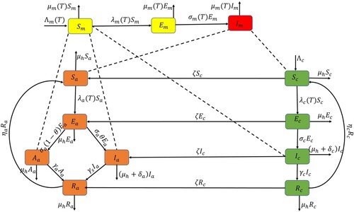
Table 1. Description of parameters used in the model Equation (1(1) $\begin{array}{r}\begin{array}{ll}{\displaystyle \frac{\mathrm{d}{S}_c}{\mathrm{d}t}}& ={\mathrm{\Lambda }}_c+{\eta }_c{R}_c-({\mu }_h+{\lambda }_c(T)+\zeta )S_c,\\ {\displaystyle \frac{\mathrm{d}{E}_c}{\mathrm{d}t}}& ={\lambda }_c(T)S_c-({\mu }_h+{\sigma }_c+\zeta )E_c,\\ {\displaystyle \frac{\mathrm{d}{I}_c}{\mathrm{d}t}}& ={\sigma }_c{E}_c-({\mu }_h+{\delta }_c+\zeta +{\gamma }_c)I_c,\\ {\displaystyle \frac{\mathrm{d}{R}_c}{\mathrm{d}t}}& ={\gamma }_c{I}_c-(\zeta +{\mu }_h+{\eta }_c)R_c,\\ {\displaystyle \frac{\mathrm{d}{S}_a}{\mathrm{d}t}}& =\zeta S_c+{\eta }_a{R}_a-({\mu }_h+{\lambda }_a(T))S_a,\\ {\displaystyle \frac{\mathrm{d}{E}_a}{\mathrm{d}t}}& ={\lambda }_a(T)S_a+\zeta E_c-[{\mu }_h+{\sigma }_a\theta +(1-\theta ){\sigma }_a]E_a,\\ {\displaystyle \frac{\mathrm{d}{I}_a}{\mathrm{d}t}}& ={\sigma }_a\theta E_a+\zeta I_c-[{\mu }_h+{\delta }_a+{\gamma }_s]I_a,\\ {\displaystyle \frac{\mathrm{d}{A}_a}{\mathrm{d}t}}& ={\sigma }_a(1-\theta )E_a-({\mu }_h+{\gamma }_a)A_a,\\ {\displaystyle \frac{\mathrm{d}{R}_a}{\mathrm{d}t}}& ={\gamma }_a{A}_a+{\gamma }_s{I}_a+\zeta R_c-({\mu }_h+{\eta }_a)R_a,\\ {\displaystyle \frac{\mathrm{d}{S}_m}{\mathrm{d}t}}& ={\mathrm{\Lambda }}_m(T)-({\mu }_m(T)+{\lambda }_m(T))S_m,\\ {\displaystyle \frac{\mathrm{d}{E}_m}{\mathrm{d}t}}& ={\lambda }_m(T)S_m-({\mu }_m(T)+{\sigma }_m(T))E_m,\\ {\displaystyle \frac{\mathrm{d}{I}_m}{\mathrm{d}t}}& ={\sigma }_m(T)E_m-{\mu }_m(T)I_m,\end{array}\}\end{array}$(1) ).

Parameter	Description
${\beta }_a$, ${\beta }_c$	The probability of transmission from an infectious mosquito to a susceptible human (individuals under five and individuals aged five and above) respectively, given that a contact between the two occurs
${\beta }_m(T)$	The probability of transmission from an infectious human to a susceptible mosquito given that a contact between the two occurs
${\lambda }_j(T),(j=c,a,m)$	Infection rate for susceptible individuals under five, individuals aged five and above and mosquitoes
${\sigma }_j,(j=c,a),{\sigma }_m(T)$	Progression rate from exposed to infectious class for individuals under five, individuals aged five and above and mosquitoes
${\gamma }_k(k=c,a,s)$	Recovery rate of children under five, asymptomatic carriers and symptomatic individuals
r	Relative infectivity of $I_a$ when compared to $A_a$
ζ	Maturation rate of children under five to individuals aged five and above
$b(T)$	Biting rate of mosquitoes
${\eta }_c$, ${\eta }_a$	Rate of lose of immunity for individuals under five and individuals aged five and above
${\delta }_c$, ${\delta }_a$	Disease induced death rate for symptomatic malaria in individuals under five and individuals aged five and above
${\mathrm{\Lambda }}_m(T)$	Maturation rate to adult mosquitoes
${\mathrm{\Lambda }}_c$	Recruitment rate for children under five
θ	Proportion of exposed individuals aged five and above who shows symptoms
${\mu }_h$, ${\mu }_m(T)$	Natural mortality rate for human and mosquitoes

It follows, based on the model formulation, flow diagram in Figure 1 and parameters description in Table 1, that the age-structure malaria transmission model with asymptomatic carrier and temperature-dependent parameters is given by the following deterministic system of non-linear differential equations: (1) $\begin{array}{r}\begin{array}{ll}{\displaystyle \frac{\mathrm{d}{S}_c}{\mathrm{d}t}}& ={\mathrm{\Lambda }}_c+{\eta }_c{R}_c-({\mu }_h+{\lambda }_c(T)+\zeta )S_c,\\ {\displaystyle \frac{\mathrm{d}{E}_c}{\mathrm{d}t}}& ={\lambda }_c(T)S_c-({\mu }_h+{\sigma }_c+\zeta )E_c,\\ {\displaystyle \frac{\mathrm{d}{I}_c}{\mathrm{d}t}}& ={\sigma }_c{E}_c-({\mu }_h+{\delta }_c+\zeta +{\gamma }_c)I_c,\\ {\displaystyle \frac{\mathrm{d}{R}_c}{\mathrm{d}t}}& ={\gamma }_c{I}_c-(\zeta +{\mu }_h+{\eta }_c)R_c,\\ {\displaystyle \frac{\mathrm{d}{S}_a}{\mathrm{d}t}}& =\zeta S_c+{\eta }_a{R}_a-({\mu }_h+{\lambda }_a(T))S_a,\\ {\displaystyle \frac{\mathrm{d}{E}_a}{\mathrm{d}t}}& ={\lambda }_a(T)S_a+\zeta E_c-[{\mu }_h+{\sigma }_a\theta +(1-\theta ){\sigma }_a]E_a,\\ {\displaystyle \frac{\mathrm{d}{I}_a}{\mathrm{d}t}}& ={\sigma }_a\theta E_a+\zeta I_c-[{\mu }_h+{\delta }_a+{\gamma }_s]I_a,\\ {\displaystyle \frac{\mathrm{d}{A}_a}{\mathrm{d}t}}& ={\sigma }_a(1-\theta )E_a-({\mu }_h+{\gamma }_a)A_a,\\ {\displaystyle \frac{\mathrm{d}{R}_a}{\mathrm{d}t}}& ={\gamma }_a{A}_a+{\gamma }_s{I}_a+\zeta R_c-({\mu }_h+{\eta }_a)R_a,\\ {\displaystyle \frac{\mathrm{d}{S}_m}{\mathrm{d}t}}& ={\mathrm{\Lambda }}_m(T)-({\mu }_m(T)+{\lambda }_m(T))S_m,\\ {\displaystyle \frac{\mathrm{d}{E}_m}{\mathrm{d}t}}& ={\lambda }_m(T)S_m-({\mu }_m(T)+{\sigma }_m(T))E_m,\\ {\displaystyle \frac{\mathrm{d}{I}_m}{\mathrm{d}t}}& ={\sigma }_m(T)E_m-{\mu }_m(T)I_m,\end{array}\}\end{array}$(1)

where ${\lambda }_a=\frac{b(T){\beta }_a{I}_m}{N_h}$, ${\lambda }_c=\frac{b(T){\beta }_c{I}_m}{N_h}$ and ${\lambda }_m=\frac{b(T){\beta }_m[I_c+I_a+rA]}{N_h}$. Hence, (2) $\begin{array}{rl}\frac{\mathrm{d}{N}_h}{\mathrm{d}t}& ={\mathrm{\Lambda }}_c-\mu N_h-{\delta }_c{I}_c-{\delta }_a{I}_a,\end{array}$(2) (3) $\begin{array}{rl}\frac{\mathrm{d}{N}_m}{\mathrm{d}t}& ={\mathrm{\Lambda }}_m(T)-{\mu }_m(T)N_m.\end{array}$(3)

2.1. Model analysis without temperature dependent parameters

This section presents a mathematical analysis of the model (1(1) $\begin{array}{r}\begin{array}{ll}{\displaystyle \frac{\mathrm{d}{S}_c}{\mathrm{d}t}}& ={\mathrm{\Lambda }}_c+{\eta }_c{R}_c-({\mu }_h+{\lambda }_c(T)+\zeta )S_c,\\ {\displaystyle \frac{\mathrm{d}{E}_c}{\mathrm{d}t}}& ={\lambda }_c(T)S_c-({\mu }_h+{\sigma }_c+\zeta )E_c,\\ {\displaystyle \frac{\mathrm{d}{I}_c}{\mathrm{d}t}}& ={\sigma }_c{E}_c-({\mu }_h+{\delta }_c+\zeta +{\gamma }_c)I_c,\\ {\displaystyle \frac{\mathrm{d}{R}_c}{\mathrm{d}t}}& ={\gamma }_c{I}_c-(\zeta +{\mu }_h+{\eta }_c)R_c,\\ {\displaystyle \frac{\mathrm{d}{S}_a}{\mathrm{d}t}}& =\zeta S_c+{\eta }_a{R}_a-({\mu }_h+{\lambda }_a(T))S_a,\\ {\displaystyle \frac{\mathrm{d}{E}_a}{\mathrm{d}t}}& ={\lambda }_a(T)S_a+\zeta E_c-[{\mu }_h+{\sigma }_a\theta +(1-\theta ){\sigma }_a]E_a,\\ {\displaystyle \frac{\mathrm{d}{I}_a}{\mathrm{d}t}}& ={\sigma }_a\theta E_a+\zeta I_c-[{\mu }_h+{\delta }_a+{\gamma }_s]I_a,\\ {\displaystyle \frac{\mathrm{d}{A}_a}{\mathrm{d}t}}& ={\sigma }_a(1-\theta )E_a-({\mu }_h+{\gamma }_a)A_a,\\ {\displaystyle \frac{\mathrm{d}{R}_a}{\mathrm{d}t}}& ={\gamma }_a{A}_a+{\gamma }_s{I}_a+\zeta R_c-({\mu }_h+{\eta }_a)R_a,\\ {\displaystyle \frac{\mathrm{d}{S}_m}{\mathrm{d}t}}& ={\mathrm{\Lambda }}_m(T)-({\mu }_m(T)+{\lambda }_m(T))S_m,\\ {\displaystyle \frac{\mathrm{d}{E}_m}{\mathrm{d}t}}& ={\lambda }_m(T)S_m-({\mu }_m(T)+{\sigma }_m(T))E_m,\\ {\displaystyle \frac{\mathrm{d}{I}_m}{\mathrm{d}t}}& ={\sigma }_m(T)E_m-{\mu }_m(T)I_m,\end{array}\}\end{array}$(1) ) without climate-dependent parameters. All parameters are assumed to be constant (i.e. ${\mathrm{\Lambda }}_m(T)={\mathrm{\Lambda }}_m$, $b(T)=b$, ${\sigma }_m(T)={\sigma }_m$ and ${\mu }_m(T)={\mu }_m$ do not depend on temperature).

The model system will be analysed in a biologically feasible region $\mathrm{\Omega }={\mathrm{\Omega }}_h\times {\mathrm{\Omega }}_m\subset {\mathbb{R}}_{+}^9\times {\mathbb{R}}_{+}^3$, with (4) ${\mathrm{\Omega }}_h=\{S_c(t),E_c(t),I_c(t),R_c(t),S_a(t),E_a(t),I_a(t),A_a(t),R_a(t)\in {\mathbb{R}}_{+}^9:N_h\le \frac{{\mathrm{\Lambda }}_c}{{\mu }_h}\}$(4) and (5) ${\mathrm{\Omega }}_m=\{S_m(t),E_m(t),I_m(t)\in {\mathbb{R}}_{+}^3:N_m\le \frac{{\mathrm{\Lambda }}_m}{{\mu }_m}\}.$(5)

Lemma 2.1

The region Ω, is positively invariant for the model (1(1) $\begin{array}{r}\begin{array}{ll}{\displaystyle \frac{\mathrm{d}{S}_c}{\mathrm{d}t}}& ={\mathrm{\Lambda }}_c+{\eta }_c{R}_c-({\mu }_h+{\lambda }_c(T)+\zeta )S_c,\\ {\displaystyle \frac{\mathrm{d}{E}_c}{\mathrm{d}t}}& ={\lambda }_c(T)S_c-({\mu }_h+{\sigma }_c+\zeta )E_c,\\ {\displaystyle \frac{\mathrm{d}{I}_c}{\mathrm{d}t}}& ={\sigma }_c{E}_c-({\mu }_h+{\delta }_c+\zeta +{\gamma }_c)I_c,\\ {\displaystyle \frac{\mathrm{d}{R}_c}{\mathrm{d}t}}& ={\gamma }_c{I}_c-(\zeta +{\mu }_h+{\eta }_c)R_c,\\ {\displaystyle \frac{\mathrm{d}{S}_a}{\mathrm{d}t}}& =\zeta S_c+{\eta }_a{R}_a-({\mu }_h+{\lambda }_a(T))S_a,\\ {\displaystyle \frac{\mathrm{d}{E}_a}{\mathrm{d}t}}& ={\lambda }_a(T)S_a+\zeta E_c-[{\mu }_h+{\sigma }_a\theta +(1-\theta ){\sigma }_a]E_a,\\ {\displaystyle \frac{\mathrm{d}{I}_a}{\mathrm{d}t}}& ={\sigma }_a\theta E_a+\zeta I_c-[{\mu }_h+{\delta }_a+{\gamma }_s]I_a,\\ {\displaystyle \frac{\mathrm{d}{A}_a}{\mathrm{d}t}}& ={\sigma }_a(1-\theta )E_a-({\mu }_h+{\gamma }_a)A_a,\\ {\displaystyle \frac{\mathrm{d}{R}_a}{\mathrm{d}t}}& ={\gamma }_a{A}_a+{\gamma }_s{I}_a+\zeta R_c-({\mu }_h+{\eta }_a)R_a,\\ {\displaystyle \frac{\mathrm{d}{S}_m}{\mathrm{d}t}}& ={\mathrm{\Lambda }}_m(T)-({\mu }_m(T)+{\lambda }_m(T))S_m,\\ {\displaystyle \frac{\mathrm{d}{E}_m}{\mathrm{d}t}}& ={\lambda }_m(T)S_m-({\mu }_m(T)+{\sigma }_m(T))E_m,\\ {\displaystyle \frac{\mathrm{d}{I}_m}{\mathrm{d}t}}& ={\sigma }_m(T)E_m-{\mu }_m(T)I_m,\end{array}\}\end{array}$(1) ) with non-negative initial conditions in ${\mathbb{R}}_{+}^{12}$

Proof.

Adding the first nine equations of the system (1(1) $\begin{array}{r}\begin{array}{ll}{\displaystyle \frac{\mathrm{d}{S}_c}{\mathrm{d}t}}& ={\mathrm{\Lambda }}_c+{\eta }_c{R}_c-({\mu }_h+{\lambda }_c(T)+\zeta )S_c,\\ {\displaystyle \frac{\mathrm{d}{E}_c}{\mathrm{d}t}}& ={\lambda }_c(T)S_c-({\mu }_h+{\sigma }_c+\zeta )E_c,\\ {\displaystyle \frac{\mathrm{d}{I}_c}{\mathrm{d}t}}& ={\sigma }_c{E}_c-({\mu }_h+{\delta }_c+\zeta +{\gamma }_c)I_c,\\ {\displaystyle \frac{\mathrm{d}{R}_c}{\mathrm{d}t}}& ={\gamma }_c{I}_c-(\zeta +{\mu }_h+{\eta }_c)R_c,\\ {\displaystyle \frac{\mathrm{d}{S}_a}{\mathrm{d}t}}& =\zeta S_c+{\eta }_a{R}_a-({\mu }_h+{\lambda }_a(T))S_a,\\ {\displaystyle \frac{\mathrm{d}{E}_a}{\mathrm{d}t}}& ={\lambda }_a(T)S_a+\zeta E_c-[{\mu }_h+{\sigma }_a\theta +(1-\theta ){\sigma }_a]E_a,\\ {\displaystyle \frac{\mathrm{d}{I}_a}{\mathrm{d}t}}& ={\sigma }_a\theta E_a+\zeta I_c-[{\mu }_h+{\delta }_a+{\gamma }_s]I_a,\\ {\displaystyle \frac{\mathrm{d}{A}_a}{\mathrm{d}t}}& ={\sigma }_a(1-\theta )E_a-({\mu }_h+{\gamma }_a)A_a,\\ {\displaystyle \frac{\mathrm{d}{R}_a}{\mathrm{d}t}}& ={\gamma }_a{A}_a+{\gamma }_s{I}_a+\zeta R_c-({\mu }_h+{\eta }_a)R_a,\\ {\displaystyle \frac{\mathrm{d}{S}_m}{\mathrm{d}t}}& ={\mathrm{\Lambda }}_m(T)-({\mu }_m(T)+{\lambda }_m(T))S_m,\\ {\displaystyle \frac{\mathrm{d}{E}_m}{\mathrm{d}t}}& ={\lambda }_m(T)S_m-({\mu }_m(T)+{\sigma }_m(T))E_m,\\ {\displaystyle \frac{\mathrm{d}{I}_m}{\mathrm{d}t}}& ={\sigma }_m(T)E_m-{\mu }_m(T)I_m,\end{array}\}\end{array}$(1) ), we obtain the total human population as $\begin{array}{rl}\frac{\mathrm{d}{N}_h}{\mathrm{d}t}& ={\mathrm{\Lambda }}_c-{\mu }_h{N}_h-{\delta }_c{I}_c-{\delta }_a{I}_a,\\ & \le {\mathrm{\Lambda }}_c-{\mu }_h{N}_h,\\ N_h(t)& \le N_h(0)e^{-{\mu }_{h}t}+\frac{{\mathrm{\Lambda }}_c}{{\mu }_h}[1-e^{-{\mu }_{h}t}].\end{array}$Also, the total mosquito population is given by $\begin{array}{rl}\frac{\mathrm{d}{N}_m}{\mathrm{d}t}& ={\mathrm{\Lambda }}_m-{\mu }_m{N}_m,\\ N_m(t)& \le N_m(0)e^{-{\mu }_{m}t}+\frac{{\mathrm{\Lambda }}_m}{{\mu }_m}[1-e^{-{\mu }_{m}t}].\end{array}$If $N_h(0)\le \frac{{\mathrm{\Lambda }}_c}{{\mu }_h}$ and $N_m(0)\le \frac{{\mathrm{\Lambda }}_m}{{\mu }_m}$, then $N_h(t)\le \frac{{\mathrm{\Lambda }}_c}{{\mu }_h}$ and $N_m(t)\le \frac{{\mathrm{\Lambda }}_m}{{\mu }_m}$. Thus Ω is positively-invariant. Further, if $N_h(0)>\frac{{\mathrm{\Lambda }}_c}{{\mu }_h}$ and $N_m(t)>\frac{{\mathrm{\Lambda }}_m}{{\mu }_m}$, then the solution $(S_c(t),E_c(t),I_c(t),R_c(t)S_a(t),E_a(t),I_a(t),A_a(t),R_a(t),S_m(t),E_m(t),I_m(t))$ enters Ω or approach it asymptotically. Thus in Ω, the basic model (1(1) $\begin{array}{r}\begin{array}{ll}{\displaystyle \frac{\mathrm{d}{S}_c}{\mathrm{d}t}}& ={\mathrm{\Lambda }}_c+{\eta }_c{R}_c-({\mu }_h+{\lambda }_c(T)+\zeta )S_c,\\ {\displaystyle \frac{\mathrm{d}{E}_c}{\mathrm{d}t}}& ={\lambda }_c(T)S_c-({\mu }_h+{\sigma }_c+\zeta )E_c,\\ {\displaystyle \frac{\mathrm{d}{I}_c}{\mathrm{d}t}}& ={\sigma }_c{E}_c-({\mu }_h+{\delta }_c+\zeta +{\gamma }_c)I_c,\\ {\displaystyle \frac{\mathrm{d}{R}_c}{\mathrm{d}t}}& ={\gamma }_c{I}_c-(\zeta +{\mu }_h+{\eta }_c)R_c,\\ {\displaystyle \frac{\mathrm{d}{S}_a}{\mathrm{d}t}}& =\zeta S_c+{\eta }_a{R}_a-({\mu }_h+{\lambda }_a(T))S_a,\\ {\displaystyle \frac{\mathrm{d}{E}_a}{\mathrm{d}t}}& ={\lambda }_a(T)S_a+\zeta E_c-[{\mu }_h+{\sigma }_a\theta +(1-\theta ){\sigma }_a]E_a,\\ {\displaystyle \frac{\mathrm{d}{I}_a}{\mathrm{d}t}}& ={\sigma }_a\theta E_a+\zeta I_c-[{\mu }_h+{\delta }_a+{\gamma }_s]I_a,\\ {\displaystyle \frac{\mathrm{d}{A}_a}{\mathrm{d}t}}& ={\sigma }_a(1-\theta )E_a-({\mu }_h+{\gamma }_a)A_a,\\ {\displaystyle \frac{\mathrm{d}{R}_a}{\mathrm{d}t}}& ={\gamma }_a{A}_a+{\gamma }_s{I}_a+\zeta R_c-({\mu }_h+{\eta }_a)R_a,\\ {\displaystyle \frac{\mathrm{d}{S}_m}{\mathrm{d}t}}& ={\mathrm{\Lambda }}_m(T)-({\mu }_m(T)+{\lambda }_m(T))S_m,\\ {\displaystyle \frac{\mathrm{d}{E}_m}{\mathrm{d}t}}& ={\lambda }_m(T)S_m-({\mu }_m(T)+{\sigma }_m(T))E_m,\\ {\displaystyle \frac{\mathrm{d}{I}_m}{\mathrm{d}t}}& ={\sigma }_m(T)E_m-{\mu }_m(T)I_m,\end{array}\}\end{array}$(1) ) is well-posed epidemiologically and mathematically. Hence, it is sufficient to study the dynamics of the basic model in Ω.

2.1.1. Positivity of solutions

For the model (1(1) $\begin{array}{r}\begin{array}{ll}{\displaystyle \frac{\mathrm{d}{S}_c}{\mathrm{d}t}}& ={\mathrm{\Lambda }}_c+{\eta }_c{R}_c-({\mu }_h+{\lambda }_c(T)+\zeta )S_c,\\ {\displaystyle \frac{\mathrm{d}{E}_c}{\mathrm{d}t}}& ={\lambda }_c(T)S_c-({\mu }_h+{\sigma }_c+\zeta )E_c,\\ {\displaystyle \frac{\mathrm{d}{I}_c}{\mathrm{d}t}}& ={\sigma }_c{E}_c-({\mu }_h+{\delta }_c+\zeta +{\gamma }_c)I_c,\\ {\displaystyle \frac{\mathrm{d}{R}_c}{\mathrm{d}t}}& ={\gamma }_c{I}_c-(\zeta +{\mu }_h+{\eta }_c)R_c,\\ {\displaystyle \frac{\mathrm{d}{S}_a}{\mathrm{d}t}}& =\zeta S_c+{\eta }_a{R}_a-({\mu }_h+{\lambda }_a(T))S_a,\\ {\displaystyle \frac{\mathrm{d}{E}_a}{\mathrm{d}t}}& ={\lambda }_a(T)S_a+\zeta E_c-[{\mu }_h+{\sigma }_a\theta +(1-\theta ){\sigma }_a]E_a,\\ {\displaystyle \frac{\mathrm{d}{I}_a}{\mathrm{d}t}}& ={\sigma }_a\theta E_a+\zeta I_c-[{\mu }_h+{\delta }_a+{\gamma }_s]I_a,\\ {\displaystyle \frac{\mathrm{d}{A}_a}{\mathrm{d}t}}& ={\sigma }_a(1-\theta )E_a-({\mu }_h+{\gamma }_a)A_a,\\ {\displaystyle \frac{\mathrm{d}{R}_a}{\mathrm{d}t}}& ={\gamma }_a{A}_a+{\gamma }_s{I}_a+\zeta R_c-({\mu }_h+{\eta }_a)R_a,\\ {\displaystyle \frac{\mathrm{d}{S}_m}{\mathrm{d}t}}& ={\mathrm{\Lambda }}_m(T)-({\mu }_m(T)+{\lambda }_m(T))S_m,\\ {\displaystyle \frac{\mathrm{d}{E}_m}{\mathrm{d}t}}& ={\lambda }_m(T)S_m-({\mu }_m(T)+{\sigma }_m(T))E_m,\\ {\displaystyle \frac{\mathrm{d}{I}_m}{\mathrm{d}t}}& ={\sigma }_m(T)E_m-{\mu }_m(T)I_m,\end{array}\}\end{array}$(1) ) to be epidemiologically meaningful, it is vital to prove that all state variables are non-negative for all time. That means solutions of the model system (1(1) $\begin{array}{r}\begin{array}{ll}{\displaystyle \frac{\mathrm{d}{S}_c}{\mathrm{d}t}}& ={\mathrm{\Lambda }}_c+{\eta }_c{R}_c-({\mu }_h+{\lambda }_c(T)+\zeta )S_c,\\ {\displaystyle \frac{\mathrm{d}{E}_c}{\mathrm{d}t}}& ={\lambda }_c(T)S_c-({\mu }_h+{\sigma }_c+\zeta )E_c,\\ {\displaystyle \frac{\mathrm{d}{I}_c}{\mathrm{d}t}}& ={\sigma }_c{E}_c-({\mu }_h+{\delta }_c+\zeta +{\gamma }_c)I_c,\\ {\displaystyle \frac{\mathrm{d}{R}_c}{\mathrm{d}t}}& ={\gamma }_c{I}_c-(\zeta +{\mu }_h+{\eta }_c)R_c,\\ {\displaystyle \frac{\mathrm{d}{S}_a}{\mathrm{d}t}}& =\zeta S_c+{\eta }_a{R}_a-({\mu }_h+{\lambda }_a(T))S_a,\\ {\displaystyle \frac{\mathrm{d}{E}_a}{\mathrm{d}t}}& ={\lambda }_a(T)S_a+\zeta E_c-[{\mu }_h+{\sigma }_a\theta +(1-\theta ){\sigma }_a]E_a,\\ {\displaystyle \frac{\mathrm{d}{I}_a}{\mathrm{d}t}}& ={\sigma }_a\theta E_a+\zeta I_c-[{\mu }_h+{\delta }_a+{\gamma }_s]I_a,\\ {\displaystyle \frac{\mathrm{d}{A}_a}{\mathrm{d}t}}& ={\sigma }_a(1-\theta )E_a-({\mu }_h+{\gamma }_a)A_a,\\ {\displaystyle \frac{\mathrm{d}{R}_a}{\mathrm{d}t}}& ={\gamma }_a{A}_a+{\gamma }_s{I}_a+\zeta R_c-({\mu }_h+{\eta }_a)R_a,\\ {\displaystyle \frac{\mathrm{d}{S}_m}{\mathrm{d}t}}& ={\mathrm{\Lambda }}_m(T)-({\mu }_m(T)+{\lambda }_m(T))S_m,\\ {\displaystyle \frac{\mathrm{d}{E}_m}{\mathrm{d}t}}& ={\lambda }_m(T)S_m-({\mu }_m(T)+{\sigma }_m(T))E_m,\\ {\displaystyle \frac{\mathrm{d}{I}_m}{\mathrm{d}t}}& ={\sigma }_m(T)E_m-{\mu }_m(T)I_m,\end{array}\}\end{array}$(1) ) with non-negative initial conditions will remain non-negative for all t>0.

Lemma 2.2

Let the initial conditions be $S_c(0)>0$, $E_c(0)\ge 0$, $I_c(0)\ge 0$, $R_c(0)\ge 0$, $S_a(0)>0$, $E_a(0)\ge 0$, $I_a(0)\ge 0$, $A_a(0)\ge 0$,$R_a(0)\ge 0$, $S_m(0)>0$, $E_m(0)\ge 0$ and $I_m(0)\ge 0$. Then, the solutions $S_c(t)$, $E_c(t)$, $I_c(t)$, $R_c(t)$, $S_a(t)$, $E_a(t)$, $I_a(t)$, $A_a(t)$, $R_a(t)$, $S_m(t)$, $E_m(t)$, $I_m(t))$ of the model (1(1) $\begin{array}{r}\begin{array}{ll}{\displaystyle \frac{\mathrm{d}{S}_c}{\mathrm{d}t}}& ={\mathrm{\Lambda }}_c+{\eta }_c{R}_c-({\mu }_h+{\lambda }_c(T)+\zeta )S_c,\\ {\displaystyle \frac{\mathrm{d}{E}_c}{\mathrm{d}t}}& ={\lambda }_c(T)S_c-({\mu }_h+{\sigma }_c+\zeta )E_c,\\ {\displaystyle \frac{\mathrm{d}{I}_c}{\mathrm{d}t}}& ={\sigma }_c{E}_c-({\mu }_h+{\delta }_c+\zeta +{\gamma }_c)I_c,\\ {\displaystyle \frac{\mathrm{d}{R}_c}{\mathrm{d}t}}& ={\gamma }_c{I}_c-(\zeta +{\mu }_h+{\eta }_c)R_c,\\ {\displaystyle \frac{\mathrm{d}{S}_a}{\mathrm{d}t}}& =\zeta S_c+{\eta }_a{R}_a-({\mu }_h+{\lambda }_a(T))S_a,\\ {\displaystyle \frac{\mathrm{d}{E}_a}{\mathrm{d}t}}& ={\lambda }_a(T)S_a+\zeta E_c-[{\mu }_h+{\sigma }_a\theta +(1-\theta ){\sigma }_a]E_a,\\ {\displaystyle \frac{\mathrm{d}{I}_a}{\mathrm{d}t}}& ={\sigma }_a\theta E_a+\zeta I_c-[{\mu }_h+{\delta }_a+{\gamma }_s]I_a,\\ {\displaystyle \frac{\mathrm{d}{A}_a}{\mathrm{d}t}}& ={\sigma }_a(1-\theta )E_a-({\mu }_h+{\gamma }_a)A_a,\\ {\displaystyle \frac{\mathrm{d}{R}_a}{\mathrm{d}t}}& ={\gamma }_a{A}_a+{\gamma }_s{I}_a+\zeta R_c-({\mu }_h+{\eta }_a)R_a,\\ {\displaystyle \frac{\mathrm{d}{S}_m}{\mathrm{d}t}}& ={\mathrm{\Lambda }}_m(T)-({\mu }_m(T)+{\lambda }_m(T))S_m,\\ {\displaystyle \frac{\mathrm{d}{E}_m}{\mathrm{d}t}}& ={\lambda }_m(T)S_m-({\mu }_m(T)+{\sigma }_m(T))E_m,\\ {\displaystyle \frac{\mathrm{d}{I}_m}{\mathrm{d}t}}& ={\sigma }_m(T)E_m-{\mu }_m(T)I_m,\end{array}\}\end{array}$(1) ) are non-negative for all t>0.

Proof.

From the first equation of model (1(1) $\begin{array}{r}\begin{array}{ll}{\displaystyle \frac{\mathrm{d}{S}_c}{\mathrm{d}t}}& ={\mathrm{\Lambda }}_c+{\eta }_c{R}_c-({\mu }_h+{\lambda }_c(T)+\zeta )S_c,\\ {\displaystyle \frac{\mathrm{d}{E}_c}{\mathrm{d}t}}& ={\lambda }_c(T)S_c-({\mu }_h+{\sigma }_c+\zeta )E_c,\\ {\displaystyle \frac{\mathrm{d}{I}_c}{\mathrm{d}t}}& ={\sigma }_c{E}_c-({\mu }_h+{\delta }_c+\zeta +{\gamma }_c)I_c,\\ {\displaystyle \frac{\mathrm{d}{R}_c}{\mathrm{d}t}}& ={\gamma }_c{I}_c-(\zeta +{\mu }_h+{\eta }_c)R_c,\\ {\displaystyle \frac{\mathrm{d}{S}_a}{\mathrm{d}t}}& =\zeta S_c+{\eta }_a{R}_a-({\mu }_h+{\lambda }_a(T))S_a,\\ {\displaystyle \frac{\mathrm{d}{E}_a}{\mathrm{d}t}}& ={\lambda }_a(T)S_a+\zeta E_c-[{\mu }_h+{\sigma }_a\theta +(1-\theta ){\sigma }_a]E_a,\\ {\displaystyle \frac{\mathrm{d}{I}_a}{\mathrm{d}t}}& ={\sigma }_a\theta E_a+\zeta I_c-[{\mu }_h+{\delta }_a+{\gamma }_s]I_a,\\ {\displaystyle \frac{\mathrm{d}{A}_a}{\mathrm{d}t}}& ={\sigma }_a(1-\theta )E_a-({\mu }_h+{\gamma }_a)A_a,\\ {\displaystyle \frac{\mathrm{d}{R}_a}{\mathrm{d}t}}& ={\gamma }_a{A}_a+{\gamma }_s{I}_a+\zeta R_c-({\mu }_h+{\eta }_a)R_a,\\ {\displaystyle \frac{\mathrm{d}{S}_m}{\mathrm{d}t}}& ={\mathrm{\Lambda }}_m(T)-({\mu }_m(T)+{\lambda }_m(T))S_m,\\ {\displaystyle \frac{\mathrm{d}{E}_m}{\mathrm{d}t}}& ={\lambda }_m(T)S_m-({\mu }_m(T)+{\sigma }_m(T))E_m,\\ {\displaystyle \frac{\mathrm{d}{I}_m}{\mathrm{d}t}}& ={\sigma }_m(T)E_m-{\mu }_m(T)I_m,\end{array}\}\end{array}$(1) ) $\begin{array}{rl}{\displaystyle \frac{\mathrm{d}{S}_c}{\mathrm{d}t}}& ={\mathrm{\Lambda }}_c+{\eta }_c{R}_c-({\mu }_h+{\lambda }_c+\zeta )S_c,\\ {\displaystyle \frac{\mathrm{d}{S}_c}{\mathrm{d}t}}& \ge -({\mu }_h+{\lambda }_c+\zeta )S_c,\end{array}$integrating by separation of variables gives (6) $S_c(t)\ge S_c(0)e^{-\int {\lambda }_{c}dt-({\mu }_h+\zeta )t}\ge 0.$(6) Then from the second equation of model (1(1) $\begin{array}{r}\begin{array}{ll}{\displaystyle \frac{\mathrm{d}{S}_c}{\mathrm{d}t}}& ={\mathrm{\Lambda }}_c+{\eta }_c{R}_c-({\mu }_h+{\lambda }_c(T)+\zeta )S_c,\\ {\displaystyle \frac{\mathrm{d}{E}_c}{\mathrm{d}t}}& ={\lambda }_c(T)S_c-({\mu }_h+{\sigma }_c+\zeta )E_c,\\ {\displaystyle \frac{\mathrm{d}{I}_c}{\mathrm{d}t}}& ={\sigma }_c{E}_c-({\mu }_h+{\delta }_c+\zeta +{\gamma }_c)I_c,\\ {\displaystyle \frac{\mathrm{d}{R}_c}{\mathrm{d}t}}& ={\gamma }_c{I}_c-(\zeta +{\mu }_h+{\eta }_c)R_c,\\ {\displaystyle \frac{\mathrm{d}{S}_a}{\mathrm{d}t}}& =\zeta S_c+{\eta }_a{R}_a-({\mu }_h+{\lambda }_a(T))S_a,\\ {\displaystyle \frac{\mathrm{d}{E}_a}{\mathrm{d}t}}& ={\lambda }_a(T)S_a+\zeta E_c-[{\mu }_h+{\sigma }_a\theta +(1-\theta ){\sigma }_a]E_a,\\ {\displaystyle \frac{\mathrm{d}{I}_a}{\mathrm{d}t}}& ={\sigma }_a\theta E_a+\zeta I_c-[{\mu }_h+{\delta }_a+{\gamma }_s]I_a,\\ {\displaystyle \frac{\mathrm{d}{A}_a}{\mathrm{d}t}}& ={\sigma }_a(1-\theta )E_a-({\mu }_h+{\gamma }_a)A_a,\\ {\displaystyle \frac{\mathrm{d}{R}_a}{\mathrm{d}t}}& ={\gamma }_a{A}_a+{\gamma }_s{I}_a+\zeta R_c-({\mu }_h+{\eta }_a)R_a,\\ {\displaystyle \frac{\mathrm{d}{S}_m}{\mathrm{d}t}}& ={\mathrm{\Lambda }}_m(T)-({\mu }_m(T)+{\lambda }_m(T))S_m,\\ {\displaystyle \frac{\mathrm{d}{E}_m}{\mathrm{d}t}}& ={\lambda }_m(T)S_m-({\mu }_m(T)+{\sigma }_m(T))E_m,\\ {\displaystyle \frac{\mathrm{d}{I}_m}{\mathrm{d}t}}& ={\sigma }_m(T)E_m-{\mu }_m(T)I_m,\end{array}\}\end{array}$(1) ), we have (7) $\begin{array}{rl}\frac{\mathrm{d}{E}_c}{\mathrm{d}t}& ={\lambda }_c{S}_c-({\mu }_h+{\sigma }_c+\zeta )E_c,\\ \frac{\mathrm{d}{E}_c}{\mathrm{d}t}& \ge -({\mu }_h+{\sigma }_c+\zeta )E_c.\end{array}$(7) Integrating (7(7) $\begin{array}{rl}\frac{\mathrm{d}{E}_c}{\mathrm{d}t}& ={\lambda }_c{S}_c-({\mu }_h+{\sigma }_c+\zeta )E_c,\\ \frac{\mathrm{d}{E}_c}{\mathrm{d}t}& \ge -({\mu }_h+{\sigma }_c+\zeta )E_c.\end{array}$(7) ) by separation of variables and using the initial condition, gives (8) $E_c(t)\ge E_c(0)e^{-({\mu }_h+{\sigma }_c+\zeta )t}\ge 0.$(8) Similarly it can be shown that $I_c(t)\ge 0$, $R_c(t)\ge 0$, $S_a(t)\ge 0$, $E_a(t)\ge 0$, $I_a(t)\ge 0$, $A_a(t)\ge 0$,$R_t(0)\ge 0$, $S_m(t)\ge 0$, $E_m(t)\ge 0$ and $I_m(t)\ge 0$.

2.1.2. Local stability of disease free equilibrium

The disease free equilibrium (DFE) of the model (1(1) $\begin{array}{r}\begin{array}{ll}{\displaystyle \frac{\mathrm{d}{S}_c}{\mathrm{d}t}}& ={\mathrm{\Lambda }}_c+{\eta }_c{R}_c-({\mu }_h+{\lambda }_c(T)+\zeta )S_c,\\ {\displaystyle \frac{\mathrm{d}{E}_c}{\mathrm{d}t}}& ={\lambda }_c(T)S_c-({\mu }_h+{\sigma }_c+\zeta )E_c,\\ {\displaystyle \frac{\mathrm{d}{I}_c}{\mathrm{d}t}}& ={\sigma }_c{E}_c-({\mu }_h+{\delta }_c+\zeta +{\gamma }_c)I_c,\\ {\displaystyle \frac{\mathrm{d}{R}_c}{\mathrm{d}t}}& ={\gamma }_c{I}_c-(\zeta +{\mu }_h+{\eta }_c)R_c,\\ {\displaystyle \frac{\mathrm{d}{S}_a}{\mathrm{d}t}}& =\zeta S_c+{\eta }_a{R}_a-({\mu }_h+{\lambda }_a(T))S_a,\\ {\displaystyle \frac{\mathrm{d}{E}_a}{\mathrm{d}t}}& ={\lambda }_a(T)S_a+\zeta E_c-[{\mu }_h+{\sigma }_a\theta +(1-\theta ){\sigma }_a]E_a,\\ {\displaystyle \frac{\mathrm{d}{I}_a}{\mathrm{d}t}}& ={\sigma }_a\theta E_a+\zeta I_c-[{\mu }_h+{\delta }_a+{\gamma }_s]I_a,\\ {\displaystyle \frac{\mathrm{d}{A}_a}{\mathrm{d}t}}& ={\sigma }_a(1-\theta )E_a-({\mu }_h+{\gamma }_a)A_a,\\ {\displaystyle \frac{\mathrm{d}{R}_a}{\mathrm{d}t}}& ={\gamma }_a{A}_a+{\gamma }_s{I}_a+\zeta R_c-({\mu }_h+{\eta }_a)R_a,\\ {\displaystyle \frac{\mathrm{d}{S}_m}{\mathrm{d}t}}& ={\mathrm{\Lambda }}_m(T)-({\mu }_m(T)+{\lambda }_m(T))S_m,\\ {\displaystyle \frac{\mathrm{d}{E}_m}{\mathrm{d}t}}& ={\lambda }_m(T)S_m-({\mu }_m(T)+{\sigma }_m(T))E_m,\\ {\displaystyle \frac{\mathrm{d}{I}_m}{\mathrm{d}t}}& ={\sigma }_m(T)E_m-{\mu }_m(T)I_m,\end{array}\}\end{array}$(1) ) given by $E_0=(S_c^{\ast },E_c^{\ast },I_c^{\ast },R_c^{\ast },S_a^{\ast },E_a^{\ast },I_a^{\ast },A_a^{\ast },R_a^{\ast },S_m^{\ast },E_m^{\ast },I_m^{\ast })=(\frac{{\mathrm{\Lambda }}_c}{\zeta +{\mu }_h},0,0,0,\frac{{\mathrm{\Lambda }}_c\zeta }{{\mu }_h\zeta +{{\mu }_h}^2},0,0,0,0,\frac{{\mathrm{\Lambda }}_m}{{\mu }_m},0,0)$ was obtained by setting the right-hand sides of equation (1(1) $\begin{array}{r}\begin{array}{ll}{\displaystyle \frac{\mathrm{d}{S}_c}{\mathrm{d}t}}& ={\mathrm{\Lambda }}_c+{\eta }_c{R}_c-({\mu }_h+{\lambda }_c(T)+\zeta )S_c,\\ {\displaystyle \frac{\mathrm{d}{E}_c}{\mathrm{d}t}}& ={\lambda }_c(T)S_c-({\mu }_h+{\sigma }_c+\zeta )E_c,\\ {\displaystyle \frac{\mathrm{d}{I}_c}{\mathrm{d}t}}& ={\sigma }_c{E}_c-({\mu }_h+{\delta }_c+\zeta +{\gamma }_c)I_c,\\ {\displaystyle \frac{\mathrm{d}{R}_c}{\mathrm{d}t}}& ={\gamma }_c{I}_c-(\zeta +{\mu }_h+{\eta }_c)R_c,\\ {\displaystyle \frac{\mathrm{d}{S}_a}{\mathrm{d}t}}& =\zeta S_c+{\eta }_a{R}_a-({\mu }_h+{\lambda }_a(T))S_a,\\ {\displaystyle \frac{\mathrm{d}{E}_a}{\mathrm{d}t}}& ={\lambda }_a(T)S_a+\zeta E_c-[{\mu }_h+{\sigma }_a\theta +(1-\theta ){\sigma }_a]E_a,\\ {\displaystyle \frac{\mathrm{d}{I}_a}{\mathrm{d}t}}& ={\sigma }_a\theta E_a+\zeta I_c-[{\mu }_h+{\delta }_a+{\gamma }_s]I_a,\\ {\displaystyle \frac{\mathrm{d}{A}_a}{\mathrm{d}t}}& ={\sigma }_a(1-\theta )E_a-({\mu }_h+{\gamma }_a)A_a,\\ {\displaystyle \frac{\mathrm{d}{R}_a}{\mathrm{d}t}}& ={\gamma }_a{A}_a+{\gamma }_s{I}_a+\zeta R_c-({\mu }_h+{\eta }_a)R_a,\\ {\displaystyle \frac{\mathrm{d}{S}_m}{\mathrm{d}t}}& ={\mathrm{\Lambda }}_m(T)-({\mu }_m(T)+{\lambda }_m(T))S_m,\\ {\displaystyle \frac{\mathrm{d}{E}_m}{\mathrm{d}t}}& ={\lambda }_m(T)S_m-({\mu }_m(T)+{\sigma }_m(T))E_m,\\ {\displaystyle \frac{\mathrm{d}{I}_m}{\mathrm{d}t}}& ={\sigma }_m(T)E_m-{\mu }_m(T)I_m,\end{array}\}\end{array}$(1) ) equal to zero. The basic reproduction number is calculated using the next-generation matrix method as described in Van den Driessche, and Watmough [29]. The matrices representing the rate of new infection terms and transfer terms evaluated at disease-free equilibrium are, respectively, given by $F=\left(\begin{array}{ccccccc}0& 0& 0& 0& 0& 0& {\displaystyle \frac{b{S}_c^{\ast }{\beta }_c}{N_h^{\ast }}}\\ 0& 0& 0& 0& 0& 0& 0\\ 0& 0& 0& 0& 0& 0& {\displaystyle \frac{b{S}_a^{\ast }{\beta }_a}{N_h^{\ast }}}\\ 0& 0& 0& 0& 0& 0& 0\\ 0& 0& 0& 0& 0& 0& 0\\ 0& {\displaystyle \frac{b{S}_m^{\ast }{\beta }_m}{N_h^{\ast }}}& {\displaystyle \frac{b{S}_m^{\ast }{\beta }_m}{N_h^{\ast }}}& 0& {\displaystyle \frac{br{S}_m^{\ast }{\beta }_m}{N_h^{\ast }}}& 0& 0\\ 0& 0& 0& 0& 0& 0& 0\end{array}\right)$and $V=\left(\begin{array}{ccccccc}{g}_1& 0& 0& 0& 0& 0& 0\\ -{\sigma }_c& g_2& 0& 0& 0& 0& 0\\ -\zeta & 0& g_4& 0& 0& 0& 0\\ 0& -\zeta & -\theta {\sigma }_a& g_5& 0& 0& 0\\ 0& 0& -(1-\theta ){\sigma }_a& 0& g_6& 0& 0\\ 0& 0& 0& 0& 0& g_8& 0\\ 0& 0& 0& 0& 0& -{\sigma }_m& {\mu }_m\end{array}\right).$Thus, the basic reproduction number is the dominant eigenvalue of the next generation matrix, $F{V}^{-1}$ is given by $R_0=\sqrt{R_c+R_a}$, where $\begin{array}{rl}{R}_c& =\frac{{S_c}^{\ast }{S_m}^{\ast }{b}^2{\beta }_c{\beta }_m{\sigma }_m}{g_8{\mu }_m}(\frac{\zeta {\sigma }_c}{{N_h}^{\ast 2}{g}_1{g}_2{g}_5}+\frac{{\sigma }_c}{{N_h}^{\ast 2}{g}_1{g}_2}+\frac{\theta \zeta {\sigma }_a}{{N_h}^{\ast 2}{g}_1{g}_4{g}_5}+\frac{r(1-\theta )\zeta {\sigma }_a}{{N_h}^{\ast 2}{g}_1{g}_4{g}_6}),\\ R_a& =\frac{{S_a}^{\ast }{S_m}^{\ast }{b}^2{\beta }_a{\beta }_m{\sigma }_m}{g_8{\mu }_m}(\frac{\theta {\sigma }_a}{{N_h}^{\ast 2}{g}_4{g}_5}+\frac{r(1-\theta ){\sigma }_a}{{N_h}^{\ast 2}{g}_4{g}_6}),\\ S_c^{\ast }& =\frac{{\mathrm{\Lambda }}_c}{\zeta +{\mu }_h},{S_a}^{\ast }=\frac{{\mathrm{\Lambda }}_c\xi }{{\mu }_h\xi +{{\mu }_h}^2},S_m^{\ast }=\frac{{\mathrm{\Lambda }}_m}{{\mu }_m},N_h^{\ast }=\frac{{\mathrm{\Lambda }}_c}{{\mu }_h},g_1={\mu }_h+{\sigma }_c+\zeta ,\\ g_2& ={\mu }_h+{\delta }_c+\zeta +{\gamma }_c,g_3=\zeta +{\mu }_h+{\eta }_c,g_4={\mu }_h+{\sigma }_a,\\ g_5& ={\mu }_h+{\delta }_a+{\gamma }_s,g_6={\mu }_h+{\gamma }_a,g_7={\mu }_h+{\eta }_a,g_8={\mu }_m+{\sigma }_m.\end{array}$$R_c$ represents the basic reproduction number for under-five populations, and $R_a$ is the basic reproduction number for the adult group. $R_c$ is the number of secondary infections in under five populations caused by one infectious mosquito, and $R_a$ is the number of secondary infections in the adult group by one introduced infectious mosquito. Therefore, from van den Driessche and Watmough [29], Theorem 2.3 holds.

Theorem 2.3

The disease-free equilibrium, $E_0$, of the malaria model (1(1) $\begin{array}{r}\begin{array}{ll}{\displaystyle \frac{\mathrm{d}{S}_c}{\mathrm{d}t}}& ={\mathrm{\Lambda }}_c+{\eta }_c{R}_c-({\mu }_h+{\lambda }_c(T)+\zeta )S_c,\\ {\displaystyle \frac{\mathrm{d}{E}_c}{\mathrm{d}t}}& ={\lambda }_c(T)S_c-({\mu }_h+{\sigma }_c+\zeta )E_c,\\ {\displaystyle \frac{\mathrm{d}{I}_c}{\mathrm{d}t}}& ={\sigma }_c{E}_c-({\mu }_h+{\delta }_c+\zeta +{\gamma }_c)I_c,\\ {\displaystyle \frac{\mathrm{d}{R}_c}{\mathrm{d}t}}& ={\gamma }_c{I}_c-(\zeta +{\mu }_h+{\eta }_c)R_c,\\ {\displaystyle \frac{\mathrm{d}{S}_a}{\mathrm{d}t}}& =\zeta S_c+{\eta }_a{R}_a-({\mu }_h+{\lambda }_a(T))S_a,\\ {\displaystyle \frac{\mathrm{d}{E}_a}{\mathrm{d}t}}& ={\lambda }_a(T)S_a+\zeta E_c-[{\mu }_h+{\sigma }_a\theta +(1-\theta ){\sigma }_a]E_a,\\ {\displaystyle \frac{\mathrm{d}{I}_a}{\mathrm{d}t}}& ={\sigma }_a\theta E_a+\zeta I_c-[{\mu }_h+{\delta }_a+{\gamma }_s]I_a,\\ {\displaystyle \frac{\mathrm{d}{A}_a}{\mathrm{d}t}}& ={\sigma }_a(1-\theta )E_a-({\mu }_h+{\gamma }_a)A_a,\\ {\displaystyle \frac{\mathrm{d}{R}_a}{\mathrm{d}t}}& ={\gamma }_a{A}_a+{\gamma }_s{I}_a+\zeta R_c-({\mu }_h+{\eta }_a)R_a,\\ {\displaystyle \frac{\mathrm{d}{S}_m}{\mathrm{d}t}}& ={\mathrm{\Lambda }}_m(T)-({\mu }_m(T)+{\lambda }_m(T))S_m,\\ {\displaystyle \frac{\mathrm{d}{E}_m}{\mathrm{d}t}}& ={\lambda }_m(T)S_m-({\mu }_m(T)+{\sigma }_m(T))E_m,\\ {\displaystyle \frac{\mathrm{d}{I}_m}{\mathrm{d}t}}& ={\sigma }_m(T)E_m-{\mu }_m(T)I_m,\end{array}\}\end{array}$(1) ), is locally asymptotically stable if $R_0<1$ and unstable otherwise.

2.1.3. Global stability of disease-free equilibrium

In this part, the global stability of the disease-free equilibrium point is analysed.

Theorem 2.4

The disease-free equilibrium point is globally asymptotically stable if $R_0<1$ and unstable if $R_0>1$.

To investigate the global stability of disease-free equilibrium (i.e. Theorem 2.4), we use the approach demonstrated by Kamgang and Sallet [15]. First, we re-write system (1(1) $\begin{array}{r}\begin{array}{ll}{\displaystyle \frac{\mathrm{d}{S}_c}{\mathrm{d}t}}& ={\mathrm{\Lambda }}_c+{\eta }_c{R}_c-({\mu }_h+{\lambda }_c(T)+\zeta )S_c,\\ {\displaystyle \frac{\mathrm{d}{E}_c}{\mathrm{d}t}}& ={\lambda }_c(T)S_c-({\mu }_h+{\sigma }_c+\zeta )E_c,\\ {\displaystyle \frac{\mathrm{d}{I}_c}{\mathrm{d}t}}& ={\sigma }_c{E}_c-({\mu }_h+{\delta }_c+\zeta +{\gamma }_c)I_c,\\ {\displaystyle \frac{\mathrm{d}{R}_c}{\mathrm{d}t}}& ={\gamma }_c{I}_c-(\zeta +{\mu }_h+{\eta }_c)R_c,\\ {\displaystyle \frac{\mathrm{d}{S}_a}{\mathrm{d}t}}& =\zeta S_c+{\eta }_a{R}_a-({\mu }_h+{\lambda }_a(T))S_a,\\ {\displaystyle \frac{\mathrm{d}{E}_a}{\mathrm{d}t}}& ={\lambda }_a(T)S_a+\zeta E_c-[{\mu }_h+{\sigma }_a\theta +(1-\theta ){\sigma }_a]E_a,\\ {\displaystyle \frac{\mathrm{d}{I}_a}{\mathrm{d}t}}& ={\sigma }_a\theta E_a+\zeta I_c-[{\mu }_h+{\delta }_a+{\gamma }_s]I_a,\\ {\displaystyle \frac{\mathrm{d}{A}_a}{\mathrm{d}t}}& ={\sigma }_a(1-\theta )E_a-({\mu }_h+{\gamma }_a)A_a,\\ {\displaystyle \frac{\mathrm{d}{R}_a}{\mathrm{d}t}}& ={\gamma }_a{A}_a+{\gamma }_s{I}_a+\zeta R_c-({\mu }_h+{\eta }_a)R_a,\\ {\displaystyle \frac{\mathrm{d}{S}_m}{\mathrm{d}t}}& ={\mathrm{\Lambda }}_m(T)-({\mu }_m(T)+{\lambda }_m(T))S_m,\\ {\displaystyle \frac{\mathrm{d}{E}_m}{\mathrm{d}t}}& ={\lambda }_m(T)S_m-({\mu }_m(T)+{\sigma }_m(T))E_m,\\ {\displaystyle \frac{\mathrm{d}{I}_m}{\mathrm{d}t}}& ={\sigma }_m(T)E_m-{\mu }_m(T)I_m,\end{array}\}\end{array}$(1) ) as (9) $\begin{array}{rl}\frac{\mathrm{d}{Y}_n}{\mathrm{d}t}& =A_1(Y_n-Y_{DFE})+A_2{Y}_i,\end{array}$(9) (10) $\begin{array}{rl}\frac{\mathrm{d}{Y}_i}{\mathrm{d}t}& =A_3{Y}_i,\end{array}$(10) where, $Y_n$ consist of non-transmitting classes and $Y_i$ represent the transmitting classes. From system (1(1) $\begin{array}{r}\begin{array}{ll}{\displaystyle \frac{\mathrm{d}{S}_c}{\mathrm{d}t}}& ={\mathrm{\Lambda }}_c+{\eta }_c{R}_c-({\mu }_h+{\lambda }_c(T)+\zeta )S_c,\\ {\displaystyle \frac{\mathrm{d}{E}_c}{\mathrm{d}t}}& ={\lambda }_c(T)S_c-({\mu }_h+{\sigma }_c+\zeta )E_c,\\ {\displaystyle \frac{\mathrm{d}{I}_c}{\mathrm{d}t}}& ={\sigma }_c{E}_c-({\mu }_h+{\delta }_c+\zeta +{\gamma }_c)I_c,\\ {\displaystyle \frac{\mathrm{d}{R}_c}{\mathrm{d}t}}& ={\gamma }_c{I}_c-(\zeta +{\mu }_h+{\eta }_c)R_c,\\ {\displaystyle \frac{\mathrm{d}{S}_a}{\mathrm{d}t}}& =\zeta S_c+{\eta }_a{R}_a-({\mu }_h+{\lambda }_a(T))S_a,\\ {\displaystyle \frac{\mathrm{d}{E}_a}{\mathrm{d}t}}& ={\lambda }_a(T)S_a+\zeta E_c-[{\mu }_h+{\sigma }_a\theta +(1-\theta ){\sigma }_a]E_a,\\ {\displaystyle \frac{\mathrm{d}{I}_a}{\mathrm{d}t}}& ={\sigma }_a\theta E_a+\zeta I_c-[{\mu }_h+{\delta }_a+{\gamma }_s]I_a,\\ {\displaystyle \frac{\mathrm{d}{A}_a}{\mathrm{d}t}}& ={\sigma }_a(1-\theta )E_a-({\mu }_h+{\gamma }_a)A_a,\\ {\displaystyle \frac{\mathrm{d}{R}_a}{\mathrm{d}t}}& ={\gamma }_a{A}_a+{\gamma }_s{I}_a+\zeta R_c-({\mu }_h+{\eta }_a)R_a,\\ {\displaystyle \frac{\mathrm{d}{S}_m}{\mathrm{d}t}}& ={\mathrm{\Lambda }}_m(T)-({\mu }_m(T)+{\lambda }_m(T))S_m,\\ {\displaystyle \frac{\mathrm{d}{E}_m}{\mathrm{d}t}}& ={\lambda }_m(T)S_m-({\mu }_m(T)+{\sigma }_m(T))E_m,\\ {\displaystyle \frac{\mathrm{d}{I}_m}{\mathrm{d}t}}& ={\sigma }_m(T)E_m-{\mu }_m(T)I_m,\end{array}\}\end{array}$(1) ), $Y_n=[S_c,R_c,S_a,R_a,S_m{]}^T$ and $Y_i=[E_c,I_c,E_a,I_a,A_a,E_m,I_m{]}^T$. The matrix $A_1$ and $A_2$ are determined by differentiating the non-transmitting equations of the model system (1(1) $\begin{array}{r}\begin{array}{ll}{\displaystyle \frac{\mathrm{d}{S}_c}{\mathrm{d}t}}& ={\mathrm{\Lambda }}_c+{\eta }_c{R}_c-({\mu }_h+{\lambda }_c(T)+\zeta )S_c,\\ {\displaystyle \frac{\mathrm{d}{E}_c}{\mathrm{d}t}}& ={\lambda }_c(T)S_c-({\mu }_h+{\sigma }_c+\zeta )E_c,\\ {\displaystyle \frac{\mathrm{d}{I}_c}{\mathrm{d}t}}& ={\sigma }_c{E}_c-({\mu }_h+{\delta }_c+\zeta +{\gamma }_c)I_c,\\ {\displaystyle \frac{\mathrm{d}{R}_c}{\mathrm{d}t}}& ={\gamma }_c{I}_c-(\zeta +{\mu }_h+{\eta }_c)R_c,\\ {\displaystyle \frac{\mathrm{d}{S}_a}{\mathrm{d}t}}& =\zeta S_c+{\eta }_a{R}_a-({\mu }_h+{\lambda }_a(T))S_a,\\ {\displaystyle \frac{\mathrm{d}{E}_a}{\mathrm{d}t}}& ={\lambda }_a(T)S_a+\zeta E_c-[{\mu }_h+{\sigma }_a\theta +(1-\theta ){\sigma }_a]E_a,\\ {\displaystyle \frac{\mathrm{d}{I}_a}{\mathrm{d}t}}& ={\sigma }_a\theta E_a+\zeta I_c-[{\mu }_h+{\delta }_a+{\gamma }_s]I_a,\\ {\displaystyle \frac{\mathrm{d}{A}_a}{\mathrm{d}t}}& ={\sigma }_a(1-\theta )E_a-({\mu }_h+{\gamma }_a)A_a,\\ {\displaystyle \frac{\mathrm{d}{R}_a}{\mathrm{d}t}}& ={\gamma }_a{A}_a+{\gamma }_s{I}_a+\zeta R_c-({\mu }_h+{\eta }_a)R_a,\\ {\displaystyle \frac{\mathrm{d}{S}_m}{\mathrm{d}t}}& ={\mathrm{\Lambda }}_m(T)-({\mu }_m(T)+{\lambda }_m(T))S_m,\\ {\displaystyle \frac{\mathrm{d}{E}_m}{\mathrm{d}t}}& ={\lambda }_m(T)S_m-({\mu }_m(T)+{\sigma }_m(T))E_m,\\ {\displaystyle \frac{\mathrm{d}{I}_m}{\mathrm{d}t}}& ={\sigma }_m(T)E_m-{\mu }_m(T)I_m,\end{array}\}\end{array}$(1) ) with respect to non-transmitting and transmitting state variables, respectively, at a disease-free equilibrium point. The matrix $A_3$ is obtained by differentiating the transmitting equations in the model system (1(1) $\begin{array}{r}\begin{array}{ll}{\displaystyle \frac{\mathrm{d}{S}_c}{\mathrm{d}t}}& ={\mathrm{\Lambda }}_c+{\eta }_c{R}_c-({\mu }_h+{\lambda }_c(T)+\zeta )S_c,\\ {\displaystyle \frac{\mathrm{d}{E}_c}{\mathrm{d}t}}& ={\lambda }_c(T)S_c-({\mu }_h+{\sigma }_c+\zeta )E_c,\\ {\displaystyle \frac{\mathrm{d}{I}_c}{\mathrm{d}t}}& ={\sigma }_c{E}_c-({\mu }_h+{\delta }_c+\zeta +{\gamma }_c)I_c,\\ {\displaystyle \frac{\mathrm{d}{R}_c}{\mathrm{d}t}}& ={\gamma }_c{I}_c-(\zeta +{\mu }_h+{\eta }_c)R_c,\\ {\displaystyle \frac{\mathrm{d}{S}_a}{\mathrm{d}t}}& =\zeta S_c+{\eta }_a{R}_a-({\mu }_h+{\lambda }_a(T))S_a,\\ {\displaystyle \frac{\mathrm{d}{E}_a}{\mathrm{d}t}}& ={\lambda }_a(T)S_a+\zeta E_c-[{\mu }_h+{\sigma }_a\theta +(1-\theta ){\sigma }_a]E_a,\\ {\displaystyle \frac{\mathrm{d}{I}_a}{\mathrm{d}t}}& ={\sigma }_a\theta E_a+\zeta I_c-[{\mu }_h+{\delta }_a+{\gamma }_s]I_a,\\ {\displaystyle \frac{\mathrm{d}{A}_a}{\mathrm{d}t}}& ={\sigma }_a(1-\theta )E_a-({\mu }_h+{\gamma }_a)A_a,\\ {\displaystyle \frac{\mathrm{d}{R}_a}{\mathrm{d}t}}& ={\gamma }_a{A}_a+{\gamma }_s{I}_a+\zeta R_c-({\mu }_h+{\eta }_a)R_a,\\ {\displaystyle \frac{\mathrm{d}{S}_m}{\mathrm{d}t}}& ={\mathrm{\Lambda }}_m(T)-({\mu }_m(T)+{\lambda }_m(T))S_m,\\ {\displaystyle \frac{\mathrm{d}{E}_m}{\mathrm{d}t}}& ={\lambda }_m(T)S_m-({\mu }_m(T)+{\sigma }_m(T))E_m,\\ {\displaystyle \frac{\mathrm{d}{I}_m}{\mathrm{d}t}}& ={\sigma }_m(T)E_m-{\mu }_m(T)I_m,\end{array}\}\end{array}$(1) ) with respect to transmitting state variables. The disease-free equilibrium is globally asymptotically stable if $A_1$ has real negative eigenvalues, and $A_3$ is a Metzler matrix. Metzler matrix is a matrix whose off-diagonal elements are non-negative.

Second, we determine whether a matrix $A_1$ has real negative eigenvalues and that $A_3$ is a Metzler matrix. From the model system (1(1) $\begin{array}{r}\begin{array}{ll}{\displaystyle \frac{\mathrm{d}{S}_c}{\mathrm{d}t}}& ={\mathrm{\Lambda }}_c+{\eta }_c{R}_c-({\mu }_h+{\lambda }_c(T)+\zeta )S_c,\\ {\displaystyle \frac{\mathrm{d}{E}_c}{\mathrm{d}t}}& ={\lambda }_c(T)S_c-({\mu }_h+{\sigma }_c+\zeta )E_c,\\ {\displaystyle \frac{\mathrm{d}{I}_c}{\mathrm{d}t}}& ={\sigma }_c{E}_c-({\mu }_h+{\delta }_c+\zeta +{\gamma }_c)I_c,\\ {\displaystyle \frac{\mathrm{d}{R}_c}{\mathrm{d}t}}& ={\gamma }_c{I}_c-(\zeta +{\mu }_h+{\eta }_c)R_c,\\ {\displaystyle \frac{\mathrm{d}{S}_a}{\mathrm{d}t}}& =\zeta S_c+{\eta }_a{R}_a-({\mu }_h+{\lambda }_a(T))S_a,\\ {\displaystyle \frac{\mathrm{d}{E}_a}{\mathrm{d}t}}& ={\lambda }_a(T)S_a+\zeta E_c-[{\mu }_h+{\sigma }_a\theta +(1-\theta ){\sigma }_a]E_a,\\ {\displaystyle \frac{\mathrm{d}{I}_a}{\mathrm{d}t}}& ={\sigma }_a\theta E_a+\zeta I_c-[{\mu }_h+{\delta }_a+{\gamma }_s]I_a,\\ {\displaystyle \frac{\mathrm{d}{A}_a}{\mathrm{d}t}}& ={\sigma }_a(1-\theta )E_a-({\mu }_h+{\gamma }_a)A_a,\\ {\displaystyle \frac{\mathrm{d}{R}_a}{\mathrm{d}t}}& ={\gamma }_a{A}_a+{\gamma }_s{I}_a+\zeta R_c-({\mu }_h+{\eta }_a)R_a,\\ {\displaystyle \frac{\mathrm{d}{S}_m}{\mathrm{d}t}}& ={\mathrm{\Lambda }}_m(T)-({\mu }_m(T)+{\lambda }_m(T))S_m,\\ {\displaystyle \frac{\mathrm{d}{E}_m}{\mathrm{d}t}}& ={\lambda }_m(T)S_m-({\mu }_m(T)+{\sigma }_m(T))E_m,\\ {\displaystyle \frac{\mathrm{d}{I}_m}{\mathrm{d}t}}& ={\sigma }_m(T)E_m-{\mu }_m(T)I_m,\end{array}\}\end{array}$(1) ), we have $\begin{array}{rl}{A}_1& =\left(\begin{array}{ccccc}-\zeta -{\mu }_h& {\eta }_c& 0& 0& 0\\ 0& -g_3& 0& 0& 0\\ \zeta & 0& -{\mu }_h& {\eta }_a& 0\\ 0& \zeta & 0& -g_7& 0\\ 0& 0& 0& 0& -{\mu }_m,\end{array}\right),\end{array}$ $\begin{array}{rl}{A}_2& =\left(\begin{array}{ccccccc}0& 0& 0& 0& 0& 0& -{\displaystyle \frac{S_{c}b{\beta }_c}{N_h}}\\ 0& {\gamma }_c& 0& 0& 0& 0& 0\\ 0& 0& 0& 0& 0& 0& -{\displaystyle \frac{S_{a}b{\beta }_a}{N_h}}\\ 0& 0& 0& 0& {\gamma }_s& {\gamma }_a& 0\\ 0& -{\displaystyle \frac{S_{m}b{\beta }_m}{N_h}}& 0& -{\displaystyle \frac{S_{m}b{\beta }_m}{N_h}}& -{\displaystyle \frac{S_{m}br{\beta }_m}{N_h}}& 0& 0\end{array}\right),\end{array}$and $A_3=\left(\begin{array}{ccccccc}-g_1& 0& 0& 0& 0& 0& {\displaystyle \frac{S_{c}b{\beta }_c}{N_h}}\\ {\sigma }_c& -g_2& 0& 0& 0& 0& 0\\ \zeta & 0& -g_4& 0& 0& 0& {\displaystyle \frac{S_{a}b{\beta }_a}{N_h}}\\ 0& \zeta & \theta {\sigma }_a& -g_5& 0& 0& 0\\ 0& 0& (1-\theta ){\sigma }_a& 0& -g_6& 0& 0\\ 0& {\displaystyle \frac{S_{m}b{\beta }_m}{N_h}}& 0& {\displaystyle \frac{S_{m}b{\beta }_m}{N_h}}& {\displaystyle \frac{S_{m}br{\beta }_m}{N_h}}& -g_8& 0\\ 0& 0& 0& 0& 0& {\sigma }_m& -{\mu }_m\end{array}\right).$Computing eigenvalues of $A_1$, gives $-\zeta -{\mu }_h,-{\mu }_m,-{\mu }_h,-g_7,-g_3$. Since the eigenvalues of $A_1$ are real and negative, then the system $\frac{\mathrm{d}{Y}_n}{\mathrm{d}t}=A_1(Y_n-Y_{DFE})+A_2{Y}_i$ is asymptotically stable at DFE. Furthermore, we need to test if $A_3$ is a Metzler stable matrix. Applying the approach in [15] we state Lemma 2.5 as follows,

Lemma 2.5

Let Q be a square Metzler matrix written in block form as $Q=\left(\begin{array}{cc}A& B\\ C& D\end{array}\right),$where A and D are square matrices. Q is Metzler stable matrix if and only if the matrices A and $D-C{A}^{-1}B$ are Metzler stable.

Proof.

The matrix $A_3$ is expressed in the form of matrix Q. It follows that A, B, C and D defined as $\begin{array}{rl}A& =\left(\begin{array}{ccccc}-g_1& 0& 0& 0& 0\\ {\sigma }_c& -g_2& 0& 0& 0\\ \zeta & 0& -g_4& 0& 0\\ 0& \zeta & \theta {\sigma }_a& -g_5& 0\\ 0& 0& (1-\theta ){\sigma }_a& 0& -g_6\end{array}\right),\end{array}$ $\begin{array}{rl}B& =\left(\begin{array}{cc}0& {\displaystyle \frac{S_{c}b{\beta }_c}{N_h}}\\ 0& 0\\ 0& {\displaystyle \frac{S_{a}b{\beta }_a}{N_h}}\\ 0& 0\\ 0& 0\end{array}\right),\end{array}$ $\begin{array}{rl}C& =\left(\begin{array}{ccccc}0& {\displaystyle \frac{S_{m}b{\beta }_m}{N_h}}& 0& {\displaystyle \frac{S_{m}b{\beta }_m}{N_h}}& {\displaystyle \frac{S_{m}br{\beta }_m}{N_h}}\\ 0& 0& 0& 0& 0\end{array}\right),\end{array}$and $D=\left(\begin{array}{cc}-g_8& 0\\ {\sigma }_m& -{\mu }_m\end{array}\right).$After some computations: $D-C{A}^{-1}B=\left(\begin{array}{cc}-g_8& \vartheta \\ {\sigma }_m& -{\mu }_m\end{array}\right),$where $\begin{array}{rl}\vartheta & =S_{c}b{\beta }_c(\frac{S_{m}b{\beta }_m{\sigma }_c}{N_h^2{g}_1{g}_2}+\frac{S_m{Z}_{1}br{\beta }_m}{N_h^2{g}_1{g}_2{g}_4{g}_5{g}_6}+\frac{S_m{Z}_{2}b{\beta }_m}{N_h^2{g}_1{g}_2{g}_4{g}_5{g}_6})+S_{a}b{\beta }_a\left(\frac{S_{m}b{\beta }_m\theta {\sigma }_a}{N_h^2{g}_4{g}_5}\right)\\ & +S_{a}b{\beta }_a\left(\frac{S_m{Z}_{3}br{\beta }_m}{N_h^2{g}_4{g}_5{g}_6}\right),Z_1\\ & =g_2{g}_5\zeta (1-\theta ){\sigma }_a,Z_2\\ & =g_4{g}_6\zeta {\sigma }_c+g_2{g}_6\theta \zeta {\sigma }_a,Z_3\\ & =g_5(1-\theta ){\sigma }_a.\end{array}$Since $D-C{A}^{-1}B$ is Metzler matrix, we check if it is stable. The matrix $D-C{A}^{-1}B$ is stable if and only if $\begin{array}{rl}& \frac{S_c{S}_m{b}^2{\beta }_c{\beta }_m{\sigma }_c{\sigma }_m}{{N_h}^2{g}_1{g}_2{g}_8{\mu }_m}+\frac{S_a{S}_m{b}^2{\beta }_a{\beta }_m\theta {\sigma }_a{\sigma }_m}{{N_h}^2{g}_4{g}_5{g}_8{\mu }_m}+\frac{S_c{S}_m{Z}_1{b}^{2}r{\beta }_c{\beta }_m{\sigma }_m}{{N_h}^2{g}_1{g}_2{g}_4{g}_5{g}_6{g}_8{\mu }_m}+\frac{S_c{S}_m{Z}_2{b}^2{\beta }_c{\beta }_m{\sigma }_m}{{N_h}^2{g}_1{g}_2{g}_4{g}_5{g}_6{g}_8{\mu }_m}\\ & +\frac{S_a{S}_m{Z}_3{b}^{2}r{\beta }_a{\beta }_m{\sigma }_m}{{N_h}^2{g}_4{g}_5{g}_6{g}_8{\mu }_m}<1.\end{array}$Therefore, $D-C{A}^{-1}B$ will be Metzler stable if and only if $R_0<1$. Hence, the disease-free equilibrium point is globally asymptotically stable if $R_0<1$ and unstable otherwise.

2.1.4. Sensitivity analysis

Sensitivity analysis helps decide which parameters are most influential in the model output. This can be done by considering important quantities such as the reproduction number $\widetilde{R_0}$ and equilibrial prevalence or incidence Martcheva [18]. In this case, we would like to know how the reproduction number responds to parameter changes. The changes in output quantity $\widetilde{R_0}$ with respect to changes in parameters are done using the normalized forward sensitivity described by Chitnis et al. [7]. The sensitivity index of $\widetilde{R_0}$ is calculated by using the normalized forward sensitivity index defined by ${\mathrm{{\rm Y}}}_p^{\widetilde{R_0}}$ =$\frac{\mathrm{\partial }\widetilde{R_0}}{\mathrm{\partial }p}\times \frac{p}{\widetilde{R_0}}$, where p denotes any parameter Chitins et al.[7]. For example, the sensitivity index of $\widetilde{R_0}$ with respect to the parameter b is given by ${\mathrm{{\rm Y}}}_b^{\widetilde{R_0}}=\frac{\mathrm{\partial }\widetilde{R_0}}{\mathrm{\partial }b}\times \frac{b}{\widetilde{R_0}}=1$ and does not depends on the parameter values. Other indices are determined using the same approach with the parameter values in Table 4, and the results are given in Table 2.

Table 2. Sensitivity indices of $\widetilde{R_0}$ with respect to parameters.

Parameter	Sensitivity indices
${\beta }_a$	0.0039
${\beta }_m$	0.4999
${\beta }_c$	0.4961
${\delta }_a$	$--0.0067$
${\delta }_c$	$--0.4101$
${\gamma }_a$	$--0.0001$
${\gamma }_s$	$--0.2761$
${\gamma }_c$	$--0.0007$
${\mathrm{\Lambda }}_c$	$--0.4999$
${\mathrm{\Lambda }}_m$	0.4999
${\mu }_m$	$--1.2453$
${\sigma }_a$	0.0006
${\sigma }_c$	0.0441
${\sigma }_m$	0.2453
r	0.0001
${\mu }_h$	0.5973
ζ	$--0.2278$
b	1
θ	$--0.0890$

Table 4. Fitted parameter values for the model (1(1) $\begin{array}{r}\begin{array}{ll}{\displaystyle \frac{\mathrm{d}{S}_c}{\mathrm{d}t}}& ={\mathrm{\Lambda }}_c+{\eta }_c{R}_c-({\mu }_h+{\lambda }_c(T)+\zeta )S_c,\\ {\displaystyle \frac{\mathrm{d}{E}_c}{\mathrm{d}t}}& ={\lambda }_c(T)S_c-({\mu }_h+{\sigma }_c+\zeta )E_c,\\ {\displaystyle \frac{\mathrm{d}{I}_c}{\mathrm{d}t}}& ={\sigma }_c{E}_c-({\mu }_h+{\delta }_c+\zeta +{\gamma }_c)I_c,\\ {\displaystyle \frac{\mathrm{d}{R}_c}{\mathrm{d}t}}& ={\gamma }_c{I}_c-(\zeta +{\mu }_h+{\eta }_c)R_c,\\ {\displaystyle \frac{\mathrm{d}{S}_a}{\mathrm{d}t}}& =\zeta S_c+{\eta }_a{R}_a-({\mu }_h+{\lambda }_a(T))S_a,\\ {\displaystyle \frac{\mathrm{d}{E}_a}{\mathrm{d}t}}& ={\lambda }_a(T)S_a+\zeta E_c-[{\mu }_h+{\sigma }_a\theta +(1-\theta ){\sigma }_a]E_a,\\ {\displaystyle \frac{\mathrm{d}{I}_a}{\mathrm{d}t}}& ={\sigma }_a\theta E_a+\zeta I_c-[{\mu }_h+{\delta }_a+{\gamma }_s]I_a,\\ {\displaystyle \frac{\mathrm{d}{A}_a}{\mathrm{d}t}}& ={\sigma }_a(1-\theta )E_a-({\mu }_h+{\gamma }_a)A_a,\\ {\displaystyle \frac{\mathrm{d}{R}_a}{\mathrm{d}t}}& ={\gamma }_a{A}_a+{\gamma }_s{I}_a+\zeta R_c-({\mu }_h+{\eta }_a)R_a,\\ {\displaystyle \frac{\mathrm{d}{S}_m}{\mathrm{d}t}}& ={\mathrm{\Lambda }}_m(T)-({\mu }_m(T)+{\lambda }_m(T))S_m,\\ {\displaystyle \frac{\mathrm{d}{E}_m}{\mathrm{d}t}}& ={\lambda }_m(T)S_m-({\mu }_m(T)+{\sigma }_m(T))E_m,\\ {\displaystyle \frac{\mathrm{d}{I}_m}{\mathrm{d}t}}& ={\sigma }_m(T)E_m-{\mu }_m(T)I_m,\end{array}\}\end{array}$(1) )

Parameter	Fitted value	Units
${\beta }_a$	0.162460495678008	month${}^{-1}$
${\beta }_m$	0.965565854163913	month${}^{-1}$
${\beta }_c$	0.094686563723048	month${}^{-1}$
${\delta }_a$	0.019163026579323	month${}^{-1}$
${\delta }_c$	0.011650536274629	month${}^{-1}$
${\gamma }_a$	0.191689063601425	month${}^{-1}$
${\gamma }_s$	0.792886597990901	month${}^{-1}$
${\gamma }_c$	0.000020621384081	month${}^{-1}$
${\sigma }_a$	0.007953004313981	month${}^{-1}$
${\sigma }_c$	0.018498946102136	month${}^{-1}$
r	2.0 $e^{-15}$	Dimensionless
θ	0.988679094388554	Dimensionless
ζ	0.000927320017946	month${}^{-1}$
${\eta }_a$	0.005154656123755	month${}^{-1}$
${\eta }_c$	0.003313541559701	month${}^{-1}$

Interpretation of the sensitivity indices: Table 2 together with the Figure 2 shows sensitivity indices for the parameters in the basic reproduction number. A positive sign on the sensitivity indices indicates that the parameters are directly proportional to $\widetilde{R_0}$. Thus, increasing any of the parameters ${\beta }_a$, ${\beta }_c$, ${\beta }_m$, ${\mathrm{\Lambda }}_m$, ${\sigma }_a$, ${\sigma }_c$, ${\sigma }_m$, r, ${\mu }_h$ and b while keeping other the parameters constant increases the reproduction number and hence increasing the spread of the disease in the population. The parameters ${\delta }_a$, ${\delta }_c$, ${\mathrm{\Lambda }}_c$, θ, ${\gamma }_c$, ${\gamma }_a$, ${\gamma }_s$, ${\mathrm{\Lambda }}_c$, ${\sigma }_c$ and ζ have negative sensitivity indices indicating inversely proportional to $\widetilde{R_0}$. Hence, increasing one of these parameters and keeping others fixed decreases the basic reproduction number, reducing the disease burden on the community. On the other hand, the magnitude of the sensitivity indices implies the impact the change in the parameter will have on the output. Therefore the most sensitive parameters are the mosquito biting rate b and death rate ${\mu }_m$. Increasing the biting rate b and the death rate of mosquitoes by 10% will increase and decrease the basic reproduction number $R_0$ by 10%, respectively. It can also be noticed that the parameters relating to children under five are more sensitive than the corresponding parameters in the adult population. For example ${\beta }_c$ is more sensitive than ${\beta }_a$ and ${\delta }_c$ than ${\delta }_a$. Furthermore, the recovery rate for asymptomatic carrier ${\gamma }_s$ is more sensitive than that of symptomatic individuals ${\gamma }_a$.

Figure 2. Sensitivity indices of $R_0$.

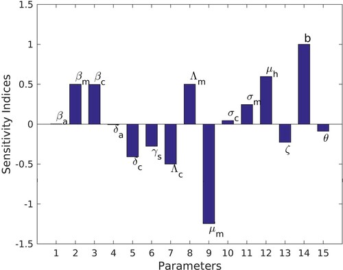
Table 3. Fitted parameter values for temperature function (16(16) $T(t)=T_0[1+T_1\cos ({\omega }_{1}t-{\psi }_1)],$(16) )

Parameter	$T_0$	$T_1$	${\psi }_1$	${\omega }_1$
Iringa	${26.7847}^{\mathrm{o}}$C	${0.0944}^{\mathrm{o}}$C	0.6681 Dimensionless	1.4167 month${}^{-1}$

Therefore, control strategies targeting the reduction of the biting rate ( through protecting individuals from mosquito bites) and increasing of mosquitoes' death rate (killing of the mosquitoes) will reduce transmission of malaria. Also, controlling the disease in children under five will have a high impact than controlling the disease in individuals aged five and above. The result is concurrent with that by Addawe and Lope [3] and Tchoumi et al. [28].

3. Model analysis with temperature dependent-parameters

This section incorporates the effect of temperature variability on malaria dynamics. The temperature-dependent parameters of the model 1(1) $\begin{array}{r}\begin{array}{ll}{\displaystyle \frac{\mathrm{d}{S}_c}{\mathrm{d}t}}& ={\mathrm{\Lambda }}_c+{\eta }_c{R}_c-({\mu }_h+{\lambda }_c(T)+\zeta )S_c,\\ {\displaystyle \frac{\mathrm{d}{E}_c}{\mathrm{d}t}}& ={\lambda }_c(T)S_c-({\mu }_h+{\sigma }_c+\zeta )E_c,\\ {\displaystyle \frac{\mathrm{d}{I}_c}{\mathrm{d}t}}& ={\sigma }_c{E}_c-({\mu }_h+{\delta }_c+\zeta +{\gamma }_c)I_c,\\ {\displaystyle \frac{\mathrm{d}{R}_c}{\mathrm{d}t}}& ={\gamma }_c{I}_c-(\zeta +{\mu }_h+{\eta }_c)R_c,\\ {\displaystyle \frac{\mathrm{d}{S}_a}{\mathrm{d}t}}& =\zeta S_c+{\eta }_a{R}_a-({\mu }_h+{\lambda }_a(T))S_a,\\ {\displaystyle \frac{\mathrm{d}{E}_a}{\mathrm{d}t}}& ={\lambda }_a(T)S_a+\zeta E_c-[{\mu }_h+{\sigma }_a\theta +(1-\theta ){\sigma }_a]E_a,\\ {\displaystyle \frac{\mathrm{d}{I}_a}{\mathrm{d}t}}& ={\sigma }_a\theta E_a+\zeta I_c-[{\mu }_h+{\delta }_a+{\gamma }_s]I_a,\\ {\displaystyle \frac{\mathrm{d}{A}_a}{\mathrm{d}t}}& ={\sigma }_a(1-\theta )E_a-({\mu }_h+{\gamma }_a)A_a,\\ {\displaystyle \frac{\mathrm{d}{R}_a}{\mathrm{d}t}}& ={\gamma }_a{A}_a+{\gamma }_s{I}_a+\zeta R_c-({\mu }_h+{\eta }_a)R_a,\\ {\displaystyle \frac{\mathrm{d}{S}_m}{\mathrm{d}t}}& ={\mathrm{\Lambda }}_m(T)-({\mu }_m(T)+{\lambda }_m(T))S_m,\\ {\displaystyle \frac{\mathrm{d}{E}_m}{\mathrm{d}t}}& ={\lambda }_m(T)S_m-({\mu }_m(T)+{\sigma }_m(T))E_m,\\ {\displaystyle \frac{\mathrm{d}{I}_m}{\mathrm{d}t}}& ={\sigma }_m(T)E_m-{\mu }_m(T)I_m,\end{array}\}\end{array}$(1) are defined as follows: The mosquito biting rate $b(T)$ [19] is defined as (11) $b(T)=-0.00014T^2+0.027T-0.322,$(11) Natural mortality rate for mosquito [19] is given by (12) ${\mu }_m(T)=-log(-0.000828T^2+0.0367T+0.522),$(12) and progression rate of mosquito [21] is (13) ${\sigma }_m(T)=\frac{T-Tmin}{DD},$(13) where $Tmin={16}^{\mathrm{o}}$C is the minimum temperature at which parasite development ceases and $DD={111}^{\mathrm{o}}\mathrm{C}\mathrm{days}$ is total degree days for the parasite development [25]. Recruitment of mosquito [19] is given by (14) ${\mathrm{\Lambda }}_m(T)=\frac{B(T)P_{EA}(T)}{{\tau }_{EA}(T)},$(14) where $B(T)$ is the lifetime number of eggs laid as given in [19], $EFD(T)$ is the number of eggs laid per female per day, $P_{EA}(T)$ is a probability that eggs survive to an adult mosquito and ${\tau }_{EA}(T)$ is the development time from egg to adult mosquito as in [5] (15) $\begin{array}{rl}B(T)& =\frac{EFD(T)}{{\mu }_m(T)},\\ EFD(T)& =-0.153T^2+8.61T-97.7,\\ P_{EA}(T)& =-0.000924T^2+0.453T-4.77,\\ {\tau }_{EA}(T)& =\frac{1}{-0.00094T^2+0.049T-0.552}.\end{array}$(15) Seasonal variation in temperature is modelled using the generalized function as in [25] given by (16) $T(t)=T_0[1+T_1\cos ({\omega }_{1}t-{\psi }_1)],$(16) where $T_0$ is the mean temperature in absence of seasonality, $T_1$ amplitude of seasonal variability in temperature, ${\omega }_1$ is frequency of seasonal oscillations in temperature and ${\psi }_1$ is the phase lag of temperature variability. The analyses of the temperature-dependent parameter model will be carried out using the data from the Iringa region in Tanzania.

3.1. Model fitting

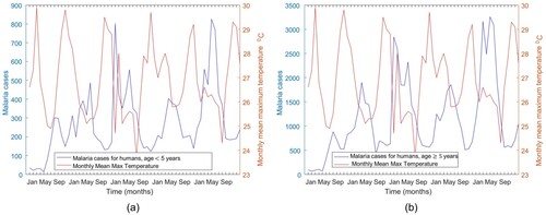
The temperature data used for this study was obtained from the Tanzania Meteorological Agency (TMA) through the author's personal correspondence. The data consists of the mean monthly maximum temperature (${}^{\mathrm{o}}$ C) for 2016 to 2020. Monthly Malaria cases for the same period were obtained from the Iringa referral hospital. Malaria cases are grouped into two groups. The first group represents malaria cases for humans under five years old, and the second group is for individuals aged five years and above. Figure 3 represents malaria cases and temperature data. Figure 3(a) shows malaria cases for humans under five and temperature and (b) shows malaria cases for humans aged five years and above and temperature.

Figure 3. Malaria cases and temperature data for Iringa region from 2016 to 2020.

3.1.1. Parameter estimates

According to the Tanzania National Bureau of Statistics (https://www.nbs.go.tz/index.php/en/), Iringa's life expectancy and total population in 2012 were 55.4 years and 941,238, respectively. Following the approach of [1], birth and death rate of human are estimated as follows:

Death rate (${\mu }_h$) (17) ${\mu }_h=\frac{1}{\mathrm{life}\mathrm{expectany}}=\frac{1}{55.4}\times \frac{1}{12}=0.001504\mathrm{per}\mathrm{month}.$(17) Human birth rate (${\mathrm{\Lambda }}_c$) (18) ${\mathrm{\Lambda }}_c={\mu }_h\times N_h=0.001504\times 941,238=1416\mathrm{human}\mathrm{per}\mathrm{monthy}.$(18) The temperature and malaria cases data presented in Figure 3 was used to calibrate the model parameters. The least-square fitting method in MATLAB programming language was used to fit the temperature variability function (16(16) $T(t)=T_0[1+T_1\cos ({\omega }_{1}t-{\psi }_1)],$(16) ) to the temperature data to obtain the parameter values in Table 3. Figure 4 shows the fitting of the function (16(16) $T(t)=T_0[1+T_1\cos ({\omega }_{1}t-{\psi }_1)],$(16) ).

Figure 4. Fitted curve for temperature from 2016 to 2020.

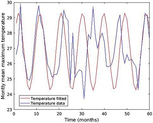
Figure 5. Cumulative malaria cases from the model fitted to real data for Iringa region from 2016 to 2018.

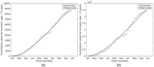
Table 6. Incremental cost-effectiveness ratios for optimal control strategies A, B, C, D, E, F and G.

Strategies	E	$\mathrm{\Delta }{E}_T$	C	$\mathrm{\Delta }{C}_T$	ICER
C	172,650,849	172,650,849	6,066,953.99	6,066,953.99	0.0351
B	172,706,986	56,137	6,067,738.64	784.65	0.0139
F	172,707,655	669	6,067,750.46	11.82	0.0177
A	172,735,692	28,037	29,578,264.19	23,510,513.73	838.5531
E	172,735,713	21	29,578,264.43	0.24	0.0114
D	172,748,667	12,954	29,578,410.03	145.60	0.0112
G	172,748,688	21	295,78410.28	0.25	0.0119

Using parameter values in Table 3 for the temperature functions (16(16) $T(t)=T_0[1+T_1\cos ({\omega }_{1}t-{\psi }_1)],$(16) ) together with temperature-dependent parameters in Equations (11(11) $b(T)=-0.00014T^2+0.027T-0.322,$(11) )–(15(15) $\begin{array}{rl}B(T)& =\frac{EFD(T)}{{\mu }_m(T)},\\ EFD(T)& =-0.153T^2+8.61T-97.7,\\ P_{EA}(T)& =-0.000924T^2+0.453T-4.77,\\ {\tau }_{EA}(T)& =\frac{1}{-0.00094T^2+0.049T-0.552}.\end{array}$(15) ), the model (1(1) $\begin{array}{r}\begin{array}{ll}{\displaystyle \frac{\mathrm{d}{S}_c}{\mathrm{d}t}}& ={\mathrm{\Lambda }}_c+{\eta }_c{R}_c-({\mu }_h+{\lambda }_c(T)+\zeta )S_c,\\ {\displaystyle \frac{\mathrm{d}{E}_c}{\mathrm{d}t}}& ={\lambda }_c(T)S_c-({\mu }_h+{\sigma }_c+\zeta )E_c,\\ {\displaystyle \frac{\mathrm{d}{I}_c}{\mathrm{d}t}}& ={\sigma }_c{E}_c-({\mu }_h+{\delta }_c+\zeta +{\gamma }_c)I_c,\\ {\displaystyle \frac{\mathrm{d}{R}_c}{\mathrm{d}t}}& ={\gamma }_c{I}_c-(\zeta +{\mu }_h+{\eta }_c)R_c,\\ {\displaystyle \frac{\mathrm{d}{S}_a}{\mathrm{d}t}}& =\zeta S_c+{\eta }_a{R}_a-({\mu }_h+{\lambda }_a(T))S_a,\\ {\displaystyle \frac{\mathrm{d}{E}_a}{\mathrm{d}t}}& ={\lambda }_a(T)S_a+\zeta E_c-[{\mu }_h+{\sigma }_a\theta +(1-\theta ){\sigma }_a]E_a,\\ {\displaystyle \frac{\mathrm{d}{I}_a}{\mathrm{d}t}}& ={\sigma }_a\theta E_a+\zeta I_c-[{\mu }_h+{\delta }_a+{\gamma }_s]I_a,\\ {\displaystyle \frac{\mathrm{d}{A}_a}{\mathrm{d}t}}& ={\sigma }_a(1-\theta )E_a-({\mu }_h+{\gamma }_a)A_a,\\ {\displaystyle \frac{\mathrm{d}{R}_a}{\mathrm{d}t}}& ={\gamma }_a{A}_a+{\gamma }_s{I}_a+\zeta R_c-({\mu }_h+{\eta }_a)R_a,\\ {\displaystyle \frac{\mathrm{d}{S}_m}{\mathrm{d}t}}& ={\mathrm{\Lambda }}_m(T)-({\mu }_m(T)+{\lambda }_m(T))S_m,\\ {\displaystyle \frac{\mathrm{d}{E}_m}{\mathrm{d}t}}& ={\lambda }_m(T)S_m-({\mu }_m(T)+{\sigma }_m(T))E_m,\\ {\displaystyle \frac{\mathrm{d}{I}_m}{\mathrm{d}t}}& ={\sigma }_m(T)E_m-{\mu }_m(T)I_m,\end{array}\}\end{array}$(1) ) was fitted to cumulative data on malaria cases per month from 2016 to 2018 for children under five and adults. The estimated parameter values are given in Table 4, and the fitted curve is shown in Figure 5.

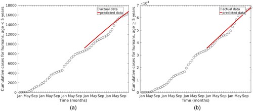
3.2. Model validation

To validate the model (1(1) $\begin{array}{r}\begin{array}{ll}{\displaystyle \frac{\mathrm{d}{S}_c}{\mathrm{d}t}}& ={\mathrm{\Lambda }}_c+{\eta }_c{R}_c-({\mu }_h+{\lambda }_c(T)+\zeta )S_c,\\ {\displaystyle \frac{\mathrm{d}{E}_c}{\mathrm{d}t}}& ={\lambda }_c(T)S_c-({\mu }_h+{\sigma }_c+\zeta )E_c,\\ {\displaystyle \frac{\mathrm{d}{I}_c}{\mathrm{d}t}}& ={\sigma }_c{E}_c-({\mu }_h+{\delta }_c+\zeta +{\gamma }_c)I_c,\\ {\displaystyle \frac{\mathrm{d}{R}_c}{\mathrm{d}t}}& ={\gamma }_c{I}_c-(\zeta +{\mu }_h+{\eta }_c)R_c,\\ {\displaystyle \frac{\mathrm{d}{S}_a}{\mathrm{d}t}}& =\zeta S_c+{\eta }_a{R}_a-({\mu }_h+{\lambda }_a(T))S_a,\\ {\displaystyle \frac{\mathrm{d}{E}_a}{\mathrm{d}t}}& ={\lambda }_a(T)S_a+\zeta E_c-[{\mu }_h+{\sigma }_a\theta +(1-\theta ){\sigma }_a]E_a,\\ {\displaystyle \frac{\mathrm{d}{I}_a}{\mathrm{d}t}}& ={\sigma }_a\theta E_a+\zeta I_c-[{\mu }_h+{\delta }_a+{\gamma }_s]I_a,\\ {\displaystyle \frac{\mathrm{d}{A}_a}{\mathrm{d}t}}& ={\sigma }_a(1-\theta )E_a-({\mu }_h+{\gamma }_a)A_a,\\ {\displaystyle \frac{\mathrm{d}{R}_a}{\mathrm{d}t}}& ={\gamma }_a{A}_a+{\gamma }_s{I}_a+\zeta R_c-({\mu }_h+{\eta }_a)R_a,\\ {\displaystyle \frac{\mathrm{d}{S}_m}{\mathrm{d}t}}& ={\mathrm{\Lambda }}_m(T)-({\mu }_m(T)+{\lambda }_m(T))S_m,\\ {\displaystyle \frac{\mathrm{d}{E}_m}{\mathrm{d}t}}& ={\lambda }_m(T)S_m-({\mu }_m(T)+{\sigma }_m(T))E_m,\\ {\displaystyle \frac{\mathrm{d}{I}_m}{\mathrm{d}t}}& ={\sigma }_m(T)E_m-{\mu }_m(T)I_m,\end{array}\}\end{array}$(1) ), parameter values in Table 4 were used. Figure 6 shows the simulated model using parameter values in Table 4 to predict the malaria cases data for 2019 to 2020.

Figure 6. Actual malaria cases from 2016 to 2020 and predicted cases from 2019 to 2020.

3.3. Effects of temperature variability on the malaria transmission dynamics

The model (1(1) $\begin{array}{r}\begin{array}{ll}{\displaystyle \frac{\mathrm{d}{S}_c}{\mathrm{d}t}}& ={\mathrm{\Lambda }}_c+{\eta }_c{R}_c-({\mu }_h+{\lambda }_c(T)+\zeta )S_c,\\ {\displaystyle \frac{\mathrm{d}{E}_c}{\mathrm{d}t}}& ={\lambda }_c(T)S_c-({\mu }_h+{\sigma }_c+\zeta )E_c,\\ {\displaystyle \frac{\mathrm{d}{I}_c}{\mathrm{d}t}}& ={\sigma }_c{E}_c-({\mu }_h+{\delta }_c+\zeta +{\gamma }_c)I_c,\\ {\displaystyle \frac{\mathrm{d}{R}_c}{\mathrm{d}t}}& ={\gamma }_c{I}_c-(\zeta +{\mu }_h+{\eta }_c)R_c,\\ {\displaystyle \frac{\mathrm{d}{S}_a}{\mathrm{d}t}}& =\zeta S_c+{\eta }_a{R}_a-({\mu }_h+{\lambda }_a(T))S_a,\\ {\displaystyle \frac{\mathrm{d}{E}_a}{\mathrm{d}t}}& ={\lambda }_a(T)S_a+\zeta E_c-[{\mu }_h+{\sigma }_a\theta +(1-\theta ){\sigma }_a]E_a,\\ {\displaystyle \frac{\mathrm{d}{I}_a}{\mathrm{d}t}}& ={\sigma }_a\theta E_a+\zeta I_c-[{\mu }_h+{\delta }_a+{\gamma }_s]I_a,\\ {\displaystyle \frac{\mathrm{d}{A}_a}{\mathrm{d}t}}& ={\sigma }_a(1-\theta )E_a-({\mu }_h+{\gamma }_a)A_a,\\ {\displaystyle \frac{\mathrm{d}{R}_a}{\mathrm{d}t}}& ={\gamma }_a{A}_a+{\gamma }_s{I}_a+\zeta R_c-({\mu }_h+{\eta }_a)R_a,\\ {\displaystyle \frac{\mathrm{d}{S}_m}{\mathrm{d}t}}& ={\mathrm{\Lambda }}_m(T)-({\mu }_m(T)+{\lambda }_m(T))S_m,\\ {\displaystyle \frac{\mathrm{d}{E}_m}{\mathrm{d}t}}& ={\lambda }_m(T)S_m-({\mu }_m(T)+{\sigma }_m(T))E_m,\\ {\displaystyle \frac{\mathrm{d}{I}_m}{\mathrm{d}t}}& ={\sigma }_m(T)E_m-{\mu }_m(T)I_m,\end{array}\}\end{array}$(1) ) is simulated with temperature variability using the fitted temperature function (16(16) $T(t)=T_0[1+T_1\cos ({\omega }_{1}t-{\psi }_1)],$(16) ). The mean temperature in the absence of seasonality is changed by increasing and reducing some degrees of temperature to have $T_0\pm [06{]}^{\mathrm{o}}$C. The aim is to investigate the effects of increased or decreased temperature on malaria transmission dynamics. The cumulative number of malaria cases for children under five and individuals aged five and above are presented in Figure 7.

Figure 7. Simulations showing the cumulative number of malaria cases in children under five and individuals aged five years and above when mean temperature in absence of seasonality is decreased by [0 6]${}^{\mathrm{o}}$C in (a) and (c), and when it is increased by [0 6]${}^{\mathrm{o}}$C in (b) and (d) respectively.

The results show that when the temperature $T_0$ in (16(16) $T(t)=T_0[1+T_1\cos ({\omega }_{1}t-{\psi }_1)],$(16) ) is increased, the cumulative malaria cases in children under five and individuals aged five and above is decreased as depicted in Figure 7(b ,d) respectively. Figure 7(a ,c) indicates an increase in cumulative malaria cases in children under five years and individuals aged five years and above when $T_0$ from (16(16) $T(t)=T_0[1+T_1\cos ({\omega }_{1}t-{\psi }_1)],$(16) ) is decreased by up to 2${}^{\mathrm{o}}$C. That means when the temperature in the absence of seasonality is in the range 24.78${}^{\mathrm{o}}$C to 26.78${}^{\mathrm{o}}$C, malaria cases are high, and below or above the range 24.78${}^{\mathrm{o}}$C to 26.78${}^{\mathrm{o}}$C cumulative malaria cases in human is decreased.

4. Temperature-dependent age-structured malaria model with optimal control

This section incorporates four-time dependent control strategies to control the spread of malaria. The control strategies considered are Long Lasting Insecticide Nets (LLINs) to protect individuals from mosquito bites, treatment of symptomatic (under five $I_c$ and five and above years human $I_a$), screening and treatment of asymptomatic carrier $(A_a)$ and mosquito adulticide efforts (spray of insecticide). The aim is to minimize the number of infected humans (under five and above five years) and mosquito populations and the costs of applying them. The system (1(1) $\begin{array}{r}\begin{array}{ll}{\displaystyle \frac{\mathrm{d}{S}_c}{\mathrm{d}t}}& ={\mathrm{\Lambda }}_c+{\eta }_c{R}_c-({\mu }_h+{\lambda }_c(T)+\zeta )S_c,\\ {\displaystyle \frac{\mathrm{d}{E}_c}{\mathrm{d}t}}& ={\lambda }_c(T)S_c-({\mu }_h+{\sigma }_c+\zeta )E_c,\\ {\displaystyle \frac{\mathrm{d}{I}_c}{\mathrm{d}t}}& ={\sigma }_c{E}_c-({\mu }_h+{\delta }_c+\zeta +{\gamma }_c)I_c,\\ {\displaystyle \frac{\mathrm{d}{R}_c}{\mathrm{d}t}}& ={\gamma }_c{I}_c-(\zeta +{\mu }_h+{\eta }_c)R_c,\\ {\displaystyle \frac{\mathrm{d}{S}_a}{\mathrm{d}t}}& =\zeta S_c+{\eta }_a{R}_a-({\mu }_h+{\lambda }_a(T))S_a,\\ {\displaystyle \frac{\mathrm{d}{E}_a}{\mathrm{d}t}}& ={\lambda }_a(T)S_a+\zeta E_c-[{\mu }_h+{\sigma }_a\theta +(1-\theta ){\sigma }_a]E_a,\\ {\displaystyle \frac{\mathrm{d}{I}_a}{\mathrm{d}t}}& ={\sigma }_a\theta E_a+\zeta I_c-[{\mu }_h+{\delta }_a+{\gamma }_s]I_a,\\ {\displaystyle \frac{\mathrm{d}{A}_a}{\mathrm{d}t}}& ={\sigma }_a(1-\theta )E_a-({\mu }_h+{\gamma }_a)A_a,\\ {\displaystyle \frac{\mathrm{d}{R}_a}{\mathrm{d}t}}& ={\gamma }_a{A}_a+{\gamma }_s{I}_a+\zeta R_c-({\mu }_h+{\eta }_a)R_a,\\ {\displaystyle \frac{\mathrm{d}{S}_m}{\mathrm{d}t}}& ={\mathrm{\Lambda }}_m(T)-({\mu }_m(T)+{\lambda }_m(T))S_m,\\ {\displaystyle \frac{\mathrm{d}{E}_m}{\mathrm{d}t}}& ={\lambda }_m(T)S_m-({\mu }_m(T)+{\sigma }_m(T))E_m,\\ {\displaystyle \frac{\mathrm{d}{I}_m}{\mathrm{d}t}}& ={\sigma }_m(T)E_m-{\mu }_m(T)I_m,\end{array}\}\end{array}$(1) ) is then modified to obtain an optimal control problem given in the following system of equations (19) $\begin{array}{r}\begin{array}{ll}{\displaystyle {\displaystyle \frac{\mathrm{d}{S}_c}{\mathrm{d}t}}}& ={\mathrm{\Lambda }}_c+{\eta }_c{R}_c-(1-w_c{u}_1){\lambda }_c(T)S_c-({\mu }_h+\zeta )S_c,\\ {\displaystyle {\displaystyle \frac{\mathrm{d}{E}_c}{\mathrm{d}t}}}& =(1-w_c{u}_1){\lambda }_c(T)S_c-({\mu }_h+{\sigma }_c+\zeta )E_c,\\ {\displaystyle {\displaystyle \frac{\mathrm{d}{I}_c}{\mathrm{d}t}}}& ={\sigma }_c{E}_c-({\mu }_h+{\delta }_c+\zeta +{\gamma }_c+u_2\tau )I_c,\\ {\displaystyle {\displaystyle \frac{\mathrm{d}{R}_c}{\mathrm{d}t}}}& =({\gamma }_c+u_2\tau )I_c-(\zeta +{\mu }_h+{\eta }_c)R_c,\\ {\displaystyle {\displaystyle \frac{\mathrm{d}{S}_a}{\mathrm{d}t}}}& =\zeta S_c+{\eta }_a{R}_a-({\mu }_h+(1-w_a{u}_1){\lambda }_a(T))S_a,\\ {\displaystyle {\displaystyle \frac{\mathrm{d}{E}_a}{\mathrm{d}t}}}& =(1-w_a{u}_1){\lambda }_a(T)S_a+\zeta E_c-[{\mu }_h+{\sigma }_a\theta +(1-\theta ){\sigma }_a]E_a,\\ {\displaystyle {\displaystyle \frac{\mathrm{d}{I}_a}{\mathrm{d}t}}}& ={\sigma }_a\theta E_a+\zeta I_c-[{\mu }_h+{\delta }_a+({\gamma }_s+u_2\tau )]I_a,\\ {\displaystyle {\displaystyle \frac{\mathrm{d}{A}_a}{\mathrm{d}t}}}& ={\sigma }_a(1-\theta )E_a-({\mu }_h+{\gamma }_a+u_3\tau )A_a,\\ {\displaystyle {\displaystyle \frac{\mathrm{d}{R}_a}{\mathrm{d}t}}}& =({\gamma }_a+u_3\tau )A_a+({\gamma }_s+u_2\tau )I_a+\zeta R_c-({\mu }_h+{\eta }_a)R_a,\\ {\displaystyle {\displaystyle \frac{\mathrm{d}{S}_m}{\mathrm{d}t}}}& ={\mathrm{\Lambda }}_m(T)-{\lambda }_m(T)S_m-({\mu }_m(T)+w_m{u}_4)S_m,\\ {\displaystyle {\displaystyle \frac{\mathrm{d}{E}_m}{\mathrm{d}t}}}& ={\lambda }_m(T)S_m-({\sigma }_m+{\mu }_m(T)+w_m{u}_4)E_m,\\ {\displaystyle {\displaystyle \frac{\mathrm{d}{I}_m}{\mathrm{d}t}}}& ={\sigma }_m{E}_m-({\mu }_m(T)+w_m{u}_4)I_m,\end{array}\}\end{array}$(19) with ${\lambda }_c$ and ${\lambda }_a$ as defined in system 1(1) $\begin{array}{r}\begin{array}{ll}{\displaystyle \frac{\mathrm{d}{S}_c}{\mathrm{d}t}}& ={\mathrm{\Lambda }}_c+{\eta }_c{R}_c-({\mu }_h+{\lambda }_c(T)+\zeta )S_c,\\ {\displaystyle \frac{\mathrm{d}{E}_c}{\mathrm{d}t}}& ={\lambda }_c(T)S_c-({\mu }_h+{\sigma }_c+\zeta )E_c,\\ {\displaystyle \frac{\mathrm{d}{I}_c}{\mathrm{d}t}}& ={\sigma }_c{E}_c-({\mu }_h+{\delta }_c+\zeta +{\gamma }_c)I_c,\\ {\displaystyle \frac{\mathrm{d}{R}_c}{\mathrm{d}t}}& ={\gamma }_c{I}_c-(\zeta +{\mu }_h+{\eta }_c)R_c,\\ {\displaystyle \frac{\mathrm{d}{S}_a}{\mathrm{d}t}}& =\zeta S_c+{\eta }_a{R}_a-({\mu }_h+{\lambda }_a(T))S_a,\\ {\displaystyle \frac{\mathrm{d}{E}_a}{\mathrm{d}t}}& ={\lambda }_a(T)S_a+\zeta E_c-[{\mu }_h+{\sigma }_a\theta +(1-\theta ){\sigma }_a]E_a,\\ {\displaystyle \frac{\mathrm{d}{I}_a}{\mathrm{d}t}}& ={\sigma }_a\theta E_a+\zeta I_c-[{\mu }_h+{\delta }_a+{\gamma }_s]I_a,\\ {\displaystyle \frac{\mathrm{d}{A}_a}{\mathrm{d}t}}& ={\sigma }_a(1-\theta )E_a-({\mu }_h+{\gamma }_a)A_a,\\ {\displaystyle \frac{\mathrm{d}{R}_a}{\mathrm{d}t}}& ={\gamma }_a{A}_a+{\gamma }_s{I}_a+\zeta R_c-({\mu }_h+{\eta }_a)R_a,\\ {\displaystyle \frac{\mathrm{d}{S}_m}{\mathrm{d}t}}& ={\mathrm{\Lambda }}_m(T)-({\mu }_m(T)+{\lambda }_m(T))S_m,\\ {\displaystyle \frac{\mathrm{d}{E}_m}{\mathrm{d}t}}& ={\lambda }_m(T)S_m-({\mu }_m(T)+{\sigma }_m(T))E_m,\\ {\displaystyle \frac{\mathrm{d}{I}_m}{\mathrm{d}t}}& ={\sigma }_m(T)E_m-{\mu }_m(T)I_m,\end{array}\}\end{array}$(1) , but ${\lambda }_m=\frac{b{\beta }_m[(1-w_c{u}_1)I_c+(1-w_a{u}_1)I_a+r(1-w_a{u}_1)A_a]}{N_h}$. $u_1(t)\in [0,1]$ is the time-dependent control effort for the use of LLINs that protect individuals from mosquito bites, w is the measure of the effectiveness of LLINs in protecting under five $(w_c)$ and five and above years $(w_a)$. $u_2(t)\tau$ is a recovered rate after treatment, $u_2(t)\in [0,1]$ is the time-dependent treatment effort of symptomatic individuals ($I_c$, $I_a$) with drug efficacy τ. ${\gamma }_a+u_2(t)\tau$ is a clearance rate for asymptomatic individuals, ${\gamma }_a$ is a natural recovered rate and $u_3(t)\in [0,1]$ is the time-dependent control for screening and treating asymptomatic individuals with drug efficacy τ. $u_4(t)\in [0,1]$ is the mosquito adulticide effort using insecticide spraying with killing efficacy $w_m$. The objective function is defined as (20) $J(u_1,u_2,u_3,u_4)={\int }_0^{t_f}(A_1{I}_c+A_2{I}_a+A_3{A}_a+B_1{S}_m+B_2{E}_m+B_3{I}_m+P)\mathrm{d}t$(20) where $P=\sum _{i=1}^5\frac{C_i{u}_i^2(t)}{2}$, the coefficients $A_1$, $A_2$, $A_3$, $B_1$,$B_2$, $B_3$ are weights for infectious under five ($I_c$), five and above symptomatic individuals ($I_a$), asymptomatic carriers ($A_a$), susceptible($S_m$), exposed ($E_m$) and infectious ($I_m$) mosquitoes respectively. All mosquito populations are included in an objective function because insecticide affects all mosquitoes. $C_i$, i = 1, 2, 3, 4 are cost balancing factors for control over time $t\in [0,t_f]$. $\frac{C_1{u}_1^2}{2}$, $\frac{C_2{u}_2^2}{2}$, $\frac{C_3{u}_3^2}{2}$ and $\frac{C_4{u}_4^2}{2}$ represents the cost of control efforts needed for personal protection using LLINs, treatment of symptomatic infectious individuals ($I_c$ and $I_a$) and screening and treatment of asymptomatic carrier. Quadratic cost on controls is used as in [4,13,17] since the cost associated with control is non-linear. The aim is to minimize the objective functional J, to do so optimal control $u_1^{\ast }$, $u_2^{\ast }$, $u_3^{\ast }$, $u_4^{\ast }$ are determined, such that $J(u_1^{\ast },u_2^{\ast },u_3^{\ast },u_4^{\ast })=min\{J(u_1,u_2,u_3,u_4)\}.$The necessary conditions an optimal system must satisfy are derived from Pontryagin's Maximum principle. The principle converts (19(19) $\begin{array}{r}\begin{array}{ll}{\displaystyle {\displaystyle \frac{\mathrm{d}{S}_c}{\mathrm{d}t}}}& ={\mathrm{\Lambda }}_c+{\eta }_c{R}_c-(1-w_c{u}_1){\lambda }_c(T)S_c-({\mu }_h+\zeta )S_c,\\ {\displaystyle {\displaystyle \frac{\mathrm{d}{E}_c}{\mathrm{d}t}}}& =(1-w_c{u}_1){\lambda }_c(T)S_c-({\mu }_h+{\sigma }_c+\zeta )E_c,\\ {\displaystyle {\displaystyle \frac{\mathrm{d}{I}_c}{\mathrm{d}t}}}& ={\sigma }_c{E}_c-({\mu }_h+{\delta }_c+\zeta +{\gamma }_c+u_2\tau )I_c,\\ {\displaystyle {\displaystyle \frac{\mathrm{d}{R}_c}{\mathrm{d}t}}}& =({\gamma }_c+u_2\tau )I_c-(\zeta +{\mu }_h+{\eta }_c)R_c,\\ {\displaystyle {\displaystyle \frac{\mathrm{d}{S}_a}{\mathrm{d}t}}}& =\zeta S_c+{\eta }_a{R}_a-({\mu }_h+(1-w_a{u}_1){\lambda }_a(T))S_a,\\ {\displaystyle {\displaystyle \frac{\mathrm{d}{E}_a}{\mathrm{d}t}}}& =(1-w_a{u}_1){\lambda }_a(T)S_a+\zeta E_c-[{\mu }_h+{\sigma }_a\theta +(1-\theta ){\sigma }_a]E_a,\\ {\displaystyle {\displaystyle \frac{\mathrm{d}{I}_a}{\mathrm{d}t}}}& ={\sigma }_a\theta E_a+\zeta I_c-[{\mu }_h+{\delta }_a+({\gamma }_s+u_2\tau )]I_a,\\ {\displaystyle {\displaystyle \frac{\mathrm{d}{A}_a}{\mathrm{d}t}}}& ={\sigma }_a(1-\theta )E_a-({\mu }_h+{\gamma }_a+u_3\tau )A_a,\\ {\displaystyle {\displaystyle \frac{\mathrm{d}{R}_a}{\mathrm{d}t}}}& =({\gamma }_a+u_3\tau )A_a+({\gamma }_s+u_2\tau )I_a+\zeta R_c-({\mu }_h+{\eta }_a)R_a,\\ {\displaystyle {\displaystyle \frac{\mathrm{d}{S}_m}{\mathrm{d}t}}}& ={\mathrm{\Lambda }}_m(T)-{\lambda }_m(T)S_m-({\mu }_m(T)+w_m{u}_4)S_m,\\ {\displaystyle {\displaystyle \frac{\mathrm{d}{E}_m}{\mathrm{d}t}}}& ={\lambda }_m(T)S_m-({\sigma }_m+{\mu }_m(T)+w_m{u}_4)E_m,\\ {\displaystyle {\displaystyle \frac{\mathrm{d}{I}_m}{\mathrm{d}t}}}& ={\sigma }_m{E}_m-({\mu }_m(T)+w_m{u}_4)I_m,\end{array}\}\end{array}$(19) ) and (20(20) $J(u_1,u_2,u_3,u_4)={\int }_0^{t_f}(A_1{I}_c+A_2{I}_a+A_3{A}_a+B_1{S}_m+B_2{E}_m+B_3{I}_m+P)\mathrm{d}t$(20) ) into the problem of minimizing point-wise Hamiltonian H with respect to $u_1$, $u_2$, $u_3$, $u_4$ as (21) $\begin{array}{rl}H& =A_1{I}_c+A_2{I}_a+A_3{A}_a+B_1{S}_m+B_2{E}_m+B_3{I}_m+{\lambda }_{S_c}\frac{\mathrm{d}{S}_c}{\mathrm{d}t}+{\lambda }_{E_c}\frac{\mathrm{d}{E}_c}{\mathrm{d}t}\\ & +{\lambda }_{I_c}\frac{\mathrm{d}{I}_c}{\mathrm{d}t}+{\lambda }_{R_c}\frac{d{R}_c}{\mathrm{d}t}+{\lambda }_{S_a}\frac{\mathrm{d}{S}_a}{\mathrm{d}t}+{\lambda }_{E_a}\frac{\mathrm{d}{E}_a}{\mathrm{d}t}+{\lambda }_{I_a}\frac{\mathrm{d}{I}_a}{\mathrm{d}t}+{\lambda }_{A_a}\frac{\mathrm{d}{A}_a}{\mathrm{d}t}+{\lambda }_{R_a}\frac{d{R}_a}{\mathrm{d}t}\\ & +{\lambda }_{S_m}\frac{\mathrm{d}{S}_m}{\mathrm{d}t}+{\lambda }_{E_m}\frac{d{E}_m}{\mathrm{d}t}+{\lambda }_{I_m}\frac{\mathrm{d}{I}_m}{\mathrm{d}t}.\end{array}$(21) Substituting the equations of the system of the optimal control problem (19(19) $\begin{array}{r}\begin{array}{ll}{\displaystyle {\displaystyle \frac{\mathrm{d}{S}_c}{\mathrm{d}t}}}& ={\mathrm{\Lambda }}_c+{\eta }_c{R}_c-(1-w_c{u}_1){\lambda }_c(T)S_c-({\mu }_h+\zeta )S_c,\\ {\displaystyle {\displaystyle \frac{\mathrm{d}{E}_c}{\mathrm{d}t}}}& =(1-w_c{u}_1){\lambda }_c(T)S_c-({\mu }_h+{\sigma }_c+\zeta )E_c,\\ {\displaystyle {\displaystyle \frac{\mathrm{d}{I}_c}{\mathrm{d}t}}}& ={\sigma }_c{E}_c-({\mu }_h+{\delta }_c+\zeta +{\gamma }_c+u_2\tau )I_c,\\ {\displaystyle {\displaystyle \frac{\mathrm{d}{R}_c}{\mathrm{d}t}}}& =({\gamma }_c+u_2\tau )I_c-(\zeta +{\mu }_h+{\eta }_c)R_c,\\ {\displaystyle {\displaystyle \frac{\mathrm{d}{S}_a}{\mathrm{d}t}}}& =\zeta S_c+{\eta }_a{R}_a-({\mu }_h+(1-w_a{u}_1){\lambda }_a(T))S_a,\\ {\displaystyle {\displaystyle \frac{\mathrm{d}{E}_a}{\mathrm{d}t}}}& =(1-w_a{u}_1){\lambda }_a(T)S_a+\zeta E_c-[{\mu }_h+{\sigma }_a\theta +(1-\theta ){\sigma }_a]E_a,\\ {\displaystyle {\displaystyle \frac{\mathrm{d}{I}_a}{\mathrm{d}t}}}& ={\sigma }_a\theta E_a+\zeta I_c-[{\mu }_h+{\delta }_a+({\gamma }_s+u_2\tau )]I_a,\\ {\displaystyle {\displaystyle \frac{\mathrm{d}{A}_a}{\mathrm{d}t}}}& ={\sigma }_a(1-\theta )E_a-({\mu }_h+{\gamma }_a+u_3\tau )A_a,\\ {\displaystyle {\displaystyle \frac{\mathrm{d}{R}_a}{\mathrm{d}t}}}& =({\gamma }_a+u_3\tau )A_a+({\gamma }_s+u_2\tau )I_a+\zeta R_c-({\mu }_h+{\eta }_a)R_a,\\ {\displaystyle {\displaystyle \frac{\mathrm{d}{S}_m}{\mathrm{d}t}}}& ={\mathrm{\Lambda }}_m(T)-{\lambda }_m(T)S_m-({\mu }_m(T)+w_m{u}_4)S_m,\\ {\displaystyle {\displaystyle \frac{\mathrm{d}{E}_m}{\mathrm{d}t}}}& ={\lambda }_m(T)S_m-({\sigma }_m+{\mu }_m(T)+w_m{u}_4)E_m,\\ {\displaystyle {\displaystyle \frac{\mathrm{d}{I}_m}{\mathrm{d}t}}}& ={\sigma }_m{E}_m-({\mu }_m(T)+w_m{u}_4)I_m,\end{array}\}\end{array}$(19) ) into (21(21) $\begin{array}{rl}H& =A_1{I}_c+A_2{I}_a+A_3{A}_a+B_1{S}_m+B_2{E}_m+B_3{I}_m+{\lambda }_{S_c}\frac{\mathrm{d}{S}_c}{\mathrm{d}t}+{\lambda }_{E_c}\frac{\mathrm{d}{E}_c}{\mathrm{d}t}\\ & +{\lambda }_{I_c}\frac{\mathrm{d}{I}_c}{\mathrm{d}t}+{\lambda }_{R_c}\frac{d{R}_c}{\mathrm{d}t}+{\lambda }_{S_a}\frac{\mathrm{d}{S}_a}{\mathrm{d}t}+{\lambda }_{E_a}\frac{\mathrm{d}{E}_a}{\mathrm{d}t}+{\lambda }_{I_a}\frac{\mathrm{d}{I}_a}{\mathrm{d}t}+{\lambda }_{A_a}\frac{\mathrm{d}{A}_a}{\mathrm{d}t}+{\lambda }_{R_a}\frac{d{R}_a}{\mathrm{d}t}\\ & +{\lambda }_{S_m}\frac{\mathrm{d}{S}_m}{\mathrm{d}t}+{\lambda }_{E_m}\frac{d{E}_m}{\mathrm{d}t}+{\lambda }_{I_m}\frac{\mathrm{d}{I}_m}{\mathrm{d}t}.\end{array}$(21) ) gives (22) $\begin{array}{rl}H& =A_1{I}_c+A_2{I}_a+A_3{A}_a+B_1{S}_m+B_2{E}_m+B_3{I}_m\\ & +{\lambda }_{S_c}[{\mathrm{\Lambda }}_c+{\eta }_c{R}_c-(1-w_c{u}_1){\lambda }_c(T)S_c-({\mu }_h+\zeta )S_c]\\ & +{\lambda }_{E_c}[(1-w_c{u}_1){\lambda }_c(T)S_c-({\mu }_h+{\sigma }_c+\zeta )E_c]\\ & +{\lambda }_{I_c}[{\sigma }_c{E}_c-({\mu }_h+{\delta }_c+\zeta +{\gamma }_c+u_2\tau )I_c]\\ & +{\lambda }_{R_c}[({\gamma }_c+u_2\tau )I_c-(\zeta +{\mu }_h+{\eta }_c)R_c]\\ & +{\lambda }_{S_a}[\zeta S_c+{\eta }_a{R}_a]\\ & -{\lambda }_{S_a}[({\mu }_h+(1-w_a{u}_1){\lambda }_a(T))S_a]\\ & +{\lambda }_{E_a}[(1-w_a{u}_1){\lambda }_a(T)S_a+\zeta E_c]\\ & -{\lambda }_{E_a}\left[[{\mu }_h+{\sigma }_a\theta +(1-\theta ){\sigma }_a]E_a\right]\\ & +{\lambda }_{I_a}[{\sigma }_a\theta E_a+\zeta I_c-[{\mu }_h+{\delta }_a+({\gamma }_s+u_2\tau )]I_a]\\ & +{\lambda }_{A_a}[{\sigma }_a(1-\theta )E_a{I}_a-({\mu }_h+{\gamma }_a+u_3\tau )A_a]\\ & +{\lambda }_{R_a}[({\gamma }_a+u_3\tau )A_a+({\gamma }_s+u_2\tau )I_a+\zeta R_c-({\mu }_h+{\eta }_a)R_a]\\ & +{\lambda }_{S_m}[{\mathrm{\Lambda }}_m(T)-{\lambda }_m(T)S_m-({\mu }_m(T)+w_m{u}_4)S_m]\\ & +{\lambda }_{E_m}[{\lambda }_m(T)S_m-({\sigma }_m+{\mu }_m(T)+w_m{u}_4)E_m]\\ & +{\lambda }_{I_m}[{\sigma }_m{E}_m-({\mu }_m(T)+w_m{u}_4)I_m].\end{array}$(22) where ${\lambda }_{S_c}$, ${\lambda }_{E_c}$, ${\lambda }_{I_c}$, ${\lambda }_{R_c}$, ${\lambda }_{S_a}$, ${\lambda }_{E_a}$, ${\lambda }_{I_a}$, ${\lambda }_{A_a}$, ${\lambda }_{R_a}$, ${\lambda }_{S_m}$, ${\lambda }_{E_m}$ and ${\lambda }_{I_m}$ are adjoint variables. The adjoint equation is then given by (23) $\begin{array}{rl}\frac{\mathrm{d}{\lambda }_{S_c}}{\mathrm{d}t}& =-{\lambda }_{S_a}\zeta -{\lambda }_{S_c}(-\zeta -{\mu }_h-\frac{I_{m}b(1-u_1{w}_c){\beta }_c}{N_h})-\frac{{\lambda }_{E_c}{I}_{m}b(1-u_1{w}_c){\beta }_c}{N_h},\\ \frac{\mathrm{d}{\lambda }_{E_c}}{\mathrm{d}t}& =-{\lambda }_{I_c}{\sigma }_c-{\lambda }_{E_c}(-{\sigma }_c-\zeta -{\mu }_h)-{\lambda }_{E_a}\zeta ,\\ \frac{\mathrm{d}{\lambda }_{I_c}}{\mathrm{d}t}& =-{\lambda }_{I_c}(-u_2\tau -\zeta -{\mu }_h-{\delta }_c-{\gamma }_c)-{\lambda }_{R_c}{u}_2\tau -{\lambda }_{I_a}\zeta -\frac{\mathrm{d}{\lambda }_{E_m}{S}_{m}b(1-u_1{w}_c){\beta }_m}{N_h}\\ & -\frac{{\lambda }_{S_m}{S}_{m}b(1-u_1{w}_c){\beta }_m}{N_h}-A_1,\\ \frac{\mathrm{d}{\lambda }_{R_c}}{\mathrm{d}t}& =-{\lambda }_{R_a}\zeta -{\lambda }_{R_c}(-\zeta -{\mu }_h-{\eta }_c)-{\lambda }_{S_c}{\eta }_c,\\ \frac{\mathrm{d}{\lambda }_{S_a}}{\mathrm{d}t}& =-{\lambda }_{S_a}(-{\mu }_h-\frac{I_{m}b(1-u_1{w}_a){\beta }_a}{N_h})-\frac{\mathrm{d}{\lambda }_{E_a}{I}_{m}b(1-u_1{w}_a){\beta }_a}{N_h},\\ \frac{\mathrm{d}{\lambda }_{E_a}}{\mathrm{d}t}& =-{\lambda }_{I_a}\theta {\sigma }_a-{\lambda }_{A_a}(1-\theta ){\sigma }_a-{\lambda }_{E_a}(-{\sigma }_a-{\mu }_h),\\ \frac{\mathrm{d}{\lambda }_{I_a}}{\mathrm{d}t}& =-{\lambda }_{I_a}((-u_2\tau -{\gamma }_s)-{\mu }_h-{\delta }_a)-{\lambda }_{R_a}(u_2\tau +{\gamma }_s)-\frac{{\lambda }_{E_m}{S}_{m}b(1-u_1{w}_a){\beta }_m}{N_h}\\ & -\frac{{\lambda }_{S_m}{S}_{m}b(1-u_1{w}_a){\beta }_m}{N_h}-A_2,\\ \frac{\mathrm{d}{\lambda }_{A_a}}{\mathrm{d}t}& =-{\lambda }_{R_a}(u_3\tau +{\gamma }_a)-{\lambda }_{A_a}(-u_3\tau -{\mu }_h-{\gamma }_a)-\frac{{\lambda }_{E_m}{S}_{m}br(1-u_1{w}_a){\beta }_m}{N_h}\\ & -\frac{{\lambda }_{S_m}{S}_{m}br(1-u_1{w}_a){\beta }_m}{N_h}-A_3,\\ \frac{\mathrm{d}{\lambda }_{R_a}}{\mathrm{d}t}& =-{\lambda }_{R_a}(-{\mu }_h-{\eta }_a)-{\lambda }_{S_a}{\eta }_a,\\ \frac{\mathrm{d}{\lambda }_{S_m}}{\mathrm{d}t}& =-{\lambda }_{S_m}(\frac{b(I_c(1-u_1{w}_c)+A_{a}r(1-u_1{w}_a)+I_a(1-u_1{w}_a)){\beta }_m}{N_h}-{\mu }_m)\\ & -\frac{{\lambda }_{E_m}{I}_{c}b(1-u_1{w}_c){\beta }_m}{N_h}-\frac{{\lambda }_{E_m}b(A_{a}r(1-u_1{w}_a)+I_a(1-u_1{w}_a)){\beta }_m}{N_h}-B_1,\\ \frac{\mathrm{d}{\lambda }_{E_m}}{\mathrm{d}t}& =-{\lambda }_{I_m}{\sigma }_m+{\lambda }_{E_m}{\lambda }_{A_a}-B_2,\\ \frac{\mathrm{d}{\lambda }_{I_m}}{\mathrm{d}t}& =-{\lambda }_{I_m}(-{\mu }_m-u_4{w}_m)-\frac{{\lambda }_{E_c}{S}_{c}b(1-u_1{w}_c){\beta }_c}{N_h}+\frac{{\lambda }_{S_c}{S}_{c}b(1-u_1{w}_c){\beta }_c}{N_h}\\ & -\frac{{\lambda }_{E_a}{S}_{a}b(1-u_1{w}_a){\beta }_a}{N_h}+\frac{{\lambda }_{S_a}{S}_{a}b(1-u_1{w}_a){\beta }_a}{N_h}-B_3,\end{array}$(23) with transversality conditions ${\lambda }_{S_c}(t_f)={\lambda }_{E_c}(t_f)={\lambda }_{I_c}(t_f)={\lambda }_{R_c}(t_f)={\lambda }_{S_a}(t_f)={\lambda }_{E_a}(t_f)={\lambda }_{I_a}(t_f)={\lambda }_{A_a}(t_f)={\lambda }_{R_a}(t_f)={\lambda }_{S_m}(t_f)={\lambda }_{E_m}(t_f)={\lambda }_{I_m}(t_f)=0$ and $\frac{\mathrm{\partial }H}{\mathrm{\partial }{u}_i}=0$ at $u_i=0$, i = 1, 2, 3, 4 optimal conditions. Then (24) $\begin{array}{rl}\frac{\mathrm{\partial }H}{\mathrm{\partial }{u}_1}& =\frac{{\lambda }_{E_m}{S}_{m}b(-I_c{w}_c-A_{a}r{w}_a-I_a{w}_a){\beta }_m}{N_h}+\frac{{\lambda }_{S_m}{S}_{m}b(-I_c{w}_c-A_{a}r{w}_a-I_a{w}_a){\beta }_m}{N_h}\\ & -\frac{{\lambda }_{E_c}{I}_m{S}_{c}b{w}_c{\beta }_c}{N_h}+\frac{{\lambda }_{S_c}{I}_m{S}_{c}b{w}_c{\beta }_c}{N_h}\\ & -\frac{{\lambda }_{E_a}{I}_m{S}_{a}b{w}_a{\beta }_a}{N_h}+\frac{{\lambda }_{S_a}{I}_m{S}_{a}b{w}_a{\beta }_a}{N_h}+C_1{u}_1=0,\\ \frac{\mathrm{\partial }H}{\mathrm{\partial }{u}_2}& =-{\lambda }_{I_a}{I}_a\tau +{\lambda }_{R_a}{I}_a\tau +{\lambda }_{R_c}{I}_c\tau -{\lambda }_{I_c}{I}_c\tau +C_2{u}_2=0,\\ \frac{\mathrm{\partial }H}{\mathrm{\partial }{u}_3}& =A_a{\lambda }_{R_a}\tau -A_a{\lambda }_{A_a}\tau +C_3{u}_3=0,\\ \frac{\mathrm{\partial }H}{\mathrm{\partial }{u}_4}& =C_4{u}_4-{\lambda }_{I_m}{I}_m{w}_m=0.\end{array}$(24) Solving (24(24) $\begin{array}{rl}\frac{\mathrm{\partial }H}{\mathrm{\partial }{u}_1}& =\frac{{\lambda }_{E_m}{S}_{m}b(-I_c{w}_c-A_{a}r{w}_a-I_a{w}_a){\beta }_m}{N_h}+\frac{{\lambda }_{S_m}{S}_{m}b(-I_c{w}_c-A_{a}r{w}_a-I_a{w}_a){\beta }_m}{N_h}\\ & -\frac{{\lambda }_{E_c}{I}_m{S}_{c}b{w}_c{\beta }_c}{N_h}+\frac{{\lambda }_{S_c}{I}_m{S}_{c}b{w}_c{\beta }_c}{N_h}\\ & -\frac{{\lambda }_{E_a}{I}_m{S}_{a}b{w}_a{\beta }_a}{N_h}+\frac{{\lambda }_{S_a}{I}_m{S}_{a}b{w}_a{\beta }_a}{N_h}+C_1{u}_1=0,\\ \frac{\mathrm{\partial }H}{\mathrm{\partial }{u}_2}& =-{\lambda }_{I_a}{I}_a\tau +{\lambda }_{R_a}{I}_a\tau +{\lambda }_{R_c}{I}_c\tau -{\lambda }_{I_c}{I}_c\tau +C_2{u}_2=0,\\ \frac{\mathrm{\partial }H}{\mathrm{\partial }{u}_3}& =A_a{\lambda }_{R_a}\tau -A_a{\lambda }_{A_a}\tau +C_3{u}_3=0,\\ \frac{\mathrm{\partial }H}{\mathrm{\partial }{u}_4}& =C_4{u}_4-{\lambda }_{I_m}{I}_m{w}_m=0.\end{array}$(24) ) for $u_i$ gives (25) $\begin{array}{rl}{u}_1& =\frac{(({\lambda }_{E_m}+{\lambda }_{S_m})I_c{S}_{m}b{w}_c+(A_a{\lambda }_{E_m}+A_a{\lambda }_{S_m})S_{m}br{w}_a){\beta }_m}{C_1{N}_h}\\ & +\frac{({\lambda }_{E_m}+{\lambda }_{S_m})I_a{S}_{m}b{w}_a{\beta }_m}{C_1{N}_h}\\ & +\frac{({\lambda }_{E_c}-{\lambda }_{S_c})I_m{S}_{c}b{w}_c{\beta }_c+({\lambda }_{E_a}-{\lambda }_{S_a})I_m{S}_{a}b{w}_a{\beta }_a}{C_1{N}_h},\\ u_2& =-\frac{I_a({\lambda }_{R_a}\tau -{\lambda }_{I_a}\tau )+({\lambda }_{R_c}-{\lambda }_{I_c})I_c\tau }{C_2},\\ u_3& =-\frac{A_a({\lambda }_{R_a}-{\lambda }_{A_a})\tau }{C_3},\\ u_4& =\frac{{\lambda }_{I_m}{I}_m{w}_m}{C_4}.\end{array}$(25) Using bound for control, the $u_1^{\ast }$, $u_2^{\ast }$, $u_3^{\ast }$ and $u_4^{\ast }$ are presented in compact form as $\begin{array}{rl}{u}_1^{\ast }& =max\{0,min\{1,\frac{\begin{array}{c}(({\lambda }_{E_m}+{\lambda }_{S_m})I_c{S}_{m}b{w}_c\\ +(Q_1+({\lambda }_{E_m}+{\lambda }_{S_m})I_a{S}_{m}b)w_a){\beta }_m+Q_2\end{array}}{C_1{N}_h}\}\},\\ u_2^{\ast }& =max\{0,min\{1,-\frac{I_a({\lambda }_{R_a}\tau -{\lambda }_{I_a}\tau )+({\lambda }_{R_c}-{\lambda }_{I_c})I_c\tau }{C_2}\}\},\\ u_3^{\ast }& =max\{0,min\{1,-\frac{A_a({\lambda }_{R_a}-{\lambda }_{A_a})\tau }{C_3}\}\},\\ u_4^{\ast }& =max\{0,min\{1,\frac{{\lambda }_{I_m}{I}_m{w}_m}{C_4}\}\}.\end{array}$where $\begin{array}{rlr}{Q}_1& =(A_a{\lambda }_{E_m}+A_a{\lambda }_{S_m})S_{m}br,Q_2& =({\lambda }_{E_c}-{\lambda }_{S_c})I_m{S}_{c}b{w}_c{\beta }_c+({\lambda }_{E_a}-{\lambda }_{S_a})I_m{S}_{a}b{w}_a{\beta }_a.\end{array}$

5. Simulations and cost-effectiveness analysis

This section presents numerical simulations of the optimality system (19(19) $\begin{array}{r}\begin{array}{ll}{\displaystyle {\displaystyle \frac{\mathrm{d}{S}_c}{\mathrm{d}t}}}& ={\mathrm{\Lambda }}_c+{\eta }_c{R}_c-(1-w_c{u}_1){\lambda }_c(T)S_c-({\mu }_h+\zeta )S_c,\\ {\displaystyle {\displaystyle \frac{\mathrm{d}{E}_c}{\mathrm{d}t}}}& =(1-w_c{u}_1){\lambda }_c(T)S_c-({\mu }_h+{\sigma }_c+\zeta )E_c,\\ {\displaystyle {\displaystyle \frac{\mathrm{d}{I}_c}{\mathrm{d}t}}}& ={\sigma }_c{E}_c-({\mu }_h+{\delta }_c+\zeta +{\gamma }_c+u_2\tau )I_c,\\ {\displaystyle {\displaystyle \frac{\mathrm{d}{R}_c}{\mathrm{d}t}}}& =({\gamma }_c+u_2\tau )I_c-(\zeta +{\mu }_h+{\eta }_c)R_c,\\ {\displaystyle {\displaystyle \frac{\mathrm{d}{S}_a}{\mathrm{d}t}}}& =\zeta S_c+{\eta }_a{R}_a-({\mu }_h+(1-w_a{u}_1){\lambda }_a(T))S_a,\\ {\displaystyle {\displaystyle \frac{\mathrm{d}{E}_a}{\mathrm{d}t}}}& =(1-w_a{u}_1){\lambda }_a(T)S_a+\zeta E_c-[{\mu }_h+{\sigma }_a\theta +(1-\theta ){\sigma }_a]E_a,\\ {\displaystyle {\displaystyle \frac{\mathrm{d}{I}_a}{\mathrm{d}t}}}& ={\sigma }_a\theta E_a+\zeta I_c-[{\mu }_h+{\delta }_a+({\gamma }_s+u_2\tau )]I_a,\\ {\displaystyle {\displaystyle \frac{\mathrm{d}{A}_a}{\mathrm{d}t}}}& ={\sigma }_a(1-\theta )E_a-({\mu }_h+{\gamma }_a+u_3\tau )A_a,\\ {\displaystyle {\displaystyle \frac{\mathrm{d}{R}_a}{\mathrm{d}t}}}& =({\gamma }_a+u_3\tau )A_a+({\gamma }_s+u_2\tau )I_a+\zeta R_c-({\mu }_h+{\eta }_a)R_a,\\ {\displaystyle {\displaystyle \frac{\mathrm{d}{S}_m}{\mathrm{d}t}}}& ={\mathrm{\Lambda }}_m(T)-{\lambda }_m(T)S_m-({\mu }_m(T)+w_m{u}_4)S_m,\\ {\displaystyle {\displaystyle \frac{\mathrm{d}{E}_m}{\mathrm{d}t}}}& ={\lambda }_m(T)S_m-({\sigma }_m+{\mu }_m(T)+w_m{u}_4)E_m,\\ {\displaystyle {\displaystyle \frac{\mathrm{d}{I}_m}{\mathrm{d}t}}}& ={\sigma }_m{E}_m-({\mu }_m(T)+w_m{u}_4)I_m,\end{array}\}\end{array}$(19) ) and a cost-effectiveness analysis of the control strategies used.

5.1. Numerical simulations

This part examines the numerical simulation of the optimal control problem. A forward-backward sweep algorithm, together with the fourth-order Runge-Kutta method in Matlab, was used to obtain numerical simulations for the optimal controls and state values. We first solve the system (19(19) $\begin{array}{r}\begin{array}{ll}{\displaystyle {\displaystyle \frac{\mathrm{d}{S}_c}{\mathrm{d}t}}}& ={\mathrm{\Lambda }}_c+{\eta }_c{R}_c-(1-w_c{u}_1){\lambda }_c(T)S_c-({\mu }_h+\zeta )S_c,\\ {\displaystyle {\displaystyle \frac{\mathrm{d}{E}_c}{\mathrm{d}t}}}& =(1-w_c{u}_1){\lambda }_c(T)S_c-({\mu }_h+{\sigma }_c+\zeta )E_c,\\ {\displaystyle {\displaystyle \frac{\mathrm{d}{I}_c}{\mathrm{d}t}}}& ={\sigma }_c{E}_c-({\mu }_h+{\delta }_c+\zeta +{\gamma }_c+u_2\tau )I_c,\\ {\displaystyle {\displaystyle \frac{\mathrm{d}{R}_c}{\mathrm{d}t}}}& =({\gamma }_c+u_2\tau )I_c-(\zeta +{\mu }_h+{\eta }_c)R_c,\\ {\displaystyle {\displaystyle \frac{\mathrm{d}{S}_a}{\mathrm{d}t}}}& =\zeta S_c+{\eta }_a{R}_a-({\mu }_h+(1-w_a{u}_1){\lambda }_a(T))S_a,\\ {\displaystyle {\displaystyle \frac{\mathrm{d}{E}_a}{\mathrm{d}t}}}& =(1-w_a{u}_1){\lambda }_a(T)S_a+\zeta E_c-[{\mu }_h+{\sigma }_a\theta +(1-\theta ){\sigma }_a]E_a,\\ {\displaystyle {\displaystyle \frac{\mathrm{d}{I}_a}{\mathrm{d}t}}}& ={\sigma }_a\theta E_a+\zeta I_c-[{\mu }_h+{\delta }_a+({\gamma }_s+u_2\tau )]I_a,\\ {\displaystyle {\displaystyle \frac{\mathrm{d}{A}_a}{\mathrm{d}t}}}& ={\sigma }_a(1-\theta )E_a-({\mu }_h+{\gamma }_a+u_3\tau )A_a,\\ {\displaystyle {\displaystyle \frac{\mathrm{d}{R}_a}{\mathrm{d}t}}}& =({\gamma }_a+u_3\tau )A_a+({\gamma }_s+u_2\tau )I_a+\zeta R_c-({\mu }_h+{\eta }_a)R_a,\\ {\displaystyle {\displaystyle \frac{\mathrm{d}{S}_m}{\mathrm{d}t}}}& ={\mathrm{\Lambda }}_m(T)-{\lambda }_m(T)S_m-({\mu }_m(T)+w_m{u}_4)S_m,\\ {\displaystyle {\displaystyle \frac{\mathrm{d}{E}_m}{\mathrm{d}t}}}& ={\lambda }_m(T)S_m-({\sigma }_m+{\mu }_m(T)+w_m{u}_4)E_m,\\ {\displaystyle {\displaystyle \frac{\mathrm{d}{I}_m}{\mathrm{d}t}}}& ={\sigma }_m{E}_m-({\mu }_m(T)+w_m{u}_4)I_m,\end{array}\}\end{array}$(19) ) using the forward fourth-order Runge-Kutta scheme and the adjoint system (23(23) $\begin{array}{rl}\frac{\mathrm{d}{\lambda }_{S_c}}{\mathrm{d}t}& =-{\lambda }_{S_a}\zeta -{\lambda }_{S_c}(-\zeta -{\mu }_h-\frac{I_{m}b(1-u_1{w}_c){\beta }_c}{N_h})-\frac{{\lambda }_{E_c}{I}_{m}b(1-u_1{w}_c){\beta }_c}{N_h},\\ \frac{\mathrm{d}{\lambda }_{E_c}}{\mathrm{d}t}& =-{\lambda }_{I_c}{\sigma }_c-{\lambda }_{E_c}(-{\sigma }_c-\zeta -{\mu }_h)-{\lambda }_{E_a}\zeta ,\\ \frac{\mathrm{d}{\lambda }_{I_c}}{\mathrm{d}t}& =-{\lambda }_{I_c}(-u_2\tau -\zeta -{\mu }_h-{\delta }_c-{\gamma }_c)-{\lambda }_{R_c}{u}_2\tau -{\lambda }_{I_a}\zeta -\frac{\mathrm{d}{\lambda }_{E_m}{S}_{m}b(1-u_1{w}_c){\beta }_m}{N_h}\\ & -\frac{{\lambda }_{S_m}{S}_{m}b(1-u_1{w}_c){\beta }_m}{N_h}-A_1,\\ \frac{\mathrm{d}{\lambda }_{R_c}}{\mathrm{d}t}& =-{\lambda }_{R_a}\zeta -{\lambda }_{R_c}(-\zeta -{\mu }_h-{\eta }_c)-{\lambda }_{S_c}{\eta }_c,\\ \frac{\mathrm{d}{\lambda }_{S_a}}{\mathrm{d}t}& =-{\lambda }_{S_a}(-{\mu }_h-\frac{I_{m}b(1-u_1{w}_a){\beta }_a}{N_h})-\frac{\mathrm{d}{\lambda }_{E_a}{I}_{m}b(1-u_1{w}_a){\beta }_a}{N_h},\\ \frac{\mathrm{d}{\lambda }_{E_a}}{\mathrm{d}t}& =-{\lambda }_{I_a}\theta {\sigma }_a-{\lambda }_{A_a}(1-\theta ){\sigma }_a-{\lambda }_{E_a}(-{\sigma }_a-{\mu }_h),\\ \frac{\mathrm{d}{\lambda }_{I_a}}{\mathrm{d}t}& =-{\lambda }_{I_a}((-u_2\tau -{\gamma }_s)-{\mu }_h-{\delta }_a)-{\lambda }_{R_a}(u_2\tau +{\gamma }_s)-\frac{{\lambda }_{E_m}{S}_{m}b(1-u_1{w}_a){\beta }_m}{N_h}\\ & -\frac{{\lambda }_{S_m}{S}_{m}b(1-u_1{w}_a){\beta }_m}{N_h}-A_2,\\ \frac{\mathrm{d}{\lambda }_{A_a}}{\mathrm{d}t}& =-{\lambda }_{R_a}(u_3\tau +{\gamma }_a)-{\lambda }_{A_a}(-u_3\tau -{\mu }_h-{\gamma }_a)-\frac{{\lambda }_{E_m}{S}_{m}br(1-u_1{w}_a){\beta }_m}{N_h}\\ & -\frac{{\lambda }_{S_m}{S}_{m}br(1-u_1{w}_a){\beta }_m}{N_h}-A_3,\\ \frac{\mathrm{d}{\lambda }_{R_a}}{\mathrm{d}t}& =-{\lambda }_{R_a}(-{\mu }_h-{\eta }_a)-{\lambda }_{S_a}{\eta }_a,\\ \frac{\mathrm{d}{\lambda }_{S_m}}{\mathrm{d}t}& =-{\lambda }_{S_m}(\frac{b(I_c(1-u_1{w}_c)+A_{a}r(1-u_1{w}_a)+I_a(1-u_1{w}_a)){\beta }_m}{N_h}-{\mu }_m)\\ & -\frac{{\lambda }_{E_m}{I}_{c}b(1-u_1{w}_c){\beta }_m}{N_h}-\frac{{\lambda }_{E_m}b(A_{a}r(1-u_1{w}_a)+I_a(1-u_1{w}_a)){\beta }_m}{N_h}-B_1,\\ \frac{\mathrm{d}{\lambda }_{E_m}}{\mathrm{d}t}& =-{\lambda }_{I_m}{\sigma }_m+{\lambda }_{E_m}{\lambda }_{A_a}-B_2,\\ \frac{\mathrm{d}{\lambda }_{I_m}}{\mathrm{d}t}& =-{\lambda }_{I_m}(-{\mu }_m-u_4{w}_m)-\frac{{\lambda }_{E_c}{S}_{c}b(1-u_1{w}_c){\beta }_c}{N_h}+\frac{{\lambda }_{S_c}{S}_{c}b(1-u_1{w}_c){\beta }_c}{N_h}\\ & -\frac{{\lambda }_{E_a}{S}_{a}b(1-u_1{w}_a){\beta }_a}{N_h}+\frac{{\lambda }_{S_a}{S}_{a}b(1-u_1{w}_a){\beta }_a}{N_h}-B_3,\end{array}$(23) ) by using the backward Runge-Kutta scheme. To solve the state system, the iterative solution scheme uses an initial guess of control variables $u_j(0)$. The adjoint system is then solved using the initial guess of controls and the solution of the state system. The control is updated after each iteration using the convex combination of the previous and current values. The process is repeated until the current and previous iteration values are very close.

To implement the optimal control algorithm, parameters in Table 4 together with the following initial conditions were used: $S_c=152,369$, $E_c=0$, $I_c=14$, $R_c=0$, $S_a=$788,789, $E_a=0$, $I_a=66$, $A_a=0$ $R_a=0$, $S_m=$1,000,000, $E_m=$190,000, $I_m=$423,000. Weight factors in the objective functional (20(20) $J(u_1,u_2,u_3,u_4)={\int }_0^{t_f}(A_1{I}_c+A_2{I}_a+A_3{A}_a+B_1{S}_m+B_2{E}_m+B_3{I}_m+P)\mathrm{d}t$(20) ) are chosen to be $A_1=10$, $A_2=A_3=100$, $B_1=250$, $B_2=B_3=100$, $C_1=5$, $C_2=C_3=3$, $c_4=4$, $w_a=w_m=1$, $\tau =0,0125$. The weights are chosen arbitrarily to illustrate the effects of different strategies on the spread of malaria in a population. The optimal control simulation was performed at the temperature of ${26.3}^{\mathrm{o}}$C. This is the maximum temperature at which the number of infected individuals in two groups was maximum. To illustrate the impact of various control strategies on malaria transmission dynamics, we consider the following strategies.

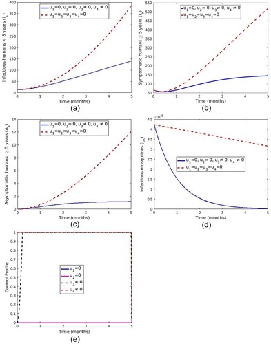
5.1.1. Strategy A: control with LLINs and spray of insecticide

This strategy combines protection using LLINs ($u_1(t)$) and vector control effort using spraying of insecticide ($u_4(t)$). The sizes of infectious individuals and mosquitoes in Figure 8( a–d) are reduced with control compared to the situation without controls. Figure 8(e) shows that the optimal use of LLINs $u_1(t)$ and $u_4(t)$ are at the upper bound for the entire time of intervention.

Figure 8. Impact of use of LLINs and spray of insecticide on malaria transmission dynamics.

5.1.2. Strategy B: control with the treatment of symptomatic infections and spray of insecticide

This strategy uses treatment of symptomatic individuals ($u_2(t)$) and spraying of insecticide ($u_4(t)$). Figure 9( a–d) shows a significant difference in the number of infectious under five years children, symptomatic adult individuals, asymptomatic carriers and infectious mosquitoes with control compared to those without controls. Optimal control profile Figure 9(e) reveals that control $u_2(t)$ and $u_4(t)$ is maintained at the upper limit throughout the entire time of intervention.

Figure 9. Simulation showing optimal use of treatment of symptomatic human and spray of insecticide.

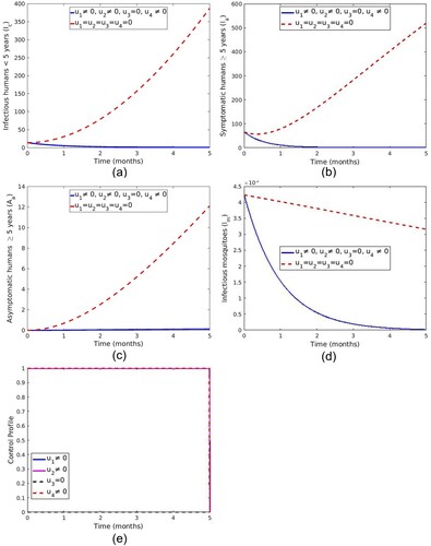
5.1.3. Strategy C: control with screening and treatment of asymptomatic carrier and spray of insecticide

In this strategy, screening and treatment of asymptomatic carriers ($u_3(t)$) and vector control effort using spraying of insecticide ($u_4(t)$) are used together to optimize the objective function in (20(20) $J(u_1,u_2,u_3,u_4)={\int }_0^{t_f}(A_1{I}_c+A_2{I}_a+A_3{A}_a+B_1{S}_m+B_2{E}_m+B_3{I}_m+P)\mathrm{d}t$(20) ). In contrast, LLINs ($u_1(t)$) and treatment of symptomatic ($u_2(t)$) are set to zero. It can be observed that the number of infectious individuals and mosquitoes in Figure 10( a–d) is significantly different with control compared to the case without controls. Figure 10(e) shows that the optimal use of screening and treatment of asymptomatic carriers $u_3(t)$ starts at a lower rate and increases to a maximum at 0.23 months while a spray of insecticide $u_4(t)$ is at upper bound for the entire time of intervention.

Figure 10. Simulations depicting optimal use of screening and treatment of asymptomatic carrier ($u_3(t)$) and spray of insecticide ($u_4(t)$).

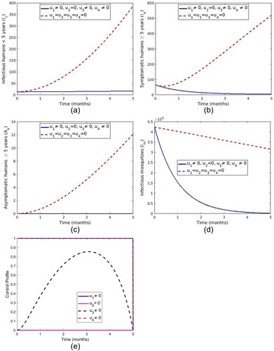
5.1.4. Strategy D: control with LLINs, treatment of symptomatic human and spray of insecticide

Optimizing the objective function (20(20) $J(u_1,u_2,u_3,u_4)={\int }_0^{t_f}(A_1{I}_c+A_2{I}_a+A_3{A}_a+B_1{S}_m+B_2{E}_m+B_3{I}_m+P)\mathrm{d}t$(20) ) using LLINs ($u_1(t)$), treatment of symptomatic infections ($u_2(t)$) and spraying of insecticide ($u_4(t)$) while the screening and treatment of asymptomatic carrier ($u_3(t)$) is set to zero. The results in Figure 11( a–d) show a reduced number of infectious human ($I_c$, $I_a$ and $A_a$) and infectious mosquitoes with control compared to the situation without controls. Figure 11(e) shows that the optimal use of LLINs ($u_1(t)$), treatment of symptomatic individuals $u_2(t)$ and spray of insecticide is at the upper bound for the entire time of intervention.

Figure 11. Simulation of the malaria model showing the effect of the optimal controls $u_1(t)$, $u_2(t)$ and $u_4(t)$.

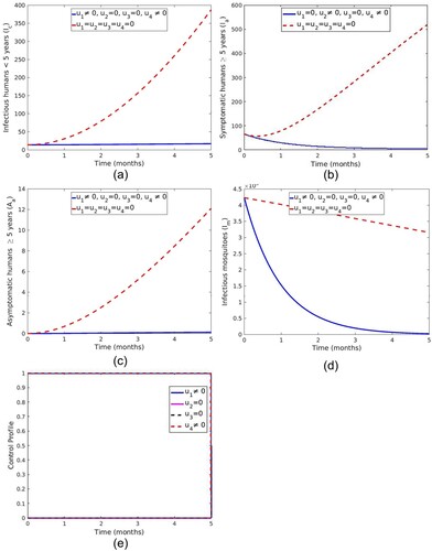
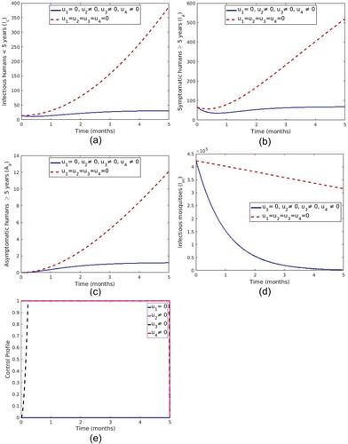
5.1.5. Strategy E: control with LLINs, screening and treatment of asymptomatic carriers and a spray of insecticide

The control measures $u_1(t)$, $u_3(t)$ and $u_4(t)$ are applied while control measure $u_2(t)$ is set to zero. Figure 12( a–d) show a reduced number of infectious humans ($I_c$, $I_a$ and $A_a$) and infectious mosquitoes with control compared to those without controls. It can be noted from Figure 12(e) that the optimal use of LLINs ($u_1(t)$) and spray of insecticide is maintained at upper bound for the entire time of intervention. In contrast, the optimal control $u_3(t)$ increases to 0.86 at t = 3 months before it drops gradually to the lower limit at the final time.

Figure 12. Impact of use of LLINs, screening and treatment of asymptomatic carrier and spray of insecticide.

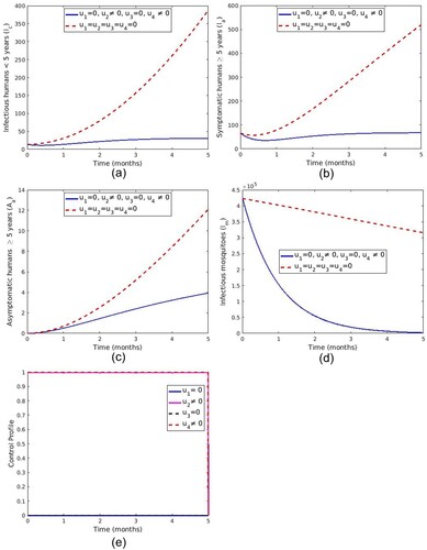
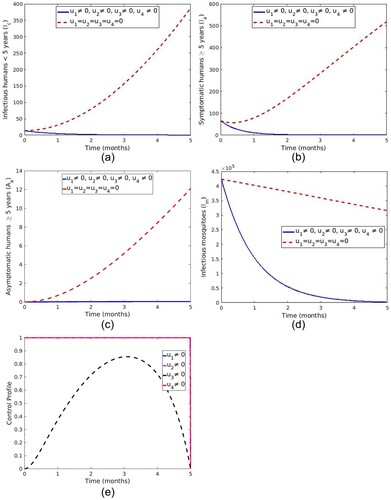
5.1.6. Strategy F: control with the treatment of symptomatic individuals, screening and treatment of asymptomatic carriers and spray of insecticide

In this strategy the control $u_2(t)$, $u_3(t)$ and $u_4(t)$ are applied and only LLINs $u_1(t)$ is set to zero. Figure 13( a–d) shows a significant difference in the number of infectious humans ($I_c$, $I_a$ and $A_a$) and infectious mosquitoes with control compared to those without controls. It can be observed from Figure 13(e) that the optimal use of treatment of symptomatic humans ($u_2(t)$) and spray of insecticide $u_4(t)$ is maintained at the upper limit throughout the time of intervention while screening and treatment of asymptomatic carrier $u_3(t)$ starts at a lower rate and increases to a maximum at t = 0.23 months.

Figure 13. Impact of use of $u_1(t)$, $u_2(t)$, $u_3(t)$ and $u_4(t)$.

5.1.7. Strategy G: control with LLINs, treatment of symptomatic humans, screening and treatment of asymptomatic carriers and a spray of insecticide

In this strategy all four controls $u_1(t)$,$u_2(t)$, $u_3(t)$ and $u_4(t)$ are applied to optimize the objective function (20(20) $J(u_1,u_2,u_3,u_4)={\int }_0^{t_f}(A_1{I}_c+A_2{I}_a+A_3{A}_a+B_1{S}_m+B_2{E}_m+B_3{I}_m+P)\mathrm{d}t$(20) ). As shown in Figure 14( a–d), the control resulted in a decrease in the number of infected humans ($I_c$, $I_a$ and $A_a$) and infectious mosquitoes ($I_m$) with control compared to the number in the case without control. Figure 14(e) reveal that the optimal use of LLINs ($u_1(t)$), treatment of symptomatic individuals, screening and treatment of asymptomatic carrier and spray of insecticide is maintained at upper bound for the entire time of intervention while the optimal control $u_3(t)$ increases to 0.8553 at t = 3 months before it drops gradually to the minimum at the final time.

Figure 14. Impact of use of $u_2(t)$, $u_3(t)$ and $u_4(t)$.

The simulation result revealed that, with control strategies, the number of months required to eliminate malaria in the community is significantly reduced compared to when no control strategy is implemented. This means that the control strategies have a positive impact, reducing the number of infected humans and mosquitoes. Apart from that, from all strategies used in this study, we found that the control strategy incorporating all four control interventions gives better results as it reduces the number of infected humans in a few months compared to other control strategies. However, in the presence of limited resources, it is essential to consider cost-effectiveness analysis to determine the cost and benefits of each strategy to obtain the best control strategy for implementation. Therefore, each strategy's cost-effectiveness analysis is performed in the next section.

5.2. Cost-effective analysis

Cost-effective analysis (CEA) is a form of economic evaluation that compares the relative costs and outcomes of different control strategies. The cost-effectiveness analysis helps us obtain the most cost-effective strategy to apply in case of scarce resources. To determine the most beneficial and cost-effective control strategy to use, the cost-effective incremental ratio (ICER) is employed. The ICER is described as the additional cost per additional health outcome. The difference between the cost and the health benefits of the two competing intervention strategies is compared. Each intervention is compared to the next less effective alternatives. That is (26) $\mathrm{ICER}=\frac{\mathrm{Differences}\mathrm{in}\mathrm{cost}\mathrm{of}\mathrm{interventions}\mathrm{strategies}}{\mathrm{Differences}\mathrm{in}\mathrm{number}\mathrm{of}\mathrm{infection}\mathrm{averted}\mathrm{by}\mathrm{the}\mathrm{strategies}}=\frac{\mathrm{\Delta }{C}_T}{\mathrm{\Delta }{E}_T},$(26) where $C_T$ is the total cost for implementing a particular strategy and $E_T$ is a total infection averted. The total cost associated with each strategy is given by (27) $C_T={\int }_0^{t_f}(C_1{u}_1(t)N_h+C_2{u}_2(t)(I_c+I_a)+C_3{u}_3(t)A_a+C_4{u}_4(t)(S_m+E_m+I_m))dt$(27) where $N_h=S_c+E_c+I_c+R_c+S_a+E_a+I_a+A_a+R_a$, $C_1$ is per person unit cost for LLINs use, $C_2$ presents per person unit cost of treatment of symptomatic individuals, $C_3$ corresponds to per person cost of screening and treatment of asymptomatic carrier and $C_4$ is per mosquito cost following a spray of insecticide. The total number of infections averted is obtained by subtracting the total number of infections with control from the total number of infections without control. For example, the total infections averted by strategy A is given by the difference between the total number of infections when no control was used and the number of infections when strategy A was used, i.e. 222,390,036−49,654,344=172,735,692.

The optimality system based on the control strategies in subsection 5.1 is simulated to implement the ICER. The total number of infections averted and the total cost are presented in Table 5. The parameters used are as in Table 4.

Table 5. Number of infections averted and total cost of each strategy.

Strategy	Infections	Total infections averted ($E_T$)	Total costs ($C_T$)
No strategy	222,390,036	–	–
A	49,654,344	172,735,692	29,578,264.19
B	49,683,050	172,706,986	6,067,738.64
C	49,739,187	172,650,849	6,066,953.99
D	49,641,369	172,748,667	29,578,410.03
E	49,654,323	172,735,713	29,578,264.43
F	49,682,381	172,707,655	6,067,750.46
G	49,641,348	172,748,688	29,578,410.28

The control strategies from Table 5 are ranked in order of increasing effectiveness based on infections averted. The incremental effectiveness $\mathrm{\Delta }{E}_T$ and the incremental cost $\mathrm{\Delta }{C}_T$ are determined using (26(26) $\mathrm{ICER}=\frac{\mathrm{Differences}\mathrm{in}\mathrm{cost}\mathrm{of}\mathrm{interventions}\mathrm{strategies}}{\mathrm{Differences}\mathrm{in}\mathrm{number}\mathrm{of}\mathrm{infection}\mathrm{averted}\mathrm{by}\mathrm{the}\mathrm{strategies}}=\frac{\mathrm{\Delta }{C}_T}{\mathrm{\Delta }{E}_T},$(26) ). The ICER is then obtained by dividing $\mathrm{\Delta }{E}_T$ by $\mathrm{\Delta }{C}_T$ as in (26(26) $\mathrm{ICER}=\frac{\mathrm{Differences}\mathrm{in}\mathrm{cost}\mathrm{of}\mathrm{interventions}\mathrm{strategies}}{\mathrm{Differences}\mathrm{in}\mathrm{number}\mathrm{of}\mathrm{infection}\mathrm{averted}\mathrm{by}\mathrm{the}\mathrm{strategies}}=\frac{\mathrm{\Delta }{C}_T}{\mathrm{\Delta }{E}_T},$(26) ). To compare intervention strategies incrementally, the ICER for two competing strategies, for example, C and B, is calculated as follows: $\begin{array}{rl}\mathrm{ICER}(\mathrm{C})& =\frac{6,066,953.99-0}{172,650,849-0}=0.035,\\ \mathrm{ICER}(\mathrm{B})& =\frac{6,067,738.64-6,066,953.99}{172,706,986-172,650,849}=\mathrm{0.0139.}\end{array}$The results are given in Table 6.

Comparison between strategy C and B shows that ICER(B)< ICER (C), indicating that strategy C is more costly and less effective than strategy B. Thus, strategy C is excluded from the alternatives and recalculated ICER for the remaining strategies, and the results are as shown in Table 7.

Table 7. Incremental cost-effectiveness ratios for optimal control strategies B, F, A, E, D and G.

Strategies	E	$\mathrm{\Delta }{E}_T$	C	$\mathrm{\Delta }{C}_T$	ICER
B	172,706,986	172,706,986	, 6067,738.64	6,067,738.64	0.0351
F	172,707,655	669	6,067,750.46	11.82	0.0177
A	172,735,692	28,037	29,578,264.19	23,510,513.73	838.5531
E	172,735,713	21	29,578,264.43	0.24	0.0114
D	172,748,667	12954	29,578,410.03	145.60	0.0112
G	172,748,688	21	29,578,410.28	0.25	0.0119

That is the ICER for strategy B, and F is given by $\begin{array}{rl}\mathrm{ICER}(\mathrm{B})& =\frac{6,067,738.64}{172,706,986}=0.03513314,\\ \mathrm{ICER}(\mathrm{F})& =\frac{6,067,750.46-6,067,738.64}{172,707,655--172,706,986}=\mathrm{0.0177.}\end{array}$Similarly, it is observed that the ICER for strategy F is less than for strategy B. Hence, strategy B is more expensive than strategy F. Therefore, strategy B is excluded and recomputes ICER for the remaining strategies as shown in Table 8.

Table 8. Incremental cost-effectiveness ratios for optimal control strategies F, A, E, D and G.

Strategies	E	$\mathrm{\Delta }{E}_T$	C	$\mathrm{\Delta }{C}_T$	ICER
F	172,707,655	172,707,655	6,067,750.46	6,067,750.46	0.0351
A	172,735,692	28,037	29,578,264.19	23,510,513.73	838.5531
E	172,735,713	21	29,578,264.43	0.24	0.0114
D	172,748,667	12,954	29,578,410.03	145.60	0.0112
G	172,748,688	21	29,578,410.28	0.25	0.0119

From Table 8, $\begin{array}{rl}\mathrm{ICER}(\mathrm{F})& =\frac{6,067,750.46}{172,707,655}=0.03513307,\\ \mathrm{ICER}(\mathrm{A})& =\frac{29,578,264.19-6,067,750.46}{172,735,692-172,707,655}=\mathrm{838.5531.}\end{array}$It is observed that strategy A's ICER is higher than strategy F. Thus, strategy A is more expensive and less effective than strategy F. Therefore, strategy A is omitted from the alternatives. We recalculate the ICER and compare strategies F and E in Table 9.

Table 9. Incremental cost-effectiveness ratios for optimal control strategies F, E, D and G.

Strategies	E	$\mathrm{\Delta }{E}_T$	C	$\mathrm{\Delta }{C}_T$	ICER
F	172,707,655	172,707,655	6,067,750.46	6,067,750.46	0.0351
E	172,735,713	28,058	29,578,264.43	23,510,513.97	837.9255
D	172,748,667	12,954	29,578,410.03	145.60	0.0112
G	172,748,688	21	29,578,410.28	0.25	0.0119

It is observed that ICER(E)> ICER(F), which implies that control strategy E is more costly and less effective than strategy F. Hence, strategy E is excluded from the list of strategies. We recalculate the ICER and compare strategies F and D as shown in Table 10.

Table 10. Incremental cost-effectiveness ratios for optimal control strategies F, D and G.

Strategies	E	$\mathrm{\Delta }{E}_T$	C	$\mathrm{\Delta }{C}_T$	ICER
F	172,707,655	172,707,655	6,067,750.46	6,067,750.46	0.0351
D	172,748,667	41,012	29,578,410.03	23,510,659.57	573.2629
G	172,748,688	21	29,578,410.28	0.25	0.0119

The comparison between strategy F and D indicates that strategy D is more expensive than strategy F as ICER for strategy F is less than the ICER for strategy D, as shown in Table 10. Therefore, strategy D is excluded from the set of alternatives and strategies F and G are compared. We recalculate ICER for the remaining strategies as shown in Table 11.

Table 11. Incremental cost-effectiveness ratios for optimal control strategies F and G.

Strategies	E	$\mathrm{\Delta }{E}_T$	C	$\mathrm{\Delta }{C}_T$	ICER
F	172,707,655	172,707,655	6,067,750.46	6,067,750.46	0.0351
G	172,748,688	41,033	29,578,410.28	23,510,659.82	572.9696

Lastly, the comparison between strategy F and strategy G (Table 11) indicates that strategy F is less costly and more effective than strategy G (ICER (F) < ICER (G)). We conclude that strategy F (treatment of symptomatic, screening and treatment of asymptomatic carrier and spray of insecticide) is the most cost-effective of all strategies in case of limited resources. Hence it is the best control strategy.

6. Conclusion

An age-structured deterministic model for malaria transmission that includes symptomatic carriers and temperature variability is derived. The model is analysed when temperature-dependent parameters are kept constant. The basic reproduction number of the model is determined, and the stability of disease-free equilibrium is proved. A sensitivity analysis of the parameters of the basic reproduction number has been done. The results show that mosquitoes biting and death rates are the most sensitive parameters. Also, it has been observed that parameters related to children under five are more important than the corresponding parameters in individuals aged five years and above. Similarly, the recovery rate of asymptomatic carriers is relatively more important than the recovery rate of symptomatic individuals. Thus, interventions to reduce the biting rate and increase the death rate of mosquitoes have a greater impact on reducing disease transmission. Besides that, controlling the disease in children and symptomatic carries will have a high impact.

Furthermore, the model was extended to incorporate temperature-dependent parameters. Temperature variability is captured using the cosine function. The function is fitted to the monthly mean maximum temperature data for the Iringa region from 2016 to 2020 to calibrate the temperature-dependent parameters. The model (1(1) $\begin{array}{r}\begin{array}{ll}{\displaystyle \frac{\mathrm{d}{S}_c}{\mathrm{d}t}}& ={\mathrm{\Lambda }}_c+{\eta }_c{R}_c-({\mu }_h+{\lambda }_c(T)+\zeta )S_c,\\ {\displaystyle \frac{\mathrm{d}{E}_c}{\mathrm{d}t}}& ={\lambda }_c(T)S_c-({\mu }_h+{\sigma }_c+\zeta )E_c,\\ {\displaystyle \frac{\mathrm{d}{I}_c}{\mathrm{d}t}}& ={\sigma }_c{E}_c-({\mu }_h+{\delta }_c+\zeta +{\gamma }_c)I_c,\\ {\displaystyle \frac{\mathrm{d}{R}_c}{\mathrm{d}t}}& ={\gamma }_c{I}_c-(\zeta +{\mu }_h+{\eta }_c)R_c,\\ {\displaystyle \frac{\mathrm{d}{S}_a}{\mathrm{d}t}}& =\zeta S_c+{\eta }_a{R}_a-({\mu }_h+{\lambda }_a(T))S_a,\\ {\displaystyle \frac{\mathrm{d}{E}_a}{\mathrm{d}t}}& ={\lambda }_a(T)S_a+\zeta E_c-[{\mu }_h+{\sigma }_a\theta +(1-\theta ){\sigma }_a]E_a,\\ {\displaystyle \frac{\mathrm{d}{I}_a}{\mathrm{d}t}}& ={\sigma }_a\theta E_a+\zeta I_c-[{\mu }_h+{\delta }_a+{\gamma }_s]I_a,\\ {\displaystyle \frac{\mathrm{d}{A}_a}{\mathrm{d}t}}& ={\sigma }_a(1-\theta )E_a-({\mu }_h+{\gamma }_a)A_a,\\ {\displaystyle \frac{\mathrm{d}{R}_a}{\mathrm{d}t}}& ={\gamma }_a{A}_a+{\gamma }_s{I}_a+\zeta R_c-({\mu }_h+{\eta }_a)R_a,\\ {\displaystyle \frac{\mathrm{d}{S}_m}{\mathrm{d}t}}& ={\mathrm{\Lambda }}_m(T)-({\mu }_m(T)+{\lambda }_m(T))S_m,\\ {\displaystyle \frac{\mathrm{d}{E}_m}{\mathrm{d}t}}& ={\lambda }_m(T)S_m-({\mu }_m(T)+{\sigma }_m(T))E_m,\\ {\displaystyle \frac{\mathrm{d}{I}_m}{\mathrm{d}t}}& ={\sigma }_m(T)E_m-{\mu }_m(T)I_m,\end{array}\}\end{array}$(1) ) was parameterized using malaria case data for the Iringa region in Tanzania from 2016 to 2018. Moreover, the model system is validated using real data for malaria cases in Iringa from 2019 to 2020. The system fits well with these data. Effects of temperature variability have been performed, and the results show that optimal cumulative malaria new cases are obtained when the temperature in the absence of seasonality is in the range 24.78${}^{\mathrm{o}}$C to 26.78${}^{\mathrm{o}}$C. So the temperature below or above this range has reduced cumulative malaria new cases.

To control the transmission of malaria in a community, the model (1(1) $\begin{array}{r}\begin{array}{ll}{\displaystyle \frac{\mathrm{d}{S}_c}{\mathrm{d}t}}& ={\mathrm{\Lambda }}_c+{\eta }_c{R}_c-({\mu }_h+{\lambda }_c(T)+\zeta )S_c,\\ {\displaystyle \frac{\mathrm{d}{E}_c}{\mathrm{d}t}}& ={\lambda }_c(T)S_c-({\mu }_h+{\sigma }_c+\zeta )E_c,\\ {\displaystyle \frac{\mathrm{d}{I}_c}{\mathrm{d}t}}& ={\sigma }_c{E}_c-({\mu }_h+{\delta }_c+\zeta +{\gamma }_c)I_c,\\ {\displaystyle \frac{\mathrm{d}{R}_c}{\mathrm{d}t}}& ={\gamma }_c{I}_c-(\zeta +{\mu }_h+{\eta }_c)R_c,\\ {\displaystyle \frac{\mathrm{d}{S}_a}{\mathrm{d}t}}& =\zeta S_c+{\eta }_a{R}_a-({\mu }_h+{\lambda }_a(T))S_a,\\ {\displaystyle \frac{\mathrm{d}{E}_a}{\mathrm{d}t}}& ={\lambda }_a(T)S_a+\zeta E_c-[{\mu }_h+{\sigma }_a\theta +(1-\theta ){\sigma }_a]E_a,\\ {\displaystyle \frac{\mathrm{d}{I}_a}{\mathrm{d}t}}& ={\sigma }_a\theta E_a+\zeta I_c-[{\mu }_h+{\delta }_a+{\gamma }_s]I_a,\\ {\displaystyle \frac{\mathrm{d}{A}_a}{\mathrm{d}t}}& ={\sigma }_a(1-\theta )E_a-({\mu }_h+{\gamma }_a)A_a,\\ {\displaystyle \frac{\mathrm{d}{R}_a}{\mathrm{d}t}}& ={\gamma }_a{A}_a+{\gamma }_s{I}_a+\zeta R_c-({\mu }_h+{\eta }_a)R_a,\\ {\displaystyle \frac{\mathrm{d}{S}_m}{\mathrm{d}t}}& ={\mathrm{\Lambda }}_m(T)-({\mu }_m(T)+{\lambda }_m(T))S_m,\\ {\displaystyle \frac{\mathrm{d}{E}_m}{\mathrm{d}t}}& ={\lambda }_m(T)S_m-({\mu }_m(T)+{\sigma }_m(T))E_m,\\ {\displaystyle \frac{\mathrm{d}{I}_m}{\mathrm{d}t}}& ={\sigma }_m(T)E_m-{\mu }_m(T)I_m,\end{array}\}\end{array}$(1) ) is extended to an optimal control problem using four time-dependent controls: personal protection using LLINs, treatment of symptomatic, screening and treatment of asymptomatic carriers and vector control (spray of insecticide). Theoretical analysis of the optimal control system (19(19) $\begin{array}{r}\begin{array}{ll}{\displaystyle {\displaystyle \frac{\mathrm{d}{S}_c}{\mathrm{d}t}}}& ={\mathrm{\Lambda }}_c+{\eta }_c{R}_c-(1-w_c{u}_1){\lambda }_c(T)S_c-({\mu }_h+\zeta )S_c,\\ {\displaystyle {\displaystyle \frac{\mathrm{d}{E}_c}{\mathrm{d}t}}}& =(1-w_c{u}_1){\lambda }_c(T)S_c-({\mu }_h+{\sigma }_c+\zeta )E_c,\\ {\displaystyle {\displaystyle \frac{\mathrm{d}{I}_c}{\mathrm{d}t}}}& ={\sigma }_c{E}_c-({\mu }_h+{\delta }_c+\zeta +{\gamma }_c+u_2\tau )I_c,\\ {\displaystyle {\displaystyle \frac{\mathrm{d}{R}_c}{\mathrm{d}t}}}& =({\gamma }_c+u_2\tau )I_c-(\zeta +{\mu }_h+{\eta }_c)R_c,\\ {\displaystyle {\displaystyle \frac{\mathrm{d}{S}_a}{\mathrm{d}t}}}& =\zeta S_c+{\eta }_a{R}_a-({\mu }_h+(1-w_a{u}_1){\lambda }_a(T))S_a,\\ {\displaystyle {\displaystyle \frac{\mathrm{d}{E}_a}{\mathrm{d}t}}}& =(1-w_a{u}_1){\lambda }_a(T)S_a+\zeta E_c-[{\mu }_h+{\sigma }_a\theta +(1-\theta ){\sigma }_a]E_a,\\ {\displaystyle {\displaystyle \frac{\mathrm{d}{I}_a}{\mathrm{d}t}}}& ={\sigma }_a\theta E_a+\zeta I_c-[{\mu }_h+{\delta }_a+({\gamma }_s+u_2\tau )]I_a,\\ {\displaystyle {\displaystyle \frac{\mathrm{d}{A}_a}{\mathrm{d}t}}}& ={\sigma }_a(1-\theta )E_a-({\mu }_h+{\gamma }_a+u_3\tau )A_a,\\ {\displaystyle {\displaystyle \frac{\mathrm{d}{R}_a}{\mathrm{d}t}}}& =({\gamma }_a+u_3\tau )A_a+({\gamma }_s+u_2\tau )I_a+\zeta R_c-({\mu }_h+{\eta }_a)R_a,\\ {\displaystyle {\displaystyle \frac{\mathrm{d}{S}_m}{\mathrm{d}t}}}& ={\mathrm{\Lambda }}_m(T)-{\lambda }_m(T)S_m-({\mu }_m(T)+w_m{u}_4)S_m,\\ {\displaystyle {\displaystyle \frac{\mathrm{d}{E}_m}{\mathrm{d}t}}}& ={\lambda }_m(T)S_m-({\sigma }_m+{\mu }_m(T)+w_m{u}_4)E_m,\\ {\displaystyle {\displaystyle \frac{\mathrm{d}{I}_m}{\mathrm{d}t}}}& ={\sigma }_m{E}_m-({\mu }_m(T)+w_m{u}_4)I_m,\end{array}\}\end{array}$(19) ) is carried out. The system is simulated to investigate the impact of combining at least two controls – with vector control measures included – on malaria transmissions. The simulation was performed using the temperature value with the highest malaria cases (i.e. $T={26.3}^{\mathrm{o}}$C ). It is shown that the sizes of infected humans and mosquitoes are minimized with all combinations of control variables. The findings further indicate that the control strategy comprising all four control measures (i.e. LLINs, treatment of symptomatic, screening and treatment of asymptomatic carriers and spray of insecticides) significantly reduces malaria transmission among humans and mosquitoes than any other combination used.

However, the cost-effectiveness analysis indicates that the combination of optimal use of symptomatic treatment, screening and treatment of asymptomatic and insecticide spray is the most cost-effective intervention strategy of all combinations considered in this work. Therefore, it is suggested that in case of limited resources, treatment of symptomatic individuals, screening and treatment of asymptomatic carriers and spray of insecticides should be used since it is cheap and effective in reducing disease transmission.

Disclosure statement

No potential conflict of interest was reported by the author(s).

Additional information

Funding

‘This work was funded by a grant from the African Institute for Mathematical Sciences, www.nexteinstein.org, with financial support from the Government of Canada, provided through Global Affairs Canada, www.international.gc.ca, and the International Development Research Centre, www.idrc.ca’. Also, the corresponding author acknowledges with gratitude the Ministry of Education, Science and Technology – Tanzania for financial support.

References

- G.J. Abiodun, P.J. Witbooi, K.O. Okosun, and R. Maharaj, Exploring the impact of climate variability on malaria transmission using a dynamic mosquito-human malaria model, Open Infect. Dis. J. 10(1) (2018), pp. 88–100.
- J.M. Addawe and J.E.C. Lope, Sensitivity analysis of the age-structured malaria transmission model, AIP Conf. Proc. 1482(1) (2012), pp. 47–53. doi:10.1063/1.4757436
- J.M. Addawe and A.K. Pajimola, Dynamics of climate-based malaria transmission model with the age-structured human population, AIP. Conf. Proc. 1782(1) (2016), pp. 040002. doi:10.1063/1.4966069
- F.B. Agusto, Optimal control and temperature variations of malaria transmission dynamics, Complexity 2020 (2020), pp. 1–32.
- F.B. Agusto, A.B. Gumel, and P.E. Parham, Qualitative assessment of the role of temperature variations on malaria transmission dynamics, J. Biol. Syst. 23(04) (2015), pp. 1550030.
- S. Altizer, A. Dobson, P. Hosseini, P. Hudson, M. Pascual, and P. Rohani, Seasonality and the dynamics of infectious diseases, Ecol. Lett. 9(4) (2006), pp. 467–484.
- N. Chitnis , J.M. Hyman, and J.M. Cushing, Determining important parameters in the spread of malaria through the sensitivity analysis of a mathematical model, Bull. Math. Biol. 70(5) (2008), pp. 1272–1296.
- B. Dembele, A. Friedman, and A.A. Yakubu, Malaria model with periodic mosquito birth and death rates, J. Biol. Dyn. 3(4) (2009), pp. 430–445.
- A. Egbendewe-Mondzozo, M. Musumba, B.A. McCarl, and X. Wu, Climate change and vector-borne diseases: An economic impact analysis of malaria in Africa, Int. J. Environ. Res. Pub. He. 8(3) (2011), pp. 913–930.
- F. Forouzannia and A.B. Gumel, Mathematical analysis of an age-structured model for malaria transmission dynamics, Math. Biosci. 247 (2014), pp. 80–94.
- S.M. Garba and U.A. Danbaba, Modeling the effect of temperature variability on malaria control strategies, Math. Model. Nat. Phenom. 15 (2020), pp. 65.
- A.K. Githeko, S.W. Lindsay, U.E. Confalonieri, and J.A. Patz, Climate change and vector-borne diseases: A regional analysis, Bull. World He. Organ. 78 (2000), pp. 1136–1147.
- A. Hugo, O.D. Makinde, S. Kumar, and F.F. Chibwana, Optimal control and cost effectiveness analysis for newcastle disease eco-epidemiological model in Tanzania, J. Biol. Dyn. 11(1) (2017), pp. 190–209.
- A.S. Kalula, E. Mureithi, T. Marijani, and I. Mbalawata, An age-structured model for transmission dynamics of malaria with infected immigrants and asymptomatic carriers, Tanz. J. Sci. 47(3) (2021), pp. 953–968.
- J.C. Kamgang and G. Sallet, Computation of threshold conditions for epidemiological models and global stability of the disease-free equilibrium (DFE), Math. Biosci. 213(1) (2008), pp. 1–12.
- B.J. Mafwele and J.W. Lee, Relationships between transmission of malaria in Africa and climate factors, Sci. Rep. 12(1) (2022), pp. 1–8.
- O.D. Makinde and K.O. Okosun, Impact of chemo-therapy on optimal control of malaria with disease infected immigrants, Biol. Syst. 104 (2011), pp. 32–41.
- M. Martcheva, An Introduction to Mathematical Epidemiology, Springer, NewYork, 2013.
- E.A. Mordecai, Optimal temperature for malaria transmission is dramatically lower than previously predicted, Ecol. Lett. 16(1) (2013), pp. 22–30.
- G.G. Mwanga , H. Haario, and V. Capasso, Optimal control problems of epidemic systems with parameter uncertainties: Application to a malaria two-age-classes transmission model with asymptomatic carriers, Math. Biosci. 261 (2015), pp. 1–12.
- E.T. Ngarakana-Gwasira, C.P. Bhunu, M. Masocha, and E. Mashonjowa, Assessing the role of climate change in malaria transmission in Africa, Malar. Res. Treat. 2016 (2016), pp. 7104291. doi:10.1155/2016/7104291
- K.O. Okosun, O. Rachid, and N. Marcus, Optimal control strategies and cost-effectiveness analysis of a malaria model, BioSystems 111(2) (2013), pp. 83–101.
- K. Okuneye and A.B. Gumel, Analysis of a temperature- and rainfall-dependent model for malaria transmission dynamics, Math. Biosci. 287 (2017), pp. 72–92.
- S. Olaniyi, K.O. Okosun, S.O. Adesanya, and R.S. Lebelo, Modelling malaria dynamics with partial immunity and protected travellers: Optimal control and cost-effectiveness analysis, J. Biol. Dyn. 14(1) (2020), pp. 90–115.
- P.E. Parham and E. Michael, Modelling climate change and malaria transmission, in Model. Parasite Trans. Control 2010. pp. 184–199
- P.E. Parham, J. Waldock, G.K. Christophides, D. Hemming, F. Agusto, K.J. Evans, N. Fefferman, H. Gaff, A. Gumel, S. LaDeau, and S. Lenhart, Climate, environmental and socio-economic change: Weighing up the balance in vector-borne disease transmission, Philos. Trans. R Soc. B Biol. Sci.370(1665) (2015), pp. 20130551.
- R.F. Schumacher and E. Spinelli, Malaria in children, Mediterr. J. Hematol. Infect. Dis. 92 (2012), pp. 2035–3006.
- S.Y. Tchoumi, E.Z. Dongmo, J.C. Kamgang, and J.M. Tchuenche, Dynamics of a two-group structured malaria transmission model, Inform. Med. Unlocked 29 (2022), pp. 100897.
- P. van den Driessche and J. Watmough, Reproduction number and subthreshold endemic equilibria for compartment models of disease transmission, Math. Biosci. 180(1-2) (2002), pp. 29–48.
- World Health Organization, World Malaria Report, 2020. Available at https://www.who.int/publications/i/item/9789240015791. Accessed on March 8, 2021.