The interplay between multiple control mechanisms in a host–parasitoid system: a discrete-time stage-structured modelling approach

Abstract

We propose a discrete-time host–parasitoid model with stage structure in both species. For this model, we establish conditions for the existence and global stability of the extinction and parasitoid-free equilibria as well as conditions for the existence and local stability of an interior equilibrium and system persistence. We study the model numerically to examine how pesticide spraying may interact with natural enemies (parasitoids) to control the pest (host) species. We then extend the model to an impulsive difference system that incorporates both periodic pesticide spraying and augmentation of the natural enemies to suppress the pest population. For this system, we determine when the pest-eradication periodic solution is globally attracting. We also examine how varying the control measures (pesticide concentration, natural enemy augmentation and the frequency of applications) may lead to different pest outbreak or persistence outcomes when eradication does not occur.

Keywords:

• Host–parasitoid
• stage structure
• impulsive difference equations
• integrated pest management
• global dynamics

     Dedicated to the memory of Abdul-Aziz Yakubu.

1. Introduction

Biological control refers to the use of a natural enemy, such as a predator, parasitoid or pathogen, to suppress a pest population. These natural enemies are released either periodically in small numbers, referred to as inoculative release, or all at once in large quantities, referred to as inundative release [17]. For example, the periodic introduction of the parasitoid Encarsia formosa has been found to be effective at controlling the greenhouse whitefly, Trialeurodes vaporariorum, a serious pest of tomato and cucumber crops [2]. Insect parasitoids are the most commonly utilized biological control agents [13]. The larvae of parasitoids grow inside or on a host which they eventually kill [25].

Integrative pest management (IPM) schemes employ a number of strategies, such as biological and chemical controls (e.g. pesticides or insecticides), to suppress a pest species [20]. Since single chemical control strategies frequently fail as a result of evolution of resistance in the pest, these schemes often use chemical control in conjunction with biological control agents to reduce the abundance of a pest. However, the compatibility of these controls is critical to the success of an integrated pest management strategy [12, 24, 36, 37]. Not only may different natural enemies vary widely in the response to toxicants, but variation in population structure may also impact results. For example, Diaeretiella rapae (M'Intosh), a common parasitoid of the cabbage aphid, was shown to experience differential stage susceptibility to the insecticide imidacloprid, with mortality in the adult stage being more than double that of the pupae (mummy) stage for various concentrations of the insecticide [37].

There are many existing mathematical models of host–parasitoid systems (see  [27] and the references therein). One of the earliest discrete-time host–parasitoid models was developed by Thompson in 1924, while the more familiar Nicholson–Bailey model was developed later in 1935. A modification to the Nicholson–Bailey model with type-II functional responses was developed by Holling in 1959. This model is the first to assume that the parasitoid is search limited, in contrast to Thompson's model which assumed the parasitoid is egg-limited. The differential equation system developed independently by Lotka (1925) and Volterra (1926) for predator–prey interactions has also been used as a basis for modelling host–parasitoid interactions in continuous time  [27]. Ample extensions of these foundational host–parasitoid models have been developed to describe different host–parasitoid scenarios. These includes host–parasitoid models with different nonlinearities [4, 16, 17, 30, 31], with different functional responses  [32, 33], with Allee effects in the host  [15, 21, 22], with stage structure  [3, 6, 15, 35, 42], age structure [5], and co-evolution between host and parasitoid  [11, 29]. Numerous integrated pest management host–parasitoid systems have also been developed, including  [10, 20, 38–41, 43, 44]. These impulsive difference systems assume that control measures consisting of both chemical control and the release of natural enemies such as parasitoids are applied either periodically or when the pest (host) density reaches a designated economic threshold. However, we note that these systems often assume unstructured populations.

Motivated by the distinctive developmental stages often observed in both hosts and parasitoids as well as the observation that both species may exhibit stage-specific differential susceptibility to toxicants [37], in this paper we develop a discrete-time host–parasitoid model with stage structure in both species. Specifically, we assume individuals in each species are classified according to two developmental stages, either juvenile or adult, resulting in a four-dimensional system. We first provide a rigorous analysis of the equilibria dynamics and persistence of this system. Then, viewing the host as a pest species, we use the system to consider integrated pest management interventions that consist of both biological control (i.e. the parasitoid) and chemical control via the release of a pesticide.

We first consider the case where control measures are continuous leading to pesticide-induced mortality in every time unit. We find that the effectiveness of the combined management strategies depends heavily on the timing of pesticide spray (e.g. at the beginning versus end of the time unit), the susceptibility of the parasitoid to the pesticide and the type of attractor to which the system converges. In particular, when time series solutions are attracted to equilibria, then both spraying at the end of the time unit and pesticide-induced parasitoid mortality can result in scenarios where, taken together, the two control measures may perform worse at controlling the pest species than when only a single control strategy is employed. However, this scenario may change for certain parameters when the system exhibits oscillatory dynamics. To examine the case where control measures are applied periodically rather than continuously, we further extend the system to an impulsive difference equation that describes the periodic application of pesticides as well as the periodic release of additional parasitoids. For this impulsive model, we study the existence and attractivity of the host-eradication cycle. We then numerically study how the control measures impact host dynamics when host eradication is not achieved.

This paper organized as follows. In Section 2, we introduce the discrete-time host–parasitoid model with stage structure in both the parasitoid and the host. In Section 3, we study the existence and stability of the model equilibria including the global stability of the two boundary equilibria, namely the extinction and parasitoid-free equilibria, and the local stability of the interior equilibrium near the bifurcation the occurs when the parasitoid-free equilibrium destabilizes. This latter result is obtained using a general bifurcation theorem, presented in Appendix A, that applies to structured species with host–parasitoid-type interactions. We also show in Section 3.2 that the system is persistent. Next in Section 3.3, we consider how the interaction of natural enemies (i.e. the parasitoids) and chemical control can impact control of a pest species. Finally, in Section 4, we extend the model to study an impulsive difference equation system which allows us to consider both periodic spraying and periodic parasitoid supplementations.

2. The host–parasitoid model

We consider a stage-structured, host–parasitoid model in which both hosts and parasitoids have two stages, namely juveniles and adults. Let $H_1$ and $H_2$ denote the juvenile and adult host population and $P_1$ and $P_2$ denote the juvenile and adult parasitoid population. It is assumed that adult parasitoids $P_2$ may parasitize either the juvenile $H_1$ or adult $H_2$ host while the juvenile parasitoid stage $P_1$ occurs inside the host and, thus, does not contribute to parasitism. Specifically, the model is given by (1) $\begin{array}{rl}{H}_1(t+1)& =f(H_2(t))H_2(t)e^{-a_2{P}_2(t)}+s_1(1-{\gamma }_1)H_1(t)e^{-a_1{P}_2(t)},\\ H_2(t+1)& =s_1{\gamma }_1{H}_1(t)e^{-a_1{P}_2(t)}+s_2{H}_2(t)e^{-a_2{P}_2(t)},\\ P_1(t+1)& ={\beta }_1{H}_1(t)(1-e^{-a_1{P}_2(t)})+{\beta }_2{H}_2(t)(1-e^{-a_2{P}_2(t)})\\ & +s_3(1-{\gamma }_3)P_1(t),\\ P_2(t+1)& =s_3{\gamma }_3{P}_1(t)+s_4{P}_2(t),\end{array}$(1) where $s_i$ denotes a survival probability, ${\gamma }_i$ denotes a transition probability, and $a_i$ denotes a stage-specific parasitoid searching efficiency. The nonlinearity f describes host fecundity, while ${\beta }_i$ gives the average number of viable parasitoid eggs laid in a single host. The model assumes that parasitism occurs at the beginning of the time interval and that parasitized adult hosts cannot reproduce but do contribute to density dependence in fecundity. The nonlinearity f is assumed to satisfy the following conditions:

$f\in C^2[0,\mathrm{\infty }),f(0)=f_0>0,f(\mathrm{\infty })=0,f^{\mathrm{\prime }}(x)<0$, $(xf(x){)}^{\mathrm{\prime }}>0$ for $x\ge 0$ and $\underset{x\to \mathrm{\infty }}{lim}xf(x)=D<\mathrm{\infty }$.

System (1(1) $\begin{array}{rl}{H}_1(t+1)& =f(H_2(t))H_2(t)e^{-a_2{P}_2(t)}+s_1(1-{\gamma }_1)H_1(t)e^{-a_1{P}_2(t)},\\ H_2(t+1)& =s_1{\gamma }_1{H}_1(t)e^{-a_1{P}_2(t)}+s_2{H}_2(t)e^{-a_2{P}_2(t)},\\ P_1(t+1)& ={\beta }_1{H}_1(t)(1-e^{-a_1{P}_2(t)})+{\beta }_2{H}_2(t)(1-e^{-a_2{P}_2(t)})\\ & +s_3(1-{\gamma }_3)P_1(t),\\ P_2(t+1)& =s_3{\gamma }_3{P}_1(t)+s_4{P}_2(t),\end{array}$(1) ) can be written in the matrix form $X(t+1)=A(X(t))X(t),$where $X(t):=col(H_1(t),H_2(t),P_1(t),P_2(t))$ and the projection matrix A is given by $A(X):=\left(\begin{array}{cccc}{s}_1(1-{\gamma }_1)e^{-a_1{P}_2}& f(H_2)e^{-a_2{P}_2}& 0& 0\\ s_1{\gamma }_1{e}^{-a_1{P}_2}& s_2{e}^{-a_2{P}_2}& 0& 0\\ {\beta }_1(1-e^{-a_1{P}_2})& {\beta }_2(1-e^{-a_2{P}_2})& s_3(1-{\gamma }_3)& 0\\ 0& 0& s_3{\gamma }_3& s_4\end{array}\right).$

3. Dynamics of the host–parasitoid model

An equilibrium of the model (1(1) $\begin{array}{rl}{H}_1(t+1)& =f(H_2(t))H_2(t)e^{-a_2{P}_2(t)}+s_1(1-{\gamma }_1)H_1(t)e^{-a_1{P}_2(t)},\\ H_2(t+1)& =s_1{\gamma }_1{H}_1(t)e^{-a_1{P}_2(t)}+s_2{H}_2(t)e^{-a_2{P}_2(t)},\\ P_1(t+1)& ={\beta }_1{H}_1(t)(1-e^{-a_1{P}_2(t)})+{\beta }_2{H}_2(t)(1-e^{-a_2{P}_2(t)})\\ & +s_3(1-{\gamma }_3)P_1(t),\\ P_2(t+1)& =s_3{\gamma }_3{P}_1(t)+s_4{P}_2(t),\end{array}$(1) ) must satisfy the following system of equations: (2) $\begin{array}{rl}{H}_1& =f(H_2)H_2{e}^{-a_2{P}_2}+s_1(1-{\gamma }_1)H_1{e}^{-a_1{P}_2},\\ H_2& =s_1{\gamma }_1{H}_1{e}^{-a_1{P}_2}+s_2{H}_2{e}^{-a_2{P}_2},\\ P_1& ={\beta }_1{H}_1(1-e^{-a_1{P}_2})+{\beta }_2{H}_2(1-e^{-a_2{P}_2})+s_3(1-{\gamma }_3)P_1,\\ P_2& =s_3{\gamma }_3{P}_1+s_4{P}_2.\end{array}$(2) Solving the above system, we find that model (1(1) $\begin{array}{rl}{H}_1(t+1)& =f(H_2(t))H_2(t)e^{-a_2{P}_2(t)}+s_1(1-{\gamma }_1)H_1(t)e^{-a_1{P}_2(t)},\\ H_2(t+1)& =s_1{\gamma }_1{H}_1(t)e^{-a_1{P}_2(t)}+s_2{H}_2(t)e^{-a_2{P}_2(t)},\\ P_1(t+1)& ={\beta }_1{H}_1(t)(1-e^{-a_1{P}_2(t)})+{\beta }_2{H}_2(t)(1-e^{-a_2{P}_2(t)})\\ & +s_3(1-{\gamma }_3)P_1(t),\\ P_2(t+1)& =s_3{\gamma }_3{P}_1(t)+s_4{P}_2(t),\end{array}$(1) ) has two boundary equilibria, namely the extinction equilibrium $(0,0,0,0)$ where both populations die out and the parasitoid-free equilibrium $(\overline{H_1},\overline{H_2},0,0)$ where the host survives but the parasitoid goes extinct. Later, we also establish the existence of an interior equilibrium where both population densities are positive. In this section, we discuss the existence and stability of these equilibria.

In Lemma 3.1, we verify that solutions of system (1(1) $\begin{array}{rl}{H}_1(t+1)& =f(H_2(t))H_2(t)e^{-a_2{P}_2(t)}+s_1(1-{\gamma }_1)H_1(t)e^{-a_1{P}_2(t)},\\ H_2(t+1)& =s_1{\gamma }_1{H}_1(t)e^{-a_1{P}_2(t)}+s_2{H}_2(t)e^{-a_2{P}_2(t)},\\ P_1(t+1)& ={\beta }_1{H}_1(t)(1-e^{-a_1{P}_2(t)})+{\beta }_2{H}_2(t)(1-e^{-a_2{P}_2(t)})\\ & +s_3(1-{\gamma }_3)P_1(t),\\ P_2(t+1)& =s_3{\gamma }_3{P}_1(t)+s_4{P}_2(t),\end{array}$(1) ) remain non-negative and bounded, and therefore system (1(1) $\begin{array}{rl}{H}_1(t+1)& =f(H_2(t))H_2(t)e^{-a_2{P}_2(t)}+s_1(1-{\gamma }_1)H_1(t)e^{-a_1{P}_2(t)},\\ H_2(t+1)& =s_1{\gamma }_1{H}_1(t)e^{-a_1{P}_2(t)}+s_2{H}_2(t)e^{-a_2{P}_2(t)},\\ P_1(t+1)& ={\beta }_1{H}_1(t)(1-e^{-a_1{P}_2(t)})+{\beta }_2{H}_2(t)(1-e^{-a_2{P}_2(t)})\\ & +s_3(1-{\gamma }_3)P_1(t),\\ P_2(t+1)& =s_3{\gamma }_3{P}_1(t)+s_4{P}_2(t),\end{array}$(1) ) is biologically sound.

Lemma 3.1

Solutions of system (1(1) $\begin{array}{rl}{H}_1(t+1)& =f(H_2(t))H_2(t)e^{-a_2{P}_2(t)}+s_1(1-{\gamma }_1)H_1(t)e^{-a_1{P}_2(t)},\\ H_2(t+1)& =s_1{\gamma }_1{H}_1(t)e^{-a_1{P}_2(t)}+s_2{H}_2(t)e^{-a_2{P}_2(t)},\\ P_1(t+1)& ={\beta }_1{H}_1(t)(1-e^{-a_1{P}_2(t)})+{\beta }_2{H}_2(t)(1-e^{-a_2{P}_2(t)})\\ & +s_3(1-{\gamma }_3)P_1(t),\\ P_2(t+1)& =s_3{\gamma }_3{P}_1(t)+s_4{P}_2(t),\end{array}$(1) ) remain non-negative and are bounded for t>0.

Proof.

It is clear that solutions of the Equation (1(1) $\begin{array}{rl}{H}_1(t+1)& =f(H_2(t))H_2(t)e^{-a_2{P}_2(t)}+s_1(1-{\gamma }_1)H_1(t)e^{-a_1{P}_2(t)},\\ H_2(t+1)& =s_1{\gamma }_1{H}_1(t)e^{-a_1{P}_2(t)}+s_2{H}_2(t)e^{-a_2{P}_2(t)},\\ P_1(t+1)& ={\beta }_1{H}_1(t)(1-e^{-a_1{P}_2(t)})+{\beta }_2{H}_2(t)(1-e^{-a_2{P}_2(t)})\\ & +s_3(1-{\gamma }_3)P_1(t),\\ P_2(t+1)& =s_3{\gamma }_3{P}_1(t)+s_4{P}_2(t),\end{array}$(1) ) with non-negative initial conditions remain non-negative for all forward time. Next, by the assumptions on f we note that $\underset{x\to \mathrm{\infty }}{lim}xf(x)=D<\mathrm{\infty }$ for some D>0. Therefore we have $H_1(t+1)\le D+s_1(1-{\gamma }_1)H_1(t).$It follows that $\underset{t\to \mathrm{\infty }}{lim sup}{H}_1(t)\le \frac{D}{1-s_1(1-{\gamma }_1)}:=\widehat{H_1}.$From the equation for $H_2$ we have $H_2(t+1)\le s_1{\gamma }_1{H}_1(t)+s_2{H}_2(t)$which implies $\underset{t\to \mathrm{\infty }}{lim sup}{H}_2(t)\le \frac{D{s}_1{\gamma }_1}{(1-s_1(1-{\gamma }_1)(1-s_2)}=\frac{s_1{\gamma }_1\widehat{H_1}}{1-s_2}:=\widehat{H_2}.$Thus for any $\eta >0$, there exists a $T_1>0$, which depends on $H_1(0)$ and $H_2(0)$, such that for $t>T_1$, $H_1(t)\le {\hat{H}}_1(1+\eta ),H_2(t)\le {\hat{H}}_2(1+\eta ).$Define the compact set $K:=[0,\widehat{H_1}(1+\eta )]\times [0,\widehat{H_2}(1+\eta )]$, where $\widehat{H_1}$ and $\widehat{H_2}$ are defined above. Then every forward solution of (1) enters K in finite time and remains in K forever after.

Next, we consider the parasitoid equations. Notice that for any $t>T_1$ we have $P_1(t+1)\le ({\beta }_1\widehat{H_1}+{\beta }_2\widehat{H_2})(1+\eta )+s_3(1-{\gamma }_3)P_1(t).$Iterating the right-hand side of this inequality and taking $\eta \to 0^{+}$, we find $\underset{t\to \mathrm{\infty }}{lim sup}{P}_1(t)\le \frac{\tilde{D}}{1-s_3(1-{\gamma }_3)}$ where $\tilde{D}:={\beta }_1\widehat{H_1}+{\beta }_2\widehat{H_2}$. Thus there exists a $T_2\ge T_1$, which depends on $P_1(0),$ such that for $t>T_2$ $P_2(t+1)\le s_3{\gamma }_3{P}_1(t)+s_4{P}_2(t)\le \frac{\tilde{D}{s}_3{\gamma }_3}{1-s_3(1-{\gamma }_3)}(1+\eta )+s_4{P}_2(t).$It follows from an analogous argument that $\underset{t\to \mathrm{\infty }}{lim sup}{P}_2(t)\le \frac{\tilde{D}{s}_3{\gamma }_3}{(1-s_3(1-{\gamma }_3))(1-s_4)}$. Hence, all solutions of system (1(1) $\begin{array}{rl}{H}_1(t+1)& =f(H_2(t))H_2(t)e^{-a_2{P}_2(t)}+s_1(1-{\gamma }_1)H_1(t)e^{-a_1{P}_2(t)},\\ H_2(t+1)& =s_1{\gamma }_1{H}_1(t)e^{-a_1{P}_2(t)}+s_2{H}_2(t)e^{-a_2{P}_2(t)},\\ P_1(t+1)& ={\beta }_1{H}_1(t)(1-e^{-a_1{P}_2(t)})+{\beta }_2{H}_2(t)(1-e^{-a_2{P}_2(t)})\\ & +s_3(1-{\gamma }_3)P_1(t),\\ P_2(t+1)& =s_3{\gamma }_3{P}_1(t)+s_4{P}_2(t),\end{array}$(1) ) are bounded.

3.1. Boundary dynamics

We first consider the two boundary equilibria of model (1(1) $\begin{array}{rl}{H}_1(t+1)& =f(H_2(t))H_2(t)e^{-a_2{P}_2(t)}+s_1(1-{\gamma }_1)H_1(t)e^{-a_1{P}_2(t)},\\ H_2(t+1)& =s_1{\gamma }_1{H}_1(t)e^{-a_1{P}_2(t)}+s_2{H}_2(t)e^{-a_2{P}_2(t)},\\ P_1(t+1)& ={\beta }_1{H}_1(t)(1-e^{-a_1{P}_2(t)})+{\beta }_2{H}_2(t)(1-e^{-a_2{P}_2(t)})\\ & +s_3(1-{\gamma }_3)P_1(t),\\ P_2(t+1)& =s_3{\gamma }_3{P}_1(t)+s_4{P}_2(t),\end{array}$(1) ). In Theorem 3.2, we show that the extinction equilibrium is globally asymptotically stable when the inherent net reproductive number for the host, given by (3) $R_0^h:=\frac{s_1{\gamma }_{1}f(0)}{(1-s_1(1-{\gamma }_1))(1-s_2)},$(3) is less than 1. This quantity, which gives the expected number of offspring produced by a host individual over its lifetime in the absence of density effects and parasitism, is on the same side of one as the dominant eigenvalue of the inherent projection matrix (see, e.g., Theorem 1.1.3 of [7]).

Theorem 3.2

The extinction equilibrium $(0,0,0,0)$ of model (1(1) $\begin{array}{rl}{H}_1(t+1)& =f(H_2(t))H_2(t)e^{-a_2{P}_2(t)}+s_1(1-{\gamma }_1)H_1(t)e^{-a_1{P}_2(t)},\\ H_2(t+1)& =s_1{\gamma }_1{H}_1(t)e^{-a_1{P}_2(t)}+s_2{H}_2(t)e^{-a_2{P}_2(t)},\\ P_1(t+1)& ={\beta }_1{H}_1(t)(1-e^{-a_1{P}_2(t)})+{\beta }_2{H}_2(t)(1-e^{-a_2{P}_2(t)})\\ & +s_3(1-{\gamma }_3)P_1(t),\\ P_2(t+1)& =s_3{\gamma }_3{P}_1(t)+s_4{P}_2(t),\end{array}$(1) ) is globally asymptotically stable if $R_0^h<1$ and unstable if $R_0^h>1$.

Proof.

The Jacobian matrix of model (1(1) $\begin{array}{rl}{H}_1(t+1)& =f(H_2(t))H_2(t)e^{-a_2{P}_2(t)}+s_1(1-{\gamma }_1)H_1(t)e^{-a_1{P}_2(t)},\\ H_2(t+1)& =s_1{\gamma }_1{H}_1(t)e^{-a_1{P}_2(t)}+s_2{H}_2(t)e^{-a_2{P}_2(t)},\\ P_1(t+1)& ={\beta }_1{H}_1(t)(1-e^{-a_1{P}_2(t)})+{\beta }_2{H}_2(t)(1-e^{-a_2{P}_2(t)})\\ & +s_3(1-{\gamma }_3)P_1(t),\\ P_2(t+1)& =s_3{\gamma }_3{P}_1(t)+s_4{P}_2(t),\end{array}$(1) ) evaluated at the extinction equilibrium $(0,0,0,0)$ is given by the block diagonal matrix $J(0,0,0,0)=\left(\begin{array}{cccc}{s}_1(1-{\gamma }_1)& f(0)& 0& 0\\ s_1{\gamma }_1& s_2& 0& 0\\ 0& 0& s_3(1-{\gamma }_3)& 0\\ 0& 0& s_3{\gamma }_3& s_4\end{array}\right).$From the lower $2\times 2$ block, it is clear that two eigenvalues are ${\lambda }_1=s_3(1-{\gamma }_3)$ and ${\lambda }_2=s_4$. Note that $0<{\lambda }_i<1$ for i = 1, 2.

Next, consider the upper $2\times 2$ block. Note that this matrix is the inherent projection matrix $A_h(0,0,0,0)$ of the host subsystem (4) $H(t+1)=A_h(H_1(t),H_2(t),P_1(t),P_2(t))H(t),H:=col(H_1,H_2),$(4) when the parasitoid is absent, that is $P_1(t)=P_2(t)\equiv 0$. Therefore, to determine when the eigenvalues of this matrix have magnitude less than 1, we calculate the inherent net reproductive number $R_0^h$ for the host. To do this, we first decompose $A_h(0):=A_h(0,0,0,0)$ as $A_h(0)=T_h+F_h$, where the transition matrix $T_h$ and the fertility matrix $F_h$ are given by $T_h=\left(\begin{array}{cc}{s}_1(1-{\gamma }_1)& 0\\ s_1{\gamma }_1& s_2\end{array}\right),F_h=\left(\begin{array}{cc}0& f(0)\\ 0& 0\end{array}\right).$Then $R_0^h$ is the spectral radius of $F_h(I_{2\times 2}-T_h{)}^{-1}$, where $I_{2\times 2}$ is the $2\times 2$ identity matrix. A calculation shows that $R_0^h$ is given by Equation (3(3) $R_0^h:=\frac{s_1{\gamma }_{1}f(0)}{(1-s_1(1-{\gamma }_1))(1-s_2)},$(3) ). Thus the extinction equilibrium is locally asymptotically stable if $R_0^h<1$ and unstable if $R_0^h>1$.

It remains to show $(0,0,0,0)$ is globally asymptotically stable when $R_0^h<1$. Consider the host subsystem given in (4(4) $H(t+1)=A_h(H_1(t),H_2(t),P_1(t),P_2(t))H(t),H:=col(H_1,H_2),$(4) ). Note that (5) $x\le y⟹A_h(y)\le A_h(x).$(5) Since the inherent projection matrix, $A_h(0)$, of subsystem (4(4) $H(t+1)=A_h(H_1(t),H_2(t),P_1(t),P_2(t))H(t),H:=col(H_1,H_2),$(4) ) is primitive, it has a positive, strictly dominant eigenvalue r. Furthermore, since $R_0^h<1$, it follows from Theorem 1.1.3 in  [7] that r<1 and, thus, $\underset{t\to \mathrm{\infty }}{lim}{A}_h^t(0)=0$. Now since the projection matrix of the host subsystem is monotone, for any $H(0)$ we have that $0\le H(1)=A_h(H_1(0),H_2(0),P_1(0),P_2(0))H(0)\le A_h(0)H(0)$ by (5(5) $x\le y⟹A_h(y)\le A_h(x).$(5) ). By induction it follows that $0\le H(t)\le A_h^t(0)H(0)$ where $A_h^t(0)H(0)$ converges to 0 as $t\to \mathrm{\infty }.$

Thus we have $\underset{t\to +\mathrm{\infty }}{lim}{H}_1(t)=\underset{t\to +\mathrm{\infty }}{lim}{H}_2(t)=0$ whenever $R_0^h<1$. As a result, $\underset{t\to +\mathrm{\infty }}{lim}{P}_1(t)=\underset{t\to +\mathrm{\infty }}{lim}{P}_2(t)=0$, and hence for $R_0^h<1$ all solutions of (1(1) $\begin{array}{rl}{H}_1(t+1)& =f(H_2(t))H_2(t)e^{-a_2{P}_2(t)}+s_1(1-{\gamma }_1)H_1(t)e^{-a_1{P}_2(t)},\\ H_2(t+1)& =s_1{\gamma }_1{H}_1(t)e^{-a_1{P}_2(t)}+s_2{H}_2(t)e^{-a_2{P}_2(t)},\\ P_1(t+1)& ={\beta }_1{H}_1(t)(1-e^{-a_1{P}_2(t)})+{\beta }_2{H}_2(t)(1-e^{-a_2{P}_2(t)})\\ & +s_3(1-{\gamma }_3)P_1(t),\\ P_2(t+1)& =s_3{\gamma }_3{P}_1(t)+s_4{P}_2(t),\end{array}$(1) ) with non-negative initial conditions converge to the extinction equilibrium $(0,0,0,0)$.

Next in Theorem 3.3, we show that the parasitoid-free equilibrium $(\overline{H_1},\overline{H_2},0,0)$ exists when $R_0^h>1$ and is locally asymptotically stable if $R_0^p<1$, where (6) $R_0^p:=\frac{s_3{\gamma }_3(s_1{\gamma }_1{a}_2{\beta }_2+a_1{\beta }_1(1-s_2))}{s_1{\gamma }_1(1-s_3(1-{\gamma }_3))(1-s_4)}\overline{H_2}$(6) is the invasion net reproductive number of the parasitoid. This quantity gives the inherent net reproductive number of the parasitoid when the host is at its parasitoid-free equilibrium.

Theorem 3.3

The parasitoid-free equilibrium of model (1) exists if $R_0^h>1$. It is locally asymptotically stable if $R_0^p<1$ and unstable if $R_0^p>1$.

Proof.

Setting $P_1,P_2=0$ in the equilibrium Equation (2(2) $\begin{array}{rl}{H}_1& =f(H_2)H_2{e}^{-a_2{P}_2}+s_1(1-{\gamma }_1)H_1{e}^{-a_1{P}_2},\\ H_2& =s_1{\gamma }_1{H}_1{e}^{-a_1{P}_2}+s_2{H}_2{e}^{-a_2{P}_2},\\ P_1& ={\beta }_1{H}_1(1-e^{-a_1{P}_2})+{\beta }_2{H}_2(1-e^{-a_2{P}_2})+s_3(1-{\gamma }_3)P_1,\\ P_2& =s_3{\gamma }_3{P}_1+s_4{P}_2.\end{array}$(2) ) and solving, we find that the host components of the parasitoid-free equilibrium are given by (7) $\begin{array}{rl}\overline{H_1}& :=\frac{1-s_2}{s_1{\gamma }_1}{f}^{-1}\left[\frac{(1-s_1(1-{\gamma }_1))(1-s_2)}{s_1{\gamma }_1}\right]=\frac{1-s_2}{s_1{\gamma }_1}{f}^{-1}\left[\frac{f(0)}{R_0^h}\right],\\ \overline{H_2}& :=f^{-1}\left[\frac{(1-s_1(1-{\gamma }_1))(1-s_2)}{s_1{\gamma }_1}\right]=f^{-1}\left[\frac{f(0)}{R_0^h}\right].\end{array}$(7) Note that from the properties of f we have $f(0)>f({\overline{H}}_2)=\frac{f(0)}{R_0^h}.$Hence the parasitoid-free equilibrium exists if and only if the $R_0^h>1.$

Next, we consider the Jacobian matrix of system (1(1) $\begin{array}{rl}{H}_1(t+1)& =f(H_2(t))H_2(t)e^{-a_2{P}_2(t)}+s_1(1-{\gamma }_1)H_1(t)e^{-a_1{P}_2(t)},\\ H_2(t+1)& =s_1{\gamma }_1{H}_1(t)e^{-a_1{P}_2(t)}+s_2{H}_2(t)e^{-a_2{P}_2(t)},\\ P_1(t+1)& ={\beta }_1{H}_1(t)(1-e^{-a_1{P}_2(t)})+{\beta }_2{H}_2(t)(1-e^{-a_2{P}_2(t)})\\ & +s_3(1-{\gamma }_3)P_1(t),\\ P_2(t+1)& =s_3{\gamma }_3{P}_1(t)+s_4{P}_2(t),\end{array}$(1) ) evaluated at $(\overline{H_1},\overline{H_2},0,0)$ given by $J(\overline{H_1},\overline{H_2},0,0)=\left(\begin{array}{cccc}{s}_1(1-{\gamma }_1)& [f(\overline{H_2})\overline{H_2}{]}^{\mathrm{\prime }}& 0& j_{14}\\ s_1{\gamma }_1& s_2& 0& j_{24}\\ 0& 0& s_3(1-{\gamma }_3)& \overline{H_2}(a_2{\beta }_2+{\displaystyle \frac{a_1{\beta }_1(1-s_2)}{s_1{\gamma }_1}})\\ 0& 0& s_3{\gamma }_3& s_4\end{array}\right).$Since this matrix is block triangular, we first show that the eigenvalues of the upper $2\times 2$ block have magnitude less than 1. Decomposing this block as $J_1=T_h+F_1$, where $T_h$ is the transition matrix for $A_h(0)$ and $F_1:=\left(\begin{array}{cc}0& [f(\overline{H_2})\overline{H_2}{]}^{\mathrm{\prime }}\\ 0& 0\end{array}\right),$we observe that the assumptions on f mean $F_1\ge 0$. Therefore, we can again apply Theorem 1.1.3 in [7] to get that the dominant eigenvalue of $J_1$ is on the same side of one as $\begin{array}{rl}0<\rho [F_1(I_{2\times 2}-T_1{)}^{-1}]& =\frac{s_1{\gamma }_1[f(\overline{H_2}\overline{H_2}){]}^{\mathrm{\prime }}}{(1-s_2)(1-s_1(1-{\gamma }_1))}\\ & =\frac{R_0^h}{f(0)}[f({\overline{H}}_2)+f^{\mathrm{\prime }}(\overline{(}{H}_2)){\overline{H}}_2]\\ & =\frac{R_0^h}{f(0)}[\frac{f(0)}{R_0^h}+f^{\mathrm{\prime }}({\overline{H}}_2){\overline{H}}_2]<1\end{array}$where $\rho [\cdot ]$ denotes the spectral radius.

It follows that the local stability of the parasitoid-free equilibrium is determined by the dominant eigenvalue of the lower $2\times 2$ diagonal block. The dominant eigenvalue of this matrix is on the same side of one as the invasion net reproductive number $R_0^p$ which is calculated in the same manner as $R_0^h$. Namely, we first decompose the matrix as $J_2=T_2+F_2$ where $T_2:=\left(\begin{array}{cc}{s}_3(1-{\gamma }_3)& 0\\ s_3{\gamma }_3& s_4\end{array}\right),F_2:=\left(\begin{array}{cc}0& \overline{H_2}(a_2{\beta }_2+{\displaystyle \frac{a_1{\beta }_1(1-s_2)}{s_1{\gamma }_1}})\\ 0& 0\end{array}\right).$Then $R_0^p$ is defined as $R_0^p:=\rho [F_2(I_{2\times 2}-T_2{)}^{-1}]$, which results in (6(6) $R_0^p:=\frac{s_3{\gamma }_3(s_1{\gamma }_1{a}_2{\beta }_2+a_1{\beta }_1(1-s_2))}{s_1{\gamma }_1(1-s_3(1-{\gamma }_3))(1-s_4)}\overline{H_2}$(6) ). Thus the parasitoid-free equilibrium is locally asymptotically stable when $R_0^p<1$ and unstable when $R_0^p>1$.

Next, to establish the global stability of the parasitoid-free equilibrium, in Lemma 3.4 we first establish the global stability of the positive equilibrium of the host subsystem (4(4) $H(t+1)=A_h(H_1(t),H_2(t),P_1(t),P_2(t))H(t),H:=col(H_1,H_2),$(4) ) when parasitoids are absent.

Lemma 3.4

Consider the host subsystem (4(4) $H(t+1)=A_h(H_1(t),H_2(t),P_1(t),P_2(t))H(t),H:=col(H_1,H_2),$(4) ) when parasitoids are absent, that is $P_1(t)=P_2(t)\equiv 0$. If $R_0^h>1$, then there exists a unique positive equilibrium $({\overline{H}}_1,{\overline{H}}_2)$ defined by Equation (7(7) $\begin{array}{rl}\overline{H_1}& :=\frac{1-s_2}{s_1{\gamma }_1}{f}^{-1}\left[\frac{(1-s_1(1-{\gamma }_1))(1-s_2)}{s_1{\gamma }_1}\right]=\frac{1-s_2}{s_1{\gamma }_1}{f}^{-1}\left[\frac{f(0)}{R_0^h}\right],\\ \overline{H_2}& :=f^{-1}\left[\frac{(1-s_1(1-{\gamma }_1))(1-s_2)}{s_1{\gamma }_1}\right]=f^{-1}\left[\frac{f(0)}{R_0^h}\right].\end{array}$(7) ) that is globally asymptotically stable.

Proof.

Note that the existence and local asymptotic stability of the unique positive equilibrium $({\overline{H}}_1,{\overline{H}}_2)$ follow from the proof of Theorem 3.3. Thus it remains to establish the global attractivity of this equilibrium. Note that the map $F(H):=A_h(H_1,H_2,0,0)H$ is monotone and has a unique fixed point in ${\mathbb{R}}_{+}^2$. Therefore, we make use of Lemma 3 in  [1] which states that if there is an ordered interval $[p,q]:=\{x\in {\mathbb{R}}^2:p\le x\le q\}$ containing the fixed point that satisfies $p\le F(p)$ and $F(q)\le q$, then every solution sequence starting in $[p,q]$ converges to the unique fixed point.

To apply Lemma 3, we first observe that every solution starting on the boundary of ${\mathbb{R}}_{+}^2$ but not at $(0,0)$ enters the positively invariant set int(${\mathbb{R}}_{+}^2$). Therefore, it is enough to consider solutions in int(${\mathbb{R}}_{+}^2$). Moreover, since Lemma 3.1 shows that every forward solution of (4(4) $H(t+1)=A_h(H_1(t),H_2(t),P_1(t),P_2(t))H(t),H:=col(H_1,H_2),$(4) ) enters the compact set K in finite time and remains in K, it suffices to consider $H(0)\in$ int(${\mathbb{R}}_{+}^2$)$\cap K$. The equilibrium $(\overline{H_1},\overline{H_2})$ clearly belongs to K. Choose $q:=(\widehat{H_1}(1+\eta ),\widehat{H_2}(1+\eta ))$ (the maximal element in K). Then by Lemma 3.1, we have $F(q)\le q$. Since $A_h(H_1,H_2,0,0)$ is primitive, its spectral radius r (which we know is larger than one since $R_0^h>1$) has a corresponding positive eigenvector v, $A_h(H_1,H_2,0,0)v=rv.$ In addition, the monotonicity of F together with r>1 mean that $F(ϵv)=rϵv+o(ϵ)\ge ϵv,$for all $ϵ>0$ sufficiently small. Now, for a given $H(0)\in \mathrm{int}({\mathbb{R}}_{+}^2)\cap K$ we can pick a sufficiently small $ϵ>0$ such that $p:=ϵv\le H(0)\mathrm{and}p\le F(p).$Thus it follows from an application of Lemma 3 in [1] that every solution of (4(4) $H(t+1)=A_h(H_1(t),H_2(t),P_1(t),P_2(t))H(t),H:=col(H_1,H_2),$(4) ) starting in ${\mathbb{R}}_{+}^2\setminus \{(0,0)\}$ converges to the equilibrium $(\overline{H_1},\overline{H_2})$.

Applying Lemma 3.4 together with the theory on asymptotically autonomous systems (see, e.g., Theorem 3.2 in  [28]), we now establish the global stability of the parasitoid-free equilibrium.

Theorem 3.5

Let $R_0^h>1$. The parasitoid free equilibrium $(\overline{H_1},\overline{H_2},0,0)$ of system (1(1) $\begin{array}{rl}{H}_1(t+1)& =f(H_2(t))H_2(t)e^{-a_2{P}_2(t)}+s_1(1-{\gamma }_1)H_1(t)e^{-a_1{P}_2(t)},\\ H_2(t+1)& =s_1{\gamma }_1{H}_1(t)e^{-a_1{P}_2(t)}+s_2{H}_2(t)e^{-a_2{P}_2(t)},\\ P_1(t+1)& ={\beta }_1{H}_1(t)(1-e^{-a_1{P}_2(t)})+{\beta }_2{H}_2(t)(1-e^{-a_2{P}_2(t)})\\ & +s_3(1-{\gamma }_3)P_1(t),\\ P_2(t+1)& =s_3{\gamma }_3{P}_1(t)+s_4{P}_2(t),\end{array}$(1) ) is globally asymptotically stable in ${\mathbb{R}}_{+}^4\setminus \{(H_1,H_2,P_1,P_2):H_1+H_2=0\}$ if $R_0^p<1$.

Proof.

We first improve upon the upper bound for the host that was obtained in Lemma 3.1. From the second equation in system (1(1) $\begin{array}{rl}{H}_1(t+1)& =f(H_2(t))H_2(t)e^{-a_2{P}_2(t)}+s_1(1-{\gamma }_1)H_1(t)e^{-a_1{P}_2(t)},\\ H_2(t+1)& =s_1{\gamma }_1{H}_1(t)e^{-a_1{P}_2(t)}+s_2{H}_2(t)e^{-a_2{P}_2(t)},\\ P_1(t+1)& ={\beta }_1{H}_1(t)(1-e^{-a_1{P}_2(t)})+{\beta }_2{H}_2(t)(1-e^{-a_2{P}_2(t)})\\ & +s_3(1-{\gamma }_3)P_1(t),\\ P_2(t+1)& =s_3{\gamma }_3{P}_1(t)+s_4{P}_2(t),\end{array}$(1) ), we obtain $\underset{t\to \mathrm{\infty }}{lim sup}{H}_1(t)\ge \frac{1-s_2}{s_1{\gamma }_1}\underset{t\to \mathrm{\infty }}{lim sup}{H}_2(t).$Moreover, from the first equation of the system (1(1) $\begin{array}{rl}{H}_1(t+1)& =f(H_2(t))H_2(t)e^{-a_2{P}_2(t)}+s_1(1-{\gamma }_1)H_1(t)e^{-a_1{P}_2(t)},\\ H_2(t+1)& =s_1{\gamma }_1{H}_1(t)e^{-a_1{P}_2(t)}+s_2{H}_2(t)e^{-a_2{P}_2(t)},\\ P_1(t+1)& ={\beta }_1{H}_1(t)(1-e^{-a_1{P}_2(t)})+{\beta }_2{H}_2(t)(1-e^{-a_2{P}_2(t)})\\ & +s_3(1-{\gamma }_3)P_1(t),\\ P_2(t+1)& =s_3{\gamma }_3{P}_1(t)+s_4{P}_2(t),\end{array}$(1) ), we have $\underset{t\to \mathrm{\infty }}{lim sup}{H}_1(t+1)\le \underset{t\to \mathrm{\infty }}{lim sup}f(H_2(t))H_2(t)+s_1(1-{\gamma }_1)\underset{t\to \mathrm{\infty }}{lim sup}{H}_1(t).$Algebraic manipulations of this inequality in combination with the previous inequality result in $\begin{array}{rl}& (1-s_1(1-{\gamma }_1))\underset{t\to \mathrm{\infty }}{lim sup}{H}_1(t)\le f[\underset{t\to \mathrm{\infty }}{lim sup}{H}_2(t)]\underset{t\to \mathrm{\infty }}{lim sup}{H}_2(t)\\ & \Rightarrow \frac{(1-s_1(1-{\gamma }_1))(1-s_2)}{s_1{\gamma }_1}\underset{t\to \mathrm{\infty }}{lim sup}{H}_2(t)\le f[\underset{t\to \mathrm{\infty }}{lim sup}{H}_2(t)]\underset{t\to \mathrm{\infty }}{lim sup}{H}_2(t)\\ & \Rightarrow \frac{f(0)}{R_0^h}\le f[\underset{t\to \mathrm{\infty }}{lim sup}{H}_2(t)]\\ & \Rightarrow \underset{t\to \mathrm{\infty }}{lim sup}{H}_2(t)\le \overline{H_2}.\end{array}$From this we have that for any $\eta >0$, there exists a $T_1>0$ such that for $t>T_1$, $H_1(t+1)\le f(\overline{H_2}(1+\eta ))\overline{H_2}(1+\eta )+s_1(1-{\gamma }_1)H_1(t).$Iterating the right-hand side of this inequality and taking $\eta \to 0^{+}$ we have $\underset{t\to \mathrm{\infty }}{lim sup}{H}_1(t)\le \frac{1}{1-s_1(1-{\gamma }_1)}\frac{f(0)}{R_0^h}{\overline{H}}_2=\frac{1-s_2}{s_1{\gamma }_1}\overline{H_2}=\overline{H_1}.$Substituting these improved bounds into the parasitoid equations in system (1(1) $\begin{array}{rl}{H}_1(t+1)& =f(H_2(t))H_2(t)e^{-a_2{P}_2(t)}+s_1(1-{\gamma }_1)H_1(t)e^{-a_1{P}_2(t)},\\ H_2(t+1)& =s_1{\gamma }_1{H}_1(t)e^{-a_1{P}_2(t)}+s_2{H}_2(t)e^{-a_2{P}_2(t)},\\ P_1(t+1)& ={\beta }_1{H}_1(t)(1-e^{-a_1{P}_2(t)})+{\beta }_2{H}_2(t)(1-e^{-a_2{P}_2(t)})\\ & +s_3(1-{\gamma }_3)P_1(t),\\ P_2(t+1)& =s_3{\gamma }_3{P}_1(t)+s_4{P}_2(t),\end{array}$(1) ) and using $1-e^{-ax}\le ax$ we define the linear system $\begin{array}{rl}& \widetilde{P_1}(t+1)=s_3(1-{\gamma }_3)\widetilde{P_1}(t)+(a_1{\beta }_1\overline{H_1}+a_2{\beta }_2\overline{H_2})(1+\eta )\widetilde{P_2}(t),\\ & \widetilde{P_2}(t+1)=s_3{\gamma }_3\widetilde{P_1}(t)+s_4\widetilde{P_2}(t),\end{array}$where $\eta >0$ is sufficiently small so that $\rho \left[\left(\begin{array}{cc}{s}_3(1-{\gamma }_3)& (a_1{\beta }_1\overline{H_1}+a_2{\beta }_2\overline{H_2})(1+\eta )\\ s_3{\gamma }_3& s_4\end{array}\right)\right]<1.$Note the existence of such an η is guaranteed since $R_0^p<1$. Then there exists a $T_2\ge T_1$ such that when $P_1(T_2+1)={\tilde{P}}_1(T_2+1)$ and $P_2(T_2+1)={\tilde{P}}_2(T_2+1)$ we have for $t>T_2$ $P_1(t+1)\le \widetilde{P_1}(t+1),P_2(t+1)\le \widetilde{P_2}(t+1).$Following the same steps as in the proof of Theorem 3.3, it is straightforward to show that $\underset{t\to +\mathrm{\infty }}{lim}{P}_1(t)=0$ and $\underset{t\to +\mathrm{\infty }}{lim}{P}_2(t)=0$ whenever $R_0^p<1$. Hence the non-autonomous host subsystem $H(t+1)=A_h(H_1(t),H_2(t),P_1(t),P_2(t))H(t):=F_t(H(t),P(t))$is asymptotic to the limiting system, $H(t+1)=A_h(H_1(t),H_2(t),0,0)H(t):=F(H(t)).$Since $F_t$ converges uniformly to F and $F_t:\mathrm{int}({\mathbb{R}}_{+}^2)\to$ int$({\mathbb{R}}_{+}^2)$, it follows from Lemma 3.4 and Theorem 3.2 in  [28] that any solution of system (1(1) $\begin{array}{rl}{H}_1(t+1)& =f(H_2(t))H_2(t)e^{-a_2{P}_2(t)}+s_1(1-{\gamma }_1)H_1(t)e^{-a_1{P}_2(t)},\\ H_2(t+1)& =s_1{\gamma }_1{H}_1(t)e^{-a_1{P}_2(t)}+s_2{H}_2(t)e^{-a_2{P}_2(t)},\\ P_1(t+1)& ={\beta }_1{H}_1(t)(1-e^{-a_1{P}_2(t)})+{\beta }_2{H}_2(t)(1-e^{-a_2{P}_2(t)})\\ & +s_3(1-{\gamma }_3)P_1(t),\\ P_2(t+1)& =s_3{\gamma }_3{P}_1(t)+s_4{P}_2(t),\end{array}$(1) ) with $H_1(0)+H_2(0)>0$ converges to $(\overline{H_1},\overline{H_2},0,0)$. Thus the parasitoid-free equilibrium is globally asymptotically stable.

3.2. Interior dynamics

In this section, we consider the interior dynamics of model (1(1) $\begin{array}{rl}{H}_1(t+1)& =f(H_2(t))H_2(t)e^{-a_2{P}_2(t)}+s_1(1-{\gamma }_1)H_1(t)e^{-a_1{P}_2(t)},\\ H_2(t+1)& =s_1{\gamma }_1{H}_1(t)e^{-a_1{P}_2(t)}+s_2{H}_2(t)e^{-a_2{P}_2(t)},\\ P_1(t+1)& ={\beta }_1{H}_1(t)(1-e^{-a_1{P}_2(t)})+{\beta }_2{H}_2(t)(1-e^{-a_2{P}_2(t)})\\ & +s_3(1-{\gamma }_3)P_1(t),\\ P_2(t+1)& =s_3{\gamma }_3{P}_1(t)+s_4{P}_2(t),\end{array}$(1) ). We first show in Corollary 3.6 that, when the parasitoid-free equilibrium destabilizes at $R_0^p=1$, a branch of interior equilibria bifurcates from this equilibrium and the equilibria are locally asymptotically stable for $R_0^p⪆1$. This result follows from a more general bifurcation result presented in Appendix A which is an extension of the work developed in [26].

Corollary 3.6

Assume $R_0^h>1$. Then at $R_0^p=1$ there exists a branch of interior equilibria bifurcating from parasitoid-free equilibrium $({\overline{H}}_1,{\overline{H}}_2,0,0)$ of model (1(1) $\begin{array}{rl}{H}_1(t+1)& =f(H_2(t))H_2(t)e^{-a_2{P}_2(t)}+s_1(1-{\gamma }_1)H_1(t)e^{-a_1{P}_2(t)},\\ H_2(t+1)& =s_1{\gamma }_1{H}_1(t)e^{-a_1{P}_2(t)}+s_2{H}_2(t)e^{-a_2{P}_2(t)},\\ P_1(t+1)& ={\beta }_1{H}_1(t)(1-e^{-a_1{P}_2(t)})+{\beta }_2{H}_2(t)(1-e^{-a_2{P}_2(t)})\\ & +s_3(1-{\gamma }_3)P_1(t),\\ P_2(t+1)& =s_3{\gamma }_3{P}_1(t)+s_4{P}_2(t),\end{array}$(1) ). The bifurcation is forward (supercritical) and the equilibria are locally asymptotically stable for $R_0^p⪆1$.

Proof.

Here we apply Theorem A.1 to model (1(1) $\begin{array}{rl}{H}_1(t+1)& =f(H_2(t))H_2(t)e^{-a_2{P}_2(t)}+s_1(1-{\gamma }_1)H_1(t)e^{-a_1{P}_2(t)},\\ H_2(t+1)& =s_1{\gamma }_1{H}_1(t)e^{-a_1{P}_2(t)}+s_2{H}_2(t)e^{-a_2{P}_2(t)},\\ P_1(t+1)& ={\beta }_1{H}_1(t)(1-e^{-a_1{P}_2(t)})+{\beta }_2{H}_2(t)(1-e^{-a_2{P}_2(t)})\\ & +s_3(1-{\gamma }_3)P_1(t),\\ P_2(t+1)& =s_3{\gamma }_3{P}_1(t)+s_4{P}_2(t),\end{array}$(1) ) using ${\beta }_2$ as the bifurcation parameter. Let τ denote the parasitoid-free equilibrium $({\overline{H}}_1,{\overline{H}}_2,0,0)$ and let ${\beta }_2^0$ denote the value of ${\beta }_2$ at which this equilibrium destabilizes, that is, ${\beta }_2^0$ is defined such that $R_0^p=1$. The Jacobian matrix evaluated at $({\beta }_2^0,\tau )$ is given by $J({\beta }_2^0,\tau )=\left(\begin{array}{cccc}{s}_1(1-{\gamma }_1)& [f(H_2)H_2{]}^{\mathrm{\prime }}{|}_{H_2={\overline{H}}_2}& 0& -a_{2}f({\overline{H}}_2)-s_1(1-{\gamma }_1){\overline{H}}_1{a}_1\\ s_1{\gamma }_1& s_2& 0& -s_1{\gamma }_1\overline{H_1}{a}_1-s_2{a}_2\overline{H_2}\\ 0& 0& s_3(1-{\gamma }_3)& {\displaystyle \frac{(1-s_3(1-{\gamma }_3))(1-s_4)}{s_3{\gamma }_3}}\\ 0& 0& s_3{\gamma }_3& s_4\end{array}\right).$This matrix has a simple eigenvalue 1 at ${\beta }_2={\beta }_2^0$, with right eigenvector $v:=col\left(\begin{array}{cccc}{v}_1& v_2& {\displaystyle \frac{1-s_4}{{\gamma }_3{s}_3}}& 1\end{array}\right),$where $\begin{array}{rl}{v}_2& :=\frac{1}{{\gamma }_1{s}_1{f}^{\mathrm{\prime }}({\overline{H}}_2)}[a_1(1-s_2)+a_2(1-s_1(1-{\gamma }_1))+a_2{\gamma }_1{s}_{1}f({\overline{H}}_2)],\\ v_1& :=\frac{1}{1-(1-{\gamma }_1)s_1}[-a_1(1-{\gamma }_1)s_1{\overline{H}}_1-a_{2}f({\overline{H}}_2){\overline{H}}_2+v_2(f({\overline{H}}_2)+f^{\mathrm{\prime }}({\overline{H}}_2){\overline{H}}_2)],\end{array}$and left eigenvector $w:=\left(\begin{array}{cccc}0& 0& 1& {\displaystyle \frac{1-(1-{\gamma }_3)s_3}{{\gamma }_3{s}_3}}\end{array}\right).$Next we calculate the direction of bifurcation κ and stability of the bifurcating equilibria, as determined by ${\lambda }_1$, as given in Theorem A.1. For system (1(1) $\begin{array}{rl}{H}_1(t+1)& =f(H_2(t))H_2(t)e^{-a_2{P}_2(t)}+s_1(1-{\gamma }_1)H_1(t)e^{-a_1{P}_2(t)},\\ H_2(t+1)& =s_1{\gamma }_1{H}_1(t)e^{-a_1{P}_2(t)}+s_2{H}_2(t)e^{-a_2{P}_2(t)},\\ P_1(t+1)& ={\beta }_1{H}_1(t)(1-e^{-a_1{P}_2(t)})+{\beta }_2{H}_2(t)(1-e^{-a_2{P}_2(t)})\\ & +s_3(1-{\gamma }_3)P_1(t),\\ P_2(t+1)& =s_3{\gamma }_3{P}_1(t)+s_4{P}_2(t),\end{array}$(1) ), we have $D_4(v_I)=0_{2\times 2}$, $D_3(v_I)=\left(\begin{array}{cc}{\beta }_1{a}_1& a_2\\ 0& 0\end{array}\right)\mathrm{and}{\mathrm{\partial }}_{{\beta }_2}^0{J}_I^I=\left(\begin{array}{cc}0& \overline{H_2}{a}_2\\ 0& 0\end{array}\right).$Thus we obtain $\kappa =-\frac{{\beta }_1{a}_1{v}_1+a_2{v}_2}{\overline{H_2}{a}_2}\mathrm{and}{\lambda }_1=\frac{s_3{\gamma }_3({\beta }_1{a}_1{v}_1+a_2{v}_2)}{2-s_3(1-{\gamma }_3)-s_4}.$Since $v_1,v_2<0$ we have $\kappa >0$ and ${\lambda }_1<0$. Thus it follows that, at $({\beta }_2^0,\tau )$, there exists a forward bifurcating branch of stable equilibria.

Our next goal is to establish the uniform persistence of the system. We do this by first proving that the host population is uniformly persistent and then proving that the parasitoid population is uniformly persistent. To prove these results we utilize the theory established in [34] and use similar notation as in that paper. First, observe that from Lemma 3.1 it follows that there exists a compact and positively invariant set $B\subset {\mathbb{R}}_{+}^4$ that attracts all solutions in ${\mathbb{R}}_{+}^4$ (also, refer to Theorem 2.6 in [23]).

Theorem 3.7

If $R_0^h>1$, then there exists an ${ϵ}_2>0$ such that $\underset{t\to \mathrm{\infty }}{lim inf}\underset{i=1,2}{min}{H}_i(t)>{ϵ}_2,$for all initial conditions satisfying $H_1(0)+H_2(0)>0$.

Proof.

Using the notation of [34], we let $x:=(P_1,P_2)$, $y:=(H_1,H_2)$ and we take the continuous matrix $\overline{A}(x,y):=\left(\begin{array}{cc}{s}_1(1-{\gamma }_1)e^{-a_1{P}_2}& f(H_2)e^{-a_2{P}_2}\\ s_1{\gamma }_1{e}^{-a_1{P}_2}& s_2{e}^{-a_2{P}_2}\end{array}\right),$and write model (1(1) $\begin{array}{rl}{H}_1(t+1)& =f(H_2(t))H_2(t)e^{-a_2{P}_2(t)}+s_1(1-{\gamma }_1)H_1(t)e^{-a_1{P}_2(t)},\\ H_2(t+1)& =s_1{\gamma }_1{H}_1(t)e^{-a_1{P}_2(t)}+s_2{H}_2(t)e^{-a_2{P}_2(t)},\\ P_1(t+1)& ={\beta }_1{H}_1(t)(1-e^{-a_1{P}_2(t)})+{\beta }_2{H}_2(t)(1-e^{-a_2{P}_2(t)})\\ & +s_3(1-{\gamma }_3)P_1(t),\\ P_2(t+1)& =s_3{\gamma }_3{P}_1(t)+s_4{P}_2(t),\end{array}$(1) ) in the form presented in [34] as follows: (8) $\begin{array}{rl}x(t+1)& =f(x(t),y(t)),\\ y(t+1)& =\overline{A}(x(t),y(t))y(t).\end{array}$(8) Let $Z:={\mathbb{R}}_{+}^4$ and $X:=\{(x,y)\in {\mathbb{R}}_{+}^4|y=0\}$. Clearly, Z and $Z\setminus X$ are positively invariant sets. Define the set $M:=X\cap B\subset Z$. Clearly, M is nonempty compact and positively invariant. Furthermore, it is easy to see that $\mathrm{\Omega }(M)=\{(0,0,0,0)\}$. Since $R_0^h>1$, from Theorem 3.2 we have that the spectral radius $\rho [\overline{A}(0,0,0,0)]=\rho \left[\left(\begin{array}{cc}{s}_1(1-{\gamma }_1)& f(0)\\ s_1{\gamma }_1& s_2\end{array}\right)\right]>1.$Since, $\overline{A}$ is primitive, it follows from Proposition 3 and Corollary 1 in [34] that M is a uniformly weak repeller. Thus, from Theorem 3.3 in [34] we obtain that the total host population is uniformly persistent, i.e. there exist an ${ϵ}_1>0$ such that $|y(t)|=|H_1|+|H_2|>{ϵ}_1$ for $y(0)\in Z\setminus X$, i.e. for $y(0)$ satisfying $H_1(0)+H_2(0)>0$. Now, utilizing the primitivity of $\overline{A}$, we see that the assumptions of Proposition 4 in [34] are satisfied using the compact set $\overline{B}:=B\cap \{(x,y)\in {\mathbb{R}}_{+}^4||y|=|H_1|+|H_2|\ge {ϵ}_1\}$  and, hence, conclude that there exists an ${ϵ}_2>0$ such that $\underset{t\to \mathrm{\infty }}{lim inf}\underset{i=1,2}{min}{H}_i(t)>{ϵ}_2$ for all $y(0)\in Z\setminus X$.

Theorem 3.8

If $R_0^h,R_0^p>1$, then there exists an ${ϵ}_4>0$ such that $\underset{t\to \mathrm{\infty }}{lim inf}\underset{i=1,2}{min}{P}_i(t)>{ϵ}_4,$for all initial conditions satisfying $H_1(0)+H_2(0)>0$ and $P_1(0)+P_2(0)>0.$

Proof.

To establish persistence of $(P_1(t),P_2(t))$, using the notation in [34] we let $x:=(H_1,H_2)$ and $y:=(P_1,P_2)$ and define $u_i(P_2):=\{\begin{array}{ll}(1-e^{-a_i{P}_2})/P_2& \text{if }{P}_2>0\\ a_i& \text{if }{P}_2=0.\end{array}$We then take the continuous matrix $\tilde{A}(x,y)$ to be $\tilde{A}(x,y):=\left(\begin{array}{cc}{s}_3(1-{\gamma }_3)& {\beta }_1{H}_1{u}_1(P_2)+{\beta }_2{H}_2{u}_2(P_2)\\ s_3{\gamma }_3& s_4\end{array}\right),$and write model (1(1) $\begin{array}{rl}{H}_1(t+1)& =f(H_2(t))H_2(t)e^{-a_2{P}_2(t)}+s_1(1-{\gamma }_1)H_1(t)e^{-a_1{P}_2(t)},\\ H_2(t+1)& =s_1{\gamma }_1{H}_1(t)e^{-a_1{P}_2(t)}+s_2{H}_2(t)e^{-a_2{P}_2(t)},\\ P_1(t+1)& ={\beta }_1{H}_1(t)(1-e^{-a_1{P}_2(t)})+{\beta }_2{H}_2(t)(1-e^{-a_2{P}_2(t)})\\ & +s_3(1-{\gamma }_3)P_1(t),\\ P_2(t+1)& =s_3{\gamma }_3{P}_1(t)+s_4{P}_2(t),\end{array}$(1) ) in the form (9) $\begin{array}{rl}x(t+1)& =f(x(t),y(t)),\\ y(t+1)& =\tilde{A}(x(t),y(t))y(t).\end{array}$(9) Now, let $Z:=\{(x,y)\in {\mathbb{R}}_{+}^4||x|=|H_1|+|H_2|\ge {ϵ}_1\}$, $X:=\{(x,y)\in {\mathbb{R}}_{+}^4|y=0\}$ and $M:=X\cap \overline{B}\subset Z$. Then M is non-empty, compact and bounded away from zero. Thus from Lemma 3.4 it follows that $\mathrm{\Omega }(M)=\{({\overline{H}}_1,{\overline{H}}_2,0,0)\}$. Since $R_0^p>1$, from Theorem 3.3 we have that the spectral radius $\rho [\tilde{A}({\overline{H}}_1,{\overline{H}}_2,0,0)]=\rho \left[\left(\begin{array}{cc}{s}_3(1-{\gamma }_3)& a_1{\beta }_1{\overline{H}}_1+a_2{\beta }_2{\overline{H}}_2\\ s_3{\gamma }_3& s_4\end{array}\right)\right]>1.$Since, $\tilde{A}$ is primitive, it follows from Proposition 3 and Corollary 1 in [34] that M is a uniformly weak repeller. Thus, from Theorem 3.3 in [34] we obtain that the total parasitoid population is uniformly persistent, i.e. there exist an ${ϵ}_3>0$ such that $|y(t)|=|P_1|+|P_2|>{ϵ}_3$ for $y(0)\in Z\setminus X$, i.e. for $y(0)$ satisfying $H_1(0)+H_2(0)>0$ and $P_1(0)+P_2(0)>0$. Now, utilizing the primitivity of $\tilde{A}$, we see that the assumptions of Proposition 4 in [34] are satisfied using the compact set $\tilde{B}:=B\cap \{(x,y)\in {\mathbb{R}}_{+}^4||x|=|H_1|+|H_2|\ge {ϵ}_1,|y|=|P_1|+|P_2|\ge {ϵ}_3\}$ and, hence, conclude that there exists an ${ϵ}_4>0$ such that $\underset{t\to \mathrm{\infty }}{lim inf}\underset{i=1,2}{min}{P}_i(t)>ϵ$ for all $y(0)\in Z\setminus X$.

Finally, the following corollary, which easily follows from combining Theorem 3.7 and Theorem 3.8 and letting $ϵ=min\{{ϵ}_2,{ϵ}_4\}$, shows that system (1(1) $\begin{array}{rl}{H}_1(t+1)& =f(H_2(t))H_2(t)e^{-a_2{P}_2(t)}+s_1(1-{\gamma }_1)H_1(t)e^{-a_1{P}_2(t)},\\ H_2(t+1)& =s_1{\gamma }_1{H}_1(t)e^{-a_1{P}_2(t)}+s_2{H}_2(t)e^{-a_2{P}_2(t)},\\ P_1(t+1)& ={\beta }_1{H}_1(t)(1-e^{-a_1{P}_2(t)})+{\beta }_2{H}_2(t)(1-e^{-a_2{P}_2(t)})\\ & +s_3(1-{\gamma }_3)P_1(t),\\ P_2(t+1)& =s_3{\gamma }_3{P}_1(t)+s_4{P}_2(t),\end{array}$(1) ) is persistent.

Corollary 3.9

If $R_0^h,R_0^p>1$, then there exists an $ϵ>0$ such that $\underset{t\to \mathrm{\infty }}{lim inf}min\{H_1(t),H_2(t),P_1(t),P_2(t)\}>ϵ,$for all initial conditions satisfying $H_1(0)+H_2(0)>0$ and $P_1(0)+P_2(0)>0.$

Remark 3.1

Note that, by Corollary 3.9 and Lemma 3.1, the system is permanent. In particular, there exists m, M>0, such that for any initial condition satisfying $H_1(0)+H_2(0)>0$ and $P_1(0)+P_2(0)>0$, there exist a T (which depends on the initial condition) such that for t>T $m\le H_i(t)\le M,m\le P_i(t)\le M,i=1,2.$Furthermore, by an application of Brouwer's fixed-point theorem it follows that there is at least one interior equilibrium when $R_0^h,R_0^p>1$ (see [14]).

3.3. Impact of continuous pesticide spraying

In this section, we consider the combined impact of pesticide spraying and natural enemies (i.e. the parasitoid) to control the pest (i.e. the host). For simplicity, we first assume that pesticide spraying is continuous, meaning that it occurs every time unit. Later, in Section 4 we extend this to the more realistic case where spraying occurs periodically.

We consider two cases, pesticide spraying at the beginning of the time interval or at the end of the time interval, and assume that pesticide spraying results in mortality ${ϵ}_i$ in each stage with $0\le {ϵ}_i\le 1$. When pesticide spraying occurs at the end of the time interval, then the right hand side of each equation in system (1(1) $\begin{array}{rl}{H}_1(t+1)& =f(H_2(t))H_2(t)e^{-a_2{P}_2(t)}+s_1(1-{\gamma }_1)H_1(t)e^{-a_1{P}_2(t)},\\ H_2(t+1)& =s_1{\gamma }_1{H}_1(t)e^{-a_1{P}_2(t)}+s_2{H}_2(t)e^{-a_2{P}_2(t)},\\ P_1(t+1)& ={\beta }_1{H}_1(t)(1-e^{-a_1{P}_2(t)})+{\beta }_2{H}_2(t)(1-e^{-a_2{P}_2(t)})\\ & +s_3(1-{\gamma }_3)P_1(t),\\ P_2(t+1)& =s_3{\gamma }_3{P}_1(t)+s_4{P}_2(t),\end{array}$(1) ) is proportionally reduced by ${ϵ}_i$ resulting in the system: (10) $\begin{array}{rl}{H}_1(t+1)& =[f(H_2(t))H_2(t)e^{-a_2{P}_2(t)}+s_1(1-{\gamma }_1)H_1(t)e^{-a_1{P}_2(t)}](1-{ϵ}_1),\\ H_2(t+1)& =[s_1{\gamma }_1{H}_1(t)e^{-a_1{P}_2(t)}+s_2{H}_2(t)e^{-a_2{P}_2(t)}](1-{ϵ}_2),\\ P_1(t+1)& =[{\beta }_1{H}_1(t)(1-e^{-a_1{P}_2(t)})+{\beta }_2{H}_2(t)(1-e^{-a_2{P}_2(t)})\\ & +s_3(1-{\gamma }_3)P_1(t)](1-{ϵ}_3),\\ P_2(t+1)& =[s_3{\gamma }_3{P}_1(t)+s_4{P}_2(t)](1-{ϵ}_4).\end{array}$(10) Meanwhile, if spraying occurs at the beginning of the time interval, then each density at time t is proportionally reduced by ${ϵ}_i$ resulting in the system: (11) $\begin{array}{rl}{H}_1(t+1)& =f((1-{ϵ}_2)H_2(t))(1-{ϵ}_2)H_2(t)e^{-a_2(1-{ϵ}_4)P_2(t)}\\ & +s_1(1-{\gamma }_1)(1-{ϵ}_1)H_1(t)e^{-a_1(1-{ϵ}_4)P_2(t)},\\ H_2(t+1)& =s_1{\gamma }_1(1-{ϵ}_1)H_1(t)e^{-a_1(1-{ϵ}_4)P_2(t)}\\ & +s_2(1-{ϵ}_2)H_2(t)e^{-a_2(1-{ϵ}_4)P_2(t)},\\ P_1(t+1)& ={\beta }_1(1-{ϵ}_1)H_1(t)(1-e^{-a_1(1-{ϵ}_4)P_2(t)})\\ & +{\beta }_2(1-{ϵ}_2)H_2(t)(1-e^{-a_2(1-{ϵ}_4)P_2(t)})\\ & +s_3(1-{\gamma }_3)(1-{ϵ}_3)P_1(t),\\ P_2(t+1)& =s_3{\gamma }_3(1-{ϵ}_3)P_1(t)+s_4(1-{ϵ}_4)P_2(t).\end{array}$(11) We note that the analysis of model (1(1) $\begin{array}{rl}{H}_1(t+1)& =f(H_2(t))H_2(t)e^{-a_2{P}_2(t)}+s_1(1-{\gamma }_1)H_1(t)e^{-a_1{P}_2(t)},\\ H_2(t+1)& =s_1{\gamma }_1{H}_1(t)e^{-a_1{P}_2(t)}+s_2{H}_2(t)e^{-a_2{P}_2(t)},\\ P_1(t+1)& ={\beta }_1{H}_1(t)(1-e^{-a_1{P}_2(t)})+{\beta }_2{H}_2(t)(1-e^{-a_2{P}_2(t)})\\ & +s_3(1-{\gamma }_3)P_1(t),\\ P_2(t+1)& =s_3{\gamma }_3{P}_1(t)+s_4{P}_2(t),\end{array}$(1) ) established in Section 3 applies to models (10(10) $\begin{array}{rl}{H}_1(t+1)& =[f(H_2(t))H_2(t)e^{-a_2{P}_2(t)}+s_1(1-{\gamma }_1)H_1(t)e^{-a_1{P}_2(t)}](1-{ϵ}_1),\\ H_2(t+1)& =[s_1{\gamma }_1{H}_1(t)e^{-a_1{P}_2(t)}+s_2{H}_2(t)e^{-a_2{P}_2(t)}](1-{ϵ}_2),\\ P_1(t+1)& =[{\beta }_1{H}_1(t)(1-e^{-a_1{P}_2(t)})+{\beta }_2{H}_2(t)(1-e^{-a_2{P}_2(t)})\\ & +s_3(1-{\gamma }_3)P_1(t)](1-{ϵ}_3),\\ P_2(t+1)& =[s_3{\gamma }_3{P}_1(t)+s_4{P}_2(t)](1-{ϵ}_4).\end{array}$(10) ) and (11(11) $\begin{array}{rl}{H}_1(t+1)& =f((1-{ϵ}_2)H_2(t))(1-{ϵ}_2)H_2(t)e^{-a_2(1-{ϵ}_4)P_2(t)}\\ & +s_1(1-{\gamma }_1)(1-{ϵ}_1)H_1(t)e^{-a_1(1-{ϵ}_4)P_2(t)},\\ H_2(t+1)& =s_1{\gamma }_1(1-{ϵ}_1)H_1(t)e^{-a_1(1-{ϵ}_4)P_2(t)}\\ & +s_2(1-{ϵ}_2)H_2(t)e^{-a_2(1-{ϵ}_4)P_2(t)},\\ P_1(t+1)& ={\beta }_1(1-{ϵ}_1)H_1(t)(1-e^{-a_1(1-{ϵ}_4)P_2(t)})\\ & +{\beta }_2(1-{ϵ}_2)H_2(t)(1-e^{-a_2(1-{ϵ}_4)P_2(t)})\\ & +s_3(1-{\gamma }_3)(1-{ϵ}_3)P_1(t),\\ P_2(t+1)& =s_3{\gamma }_3(1-{ϵ}_3)P_1(t)+s_4(1-{ϵ}_4)P_2(t).\end{array}$(11) ) when $R_0^h$ and $R_0^p$ are given by $\begin{array}{rl}{R}_0^h& :=\frac{s_1{\gamma }_1(1-{ϵ}_1)(1-{ϵ}_2)f(0)}{(1-s_1(1-{\gamma }_1)(1-{ϵ}_1))(1-s_2(1-{ϵ}_2))},\\ R_0^p& :=\frac{s_3{\gamma }_3(1-{ϵ}_3)(1-{ϵ}_4)(s_1{\gamma }_1{a}_2{\beta }_2(1-{ϵ}_2)+a_1{\beta }_1(1-s_2(1-{ϵ}_2))}{s_1{\gamma }_1(1-{ϵ}_2)(1-s_3(1-{\gamma }_3)(1-{ϵ}_3))(1-s_4(1-{ϵ}_4))}{f}^{-1}\left(\frac{f(0)}{R_0^h}\right).\end{array}$For convenience, we summarize the order-of-event assumptions underlying these two models in Tables 1 and 2.

Table 1. Order of events within the time interval $[t,t+1)$ when spraying occurs at the end of the time interval.

Spraying at the end of the time interval
Initial density	Parasitism	Maturation and reproduction	Toxicant spraying
$H_1(t)$	$H_{1,(1)}=H_1(t)e^{-a_1{P}_{2,(1)}}$	$H_{1,(2)}=f(H_2(t))H_{2,(1)}+s_1(1-{\gamma }_1)H_{1,(1)}$	$H_{1,(3)}=H_{1,(2)}(1-{ϵ}_1)$
$H_2(t)$	$H_{2,(1)}=H_2(t)e^{-a_2{P}_{2,(1)}}$	$H_{2,(2)}=s_1{\gamma }_1{H}_{1,(1)}+s_2{H}_{2,(1)}$	$H_{2,(3)}=H_{2,(2)}(1-{ϵ}_2)$
$P_1(t)$	$P_{1,(1)}=P_1(t)+{\beta }_1{H}_1(t)(1-e^{-a_1{P}_2}(t))+{\beta }_2{H}_2(t)(1-e^{-a_2{P}_2(t)})$	$P_{1,(2)}=P_{1,(1)}-(1-s_3(1-{\gamma }_3))P_{1,(2)}$	$P_{1,(3)}=P_{1,(2)}(1-{ϵ}_3)$
$P_2(t)$	$P_{2,(1)}=P_2(t)$	$P_{2,(2)}=s_3{\gamma }_3{P}_{1,(1)}+s_2{P}_{2,(1)}$	$P_{2,(3)}=P_{2,(2)}(1-{ϵ}_4)$

Note: Here $H_{i,(k)}$ and $P_{i,(k)}$ denote the host and parasitoid densities, respectively, after event k occurs. For example, $H_{1,(1)}$ denotes the density of immature hosts following mortality from toxicant spraying. Note that since parasitism does not result in immediate mortality in hosts, we assume that parasitized adults contribute to intraspecific competition in reproduction but do not themselves reproduce.

Table 2. Order of events within the time interval $[t,t+1)$ when spraying occurs at the beginning of the time interval.

Spraying at the beginning of the time interval
Initial density	Toxicant spraying	Parasitism	Maturation and reproduction
$H_1(t)$	$H_{1,(1)}=H_1(t)(1-{ϵ}_1)$	$H_{1,(2)}=H_{1,(1)}{e}^{-a_1{P}_{2,(1)}}$	$H_{1,(3)}=f(H_{2,(1)})H_{2,(2)}+s_1(1-{\gamma }_1)H_{1,(2)}$
$H_2(t)$	$H_{2,(1)}=H_2(t)(1-{ϵ}_2)$	$H_{2,(2)}=H_{2,(1)}{e}^{-a_2{P}_{2,(1)}}$	$H_{2,(3)}=s_1{\gamma }_1{H}_{1,(2)}+s_2{H}_{2,(2)}$
$P_1(t)$	$P_{1,(1)}=P_1(t)(1-{ϵ}_3)$	$P_{1,(2)}=P_{1,(1)}+{\beta }_1{H}_{1,(1)}(1-e^{-a_1{P}_{2,(1)}})+{\beta }_2{H}_{2,(1)}(1-e^{-a_2{P}_{2,(1)}})$	$P_{1,(3)}=P_{1,(2)}-(1-s_3(1-{\gamma }_3))P_{1,(2)}$
$P_2(t)$	$P_{2,(1)}=P_2(t)(1-{ϵ}_4)$	$P_{2,(2)}=P_{2,(1)}$	$P_{2,(3)}=s_3{\gamma }_3{P}_{1,(2)}+s_2{P}_{2,(2)}$

Note: Here $H_{i,(k)}$ and $P_{i,(k)}$ denote the host and parasitoid densities, respectively, after event k occurs.

In Example 3.10, we consider the impact of pesticide spraying when spraying occurs at the beginning or end of the time interval. We consider two cases, when the only direct effects of the pesticide are on the host and when both species are directly impacted. We compare these two cases to a single control strategy, namely only parasitoids and only chemical control. We find that the timing of pesticide spraying can have a significant impact on the effectiveness of these combined control strategies. For all numerical simulations, we define host fecundity using the Beverton–Holt nonlinearity ${\displaystyle f(x):=\frac{f_0}{1+cx}}$, where $f_0,c>0$.

Example 3.10

A comparison of spraying strategies

We consider the impact of varying the pesticide-induced mortality in the host assuming equal impacts on both stages, i.e. ${ϵ}_1={ϵ}_2=ϵ$. We suppose that either pesticide spraying does not directly impact the parasitoid, that is ${ϵ}_3={ϵ}_4=0$, or the two parasitoid stages are impacted by spraying but not as significantly as the host, namely, ${ϵ}_3={ϵ}_4=\frac{1}{2}ϵ$. 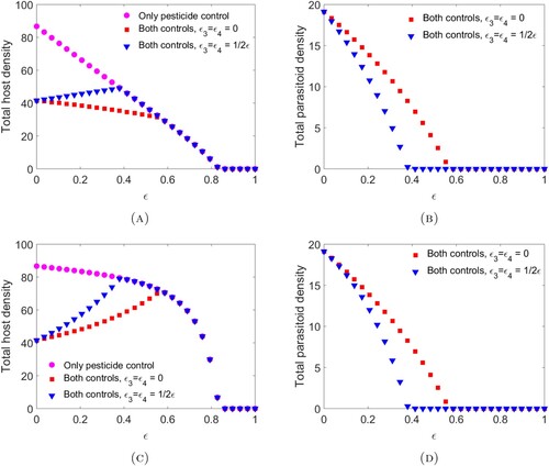All other parameters are fixed at the following values: $\begin{array}{rl}& f_0=400,s_1=0.1,s_2=0.1,{\gamma }_1=0.9,c=5,\\ & {\beta }_1=0.9,{\beta }_2=0.9,s_3=0.1,s_4=0.1,{\gamma }_3=0.3,a_1=1,a_2=1.\end{array}$For this choice of parameters, solutions are attracted to stable equilibria for all values of ϵ. Note that, in both cases, the parasitoid alone can never eradicate the host without additional parasitoid supplementation.

We observe that when spraying occurs at the end of the time interval (Figure 1A–B) and ${ϵ}_3={ϵ}_4=0$, then the combination of the two controls works are desired, with the total host abundance being lower than for chemical or biological control alone and the host going extinct for sufficiently large ϵ. Meanwhile, when the pesticide does result in direct mortality in the parasitoid, ${ϵ}_3={ϵ}_4=\frac{1}{2}ϵ$, then the host density experiences a moderate increase as ϵ increases but does not exceed the host density with only chemical control. Conversely, when spraying occurs at the beginning of the time unit (Figure 1C–D), then the combination of chemical and biological controls may produce a worse scenario than biological control alone. This occurs even when the chemical control has no direct effects on the parasitoid due to increased indirect mortality (refer to the equation for $P_1$ in model (11(11) $\begin{array}{rl}{H}_1(t+1)& =f((1-{ϵ}_2)H_2(t))(1-{ϵ}_2)H_2(t)e^{-a_2(1-{ϵ}_4)P_2(t)}\\ & +s_1(1-{\gamma }_1)(1-{ϵ}_1)H_1(t)e^{-a_1(1-{ϵ}_4)P_2(t)},\\ H_2(t+1)& =s_1{\gamma }_1(1-{ϵ}_1)H_1(t)e^{-a_1(1-{ϵ}_4)P_2(t)}\\ & +s_2(1-{ϵ}_2)H_2(t)e^{-a_2(1-{ϵ}_4)P_2(t)},\\ P_1(t+1)& ={\beta }_1(1-{ϵ}_1)H_1(t)(1-e^{-a_1(1-{ϵ}_4)P_2(t)})\\ & +{\beta }_2(1-{ϵ}_2)H_2(t)(1-e^{-a_2(1-{ϵ}_4)P_2(t)})\\ & +s_3(1-{\gamma }_3)(1-{ϵ}_3)P_1(t),\\ P_2(t+1)& =s_3{\gamma }_3(1-{ϵ}_3)P_1(t)+s_4(1-{ϵ}_4)P_2(t).\end{array}$(11) )).

Figure 1. The bifurcation diagrams for pesticide spraying at the end of the time unit (A)–(B) and pesticide spraying at the beginning of the time unit (C)–(D). These diagrams were obtained by finding the time-series solution out to time 20,000 for initial conditions $H_1(0)=H_2(0)=P_1(0)=P_2(0)=1$ using parameter values provided in Example 3.10. We consider three cases: only chemical controls are applied ($P_1(t)\equiv P_2(t)\equiv 0$) (magenta circle), both chemical and biological controls are applied with no direct effects on the parasitoid (${ϵ}_3={ϵ}_4=0$) (red square), and both chemical and biological controls are applied with direct effects on the parasitoid (${ϵ}_3={ϵ}_4=\frac{1}{2}ϵ$) (blue triangle).

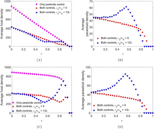
However, when parameter values are chosen so that the model exhibits oscillatory behaviour, this pattern can change. This is illustrated in Figure 2 where all parameters are the same as in Figure 1 except for host fecundity which has been increase to $f_0=4,000$. This increase in $f_0$ results in stable oscillatory dynamics for smaller values of ϵ. Specifically, for ${ϵ}_3={ϵ}_4=0$ these oscillations occur in both cases when $ϵ<0.764$ and for ${ϵ}_3={ϵ}_4=\frac{1}{2}ϵ$ these oscillations occur in both cases when $ϵ<0.819$. We observe that increasing ϵ within the oscillatory region may result in an increase in parasitoid abundance and a subsequent decrease in host abundance when the pesticide has direct mortality effects on the parasitoid.

Figure 2. The bifurcation diagrams for pesticide spraying at the end of the time unit (A)–(B) and pesticide spraying at the beginning of the time unit (C)–(D). These diagrams were obtained by finding the time-series solution out to time 20,000 for initial conditions $H_1(0)=H_2(0)=P_1(0)=P_2(0)=1$ using parameter values provided in Example 3.10 except with host fecundity increased to $f_0=4000$. We then plot the average host and parasitoid densities using the last 500 time units. We consider three cases: only chemical controls are applied ($P_1(t)\equiv P_2(t)\equiv 0$) (magenta circle), both chemical and biological controls are applied with no direct effects on the parasitoid (${ϵ}_3={ϵ}_4=0$) (red square), and both chemical and biological controls are applied with direct effects on the parasitoid (${ϵ}_3={ϵ}_4=\frac{1}{2}ϵ$) (blue triangle).

4. Host–parasitoid model with periodic impulsive effects

In Section 3.3, we observed that with continuous control it is possible for the combination of chemical control and natural enemies to produce worse outcomes in terms of host control than natural enemies alone if the chemical control is not sufficiently effective. However, more realistically we may expect chemical controls to be applied periodically rather than continuously. In this section, we extend model (1(1) $\begin{array}{rl}{H}_1(t+1)& =f(H_2(t))H_2(t)e^{-a_2{P}_2(t)}+s_1(1-{\gamma }_1)H_1(t)e^{-a_1{P}_2(t)},\\ H_2(t+1)& =s_1{\gamma }_1{H}_1(t)e^{-a_1{P}_2(t)}+s_2{H}_2(t)e^{-a_2{P}_2(t)},\\ P_1(t+1)& ={\beta }_1{H}_1(t)(1-e^{-a_1{P}_2(t)})+{\beta }_2{H}_2(t)(1-e^{-a_2{P}_2(t)})\\ & +s_3(1-{\gamma }_3)P_1(t),\\ P_2(t+1)& =s_3{\gamma }_3{P}_1(t)+s_4{P}_2(t),\end{array}$(1) ) to an impulsive difference equation that includes periodic pesticide spraying along with periodic releases of parasitoids. This extension is obtained by following a model formulation similar to that studied in [39].

We assume that at every qth time step there is a perturbation which incorporates a proportional decrease of the host and parasitoid population due to the application of pesticides and an increase of the parasitoid population due to the release of a constant number of parasitoids which is independent of the current parasitoid density. This perturbation is assumed to occur at the end of the time unit. The model is given by following system of difference equations: (12) $\begin{array}{rl}{H}_1(t+1)& =f(H_2(t))H_2(t)e^{-a_2{P}_2(t)}+s_1(1-{\gamma }_1)H_1(t)e^{-a_1{P}_2(t)},\\ H_2(t+1)& =s_1{\gamma }_1{H}_1(t)e^{-a_1{P}_2(t)}+s_2{H}_2(t)e^{-a_2{P}_2(t)},\\ P_1(t+1)& ={\beta }_1{H}_1(t)(1-e^{-a_1{P}_2(t)})+{\beta }_2{H}_2(t)(1-e^{-a_2{P}_2(t)})\\ & +s_3(1-{\gamma }_3)P_1(t),\\ P_2(t+1)& =s_3{\gamma }_3{P}_1(t)+s_4{P}_2(t),\\ H_1(q{k}^{+})& =(1-{ϵ}_1)H_1(qk),\\ H_2(q{k}^{+})& =(1-{ϵ}_2)H_2(qk),\\ P_1(q{k}^{+})& =(1-{ϵ}_3)P_1(qk)+{\tau }_1,\\ P_2(q{k}^{+})& =(1-{ϵ}_4)P_2(qk)+{\tau }_2,\end{array}$(12) where q is a fixed integer and denotes the period of the impulsive effect, which means that an integrated control strategy is applied during time unit t = qk for $k=1,2,\dots$. Here ${ϵ}_i$, $0\le {ϵ}_i\le 1$, for i = 1, 2, 3, 4 denotes the proportion of individuals in each stage that die as a result of pesticide spraying at time qk, and ${\tau }_i\ge 0$ for i = 1, 2 gives the amount of juvenile and adult parasitoids that are released at this time. $H_i(qk)$ and $P_i(qk)$ for i = 1, 2 are the densities of the host and parasitoid, respectively, at time qk prior to the impulsive perturbation, and $H_i(q{k}^{+})$ and $P_i(q{k}^{+})$ are the densities of host and parasitoid at time qk after an impulsive perturbation. The initial conditions are $(H_1(0^{+}),H_2(0^{+}),P_1(0^{+}),P_2(0^{+}))=(H_1(0),H_2(0),P_1(0),P_2(0))$. Here for convenience we denote the initial density after an impulsive perturbation at time t = 0.

Note that if q = 1 and ${\tau }_1={\tau }_2=0$, then system (12(12) $\begin{array}{rl}{H}_1(t+1)& =f(H_2(t))H_2(t)e^{-a_2{P}_2(t)}+s_1(1-{\gamma }_1)H_1(t)e^{-a_1{P}_2(t)},\\ H_2(t+1)& =s_1{\gamma }_1{H}_1(t)e^{-a_1{P}_2(t)}+s_2{H}_2(t)e^{-a_2{P}_2(t)},\\ P_1(t+1)& ={\beta }_1{H}_1(t)(1-e^{-a_1{P}_2(t)})+{\beta }_2{H}_2(t)(1-e^{-a_2{P}_2(t)})\\ & +s_3(1-{\gamma }_3)P_1(t),\\ P_2(t+1)& =s_3{\gamma }_3{P}_1(t)+s_4{P}_2(t),\\ H_1(q{k}^{+})& =(1-{ϵ}_1)H_1(qk),\\ H_2(q{k}^{+})& =(1-{ϵ}_2)H_2(qk),\\ P_1(q{k}^{+})& =(1-{ϵ}_3)P_1(qk)+{\tau }_1,\\ P_2(q{k}^{+})& =(1-{ϵ}_4)P_2(qk)+{\tau }_2,\end{array}$(12) ) is equivalent to continuous spraying at the end of the time interval, as given by system (10(10) $\begin{array}{rl}{H}_1(t+1)& =[f(H_2(t))H_2(t)e^{-a_2{P}_2(t)}+s_1(1-{\gamma }_1)H_1(t)e^{-a_1{P}_2(t)}](1-{ϵ}_1),\\ H_2(t+1)& =[s_1{\gamma }_1{H}_1(t)e^{-a_1{P}_2(t)}+s_2{H}_2(t)e^{-a_2{P}_2(t)}](1-{ϵ}_2),\\ P_1(t+1)& =[{\beta }_1{H}_1(t)(1-e^{-a_1{P}_2(t)})+{\beta }_2{H}_2(t)(1-e^{-a_2{P}_2(t)})\\ & +s_3(1-{\gamma }_3)P_1(t)](1-{ϵ}_3),\\ P_2(t+1)& =[s_3{\gamma }_3{P}_1(t)+s_4{P}_2(t)](1-{ϵ}_4).\end{array}$(10) ).

4.1. Host-eradication periodic solutions

Our goal is to determine when system (12(12) $\begin{array}{rl}{H}_1(t+1)& =f(H_2(t))H_2(t)e^{-a_2{P}_2(t)}+s_1(1-{\gamma }_1)H_1(t)e^{-a_1{P}_2(t)},\\ H_2(t+1)& =s_1{\gamma }_1{H}_1(t)e^{-a_1{P}_2(t)}+s_2{H}_2(t)e^{-a_2{P}_2(t)},\\ P_1(t+1)& ={\beta }_1{H}_1(t)(1-e^{-a_1{P}_2(t)})+{\beta }_2{H}_2(t)(1-e^{-a_2{P}_2(t)})\\ & +s_3(1-{\gamma }_3)P_1(t),\\ P_2(t+1)& =s_3{\gamma }_3{P}_1(t)+s_4{P}_2(t),\\ H_1(q{k}^{+})& =(1-{ϵ}_1)H_1(qk),\\ H_2(q{k}^{+})& =(1-{ϵ}_2)H_2(qk),\\ P_1(q{k}^{+})& =(1-{ϵ}_3)P_1(qk)+{\tau }_1,\\ P_2(q{k}^{+})& =(1-{ϵ}_4)P_2(qk)+{\tau }_2,\end{array}$(12) ) results in host eradication. To this end, we first establish the existence of host-eradication periodic solutions. Consider the parasitoid-only subsystem of model (12(12) $\begin{array}{rl}{H}_1(t+1)& =f(H_2(t))H_2(t)e^{-a_2{P}_2(t)}+s_1(1-{\gamma }_1)H_1(t)e^{-a_1{P}_2(t)},\\ H_2(t+1)& =s_1{\gamma }_1{H}_1(t)e^{-a_1{P}_2(t)}+s_2{H}_2(t)e^{-a_2{P}_2(t)},\\ P_1(t+1)& ={\beta }_1{H}_1(t)(1-e^{-a_1{P}_2(t)})+{\beta }_2{H}_2(t)(1-e^{-a_2{P}_2(t)})\\ & +s_3(1-{\gamma }_3)P_1(t),\\ P_2(t+1)& =s_3{\gamma }_3{P}_1(t)+s_4{P}_2(t),\\ H_1(q{k}^{+})& =(1-{ϵ}_1)H_1(qk),\\ H_2(q{k}^{+})& =(1-{ϵ}_2)H_2(qk),\\ P_1(q{k}^{+})& =(1-{ϵ}_3)P_1(qk)+{\tau }_1,\\ P_2(q{k}^{+})& =(1-{ϵ}_4)P_2(qk)+{\tau }_2,\end{array}$(12) ): (13) $\begin{array}{rl}{P}_1(t+1)& =s_3(1-{\gamma }_3)P_1(t),\\ P_2(t+1)& =s_3{\gamma }_3{P}_1(t)+s_4{P}_2(t),\\ P_1(q{k}^{+})& =(1-{ϵ}_3)P_1(qk)+{\tau }_1,\\ P_2(q{k}^{+})& =(1-{ϵ}_4)P_2(qk)+{\tau }_2,\\ P_1(0^{+})& =P_1(0),\\ P_2(0^{+})& =P_2(0).\end{array}$(13) In Lemma 4.1, we show that all solutions of system (13(13) $\begin{array}{rl}{P}_1(t+1)& =s_3(1-{\gamma }_3)P_1(t),\\ P_2(t+1)& =s_3{\gamma }_3{P}_1(t)+s_4{P}_2(t),\\ P_1(q{k}^{+})& =(1-{ϵ}_3)P_1(qk)+{\tau }_1,\\ P_2(q{k}^{+})& =(1-{ϵ}_4)P_2(qk)+{\tau }_2,\\ P_1(0^{+})& =P_1(0),\\ P_2(0^{+})& =P_2(0).\end{array}$(13) ) converge to a positive periodic solution.

Lemma 4.1

System (13(13) $\begin{array}{rl}{P}_1(t+1)& =s_3(1-{\gamma }_3)P_1(t),\\ P_2(t+1)& =s_3{\gamma }_3{P}_1(t)+s_4{P}_2(t),\\ P_1(q{k}^{+})& =(1-{ϵ}_3)P_1(qk)+{\tau }_1,\\ P_2(q{k}^{+})& =(1-{ϵ}_4)P_2(qk)+{\tau }_2,\\ P_1(0^{+})& =P_1(0),\\ P_2(0^{+})& =P_2(0).\end{array}$(13) ) has a periodic solution $P_t^{\ast }$ defined as ${\left(\begin{array}{c}{P}_1\\ P_2\end{array}\right)}_t^{\ast }={\left(\begin{array}{cc}{s}_3(1-{\gamma }_3)& 0\\ s_3{\gamma }_3& s_4\end{array}\right)}^{t-qs}\left(\begin{array}{c}{P}_{1,0}\\ P_{2,0}\end{array}\right),$where $t\in [q{s}^{+},q(s+1)),s=0,1,2\cdots ,$ and $\left(\begin{array}{c}{P}_{1,0}\\ P_{2,0}\end{array}\right)=\left(\begin{array}{c}{\displaystyle \frac{{\tau }_1}{1-s_3^q(1-{ϵ}_3)(1-{\gamma }_3{)}^q}}\\ {\displaystyle \frac{s_3{\gamma }_3{\tau }_1(1-{ϵ}_4)\sum _{n=0}^{q-1}{s}_4^n(s_3(1-{\gamma }_3){)}^{q-1-n}}{(1-s_3^q(1-{\gamma }_3{)}^q(1-{ϵ}_3))(1-s_4^q(1-{ϵ}_4))}}+{\displaystyle \frac{{\tau }_2}{(1-s_4^q(1-{ϵ}_4))}}\end{array}\right).$Moreover, for every solution $P_t$ of (13(13) $\begin{array}{rl}{P}_1(t+1)& =s_3(1-{\gamma }_3)P_1(t),\\ P_2(t+1)& =s_3{\gamma }_3{P}_1(t)+s_4{P}_2(t),\\ P_1(q{k}^{+})& =(1-{ϵ}_3)P_1(qk)+{\tau }_1,\\ P_2(q{k}^{+})& =(1-{ϵ}_4)P_2(qk)+{\tau }_2,\\ P_1(0^{+})& =P_1(0),\\ P_2(0^{+})& =P_2(0).\end{array}$(13) ) we have $|P_t-P_t^{\ast }|\to 0$ as $t\to \mathrm{\infty }$.

Proof.

It follows from the periodicity of the system (13(13) $\begin{array}{rl}{P}_1(t+1)& =s_3(1-{\gamma }_3)P_1(t),\\ P_2(t+1)& =s_3{\gamma }_3{P}_1(t)+s_4{P}_2(t),\\ P_1(q{k}^{+})& =(1-{ϵ}_3)P_1(qk)+{\tau }_1,\\ P_2(q{k}^{+})& =(1-{ϵ}_4)P_2(qk)+{\tau }_2,\\ P_1(0^{+})& =P_1(0),\\ P_2(0^{+})& =P_2(0).\end{array}$(13) ) that the solution can be defined at the impulsive sub-interval $n\in [q{s}^{+},q(s+1))$ with $s=0,1,2\cdots$, where $n=q{s}^{+}$ means that we take the density of the parasitoid after an impulsive perturbation as the initial value in this interval. Initiating the population at time $q{s}^{+}$ and applying system (13(13) $\begin{array}{rl}{P}_1(t+1)& =s_3(1-{\gamma }_3)P_1(t),\\ P_2(t+1)& =s_3{\gamma }_3{P}_1(t)+s_4{P}_2(t),\\ P_1(q{k}^{+})& =(1-{ϵ}_3)P_1(qk)+{\tau }_1,\\ P_2(q{k}^{+})& =(1-{ϵ}_4)P_2(qk)+{\tau }_2,\\ P_1(0^{+})& =P_1(0),\\ P_2(0^{+})& =P_2(0).\end{array}$(13) ) we find that the solution at time $q(s+1)$ is given by ${\left(\begin{array}{c}{P}_1\\ P_2\end{array}\right)}_{q(s+1)}={\left(\begin{array}{cc}{s}_3(1-{\gamma }_3)& 0\\ s_3{\gamma }_3& s_4\end{array}\right)}^q{\left(\begin{array}{c}{P}_1\\ P_2\end{array}\right)}_{q{s}^{+}}.$Applying the impulsive condition we find (14) $\begin{array}{rl}{\left(\begin{array}{c}{P}_1\\ P_2\end{array}\right)}_{q(s+1{)}^{+}}& =\left(\begin{array}{cc}(1-{ϵ}_3)& 0\\ 0& (1-{ϵ}_4)\end{array}\right){\left(\begin{array}{c}{P}_1\\ P_2\end{array}\right)}_{q(s+1)}+\left(\begin{array}{c}{\tau }_1\\ {\tau }_2\end{array}\right)\\ & =\left(\begin{array}{cc}(1-{ϵ}_3)& 0\\ 0& (1-{ϵ}_4)\end{array}\right){\left(\begin{array}{cc}{s}_3(1-{\gamma }_3)& 0\\ s_3{\gamma }_3& s_4\end{array}\right)}^q{\left(\begin{array}{c}{P}_1\\ P_2\end{array}\right)}_{q{s}^{+}}+\left(\begin{array}{c}{\tau }_1\\ {\tau }_2\end{array}\right).\end{array}$(14) Therefore, the q-periodic solution of system (13(13) $\begin{array}{rl}{P}_1(t+1)& =s_3(1-{\gamma }_3)P_1(t),\\ P_2(t+1)& =s_3{\gamma }_3{P}_1(t)+s_4{P}_2(t),\\ P_1(q{k}^{+})& =(1-{ϵ}_3)P_1(qk)+{\tau }_1,\\ P_2(q{k}^{+})& =(1-{ϵ}_4)P_2(qk)+{\tau }_2,\\ P_1(0^{+})& =P_1(0),\\ P_2(0^{+})& =P_2(0).\end{array}$(13) ) is determined by the solution to the system $\left(\begin{array}{c}{P}_{1,0}\\ P_{2,0}\end{array}\right)=\left(\begin{array}{cc}{s}_3^q(1-{\gamma }_3{)}^q(1-{ϵ}_3)& 0\\ s_3{\gamma }_3(1-{ϵ}_4){\displaystyle \sum _{n=0}^{q-1}{s}_4^n(s_3(1-{\gamma }_3){)}^{q-1-n}}& s_4^q(1-{ϵ}_4)\end{array}\right)\left(\begin{array}{c}{P}_{1,0}\\ P_{2,0}\end{array}\right)+\left(\begin{array}{c}{\tau }_1\\ {\tau }_2\end{array}\right).$Solving this system we find $\begin{array}{rl}{P}_{1,0}& =\frac{{\tau }_1}{1-s_3^q(1-{\gamma }_3{)}^q(1-{ϵ}_3)},\\ P_{2,0}& =\frac{{\tau }_1{s}_3{\gamma }_3(1-{ϵ}_4)\sum _{n=0}^{q-1}{s}_4^n(s_3(1-{\gamma }_3){)}^{q-1-n}}{(1-s_3^q(1-{\gamma }_3{)}^q(1-{ϵ}_3))(1-s_4^q(1-{ϵ}_4))}+\frac{{\tau }_2}{(1-s_4^q(1-{ϵ}_4))}.\end{array}$Note that the restrictions on the model parameters ensure that these two quantities are always positive.

Next, we note that the convergence of solutions to the periodic solution $P_t^{\ast }$ follows from the linearity of the projection matrix in Equation (14(14) $\begin{array}{rl}{\left(\begin{array}{c}{P}_1\\ P_2\end{array}\right)}_{q(s+1{)}^{+}}& =\left(\begin{array}{cc}(1-{ϵ}_3)& 0\\ 0& (1-{ϵ}_4)\end{array}\right){\left(\begin{array}{c}{P}_1\\ P_2\end{array}\right)}_{q(s+1)}+\left(\begin{array}{c}{\tau }_1\\ {\tau }_2\end{array}\right)\\ & =\left(\begin{array}{cc}(1-{ϵ}_3)& 0\\ 0& (1-{ϵ}_4)\end{array}\right){\left(\begin{array}{cc}{s}_3(1-{\gamma }_3)& 0\\ s_3{\gamma }_3& s_4\end{array}\right)}^q{\left(\begin{array}{c}{P}_1\\ P_2\end{array}\right)}_{q{s}^{+}}+\left(\begin{array}{c}{\tau }_1\\ {\tau }_2\end{array}\right).\end{array}$(14) ) and the fact that the eigenvalues of this matrix have absolute values less than 1. Specifically, define $\begin{array}{rl}{A}_p& :=\left(\begin{array}{cc}{s}_3^q(1-{\gamma }_3{)}^q(1-{ϵ}_3)& 0\\ s_3{\gamma }_3(1-{ϵ}_4){\displaystyle \sum _{n=0}^{q-1}{s}_4^n(s_3(1-{\gamma }_3){)}^{q-1-n}}& s_4^q(1-{ϵ}_4)\end{array}\right),\\ P& :=\left(\begin{array}{c}{P}_1\\ P_2\end{array}\right),\mathrm{and}\tau :=\left(\begin{array}{c}{\tau }_1\\ {\tau }_2\end{array}\right).\end{array}$Then iterating Equation (14(14) $\begin{array}{rl}{\left(\begin{array}{c}{P}_1\\ P_2\end{array}\right)}_{q(s+1{)}^{+}}& =\left(\begin{array}{cc}(1-{ϵ}_3)& 0\\ 0& (1-{ϵ}_4)\end{array}\right){\left(\begin{array}{c}{P}_1\\ P_2\end{array}\right)}_{q(s+1)}+\left(\begin{array}{c}{\tau }_1\\ {\tau }_2\end{array}\right)\\ & =\left(\begin{array}{cc}(1-{ϵ}_3)& 0\\ 0& (1-{ϵ}_4)\end{array}\right){\left(\begin{array}{cc}{s}_3(1-{\gamma }_3)& 0\\ s_3{\gamma }_3& s_4\end{array}\right)}^q{\left(\begin{array}{c}{P}_1\\ P_2\end{array}\right)}_{q{s}^{+}}+\left(\begin{array}{c}{\tau }_1\\ {\tau }_2\end{array}\right).\end{array}$(14) ), we obtain $P(q(s+1{)}^{+})=A_p^{(s+1)}P(0)+\sum _{i=0}^s{A}_p^{s-i}\tau .$Since $\rho [A_p]<1$, taking the limit as $s\to \mathrm{\infty }$ we find that the solution converges to $(I-A_p{)}^{-1}\tau$ which is the equilibrium solution to Equation (14(14) $\begin{array}{rl}{\left(\begin{array}{c}{P}_1\\ P_2\end{array}\right)}_{q(s+1{)}^{+}}& =\left(\begin{array}{cc}(1-{ϵ}_3)& 0\\ 0& (1-{ϵ}_4)\end{array}\right){\left(\begin{array}{c}{P}_1\\ P_2\end{array}\right)}_{q(s+1)}+\left(\begin{array}{c}{\tau }_1\\ {\tau }_2\end{array}\right)\\ & =\left(\begin{array}{cc}(1-{ϵ}_3)& 0\\ 0& (1-{ϵ}_4)\end{array}\right){\left(\begin{array}{cc}{s}_3(1-{\gamma }_3)& 0\\ s_3{\gamma }_3& s_4\end{array}\right)}^q{\left(\begin{array}{c}{P}_1\\ P_2\end{array}\right)}_{q{s}^{+}}+\left(\begin{array}{c}{\tau }_1\\ {\tau }_2\end{array}\right).\end{array}$(14) ).

Next, in Theorem 4.2 we establish sufficient conditions under which a given control strategy results in host eradication.

Theorem 4.2

The host-eradication cycle $(0,0,P_{1,t}^{\ast },P_{2,t}^{\ast })$ is a globally attracting solution of system (12(12) $\begin{array}{rl}{H}_1(t+1)& =f(H_2(t))H_2(t)e^{-a_2{P}_2(t)}+s_1(1-{\gamma }_1)H_1(t)e^{-a_1{P}_2(t)},\\ H_2(t+1)& =s_1{\gamma }_1{H}_1(t)e^{-a_1{P}_2(t)}+s_2{H}_2(t)e^{-a_2{P}_2(t)},\\ P_1(t+1)& ={\beta }_1{H}_1(t)(1-e^{-a_1{P}_2(t)})+{\beta }_2{H}_2(t)(1-e^{-a_2{P}_2(t)})\\ & +s_3(1-{\gamma }_3)P_1(t),\\ P_2(t+1)& =s_3{\gamma }_3{P}_1(t)+s_4{P}_2(t),\\ H_1(q{k}^{+})& =(1-{ϵ}_1)H_1(qk),\\ H_2(q{k}^{+})& =(1-{ϵ}_2)H_2(qk),\\ P_1(q{k}^{+})& =(1-{ϵ}_3)P_1(qk)+{\tau }_1,\\ P_2(q{k}^{+})& =(1-{ϵ}_4)P_2(qk)+{\tau }_2,\end{array}$(12) ) if (15) $\rho \left[\prod _{t=qs}^{q(s+1)-1}\left(\begin{array}{cc}{s}_1(1-{\gamma }_1)e^{-a_1{P}_2^{\ast }(t)}& f(0)e^{-a_2{P}_2^{\ast }(t)}\\ s_1{\gamma }_1{e}^{-a_1{P}_2^{\ast }(t)}& s_2{e}^{-a_2{P}_2^{\ast }(t)}\end{array}\right)\right]<1.$(15) In particular, a sufficient condition is (16) ${\lambda }^q(1-min\{{ϵ}_1,{ϵ}_2\})\prod _{t=qs}^{q(s+1)-1}{e}^{-min\{a_1,a_2\}{P}_2^{\ast }(t)}<1,$(16) where $\lambda :=\rho [A_h(0,0,0,0)].$

Proof.

Note that $\begin{array}{rl}{P}_1(t+1)& \ge s_3(1-{\gamma }_3)P_1(t),\\ P_2(t+1)& \ge s_3{\gamma }_3{P}_1(t)+s_4{P}_2(t).\end{array}$Consider the following impulsive difference equation: (17) $\begin{array}{rl}& Q_1(t+1)=s_3(1-{\gamma }_3)Q_1(t),\\ & Q_2(t+1)=s_3{\gamma }_3{Q}_1(t)+s_4{Q}_2(t),\\ & Q_1(q{k}^{+})=(1-{ϵ}_3)Q_1(qk)+{\tau }_1,\\ & Q_2(q{k}^{+})=(1-{ϵ}_4)Q_2(qk)+{\tau }_2,\end{array}$(17) where $n=0,1,2,\dots$ and $k=1,2,\dots$ It follows from Lemma 4.1 that if $P_1(0)=Q_1(0)$ and $P_2(0)=Q_2(0)$, then we have $P_1(t)\ge Q_1(t)$ and $P_2(t)\ge Q_2(t)$ and $Q_1(t)\to P_1^{\ast }(t)$ and $Q_2(t)\to P_2^{\ast }(t)$ as $t\to \mathrm{\infty }.$ Hence, for any $\delta >0$ there exists $t_0>0$ such that $P_1(t)\ge Q_1(t)>P_1^{\ast }(t)-\delta$ and $P_2(t)\ge Q_2(t)>P_2^{\ast }(t)-\delta$ for $t\ge t_0$. Therefore, for $t\ge t_0$ we have (18) $\begin{array}{rl}{H}_1(t+1)& \le f(H_2(t))H_2(t)e^{-a_2(P_2^{\ast }(t)-\delta )}+s_1(1-{\gamma }_1)H_1(t)e^{-a_1(P_2^{\ast }(t)-\delta )},\\ H_2(t+1)& \le s_1{\gamma }_1{H}_1(t)e^{-a_1(P_2^{\ast }(t)-\delta )}+s_2{H}_2(t)e^{-a_2(P_2^{\ast }(t)-\delta )},\\ H_1(q{k}^{+})& =(1-{ϵ}_1)H_1(qk),\\ H_2(q{k}^{+})& =(1-{ϵ}_2)H_2(qk).\end{array}$(18) It follows that $\begin{array}{rl}{\left(\begin{array}{c}{H}_1\\ H_2\end{array}\right)}_{q(s+1)}& \le \prod _{t=qs}^{q(s+1)-1}\left(\begin{array}{cc}{s}_1(1-{\gamma }_1)e^{-a_1(P_2^{\ast }(t)-\delta )}& f(H_2(t))e^{-a_2(P_2^{\ast }(t)-\delta )}\\ s_1{\gamma }_1{e}^{-a_1(P_2^{\ast }(t)-\delta )}& s_2{e}^{-a_2(P_2^{\ast }(t)-\delta )}\end{array}\right){\left(\begin{array}{c}{H}_1\\ H_2\end{array}\right)}_{q{s}^{+}}\\ & \le \prod _{t=qs}^{q(s+1)-1}\left(\begin{array}{cc}{s}_1(1-{\gamma }_1)e^{-a_1{P}_2^{\ast }(t)}& f(0)e^{-a_2{P}_2^{\ast }(t)}\\ s_1{\gamma }_1{e}^{-a_1{P}_2^{\ast }(t)}& s_2{e}^{-a_2{P}_2^{\ast }(t)}\end{array}\right){\left(\begin{array}{c}{H}_1\\ H_2\end{array}\right)}_{q{s}^{+}}.\end{array}$Thus, if inequality (15(15) $\rho \left[\prod _{t=qs}^{q(s+1)-1}\left(\begin{array}{cc}{s}_1(1-{\gamma }_1)e^{-a_1{P}_2^{\ast }(t)}& f(0)e^{-a_2{P}_2^{\ast }(t)}\\ s_1{\gamma }_1{e}^{-a_1{P}_2^{\ast }(t)}& s_2{e}^{-a_2{P}_2^{\ast }(t)}\end{array}\right)\right]<1.$(15) ) is satisfied, then $H_{1,qs}\to 0$, $H_{2,qs}\to 0$ as $s\to \mathrm{\infty }.$ Consequently, $H_1\to 0$ and $H_2\to 0$ as $t\to \mathrm{\infty }.$

The sufficient condition for (15(15) $\rho \left[\prod _{t=qs}^{q(s+1)-1}\left(\begin{array}{cc}{s}_1(1-{\gamma }_1)e^{-a_1{P}_2^{\ast }(t)}& f(0)e^{-a_2{P}_2^{\ast }(t)}\\ s_1{\gamma }_1{e}^{-a_1{P}_2^{\ast }(t)}& s_2{e}^{-a_2{P}_2^{\ast }(t)}\end{array}\right)\right]<1.$(15) ) can be obtained by noting that $\begin{array}{rl}{\left(\begin{array}{c}{H}_1\\ H_2\end{array}\right)}_{q(s+1)}& \le {\left(\begin{array}{cc}{s}_1(1-{\gamma }_1)& f(0)\\ s_1{\gamma }_1& s_2\end{array}\right)}^q\left(\begin{array}{cc}(1-{ϵ}_1)& 0\\ 0& (1-{ϵ}_2)\end{array}\right)\\ & \times \prod _{t=qs}^{q(s+1)-1}{e}^{-min\{a_1,a_2\}{P}_2^{\ast }(t)}{\left(\begin{array}{c}{H}_1\\ H_2\end{array}\right)}_{qs}.\end{array}$

4.2. Numerical study of the impulsive model

In this section, we further study the dynamics of the impulsive model (12(12) $\begin{array}{rl}{H}_1(t+1)& =f(H_2(t))H_2(t)e^{-a_2{P}_2(t)}+s_1(1-{\gamma }_1)H_1(t)e^{-a_1{P}_2(t)},\\ H_2(t+1)& =s_1{\gamma }_1{H}_1(t)e^{-a_1{P}_2(t)}+s_2{H}_2(t)e^{-a_2{P}_2(t)},\\ P_1(t+1)& ={\beta }_1{H}_1(t)(1-e^{-a_1{P}_2(t)})+{\beta }_2{H}_2(t)(1-e^{-a_2{P}_2(t)})\\ & +s_3(1-{\gamma }_3)P_1(t),\\ P_2(t+1)& =s_3{\gamma }_3{P}_1(t)+s_4{P}_2(t),\\ H_1(q{k}^{+})& =(1-{ϵ}_1)H_1(qk),\\ H_2(q{k}^{+})& =(1-{ϵ}_2)H_2(qk),\\ P_1(q{k}^{+})& =(1-{ϵ}_3)P_1(qk)+{\tau }_1,\\ P_2(q{k}^{+})& =(1-{ϵ}_4)P_2(qk)+{\tau }_2,\end{array}$(12) ). In Example 4.3, we first consider the impact of combined control strategies, i.e. chemical and biological control, when controls are applied periodically. Next, in Example 4.4 consider how host density varies for differing control strategies in the case when host eradication is not achieved. We find that there are parameter ranges for which multiple attractors occur and, thus, the effectiveness of control is initial condition dependent.

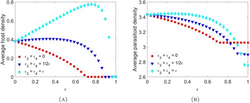
Example 4.3

Interaction of control strategies in the impulsive model

We consider the impact of varying the pesticide-induced mortality in the host assuming equal impacts on both stages, i.e. ${ϵ}_1={ϵ}_2=ϵ$. We consider three scenarios: pesticide spraying does not directly impact the parasitoid (${ϵ}_3={ϵ}_4=0$), has moderate impacts on the parasitoid (${ϵ}_3={ϵ}_4=\frac{1}{2}ϵ$) or has severe impacts on the parasitoid (${ϵ}_3={ϵ}_4=ϵ$). All other parameters are fixed at the following values: $\begin{array}{rl}& f_0=500,s_1=0.71,s_2=0.71,{\gamma }_1=0.93,c=5,\\ & {\beta }_1=0.3,{\beta }_2=0.3,s_3=0.71,s_4=0.72,{\gamma }_3=0.25,a_1=1,a_2=1,\\ & q=7,{\tau }_1=1,{\tau }_2=5.\end{array}$We observe that when there are no direct mortality effects on the parasitoid, then the average host density is a decreasing function of the toxicant effect ϵ (Figure 3A). Since the impulsive model corresponds to spraying at the end of the time unit, this is in agreement with the dynamics observed in Example 3.10 (Figure 1A). Meanwhile, when direct effects on the parasitoid are present we again observe that the average host density can increase with increasing pesticide concentration resulting in host densities almost doubling in certain situations. Note here that, due to parasitoid supplementation, the parasitoid population survives even when the hosts die out (Figure 3B). Also note that, similar to the case where models (10(10) $\begin{array}{rl}{H}_1(t+1)& =[f(H_2(t))H_2(t)e^{-a_2{P}_2(t)}+s_1(1-{\gamma }_1)H_1(t)e^{-a_1{P}_2(t)}](1-{ϵ}_1),\\ H_2(t+1)& =[s_1{\gamma }_1{H}_1(t)e^{-a_1{P}_2(t)}+s_2{H}_2(t)e^{-a_2{P}_2(t)}](1-{ϵ}_2),\\ P_1(t+1)& =[{\beta }_1{H}_1(t)(1-e^{-a_1{P}_2(t)})+{\beta }_2{H}_2(t)(1-e^{-a_2{P}_2(t)})\\ & +s_3(1-{\gamma }_3)P_1(t)](1-{ϵ}_3),\\ P_2(t+1)& =[s_3{\gamma }_3{P}_1(t)+s_4{P}_2(t)](1-{ϵ}_4).\end{array}$(10) ) and (11(11) $\begin{array}{rl}{H}_1(t+1)& =f((1-{ϵ}_2)H_2(t))(1-{ϵ}_2)H_2(t)e^{-a_2(1-{ϵ}_4)P_2(t)}\\ & +s_1(1-{\gamma }_1)(1-{ϵ}_1)H_1(t)e^{-a_1(1-{ϵ}_4)P_2(t)},\\ H_2(t+1)& =s_1{\gamma }_1(1-{ϵ}_1)H_1(t)e^{-a_1(1-{ϵ}_4)P_2(t)}\\ & +s_2(1-{ϵ}_2)H_2(t)e^{-a_2(1-{ϵ}_4)P_2(t)},\\ P_1(t+1)& ={\beta }_1(1-{ϵ}_1)H_1(t)(1-e^{-a_1(1-{ϵ}_4)P_2(t)})\\ & +{\beta }_2(1-{ϵ}_2)H_2(t)(1-e^{-a_2(1-{ϵ}_4)P_2(t)})\\ & +s_3(1-{\gamma }_3)(1-{ϵ}_3)P_1(t),\\ P_2(t+1)& =s_3{\gamma }_3(1-{ϵ}_3)P_1(t)+s_4(1-{ϵ}_4)P_2(t).\end{array}$(11) ) exhibit oscillatory dynamics (Figure 2), it is possible for parasitoid densities to be higher when they experience greater pesticide mortality.

Figure 3. The bifurcation diagrams for the impulsive system (12(12) $\begin{array}{rl}{H}_1(t+1)& =f(H_2(t))H_2(t)e^{-a_2{P}_2(t)}+s_1(1-{\gamma }_1)H_1(t)e^{-a_1{P}_2(t)},\\ H_2(t+1)& =s_1{\gamma }_1{H}_1(t)e^{-a_1{P}_2(t)}+s_2{H}_2(t)e^{-a_2{P}_2(t)},\\ P_1(t+1)& ={\beta }_1{H}_1(t)(1-e^{-a_1{P}_2(t)})+{\beta }_2{H}_2(t)(1-e^{-a_2{P}_2(t)})\\ & +s_3(1-{\gamma }_3)P_1(t),\\ P_2(t+1)& =s_3{\gamma }_3{P}_1(t)+s_4{P}_2(t),\\ H_1(q{k}^{+})& =(1-{ϵ}_1)H_1(qk),\\ H_2(q{k}^{+})& =(1-{ϵ}_2)H_2(qk),\\ P_1(q{k}^{+})& =(1-{ϵ}_3)P_1(qk)+{\tau }_1,\\ P_2(q{k}^{+})& =(1-{ϵ}_4)P_2(qk)+{\tau }_2,\end{array}$(12) ). These diagrams were obtained by finding the time-series solution out to time 5000 for initial conditions $H_1(0)=H_2(0)=P_1(0)=P_2(0)=1$ using parameter values provided in Example 4.3. We then plot the average host and parasitoid densities using the last 500 time units. We consider three cases: no direct effects on the parasitoid (${ϵ}_3={ϵ}_4=0$) (red square), moderate direct effects on the parasitoid (${ϵ}_3={ϵ}_4=\frac{1}{2}ϵ$) (blue triangle) and severe direct effects on the parasitoid (${ϵ}_3={ϵ}_4=ϵ$) (cyan diamond).

Example 4.4

Impact of control strategies on host densities

In this example, we first consider the impact of varying the control parameters q and ${\tau }_2$. We fix all other parameters at the following values: $\begin{array}{rl}& f_0=140,s_1=0.11,s_2=0.11,{\gamma }_1=0.13,c=0.8,\\ & {\beta }_1=1.3,{\beta }_2=1.8,s_3=0.54,s_4=0.83,{\gamma }_3=0.25,a_1=0.1,a_2=0.1,\\ & {ϵ}_1=0.18,{ϵ}_2=0.17,{ϵ}_3=0.15,{ϵ}_4=0.15,{\tau }_1=5.\end{array}$In Figure 4(A), we give the average host density against the control frequency q and the number of adult parasitoids released ${\tau }_2$. 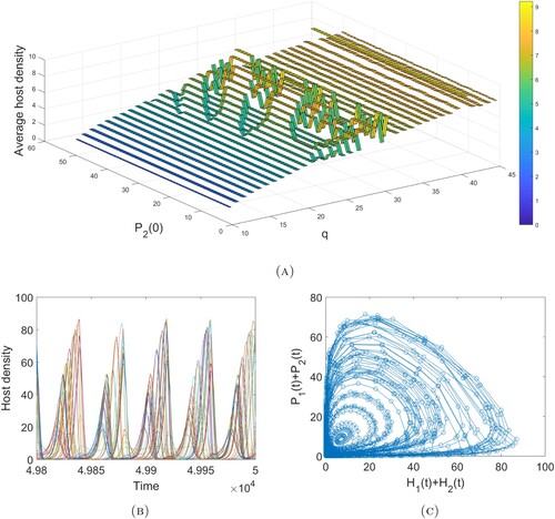We observe that the host is eradicated for sufficiently strong control measures (i.e. high frequency pesticide spraying and/or a large parasitoid release number), while its average density follows a generally increasing trend as these control measures are weakened. However, there are parameter regions for which this increasing trend does not hold. This is a result of the existence of multiple stable attractors with significant differences in average host densities in certain regions (Figure 4B). 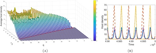To examine this phenomenon further, we fix ${\tau }_2=4$ and find the average host density against q and $P_2(0)$ (Figure 5A). We observe a region of intermediate q values for which these multi-attractors produce noticeable changes in host densities. Investigation of the larger q parameter space shows that though changes in host density are not as significant, the system dynamics are quite complicated and exhibit a large numbers of attractors (Figure 5B–C).

Figure 4. (A) The average host density against q and ${\tau }_2$ obtained from the last 100,000 values of a 500,000 time unit simulation. All parameters are as given in Example 4.4 and initial conditions are $H_1(0)=H_2(0)=P_1(0)=P_2(0)=1$. The red line corresponds to the host eradication condition (16(16) ${\lambda }^q(1-min\{{ϵ}_1,{ϵ}_2\})\prod _{t=qs}^{q(s+1)-1}{e}^{-min\{a_1,a_2\}{P}_2^{\ast }(t)}<1,$(16) ). Note that q must be integer-valued. (B) The final time solutions of system (12(12) $\begin{array}{rl}{H}_1(t+1)& =f(H_2(t))H_2(t)e^{-a_2{P}_2(t)}+s_1(1-{\gamma }_1)H_1(t)e^{-a_1{P}_2(t)},\\ H_2(t+1)& =s_1{\gamma }_1{H}_1(t)e^{-a_1{P}_2(t)}+s_2{H}_2(t)e^{-a_2{P}_2(t)},\\ P_1(t+1)& ={\beta }_1{H}_1(t)(1-e^{-a_1{P}_2(t)})+{\beta }_2{H}_2(t)(1-e^{-a_2{P}_2(t)})\\ & +s_3(1-{\gamma }_3)P_1(t),\\ P_2(t+1)& =s_3{\gamma }_3{P}_1(t)+s_4{P}_2(t),\\ H_1(q{k}^{+})& =(1-{ϵ}_1)H_1(qk),\\ H_2(q{k}^{+})& =(1-{ϵ}_2)H_2(qk),\\ P_1(q{k}^{+})& =(1-{ϵ}_3)P_1(qk)+{\tau }_1,\\ P_2(q{k}^{+})& =(1-{ϵ}_4)P_2(qk)+{\tau }_2,\end{array}$(12) ) when q = 30 and ${\tau }_2=4$ and all other parameters are provided in Example 4.4. For $0.01\le P_2(0)\le 50$, the system has four stable attractors, two with large amplitudes and two with small amplitudes.

5. Conclusion

We developed a discrete-time host–parasitoid model with stage structure in both species. This stage structure allows us to account for distinctive developmental stages in each species, which may impact species interactions, as well as differential susceptibility to pesticides which may be used in conjunction with a parasitoid species to control a pest. After establishing the equilibria dynamics and persistence of this system, we studied two forms of integrated pest management. For the first case, we assumed continuous pesticide spraying which means that pesticides are applied each time unit. Though this simple formulation makes analysis of the model mathematically tractable, it is less realistic particularly if the unit of time of the model is short, such as daily pesticide spraying. For the second case, we assumed that management occurs periodically, resulting in an impulsive difference equation system. For this latter case, we also included periodic parasitoid supplementation and established sufficient conditions for which the pest species is eradicated.

Figure 5. (A) The average host density against $P_2(0)$ and q obtained from the last 100,000 values of a 500,000 time unit simulation. These graphs were obtained using ${\tau }_2=4$ and $H_1(0)=H_2(0)=P_1(0)=1$, with all other parameters given in Example 4.4. (B) The time series solutions when $q=40$ for initial adult parasitoid density $P_2(0)=1:1:50$. (C) A sample phase plane trajectory when q = 40 and $P_2(0)=1$ consisting of the last 3000 values of a 50,000 time unit simulation.

We observed that the effectiveness of integrated pest management strategies is dependent on a number of factors. When spraying is continuous, pesticide spraying at the beginning of the time unit produces higher pest densities than spraying at the end of the time unit. Meanwhile, for both continuous and periodic spraying, if spraying directly impacts the parasitoid, then increases in pesticide-induced mortality ${ϵ}_i$ can produce larger host densities if the pesticide is not sufficiently effective (that is, the ${ϵ}_i$ are not large enough). Interestingly, we also observe that when attractors are oscillatory, parasitoid density may be higher for larger direct pesticide induced mortality (larger ${ϵ}_3$ and ${ϵ}_4$). However, this higher density does not necessarily translate into lower host density (see Figures 2 and 3).

We further found that, in certain parameter regimes, the effectiveness of control strategies may be initial condition dependent and, thus, both pest outbreak and low-density persistence may be obtained for the same control strategies (Figure 5A). This occurs as a result of multiple oscillatory attractors. Such scenarios are not unexpected when models contain Ricker-type nonlinearities and are a common observation for unstructured host-parasitoid systems [19, 21], unstructured impulsive host-parasitoid systems [39, 40, 43], as well as competing species models with Ricker-type nonlinearities [8, 9]. Of note, however, is that a greater number of attractors does not necessarily mean greater variability in the mean host density as initial conditions are varied (compare q = 30 to q = 40 in Figure 4(B) and Figures 5(A)–(B).)

All together, our results demonstrate the need for integrated pest management strategies to account for interactions between different control strategies, particularly when natural enemies are also impacted by chemical controls. Here we observed that, if chemical control is not sufficiently effective, then the combination of chemical and biological control may produce worse outcomes than biological control alone. Of course, additional factors may further complicate outcomes, such as the development of resistance to the pesticide [20] (which, in particular, may occur for long term and frequent application) or coevolution between host and parasitoid [29].

Disclosure statement

No potential conflict of interest was reported by the author(s).

Additional information

Funding

The research of A. S. Ackleh is supported in part by funds from the R.P. Authement Eminent Scholar and Endowed Chair in Computational Mathematics. The research of A. Veprauskas and J. Jahangir is supported in part by the Louisiana Board of Regents Office of Sponsored Programs RCS Fund, LEQSF(2020-23)-RD-A-28.

Bifurcation analysis of a resident–invader system with host–parasitoid-type interactions

In this section, we extend the results obtained in [26] to derive a general bifurcation result for a resident–invader system with host-parasitoid-type interactions. Consider a system of two species, a resident population with m stages and an invader population with n stages, given by the matrix equation (A1) $x(t+1)=P(\beta ,x)x(t),$(A1) where the projection matrix is defined as (A2) $P(\beta ,x):=\left(\begin{array}{cc}{P}_R(x)& 0_{m\times n}\\ \tilde{P}(\beta ,x)& P_I(\beta ,x)\end{array}\right).$(A2) Here $P_R(\beta ,x)\in {\mathbb{R}}^{m\times m}$ is the resident projection matrix, matrices $\tilde{P}(\beta ,x)\in {\mathbb{R}}^{n\times m}$ and $P_I(\beta ,x)\in {\mathbb{R}}^{n\times n}$ determine the invader dynamics, and β is a scalar parameter appearing in these latter matrices. We require the entries of the projection matrix to be non-negative and that any general nonlinearities contained in these entries are sufficiently smooth. Specifically, we assume the following:

(H1): The entries of P are in $C^2(\mathrm{\Gamma },\mathrm{\Omega })$, where $\mathrm{\Gamma }\subset \mathbb{R}$ is an open interval and $\mathrm{\Omega }\supset {\mathbb{R}}_{+}^{m+n}:=\{x\in {\mathbb{R}}^{m+n}:x\ge 0\}$ is an open set, and are nonnegative for $\beta \in \mathrm{\Gamma }$ and $x\in {\mathbb{R}}_{+}^{m+n}$.

The Jacobian matrix of system (A2(A2) $P(\beta ,x):=\left(\begin{array}{cc}{P}_R(x)& 0_{m\times n}\\ \tilde{P}(\beta ,x)& P_I(\beta ,x)\end{array}\right).$(A2) ) is given by $J(\beta ,x)=\left(\begin{array}{cc}{J}_R^R(x)& \star \\ J_R^I(\beta ,x)& J_I^I(\beta ,x)\end{array}\right),$where we use superscript to indicate whether the matrix corresponds to the resident (R) or the invader (I) equations and subscript to represent differentiation with respect to R or I. We assume that system (A2(A2) $P(\beta ,x):=\left(\begin{array}{cc}{P}_R(x)& 0_{m\times n}\\ \tilde{P}(\beta ,x)& P_I(\beta ,x)\end{array}\right).$(A2) ) possesses an invader-free non-trivial resident cycle of period $\theta \ge 1$ which we denote by $\tau :=col({\tau }_R,0_{1\times n})$. That is, τ denotes a resident-only fixed point of the θ-composite system $x(t+1)=P^{(\theta )}(\beta ,x(t))x(t).$We further assume that the stability of this resident-only cycle is not determined by the resident equations, namely:

(H2): the absolute value of the Jacobian of the dominant eigenvalue of $(J_R^R{)}^{(\theta )}(\tau )$ is less than 1.

We consider what happens when the introduction of an invader species destabilizes this resident cycle. Specifically, we assume:

(H2): The matrix $(J_I^I{)}^{(\theta )}(\beta ,\tau )$ is non-negative and primitive and there exists a ${\beta }^0\in \mathrm{\Gamma }$ such that the dominant eigenvalue of $(J_I^I{)}^{(\theta )}({\beta }^0,\tau )$ equals 1. The corresponding right $v_I$ and left $w_I$ eigenvectors of $(J_I^I{)}^{(\theta )}({\beta }^0,\tau )$ satisfy $w_I{\mathrm{\partial }}_{\beta }^0{J}_I^I{v}_I\ne 0$, where superscript $0$ denotes evaluation at the bifurcation point $({\beta }_0,\tau )$. Moreover, $J_R^I(\beta ,\tau )=0_{n\times m}$.

Remark A.1

In [26], Meissen considered a general form of resident-invader interactions that encompasses cases such as two competing species or predator–prey interactions. However, that analysis assumes $\tilde{P}(\beta ,x)\equiv 0_{n\times m}$ and, thus, does not cover host–parasitoid-type interactions. Here we extend the analysis presented in [26] to allow for this matrix to be non-zero. Note that the assumption $J_R^I(\beta ,\tau )\equiv 0_{n\times m}$ means new invader individuals cannot be created if no invaders are present.

Theorem A.1 establishes the direction of bifurcation and stability of the branch of θ-cycles that bifurcate from the resident-only cycle at ${\beta }^0$. This analysis closely follows that presented in [26] (specifically, the proof of Theorem 5 in [26]).

Theorem A.1

There exists a branch of solutions of the form (A3) $\begin{array}{rl}& \beta (ϵ)={\beta }_0+\kappa ϵ+o(ϵ),\\ & x(ϵ)=\tau +vϵ+u{ϵ}^2+o({ϵ}^2),\\ & \lambda (ϵ)=1+{\lambda }_1ϵ+o(ϵ),\\ & J(\beta (ϵ),x(ϵ))=J_0^{(\theta )}+J_1^{(\theta )}ϵ+o(ϵ),\end{array}$(A3) bifurcating from the resident-only cycle $(\beta ,\tau )$ of system (A1(A1) $x(t+1)=P(\beta ,x)x(t),$(A1) ) at $\beta ={\beta }_0$. The bifurcation is forward if $\kappa >0$ and backward if $\kappa <0$ where (A4) $\kappa :=-\frac{w_I{D}_3(v)v_R+w_I{D}_4(v)v_I}{w_I{\mathrm{\partial }}_{\beta }^0{J}_I^I{v}_I}.$(A4) Near the bifurcation, the cycle is locally asymptotically stable if ${\lambda }_1<0$ and unstable if ${\lambda }_1>0$ where (A5) ${\lambda }_1:=\frac{w_I{D}_3(v)v_R+w_I{D}_4(v)v_I}{w_I{v}_I}.$(A5) Here $v:=col\left(\begin{array}{cc}{v}_R& v_I\end{array}\right),w:=\left(\begin{array}{cc}{0}_{1\times m}& w_I\end{array}\right),$denote the right and left eigenvectors, respectively, of the Jacobian matrix $J_0^{(\theta )}:=J^{(\theta )}({\beta }_0,\tau )$ corresponding to the eigenvalue 1, and $D_3(v_I)$ and $D_4(v_I)$ denote the bottom left $n\times m$ block and bottom right $n\times n$ block, respectively, of the matrix $D(v)$, $d_{ij}(v):={\mathrm{\nabla }}_x^0{p}_{ij}^{(\theta )}\cdot v$.

Proof.

The Jacobian of the θ-composite of the system (A1(A1) $x(t+1)=P(\beta ,x)x(t),$(A1) ) evaluated at τ can be written as (A6) $J^{(\theta )}(\beta ,\tau )=P^{(\theta )}(\beta ,\tau )+\left(\sum _{k=1}^{m+n}{\tau }_k{\mathrm{\partial }}_{x_j}^0{p}_{ik}^{(\theta )}\right).$(A6) From the block form of $J(\beta ,\tau )$, the right eigenvector of $J^{(\theta )}({\beta }^0,\tau )$ corresponding to the eigenvalue 1 has the form $v=\left(\begin{array}{c}{v}_R\\ v_I\end{array}\right)$where the $m\times 1$ vector $v_R$ may contain negative components but the $n\times 1$ vector $v_I$ is the positive eigenvector of $(J_I^I{)}^{(\theta )}({\beta }^0,\tau )$ corresponding to eigenvalue 1 which is guaranteed by the Perron–Frobenius theorem, i.e. $v_I>0,(J_I^I{)}^{(\theta )}({\beta }^0,\tau )v_I=v_I$. The left eigenvector is given by $w=\left(\begin{array}{cc}{0}_{1\times m}& w_I\end{array}\right),$where the $1\times n$ vector $w_I$ is the positive left eigenvector of $(J_I^I{)}^{(\theta )}({\beta }^0,\tau )$ corresponding to eigenvalue 1, i.e., $w_I>0,w_I(J_I^I{)}^{(\theta )}({\beta }^0,\tau )=w_I$.

By Assumptions (H2) and (H3) the strictly dominant eigenvalue of $(J_I^I{)}^{(\theta )}({\beta }^0,\tau )$ is also the dominant eigenvalue of $J^{(\theta )}({\beta }^0,\tau )$. At ${\beta }^0$, $(J_I^I{)}^{(\theta )}({\beta }^0,\tau )$ and hence $J^{(\theta )}({\beta }^0,\tau )$ has a simple dominant eigenvalue of 1. If $w{\mathrm{\partial }}_{\beta }^0{J}^{(\theta )}v\ne 0$, then following Lyapunov–Schmidt reduction which utilizes the Implicit Function Theorem and the Fredholm Alternative, we obtain the existence of a branch of solutions to $x=P(\beta ,x)x$ of the form $\beta (ϵ)={\beta }^0+\kappa ϵ+o(ϵ),x(ϵ)=\tau +vϵ+u{ϵ}^2+o({ϵ}^2)$which bifurcates from $({\beta }^0,\tau )$. (See the proof of this result in Theorem 1 of [26] which is a generalization of a result provided in Appendix B.2 of [7].) Note that since $v_I\in {\mathbb{R}}_{+}^n$, this branch exists for $ϵ>0$. Therefore $\kappa >0$ ($\kappa <0$) indicates a forward (backward) bifurcation.

To determine the direction of bifurcation we parameterize the variables in ϵ along the branch of bifurcating fixed points. Namely, we expand the state variable $x(ϵ)$ and the bifurcation parameter $\beta (ϵ)$, as given above, as well as the Jacobian $J^{(\theta )}(\beta (ϵ),x(ϵ))$ and the dominant eigenvalue $\lambda (ϵ)$, $\begin{array}{rl}& \lambda (ϵ)=1+{\lambda }_1ϵ+o(ϵ),\\ & J^{(\theta )}(\beta (ϵ),x(ϵ))=J_0^{(\theta )}+J_1^{(\theta )}ϵ+o(ϵ).\end{array}$The eigenvalue expansion is guaranteed by Theorem 2 in [26] (or see Theorem 5.13a in [18]) and the expansion of $J^{(\theta )}(\beta (ϵ),x(ϵ))$ is guaranteed by the smoothness assumption in (H1).

We first compute the Taylor expansion of the right hand side of $x_i=\sum _j^{}{x}_j{p}_{ij}^{(\theta )}(\beta ,x)$ in terms of x and β near $({\beta }^0,\tau )$. Recall that superscript 0 denotes evaluation at $({\beta }^0,\tau ).$ We obtain $\begin{array}{rl}{x}_i& ={\tau }_i+(\beta -{\beta }^0)\sum _j^{}{\tau }_j(p_{ij}^{(\theta )}{)}_{\beta }^0+\sum _j^{}(x_j-{\tau }_j)[(p_{ij}^{(\theta )}{)}^0+\sum _k^{}{\tau }_k(p_{ij}^{(\theta )}{)}_{\beta }^0]\\ & +\frac{1}{2}(\beta -{\beta }^0{)}^2\sum _j^{}{\tau }_j(p_{ij}^{(\theta )}{)}_{\beta \beta }^0+(\beta -{\beta }^0)\sum _j^{}(x_j-{\tau }_j)[(p_{ij}^{(\theta )}{)}_{\beta }^0+\sum _k^{}{\tau }_k(p_{ik}^{(\theta )}{)}_{\beta x_j}^0]+\\ & +(\beta -{\beta }^0)\sum _j^{}(x_j-{\tau }_j)[(p_{ij}^{(\theta )}{)}_{\beta }^0+\sum _k^{}{\tau }_k(p_{ik}^{(\theta )}{)}_{\beta x_j}^0]+o_2,\end{array}$where $o_2$ contains all terms of higher order than two in combination of x and $\beta -{\beta }^0.$ Note that terms 2 and 4 on the right-hand side evaluate to zero due to the structure of the zeros in $\tau =col({\tau }_r,0_{1\times n})$ and ${\mathrm{\partial }}_{\beta }^0{P}^{(\theta )}.$

Next, we substitute the expansion of $x(ϵ)$ and $\beta (ϵ)$ from (A3(A3) $\begin{array}{rl}& \beta (ϵ)={\beta }_0+\kappa ϵ+o(ϵ),\\ & x(ϵ)=\tau +vϵ+u{ϵ}^2+o({ϵ}^2),\\ & \lambda (ϵ)=1+{\lambda }_1ϵ+o(ϵ),\\ & J(\beta (ϵ),x(ϵ))=J_0^{(\theta )}+J_1^{(\theta )}ϵ+o(ϵ),\end{array}$(A3) ) into the Taylor expansion and equate orders of ϵ. At order ${ϵ}^0$, we see that ${\tau }_i={\tau }_i$. At order ${ϵ}^1$, we obtain $v_i=\sum _j^{}{v}_j[(p_{ij}^{(\theta )}{)}^0+\sum _k^{}{\tau }_k(p_{ij}^{(\theta )}{)}_{x_j}^0]=(P^{(\theta )}({\beta }^0,\tau )v{)}_i+\sum _j^{}{v}_j\sum _k^{}{\tau }_k(p_{ik}^{(\theta )}{)}_{x_j}^0,$which holds from the eigenvector equation. Meanwhile, at order ${ϵ}^2$ we have $\begin{array}{rl}{u}_i& =\sum _j^{}{u}_j[(p_{ij}^{(\theta )}{)}^0+\sum _k^{}{\tau }_k(p_{ij}^{(\theta )}{)}_{x_j}^0]+k\sum _j^{}{v}_j[(p_{ij}^{(\theta )}{)}_{\beta }^0+\sum _k^{}{\tau }_k(p_{ik}^{(\theta )}{)}_{\beta x_j}]+\\ & +\frac{1}{2}\sum _j^{}{v}_j\sum _k^{}{v}_k[2(p_{ik}^{(\theta )}{)}_{xj}^0+\sum _r^{}{\tau }_r(p_{ir}^{(\theta )}{)}_{x_k{x}_j}^0],\\ & =(J_{0}u{)}_i+k({\mathrm{\partial }}_{\beta }^{0}Jv{)}_i+\sum _j^{}{v}_j({\mathrm{\nabla }}_x^0{p}_{ij}^{(\theta )}\cdot v)+\frac{1}{2}\sum _j^{}{v}_j\sum _k^{}{v}_k[\sum _r^{}{\tau }_r(p_{ir}^{(\theta )}{)}_{x_k{x}_j}^0].\end{array}$We denote this as $u=J_0^{(\theta )}u+k{\mathrm{\partial }}_{\beta }^0{J}^{(\theta )}v+D(v)v+H(v)v$where $d_{ij}(v):={\mathrm{\nabla }}_x^0{p}_{ij}^{(\theta )}\cdot v$ and $h_{ij}(v):=\frac{1}{2}\sum _k{v}_k[\sum _r^{}{\tau }_r(p_{ir}^{(\theta )}{)}_{x_k{x}_j}^0]$.

By the Fredholm Alternative, $(I-J_0^{(\theta )})u=\kappa {\mathrm{\partial }}_{\beta }^0{J}^{(\theta )}v+D(v)v+H(v)v$is solvable for u if $w(\kappa {\mathrm{\partial }}_{\beta }^0{J}^{(\theta )}v+D(v)v+H(v)v)=0.$The structure of $H(v)=\left(\begin{array}{c}{\star }_{m\times (m+n)}\\ 0_{n\times (m+n)}\end{array}\right)$along with that of $w=\left(\begin{array}{cc}{0}_{1\times m}& w_I\end{array}\right)$ results in $wH(v)v=0$. Solving for κ we find, $\kappa =-\frac{wD(v)v}{w{\mathrm{\partial }}_{\beta }^{0}Jv}.$We use $w{\mathrm{\partial }}_{\beta }^{0}Jv=w_I{\mathrm{\partial }}_{\beta }^0{J}_I^I{v}_I$ to simplify the denominator. To simplify the numerator further, note that the form $w=\left(\begin{array}{cc}{0}_{1\times m}& w_I\end{array}\right)$ means that only the bottom left $n\times m$ and bottom right $n\times n$ blocks of $D(v)$, denoted $D_3$ and $D_4$, respectively, affect κ. Notice that, since $v_I,w_I>0$, if the bifurcation parameter is strictly beneficial to the invader so that ${\mathrm{\partial }}_{\beta }^{0}J\ge 0$, then the direction of bifurcation is determined by the numerator of κ.

Finally, we calculate ${\lambda }_1$ to determine the stability of the branch near the bifurcation at $({\beta }^0,\tau )$. Let $\xi (ϵ):=v+{\xi }_1ϵ+o(ϵ)$denote the eigenvector of $J^{(\theta )}(ϵ)=J^{(\theta )}(\beta (ϵ),x(ϵ))$ corresponding to $\lambda (ϵ)$. The eigenvalue equation and its derivative with respect to ϵ are given by $\begin{array}{rl}& J^{(\theta )}(ϵ)\xi (ϵ)=\lambda (ϵ)\xi (ϵ),\\ & (J^{(\theta )}{)}^{\mathrm{\prime }}(ϵ)\xi (ϵ)+J^{(\theta )}(ϵ){\xi }^{\mathrm{\prime }}(ϵ)={\lambda }^{\mathrm{\prime }}(ϵ)\xi (ϵ)+\lambda (ϵ){\xi }^{\mathrm{\prime }}(ϵ).\end{array}$Evaluated at $ϵ=0$, these reduce to $\begin{array}{rl}& J_0^{(\theta )}v=v,\\ & J_1^{(\theta )}v+J_0^{(\theta )}{\xi }_1={\lambda }_{1}v+{\xi }_1.\end{array}$The first equation holds since v is a right eigenvector of $J_0^{(\theta )}$ corresponding to eigenvalue 1. The second equation is equivalent to $(J_0^{(\theta )}-I)\xi ={\lambda }_{1}v-J_1^{(\theta )}v.$By the Fredholm alternative this equation has a solution if $w({\lambda }_{1}v-J_1^{(\theta )}v)=0$Thus ${\lambda }_1=\frac{w{J}_1^{(\theta )}v}{wv}.$We then compute $J_1^{(\theta )}$ using $\begin{array}{rl}{J}_1^{(\theta )}& ={\frac{\mathrm{d}}{\mathrm{d}ϵ}{J}^{(\theta )}(ϵ)|}_{ϵ=0}={\frac{\mathrm{d}}{\mathrm{d}ϵ}[p_{ij}^{(\theta )}+\sum _k^{}{x}_k{\mathrm{\partial }}_{x_j}{p}_{ik}^{(\theta )}]|}_{ϵ=0}\\ & =[(p_{ij}{)}_{\beta }^0+\sum _k^{}{\tau }_k{\mathrm{\partial }}_{x_j}(p_{ik}^{(\theta )}{)}_{\beta x_j}^0]\kappa +[\sum _k^{}{v}_k(p_{ik}^{(\theta )}{)}_{x_k}^0]+[\sum _k^{}{v}_k(p_{ik}^{(\theta )}{)}_{x_j}^0]\\ & +[\sum _r^{}{v}_r\sum _k^{}{\tau }_k(p_{ik}^{(\theta )}{)}_{x_j{x}_r}^0].\end{array}$Now letting $g_{ij}(v):=\sum _k^{}{v}_k(p_{ik}^{(\theta )}{)}_{x_j}^0$, we write this as $J_1^{(\theta )}=\kappa {\mathrm{\partial }}_{\beta }^0{J}^{(\theta )}+D(v)+G(v)+2H(v).$Note that $G(v)v=\sum _j^{}\sum _k^{}{v}_k(p_{ik}^{(\theta )}{)}_{x_j{v}_j}^0=\sum _k^{}{v}_k\sum _j^{}(p_{ik}^{(\theta )}{)}_{x_j{v}_j}^0=\sum _k^{}{v}_k({\mathrm{\nabla }}_x^0{p}_{ik}\cdot v)v=D(v)v$and recall that $wH(v)v=0$. Therefore, the numerator of ${\lambda }_1$ becomes $w{J}_1^{(\theta )}v=w(\kappa {\mathrm{\partial }}_{\beta }^0{J}^{(\theta )}v+2D(v)v)=\kappa w{\mathrm{\partial }}_{\beta }^0{J}^{(\theta )}v-2\kappa w{\mathrm{\partial }}_{\beta }^0{J}^{(\theta )}v=-\kappa w{\mathrm{\partial }}_{\beta }^0{J}^{(\theta )}v,$which results in ${\lambda }_1$ being given by Equation (A5(A5) ${\lambda }_1:=\frac{w_I{D}_3(v)v_R+w_I{D}_4(v)v_I}{w_I{v}_I}.$(A5) ).

References

- A.S. Ackleh and P. De Leenheer, Discrete three-stage population model: persistence and global stability results, J. Biol. Dyn. 2(4) (2008), pp. 415–427.
- T.S. Bellows and T.W. Fisher, Handbook of Biological Control: principles and applications of biological control, Academic Press, San Diego, CA, 1999.
- T.S. Bellows and M.P. Hassell, The dynamics of age-structured host–parasitoid interactions, J. Anim. Ecol. (57(1) (1988), pp. 259–268.
- C. Bernstein, Density dependence and the stability of host–parasitoid systems, Oikos (47(2) (1986), pp. 176–180.
- C.J. Briggs, Competition among parasitoid species on a stage-structured host and its effect on host suppression, Am. Nat. 141(3) (1993), pp. 372–397.
- K.M. Crowe and J.M. Cushing, Optimal instar parasitization in a stage structured host–parasitoid model, Nat. Resour. Model. 8(2) (1994), pp. 119–138.
- J.M. Cushing, An Introduction to Structured Population Dynamics, SIAM, 1998.
- J.M. Cushing, S.M. Henson, and C.C. Blackburn, Multiple mixed-type attractors in a competition model, J. Biol. Dyn. 1(4) (2007), pp. 347–362.
- J.L. Edmunds, Multiple attractors in a discrete competition model, Theor. Popul. Biol. 72(3) (2007), pp. 379–388.
- M. He, S. Tang, and R.A. Cheke, A holling type ii discrete switching host-parasitoid system with a nonlinear threshold policy for integrated pest management. Discrete Dynamics in Nature and Society, 2020, 2020.
- H.J. Henter and S. Via, The potential for coevolution in a host–parasitoid system. i. genetic variation within an aphid population in susceptibility to a parasitic wasp, Evolution 49(3) (1995), pp. 427–438.
- M.P. Hill, S. Macfadyen, and M.A. Nash, Broad spectrum pesticide application alters natural enemy communities and may facilitate secondary pest outbreaks, PeerJ 5 (2017), pp. e4179.
- M.E. Hochberg and R.D. Holt, The uniformity and density of pest exploitation as guides to success in biological control, in Theoretical approaches to biological control, Cambridge University Press, New York, NY, 1999. pp. 71–88.
- V. Hutson, The existence of an equilibrium for permanent systems, Rocky Mt. J. Math. 20(4) (1990), pp. 1033–1040.
- S.R.-J. Jang, Allee effects in a discrete-time host–parasitoid model with stage structure in the host, Discrete Contin. Dyn. Syst. B 8(1) (2007), pp. 145.
- S.R.-J. Jang and J.-L. Yu, Dynamics of a discrete-time host–parasitoid system with cannibalism, J. Biol. Dyn. 5(5) (2011), pp. 419–435.
- S.R.-J. Jang and J.-L. Yu, Discrete-time host–parasitoid models with pest control, J. Biol. Dyn. 6(2) (2012), pp. 718–739.
- T. Kato, A Short Introduction to Perturbation Theory for Linear Operators, Springer Science & Business Media, 2012.
- R. Kon, Multiple attractors in host–parasitoid interactions: coexistence and extinction, Math. Biosci. 201(1-2) (2006), pp. 172–183.
- J. Liang, S. Tang, and R.A. Cheke, A discrete host–parasitoid model with development of pesticide resistance and ipm strategies, J. Biol. Dyn. 12(1) (2018), pp. 1059–1078.
- H. Liu, Z. Li, M. Gao, H. Dai, and Z. Liu, Dynamics of a host–parasitoid model with allee effect for the host and parasitoid aggregation, Ecol. Complex. 6(3) (2009), pp. 337–345.
- G. Livadiotis, L. Assas, B. Dennis, S. Elaydi, and E. Kwessi, A discrete-time host–parasitoid model with an allee effect, J. Biol. Dyn. 9(1) (2015), pp. 34–51.
- Pierre Magal and Xiao-Qiang Zhao, Global attractors and steady states for uniformly persistent dynamical systems, SIAM J. Math. Anal. 37(1) (2005), pp. 251–275.
- A.R. Main, E.B. Webb, K.W. Goyne, and D. Mengel, Neonicotinoid insecticides negatively affect performance measures of non-target terrestrial arthropods: A meta-analysis, Ecol. Appl. 28(5) (2018), pp. 1232–1244.
- C.A. McKenzie, On the ecology of Diaeretiella rapae (M'Intosh). PhD thesis, Adelaide, 1977.
- E.P. Meissen, Invading a Structured Population: A Bifurcation Approach, PhD thesis, The University of Arizona, 2017.
- N.J. Mills and W.M. Getz, Modelling the biological control of insect pests: a review of host–parasitoid models, Ecol. Modell. 92(2–3) (1996), pp. 121–143.
- K. Mokni, S. Elaydi, M. Ch-Chaoui, and A. Eladdadi, Discrete evolutionary population models: a new approach, J. Biol. Dyn. 14(1) (2020), pp. 454–478.
- A. Sasaki and H.C.J. Godfray, A model for the coevolution of resistance and virulence in coupled host–parasitoid interactions, Proc. R. Soc. Lond. B. Biol. Sci. 266(1418) (1999), pp. 455–463.
- S.J. Schreiber, Host–parasitoid dynamics of a generalized Thompson model, J. Math. Biol. 52(6) (2006), pp. 719–732.
- S.J. Schreiber, Periodicity, persistence, and collapse in host–parasitoid systems with egg limitation, J. Biol. Dyn. 1(3) (2007), pp. 273–287.
- A. Singh, Analytical discrete-time models of insect population dynamics. 2020.
- A. Singh, Fluctuations in population densities inform stability mechanisms in host–parasitoid interactions. bioRxiv, 2021, pp. 2020–12.
- H.L. Smith and P.L. Salceanu, Lyapunov exponents and persistence in discrete dynamical systems, Discrete Contin. Dyn. Syst. B 12(1) (2009), pp. 187–203.
- T. Spataro and C. Bernstein, Combined effects of intraspecific competition and parasitoid attacks on the dynamics of a host population: a stage-structured model, Oikos 105(1) (2004), pp. 148–158.
- J.D. Stark, J.E. Banks, and S. Acheampong, Estimating susceptibility of biological control agents to pesticides: influence of life history strategies and population structure, Biol. Control. 29(3) (2004), pp. 392–398.
- J.D. Stark, J.K. McIntyre, and J.E. Banks, Population viability in a host–parasitoid system is mediated by interactions between population stage structure and life stage differential susceptibility to toxicants, Sci. Rep. 10(1) (2020), pp. 1–7.
- S. Tang and R.A. Cheke, Models for integrated pest control and their biological implications, Math. Biosci. 215(1) (2008), pp. 115–125.
- S. Tang, Y. Xiao, and R.A. Cheke, Multiple attractors of host–parasitoid models with integrated pest management strategies: eradication, persistence and outbreak, Theor. Popul. Biol. 73(2) (2008), pp. 181–197.
- S. Tang, G. Tang, and R.A. Cheke, Optimum timing for integrated pest management: modelling rates of pesticide application and natural enemy releases, J. Theor. Biol. 264(2) (2010), pp. 623–638.
- P. Wang, W. Qin, and G. Tang, Modelling and analysis of a host–parasitoid impulsive ecosystem under resource limitation. Complexity, 2019, 2019.
- S.M. White, S.M. Sait, and P. Rohani, Population dynamic consequences of parasitised-larval competition in stage-structured host–parasitoid systems, Oikos 116(7) (2007), pp. 1171–1185.
- C. Xiang, Z. Xiang, S. Tang, and J. Wu, Discrete switching host–parasitoid models with integrated pest control, Int. J. Bifurc. Chaos 24(09) (2014), pp. 1450114.
- C. Xiang, Z. Xiang, and Y. Yang, Dynamic complexity of a switched host–parasitoid model with Beverton–Holt growth concerning integrated pest management. Journal of Applied Mathematics, 2014, 2014.