Full article: The impact of predators of mosquito larvae on Wolbachia spreading dynamics

Formulae display: $MathJax Logo$ ?Mathematical formulae have been encoded as MathML and are displayed in this HTML version using MathJax in order to improve their display. Uncheck the box to turn MathJax off. This feature requires Javascript. Click on a formula to zoom.

Abstract

Dengue fever creates more than 390 million cases worldwide yearly. The most effective way to deal with this mosquito-borne disease is to control the vectors. In this work we consider two weapons, the endosymbiotic bacteria Wolbachia and predators of mosquito larvae, for combating the disease. As Wolbachia-infected mosquitoes are less able to transmit dengue virus, releasing infected mosquitoes to invade wild mosquito populations helps to reduce dengue transmission. Besides this measure, the introduction of predators of mosquito larvae can control mosquito population. To evaluate the impact of the predators on Wolbachia spreading dynamics, we develop a stage-structured five-dimensional model, which links the predator-prey dynamics with the Wolbachia spreading. By comparatively analysing the dynamics of the models without and with predators, we observe that the introduction of the predators augments the number of coexistence equilibria and impedes Wolbachia spreading. Some numerical simulations are presented to support and expand our theoretical results.

Keywords:

AMS Subject Classifications:

1. Introduction

Dengue fever, the fastest spreading mosquito-borne disease in tropics and subtropics, causes 390 million confirmed cases annually in the world, with about 36 thousand deaths [Citation7]. The sterile insect technique (SIT) [Citation40] and the incompatible insect technique (IIT) [Citation10] are two effective and eco-friendly weapons for stemming the spread of dengue fever, which respectively employ the radiation-treated or the endosymbiotic bacterium Wolbachia-infected male mosquitoes (we refer to them as sterile mosquitoes hereafter) reared in the labs or mosquito factories to sterilize wild mosquitoes, and hence to suppress the local mosquito population. After the sterile mosquitoes being released into the habitat of the wild mosquitoes, the wild and sterile mosquitoes will show interactive behaviours. To explore the interactive dynamics between wild and sterile mosquitoes and hence to help the staff working in the line of SIT or IIT to design cost-effective strategies for releasing sterile mosquitoes, a wealth of mathematical models with and without time delay have been developed and investigated, we refer to [Citation4, Citation15–17, Citation21, Citation36–39, Citation43–45] and references cited therein.

Mosquitoes undergo complete metamorphosis going through four distinct phases of development during their whole-life: eggs, larvae, pupae and adults, and the first three stages (called larvae) are in water, while the last stage is in the air. Accordingly, when applying SIT or IIT for suppressing wild mosquitoes and preventing mosquito-borne diseases, it is rational to take into account the effects of the stage structures of wild mosquitoes. To assess the impact of the stage structures of wild mosquitoes on their suppression dynamics, Ai et al. [Citation1] proposed the following model ${\begin{cases} \frac{d J}{d t} = \frac{β A}{A + g} A - α J - (d_{0} + d_{1} J) J, \\ \frac{d A}{d t} = α J - μ A . \end{cases}$ Here, $J = J (t), A = A (t)$ denote the numbers of mosquito larvae and adult mosquitoes at time t, respectively, and all the parameters are positive and their implications are referred to Table . Through analysing the model, the authors perceived that the stage-structured two-dimensional system can exhibit much more complicated dynamics than those one-dimensional models.

Table 1. Model parameters and their interpretations.

Display Table

Nevertheless, both SIT and IIT require successive releases of sterile mosquitoes for obtaining the sustained suppression effect, which consume a lot of manpower, mosquitoes and financial resources. On the other hand, experiment data show that some strain of Wolbachia can inhibit the replication of the virus in mosquitoes [Citation2, Citation33], and induce the mechanisms of maternal transmission and cytoplasmic incompatibility (CI) [Citation31, Citation34], which leads to an economical alternative strategy named mosquito population replacement: to release moderate Wolbachia-infected mosquitoes (pure females or mixtures of females and males) to invade wild mosquito population and reduce the spread of mosquito-borne diseases. Once Wolbachia-infected mosquitoes have been released into the target area, Wolbachia start to invade the local mosquito population. Deeper insights into the spreading dynamics contribute a lot to the stable establishments of Wolbachia. To that effect, a battery of mathematical models have been formulated and analysed, see, for example, [Citation14, Citation25, Citation27, Citation35, Citation41, Citation42] and references cited therein.

To develop a model characterizing the spreading dynamics of Wolbachia in mosquitoes while mathematically tractable, we suppose that the following assumptions hold hereafter.

Perfect maternal transmission: the offspring of infected female mosquitoes are all infected.
Complete CI: all the zygotic from the crossing of infected male mosquitoes with uninfected female mosquitoes will die.
No fitness costs: Wolbachia alters neither the birth rates of infected mosquito larvae nor the death rates of infected adult mosquitoes.
Gender parity: both the uninfected and infected adult mosquitoes are equally distributed in sex.

Based on the above model and assumptions, we arrive at the following system: (1) ${\begin{cases} \frac{d J_{U}}{d t} = \frac{1}{2} β A_{U} \frac{A_{U}}{A_{U} + A_{I}} - [d_{0} + d_{1} (J_{U} + J_{I})] J_{U} - α J_{U} := {\bar{f}}_{1} (J_{U}, J_{I}, A_{U}, A_{I}), \\ \frac{d J_{I}}{d t} = \frac{1}{2} β A_{I} - [d_{0} + d_{1} (J_{U} + J_{I})] J_{I} - α J_{I} := {\bar{f}}_{2} (J_{U}, J_{I}, A_{U}, A_{I}), \\ \frac{d A_{U}}{d t} = α J_{U} - μ A_{U} := {\bar{f}}_{3} (J_{U}, J_{I}, A_{U}, A_{I}), \\ \frac{d A_{I}}{d t} = α J_{I} - μ A_{I} := {\bar{f}}_{4} (J_{U}, J_{I}, A_{U}, A_{I}), \end{cases}$ (1) which depicts the Wolbachia spreading dynamics in mosquito population. Here, $J_{U} = J_{U} (t), J_{I} = J_{I} (t), A_{U} = A_{U} (t)$ and $A_{I} = A_{I} (t)$ are the numbers of uninfected larvae, infected larvae, uninfected adults and infected adults at time t, respectively.

Furthermore, introducing predators (such as the arroyo chub) of mosquito larvae is also a feasible solution to control mosquito population density. This method is compatible with the aquatic environments, and there have been a body of successful cases [Citation6, Citation11, Citation32]. Since mosquito larvae can't fly and the space of their habitats are limited, introducing aquatic predators to control the density of mosquito larvae is reasonable and economical [Citation26, Citation46].

In this work we focus on the combination of the above two strategies for preventing the prevalence of dengue fever, that is, release a specific quantity of predators of mosquito larvae to a place where Wolbachia-infected and uninfected mosquitoes coexist. Let $P = P (t)$ represent the number of predators of mosquito larvae at time t, and assume that the predators will prey on infected and uninfected mosquito larvae equally without any obvious distinguish. Considering the Wolbachia spreading dynamics in mosquitoes and the interactive dynamics of predators and mosquito larvae with Michaelis–Menten (or Holling-II) functional response [Citation8, Citation12, Citation13, Citation19, Citation23], we develop the following system: (2) ${\begin{cases} \frac{d J_{U}}{d t} = \frac{1}{2} β A_{U} \frac{A_{U}}{A_{U} + A_{I}} - [d_{0} + d_{1} (J_{U} + J_{I})] J_{U} - α J_{U} \\ - c \frac{m J_{U}}{J_{U} + a} P := {\tilde{f}}_{1} (J_{U}, J_{I}, A_{U}, A_{I}, P), \\ \frac{d J_{I}}{d t} = \frac{1}{2} β A_{I} - [d_{0} + d_{1} (J_{U} + J_{I})] J_{I} - α J_{I} - c \frac{m J_{I}}{J_{I} + a} P := {\tilde{f}}_{2} (J_{U}, J_{I}, A_{U}, A_{I}, P), \\ \frac{d A_{U}}{d t} = α J_{U} - μ A_{U} := {\tilde{f}}_{3} (J_{U}, J_{I}, A_{U}, A_{I}, P), \\ \frac{d A_{I}}{d t} = α J_{I} - μ A_{I} := {\tilde{f}}_{4} (J_{U}, J_{I}, A_{U}, A_{I}, P), \\ \frac{d P}{d t} = \frac{m J_{U}}{J_{U} + a} P + \frac{m J_{I}}{J_{I} + a} P - δ P := {\tilde{f}}_{5} (J_{U}, J_{I}, A_{U}, A_{I}, P), \end{cases}$ (2) where the explanations of the positive parameters c, a, m and δ are also given in Table .

In this study, we are dedicated to figuring out the impact of the predators of mosquito larvae on Wolbachia spreading dynamics. In particular, we want to know whether the infection frequency of Wolbachia in mosquitoes can be improved by the introduced predators of mosquito larvae. The paper is arranged as follows. Section 2 deals with the uniqueness, positivity and boundedness of the solution of system (Equation2(2) ${\begin{cases} \frac{d J_{U}}{d t} = \frac{1}{2} β A_{U} \frac{A_{U}}{A_{U} + A_{I}} - [d_{0} + d_{1} (J_{U} + J_{I})] J_{U} - α J_{U} \\ - c \frac{m J_{U}}{J_{U} + a} P := {\tilde{f}}_{1} (J_{U}, J_{I}, A_{U}, A_{I}, P), \\ \frac{d J_{I}}{d t} = \frac{1}{2} β A_{I} - [d_{0} + d_{1} (J_{U} + J_{I})] J_{I} - α J_{I} - c \frac{m J_{I}}{J_{I} + a} P := {\tilde{f}}_{2} (J_{U}, J_{I}, A_{U}, A_{I}, P), \\ \frac{d A_{U}}{d t} = α J_{U} - μ A_{U} := {\tilde{f}}_{3} (J_{U}, J_{I}, A_{U}, A_{I}, P), \\ \frac{d A_{I}}{d t} = α J_{I} - μ A_{I} := {\tilde{f}}_{4} (J_{U}, J_{I}, A_{U}, A_{I}, P), \\ \frac{d P}{d t} = \frac{m J_{U}}{J_{U} + a} P + \frac{m J_{I}}{J_{I} + a} P - δ P := {\tilde{f}}_{5} (J_{U}, J_{I}, A_{U}, A_{I}, P), \end{cases}$ (2) ). Section 3 gives the main results. More precisely, by employing the centre manifold theory, the Descartes's rule of signs and the Routh–Hurwitz criterion, the existence and stabilities of equilibria of the systems without and with predators are investigated in order. Several numerical examples are also offered to support and illustrate our theoretical results. Finally, some summaries and discussions on the systems without and with predators are provided in Section 4.

2. Uniqueness, positivity and boundedness

Before investigating the dynamical behaviour of the mathematical model (Equation2(2) ${\begin{cases} \frac{d J_{U}}{d t} = \frac{1}{2} β A_{U} \frac{A_{U}}{A_{U} + A_{I}} - [d_{0} + d_{1} (J_{U} + J_{I})] J_{U} - α J_{U} \\ - c \frac{m J_{U}}{J_{U} + a} P := {\tilde{f}}_{1} (J_{U}, J_{I}, A_{U}, A_{I}, P), \\ \frac{d J_{I}}{d t} = \frac{1}{2} β A_{I} - [d_{0} + d_{1} (J_{U} + J_{I})] J_{I} - α J_{I} - c \frac{m J_{I}}{J_{I} + a} P := {\tilde{f}}_{2} (J_{U}, J_{I}, A_{U}, A_{I}, P), \\ \frac{d A_{U}}{d t} = α J_{U} - μ A_{U} := {\tilde{f}}_{3} (J_{U}, J_{I}, A_{U}, A_{I}, P), \\ \frac{d A_{I}}{d t} = α J_{I} - μ A_{I} := {\tilde{f}}_{4} (J_{U}, J_{I}, A_{U}, A_{I}, P), \\ \frac{d P}{d t} = \frac{m J_{U}}{J_{U} + a} P + \frac{m J_{I}}{J_{I} + a} P - δ P := {\tilde{f}}_{5} (J_{U}, J_{I}, A_{U}, A_{I}, P), \end{cases}$ (2) ), we first illustrate its biological significance, i.e. the uniqueness, continuity, positivity and boundedness of the solution to system (Equation2(2) ${\begin{cases} \frac{d J_{U}}{d t} = \frac{1}{2} β A_{U} \frac{A_{U}}{A_{U} + A_{I}} - [d_{0} + d_{1} (J_{U} + J_{I})] J_{U} - α J_{U} \\ - c \frac{m J_{U}}{J_{U} + a} P := {\tilde{f}}_{1} (J_{U}, J_{I}, A_{U}, A_{I}, P), \\ \frac{d J_{I}}{d t} = \frac{1}{2} β A_{I} - [d_{0} + d_{1} (J_{U} + J_{I})] J_{I} - α J_{I} - c \frac{m J_{I}}{J_{I} + a} P := {\tilde{f}}_{2} (J_{U}, J_{I}, A_{U}, A_{I}, P), \\ \frac{d A_{U}}{d t} = α J_{U} - μ A_{U} := {\tilde{f}}_{3} (J_{U}, J_{I}, A_{U}, A_{I}, P), \\ \frac{d A_{I}}{d t} = α J_{I} - μ A_{I} := {\tilde{f}}_{4} (J_{U}, J_{I}, A_{U}, A_{I}, P), \\ \frac{d P}{d t} = \frac{m J_{U}}{J_{U} + a} P + \frac{m J_{I}}{J_{I} + a} P - δ P := {\tilde{f}}_{5} (J_{U}, J_{I}, A_{U}, A_{I}, P), \end{cases}$ (2) ). Note that systems (Equation1(1) ${\begin{cases} \frac{d J_{U}}{d t} = \frac{1}{2} β A_{U} \frac{A_{U}}{A_{U} + A_{I}} - [d_{0} + d_{1} (J_{U} + J_{I})] J_{U} - α J_{U} := {\bar{f}}_{1} (J_{U}, J_{I}, A_{U}, A_{I}), \\ \frac{d J_{I}}{d t} = \frac{1}{2} β A_{I} - [d_{0} + d_{1} (J_{U} + J_{I})] J_{I} - α J_{I} := {\bar{f}}_{2} (J_{U}, J_{I}, A_{U}, A_{I}), \\ \frac{d A_{U}}{d t} = α J_{U} - μ A_{U} := {\bar{f}}_{3} (J_{U}, J_{I}, A_{U}, A_{I}), \\ \frac{d A_{I}}{d t} = α J_{I} - μ A_{I} := {\bar{f}}_{4} (J_{U}, J_{I}, A_{U}, A_{I}), \end{cases}$ (1) ) and (Equation2(2) ${\begin{cases} \frac{d J_{U}}{d t} = \frac{1}{2} β A_{U} \frac{A_{U}}{A_{U} + A_{I}} - [d_{0} + d_{1} (J_{U} + J_{I})] J_{U} - α J_{U} \\ - c \frac{m J_{U}}{J_{U} + a} P := {\tilde{f}}_{1} (J_{U}, J_{I}, A_{U}, A_{I}, P), \\ \frac{d J_{I}}{d t} = \frac{1}{2} β A_{I} - [d_{0} + d_{1} (J_{U} + J_{I})] J_{I} - α J_{I} - c \frac{m J_{I}}{J_{I} + a} P := {\tilde{f}}_{2} (J_{U}, J_{I}, A_{U}, A_{I}, P), \\ \frac{d A_{U}}{d t} = α J_{U} - μ A_{U} := {\tilde{f}}_{3} (J_{U}, J_{I}, A_{U}, A_{I}, P), \\ \frac{d A_{I}}{d t} = α J_{I} - μ A_{I} := {\tilde{f}}_{4} (J_{U}, J_{I}, A_{U}, A_{I}, P), \\ \frac{d P}{d t} = \frac{m J_{U}}{J_{U} + a} P + \frac{m J_{I}}{J_{I} + a} P - δ P := {\tilde{f}}_{5} (J_{U}, J_{I}, A_{U}, A_{I}, P), \end{cases}$ (2) ) are not defined at the origins ${\bar{E}}_{0} = (0, 0, 0, 0)$ and ${\tilde{E}}_{0} = (0, 0, 0, 0, 0)$ , respectively, as the ratio-dependent insect community model studied in [Citation20]. Nevertheless, we can continuously extend the solutions of (Equation1(1) ${\begin{cases} \frac{d J_{U}}{d t} = \frac{1}{2} β A_{U} \frac{A_{U}}{A_{U} + A_{I}} - [d_{0} + d_{1} (J_{U} + J_{I})] J_{U} - α J_{U} := {\bar{f}}_{1} (J_{U}, J_{I}, A_{U}, A_{I}), \\ \frac{d J_{I}}{d t} = \frac{1}{2} β A_{I} - [d_{0} + d_{1} (J_{U} + J_{I})] J_{I} - α J_{I} := {\bar{f}}_{2} (J_{U}, J_{I}, A_{U}, A_{I}), \\ \frac{d A_{U}}{d t} = α J_{U} - μ A_{U} := {\bar{f}}_{3} (J_{U}, J_{I}, A_{U}, A_{I}), \\ \frac{d A_{I}}{d t} = α J_{I} - μ A_{I} := {\bar{f}}_{4} (J_{U}, J_{I}, A_{U}, A_{I}), \end{cases}$ (1) ) and (Equation2(2) ${\begin{cases} \frac{d J_{U}}{d t} = \frac{1}{2} β A_{U} \frac{A_{U}}{A_{U} + A_{I}} - [d_{0} + d_{1} (J_{U} + J_{I})] J_{U} - α J_{U} \\ - c \frac{m J_{U}}{J_{U} + a} P := {\tilde{f}}_{1} (J_{U}, J_{I}, A_{U}, A_{I}, P), \\ \frac{d J_{I}}{d t} = \frac{1}{2} β A_{I} - [d_{0} + d_{1} (J_{U} + J_{I})] J_{I} - α J_{I} - c \frac{m J_{I}}{J_{I} + a} P := {\tilde{f}}_{2} (J_{U}, J_{I}, A_{U}, A_{I}, P), \\ \frac{d A_{U}}{d t} = α J_{U} - μ A_{U} := {\tilde{f}}_{3} (J_{U}, J_{I}, A_{U}, A_{I}, P), \\ \frac{d A_{I}}{d t} = α J_{I} - μ A_{I} := {\tilde{f}}_{4} (J_{U}, J_{I}, A_{U}, A_{I}, P), \\ \frac{d P}{d t} = \frac{m J_{U}}{J_{U} + a} P + \frac{m J_{I}}{J_{I} + a} P - δ P := {\tilde{f}}_{5} (J_{U}, J_{I}, A_{U}, A_{I}, P), \end{cases}$ (2) ) to ${\bar{E}}_{0}$ and ${\tilde{E}}_{0}$ by setting (3) ${\bar{f}}_{1} (0, 0, 0, 0) = 0 a n d {\tilde{f}}_{1} (0, 0, 0, 0, 0) = 0,$ (3) respectively. Then systems (Equation1(1) ${\begin{cases} \frac{d J_{U}}{d t} = \frac{1}{2} β A_{U} \frac{A_{U}}{A_{U} + A_{I}} - [d_{0} + d_{1} (J_{U} + J_{I})] J_{U} - α J_{U} := {\bar{f}}_{1} (J_{U}, J_{I}, A_{U}, A_{I}), \\ \frac{d J_{I}}{d t} = \frac{1}{2} β A_{I} - [d_{0} + d_{1} (J_{U} + J_{I})] J_{I} - α J_{I} := {\bar{f}}_{2} (J_{U}, J_{I}, A_{U}, A_{I}), \\ \frac{d A_{U}}{d t} = α J_{U} - μ A_{U} := {\bar{f}}_{3} (J_{U}, J_{I}, A_{U}, A_{I}), \\ \frac{d A_{I}}{d t} = α J_{I} - μ A_{I} := {\bar{f}}_{4} (J_{U}, J_{I}, A_{U}, A_{I}), \end{cases}$ (1) ) and (Equation2(2) ${\begin{cases} \frac{d J_{U}}{d t} = \frac{1}{2} β A_{U} \frac{A_{U}}{A_{U} + A_{I}} - [d_{0} + d_{1} (J_{U} + J_{I})] J_{U} - α J_{U} \\ - c \frac{m J_{U}}{J_{U} + a} P := {\tilde{f}}_{1} (J_{U}, J_{I}, A_{U}, A_{I}, P), \\ \frac{d J_{I}}{d t} = \frac{1}{2} β A_{I} - [d_{0} + d_{1} (J_{U} + J_{I})] J_{I} - α J_{I} - c \frac{m J_{I}}{J_{I} + a} P := {\tilde{f}}_{2} (J_{U}, J_{I}, A_{U}, A_{I}, P), \\ \frac{d A_{U}}{d t} = α J_{U} - μ A_{U} := {\tilde{f}}_{3} (J_{U}, J_{I}, A_{U}, A_{I}, P), \\ \frac{d A_{I}}{d t} = α J_{I} - μ A_{I} := {\tilde{f}}_{4} (J_{U}, J_{I}, A_{U}, A_{I}, P), \\ \frac{d P}{d t} = \frac{m J_{U}}{J_{U} + a} P + \frac{m J_{I}}{J_{I} + a} P - δ P := {\tilde{f}}_{5} (J_{U}, J_{I}, A_{U}, A_{I}, P), \end{cases}$ (2) ) admit ${\bar{E}}_{0}$ and ${\tilde{E}}_{0}$ as their equilibria, respectively. Since ${\tilde{f}}_{i} (J_{U}, J_{I}, A_{U}, A_{I}, P) (i = 1, 2, 3, 4, 5)$ are well defined on the positive cone: $D = {(J_{U}, J_{I}, A_{U}, A_{I}, P) \in R_{+}^{5} | J_{U} > 0, J_{I} > 0, A_{U} > 0, A_{I} > 0, P > 0},$ we have the following result for system (Equation2(2) ${\begin{cases} \frac{d J_{U}}{d t} = \frac{1}{2} β A_{U} \frac{A_{U}}{A_{U} + A_{I}} - [d_{0} + d_{1} (J_{U} + J_{I})] J_{U} - α J_{U} \\ - c \frac{m J_{U}}{J_{U} + a} P := {\tilde{f}}_{1} (J_{U}, J_{I}, A_{U}, A_{I}, P), \\ \frac{d J_{I}}{d t} = \frac{1}{2} β A_{I} - [d_{0} + d_{1} (J_{U} + J_{I})] J_{I} - α J_{I} - c \frac{m J_{I}}{J_{I} + a} P := {\tilde{f}}_{2} (J_{U}, J_{I}, A_{U}, A_{I}, P), \\ \frac{d A_{U}}{d t} = α J_{U} - μ A_{U} := {\tilde{f}}_{3} (J_{U}, J_{I}, A_{U}, A_{I}, P), \\ \frac{d A_{I}}{d t} = α J_{I} - μ A_{I} := {\tilde{f}}_{4} (J_{U}, J_{I}, A_{U}, A_{I}, P), \\ \frac{d P}{d t} = \frac{m J_{U}}{J_{U} + a} P + \frac{m J_{I}}{J_{I} + a} P - δ P := {\tilde{f}}_{5} (J_{U}, J_{I}, A_{U}, A_{I}, P), \end{cases}$ (2) ).

Lemma 2.1

For any initial data $(J_{U} (0), J_{I} (0), A_{U} (0), A_{I} (0), P (0)) \in D$ , system (Equation2(2) ${\begin{cases} \frac{d J_{U}}{d t} = \frac{1}{2} β A_{U} \frac{A_{U}}{A_{U} + A_{I}} - [d_{0} + d_{1} (J_{U} + J_{I})] J_{U} - α J_{U} \\ - c \frac{m J_{U}}{J_{U} + a} P := {\tilde{f}}_{1} (J_{U}, J_{I}, A_{U}, A_{I}, P), \\ \frac{d J_{I}}{d t} = \frac{1}{2} β A_{I} - [d_{0} + d_{1} (J_{U} + J_{I})] J_{I} - α J_{I} - c \frac{m J_{I}}{J_{I} + a} P := {\tilde{f}}_{2} (J_{U}, J_{I}, A_{U}, A_{I}, P), \\ \frac{d A_{U}}{d t} = α J_{U} - μ A_{U} := {\tilde{f}}_{3} (J_{U}, J_{I}, A_{U}, A_{I}, P), \\ \frac{d A_{I}}{d t} = α J_{I} - μ A_{I} := {\tilde{f}}_{4} (J_{U}, J_{I}, A_{U}, A_{I}, P), \\ \frac{d P}{d t} = \frac{m J_{U}}{J_{U} + a} P + \frac{m J_{I}}{J_{I} + a} P - δ P := {\tilde{f}}_{5} (J_{U}, J_{I}, A_{U}, A_{I}, P), \end{cases}$ (2) ) has a unique, continuous, positive and bounded solution $(J_{U} (t), J_{I} (t), A_{U} (t), A_{I} (t), P (t))$ .

Proof.

By [Citation28, Citation29], for any initial data $(J_{U} (0), J_{I} (0), A_{U} (0), A_{I} (0), P (0)) \in D$ , system (Equation2(2) ${\begin{cases} \frac{d J_{U}}{d t} = \frac{1}{2} β A_{U} \frac{A_{U}}{A_{U} + A_{I}} - [d_{0} + d_{1} (J_{U} + J_{I})] J_{U} - α J_{U} \\ - c \frac{m J_{U}}{J_{U} + a} P := {\tilde{f}}_{1} (J_{U}, J_{I}, A_{U}, A_{I}, P), \\ \frac{d J_{I}}{d t} = \frac{1}{2} β A_{I} - [d_{0} + d_{1} (J_{U} + J_{I})] J_{I} - α J_{I} - c \frac{m J_{I}}{J_{I} + a} P := {\tilde{f}}_{2} (J_{U}, J_{I}, A_{U}, A_{I}, P), \\ \frac{d A_{U}}{d t} = α J_{U} - μ A_{U} := {\tilde{f}}_{3} (J_{U}, J_{I}, A_{U}, A_{I}, P), \\ \frac{d A_{I}}{d t} = α J_{I} - μ A_{I} := {\tilde{f}}_{4} (J_{U}, J_{I}, A_{U}, A_{I}, P), \\ \frac{d P}{d t} = \frac{m J_{U}}{J_{U} + a} P + \frac{m J_{I}}{J_{I} + a} P - δ P := {\tilde{f}}_{5} (J_{U}, J_{I}, A_{U}, A_{I}, P), \end{cases}$ (2) ) has a unique and continuous solution $(J_{U} (t), J_{I} (t), A_{U} (t), A_{I} (t), P (t))$ defined in $[0, + \infty)$ . Now, we show the positivity of the solution by contradiction. First, the fifth equation of system (Equation2(2) ${\begin{cases} \frac{d J_{U}}{d t} = \frac{1}{2} β A_{U} \frac{A_{U}}{A_{U} + A_{I}} - [d_{0} + d_{1} (J_{U} + J_{I})] J_{U} - α J_{U} \\ - c \frac{m J_{U}}{J_{U} + a} P := {\tilde{f}}_{1} (J_{U}, J_{I}, A_{U}, A_{I}, P), \\ \frac{d J_{I}}{d t} = \frac{1}{2} β A_{I} - [d_{0} + d_{1} (J_{U} + J_{I})] J_{I} - α J_{I} - c \frac{m J_{I}}{J_{I} + a} P := {\tilde{f}}_{2} (J_{U}, J_{I}, A_{U}, A_{I}, P), \\ \frac{d A_{U}}{d t} = α J_{U} - μ A_{U} := {\tilde{f}}_{3} (J_{U}, J_{I}, A_{U}, A_{I}, P), \\ \frac{d A_{I}}{d t} = α J_{I} - μ A_{I} := {\tilde{f}}_{4} (J_{U}, J_{I}, A_{U}, A_{I}, P), \\ \frac{d P}{d t} = \frac{m J_{U}}{J_{U} + a} P + \frac{m J_{I}}{J_{I} + a} P - δ P := {\tilde{f}}_{5} (J_{U}, J_{I}, A_{U}, A_{I}, P), \end{cases}$ (2) ) tells us that $P (t) > 0$ for all t>0. Subsequently, we consider the following four cases to prove the positivities of $J_{U} (t), J_{I} (t), A_{U} (t)$ and $A_{I} (t)$ .

Assume that both $J_{U} (t)$ and $J_{I} (t)$ have no zeros in $(0, + \infty)$ , that is, $J_{U} (t) > 0$ and $J_{I} (t) > 0$ for all t>0. Then from the third and fourth equations of system (Equation2(2) ${\begin{cases} \frac{d J_{U}}{d t} = \frac{1}{2} β A_{U} \frac{A_{U}}{A_{U} + A_{I}} - [d_{0} + d_{1} (J_{U} + J_{I})] J_{U} - α J_{U} \\ - c \frac{m J_{U}}{J_{U} + a} P := {\tilde{f}}_{1} (J_{U}, J_{I}, A_{U}, A_{I}, P), \\ \frac{d J_{I}}{d t} = \frac{1}{2} β A_{I} - [d_{0} + d_{1} (J_{U} + J_{I})] J_{I} - α J_{I} - c \frac{m J_{I}}{J_{I} + a} P := {\tilde{f}}_{2} (J_{U}, J_{I}, A_{U}, A_{I}, P), \\ \frac{d A_{U}}{d t} = α J_{U} - μ A_{U} := {\tilde{f}}_{3} (J_{U}, J_{I}, A_{U}, A_{I}, P), \\ \frac{d A_{I}}{d t} = α J_{I} - μ A_{I} := {\tilde{f}}_{4} (J_{U}, J_{I}, A_{U}, A_{I}, P), \\ \frac{d P}{d t} = \frac{m J_{U}}{J_{U} + a} P + \frac{m J_{I}}{J_{I} + a} P - δ P := {\tilde{f}}_{5} (J_{U}, J_{I}, A_{U}, A_{I}, P), \end{cases}$ (2) ), we know that $A_{U} (t) > 0$ and $A_{I} (t) > 0$ for all t>0.
Assume that $J_{U} (t)$ has at least one zero in $(0, + \infty)$ and $J_{I} (t)$ has no zeros in $(0, + \infty)$ . Then there exists $t_{U} > 0$ such that $J_{U} (t) > 0, t \in (0, t_{U}), a n d J_{U} (t_{U}) = 0,$ which implies $J_{U}^{'} (t_{U}) \leq 0$ . Thus, the third and fourth equations of system (Equation2(2) ${\begin{cases} \frac{d J_{U}}{d t} = \frac{1}{2} β A_{U} \frac{A_{U}}{A_{U} + A_{I}} - [d_{0} + d_{1} (J_{U} + J_{I})] J_{U} - α J_{U} \\ - c \frac{m J_{U}}{J_{U} + a} P := {\tilde{f}}_{1} (J_{U}, J_{I}, A_{U}, A_{I}, P), \\ \frac{d J_{I}}{d t} = \frac{1}{2} β A_{I} - [d_{0} + d_{1} (J_{U} + J_{I})] J_{I} - α J_{I} - c \frac{m J_{I}}{J_{I} + a} P := {\tilde{f}}_{2} (J_{U}, J_{I}, A_{U}, A_{I}, P), \\ \frac{d A_{U}}{d t} = α J_{U} - μ A_{U} := {\tilde{f}}_{3} (J_{U}, J_{I}, A_{U}, A_{I}, P), \\ \frac{d A_{I}}{d t} = α J_{I} - μ A_{I} := {\tilde{f}}_{4} (J_{U}, J_{I}, A_{U}, A_{I}, P), \\ \frac{d P}{d t} = \frac{m J_{U}}{J_{U} + a} P + \frac{m J_{I}}{J_{I} + a} P - δ P := {\tilde{f}}_{5} (J_{U}, J_{I}, A_{U}, A_{I}, P), \end{cases}$ (2) ) tell us that $A_{U} (t) > 0$ for $t \in (0, t_{U})$ and $A_{I} (t) > 0$ for all t>0. In the meantime, from the first equation of system (Equation2(2) ${\begin{cases} \frac{d J_{U}}{d t} = \frac{1}{2} β A_{U} \frac{A_{U}}{A_{U} + A_{I}} - [d_{0} + d_{1} (J_{U} + J_{I})] J_{U} - α J_{U} \\ - c \frac{m J_{U}}{J_{U} + a} P := {\tilde{f}}_{1} (J_{U}, J_{I}, A_{U}, A_{I}, P), \\ \frac{d J_{I}}{d t} = \frac{1}{2} β A_{I} - [d_{0} + d_{1} (J_{U} + J_{I})] J_{I} - α J_{I} - c \frac{m J_{I}}{J_{I} + a} P := {\tilde{f}}_{2} (J_{U}, J_{I}, A_{U}, A_{I}, P), \\ \frac{d A_{U}}{d t} = α J_{U} - μ A_{U} := {\tilde{f}}_{3} (J_{U}, J_{I}, A_{U}, A_{I}, P), \\ \frac{d A_{I}}{d t} = α J_{I} - μ A_{I} := {\tilde{f}}_{4} (J_{U}, J_{I}, A_{U}, A_{I}, P), \\ \frac{d P}{d t} = \frac{m J_{U}}{J_{U} + a} P + \frac{m J_{I}}{J_{I} + a} P - δ P := {\tilde{f}}_{5} (J_{U}, J_{I}, A_{U}, A_{I}, P), \end{cases}$ (2) ), we obtain $\frac{d J_{U}}{d t} \geq - J_{U} (d_{0} + α + \frac{c m}{a} P) ≜ - J_{U} \cdot Ψ (t), t \in (0, t_{U}),$ which gives $\frac{d}{d t} (J_{U} (t) e^{\int_{0}^{t} Ψ (s) d s}) \geq 0$ . Integrating from 0 to $t_{U}$ to get $J_{U} (t_{U}) e^{\int_{0}^{t_{U}} Ψ (s) d s} \geq J_{U} (0) > 0$ , a contradiction to $J_{U} (t_{U}) = 0$ .
Assume that both $J_{U} (t)$ and $J_{I} (t)$ have zeros in $(0, + \infty)$ . Then there exist $t_{U} > 0$ and $t_{I} > 0$ such that $J_{U} (t) > 0, t \in (0, t_{U}), a n d J_{U} (t_{U}) = 0,$ and $J_{I} (t) > 0, t \in (0, t_{I}), a n d J_{I} (t_{I}) = 0.$ From the third and fourth equations of system (Equation2(2) ${\begin{cases} \frac{d J_{U}}{d t} = \frac{1}{2} β A_{U} \frac{A_{U}}{A_{U} + A_{I}} - [d_{0} + d_{1} (J_{U} + J_{I})] J_{U} - α J_{U} \\ - c \frac{m J_{U}}{J_{U} + a} P := {\tilde{f}}_{1} (J_{U}, J_{I}, A_{U}, A_{I}, P), \\ \frac{d J_{I}}{d t} = \frac{1}{2} β A_{I} - [d_{0} + d_{1} (J_{U} + J_{I})] J_{I} - α J_{I} - c \frac{m J_{I}}{J_{I} + a} P := {\tilde{f}}_{2} (J_{U}, J_{I}, A_{U}, A_{I}, P), \\ \frac{d A_{U}}{d t} = α J_{U} - μ A_{U} := {\tilde{f}}_{3} (J_{U}, J_{I}, A_{U}, A_{I}, P), \\ \frac{d A_{I}}{d t} = α J_{I} - μ A_{I} := {\tilde{f}}_{4} (J_{U}, J_{I}, A_{U}, A_{I}, P), \\ \frac{d P}{d t} = \frac{m J_{U}}{J_{U} + a} P + \frac{m J_{I}}{J_{I} + a} P - δ P := {\tilde{f}}_{5} (J_{U}, J_{I}, A_{U}, A_{I}, P), \end{cases}$ (2) ), we know that $A_{U} (t) > 0, t \in (0, t_{U}), a n d A_{U} (t_{U}) = 0,$ and $A_{I} (t) > 0, t \in (0, t_{I}), a n d A_{I} (t_{I}) = 0.$ Without loss of generality, we assume $t_{U} < t_{I}$ . Then we have $J_{U} (t) > 0, J_{I} (t) > 0, A_{U} (t) > 0, A_{I} (t) > 0, t \in (0, t_{U}), a n d J_{U} (t_{U}) = 0.$ By applying the method used in case $(2)$ , we can also get the same contradiction.
Assume that $J_{U} (t)$ has no zeros in $(0, + \infty)$ and $J_{I} (t)$ has at least one zero in $(0, + \infty)$ . Then there exists $t_{I} > 0$ such that $J_{I} (t) > 0, t \in (0, t_{I}), a n d J_{I} (t_{I}) = 0,$ which shows $J_{I}^{'} (t_{I}) \leq 0$ . Thus, the third and fourth equations of system (Equation2(2) ${\begin{cases} \frac{d J_{U}}{d t} = \frac{1}{2} β A_{U} \frac{A_{U}}{A_{U} + A_{I}} - [d_{0} + d_{1} (J_{U} + J_{I})] J_{U} - α J_{U} \\ - c \frac{m J_{U}}{J_{U} + a} P := {\tilde{f}}_{1} (J_{U}, J_{I}, A_{U}, A_{I}, P), \\ \frac{d J_{I}}{d t} = \frac{1}{2} β A_{I} - [d_{0} + d_{1} (J_{U} + J_{I})] J_{I} - α J_{I} - c \frac{m J_{I}}{J_{I} + a} P := {\tilde{f}}_{2} (J_{U}, J_{I}, A_{U}, A_{I}, P), \\ \frac{d A_{U}}{d t} = α J_{U} - μ A_{U} := {\tilde{f}}_{3} (J_{U}, J_{I}, A_{U}, A_{I}, P), \\ \frac{d A_{I}}{d t} = α J_{I} - μ A_{I} := {\tilde{f}}_{4} (J_{U}, J_{I}, A_{U}, A_{I}, P), \\ \frac{d P}{d t} = \frac{m J_{U}}{J_{U} + a} P + \frac{m J_{I}}{J_{I} + a} P - δ P := {\tilde{f}}_{5} (J_{U}, J_{I}, A_{U}, A_{I}, P), \end{cases}$ (2) ) tell us that $A_{U} (t) > 0$ for all t>0 and $A_{I} (t) > 0$ for $t \in (0, t_{I})$ . In the meantime, from the second equation of system (Equation2(2) ${\begin{cases} \frac{d J_{U}}{d t} = \frac{1}{2} β A_{U} \frac{A_{U}}{A_{U} + A_{I}} - [d_{0} + d_{1} (J_{U} + J_{I})] J_{U} - α J_{U} \\ - c \frac{m J_{U}}{J_{U} + a} P := {\tilde{f}}_{1} (J_{U}, J_{I}, A_{U}, A_{I}, P), \\ \frac{d J_{I}}{d t} = \frac{1}{2} β A_{I} - [d_{0} + d_{1} (J_{U} + J_{I})] J_{I} - α J_{I} - c \frac{m J_{I}}{J_{I} + a} P := {\tilde{f}}_{2} (J_{U}, J_{I}, A_{U}, A_{I}, P), \\ \frac{d A_{U}}{d t} = α J_{U} - μ A_{U} := {\tilde{f}}_{3} (J_{U}, J_{I}, A_{U}, A_{I}, P), \\ \frac{d A_{I}}{d t} = α J_{I} - μ A_{I} := {\tilde{f}}_{4} (J_{U}, J_{I}, A_{U}, A_{I}, P), \\ \frac{d P}{d t} = \frac{m J_{U}}{J_{U} + a} P + \frac{m J_{I}}{J_{I} + a} P - δ P := {\tilde{f}}_{5} (J_{U}, J_{I}, A_{U}, A_{I}, P), \end{cases}$ (2) ), we obtain $\frac{d J_{I}}{d t} \geq - J_{I} (d_{0} + α + \frac{c m}{a} P) ≜ - J_{I} \cdot Ψ (t), t \in (0, t_{I}),$ which gives $\frac{d}{d t} (J_{I} (t) e^{\int_{0}^{t} Ψ (s) d s}) \geq 0$ . Integrating from 0 to $t_{I}$ to obtain $J_{I} (t_{I}) e^{\int_{0}^{t_{I}} Ψ (s) d s} \geq J_{I} (0) > 0$ , a contradiction to $J_{I} (t_{I}) = 0$ .

This completes the proof of the positivity of the solution of system (Equation2(2) ${\begin{cases} \frac{d J_{U}}{d t} = \frac{1}{2} β A_{U} \frac{A_{U}}{A_{U} + A_{I}} - [d_{0} + d_{1} (J_{U} + J_{I})] J_{U} - α J_{U} \\ - c \frac{m J_{U}}{J_{U} + a} P := {\tilde{f}}_{1} (J_{U}, J_{I}, A_{U}, A_{I}, P), \\ \frac{d J_{I}}{d t} = \frac{1}{2} β A_{I} - [d_{0} + d_{1} (J_{U} + J_{I})] J_{I} - α J_{I} - c \frac{m J_{I}}{J_{I} + a} P := {\tilde{f}}_{2} (J_{U}, J_{I}, A_{U}, A_{I}, P), \\ \frac{d A_{U}}{d t} = α J_{U} - μ A_{U} := {\tilde{f}}_{3} (J_{U}, J_{I}, A_{U}, A_{I}, P), \\ \frac{d A_{I}}{d t} = α J_{I} - μ A_{I} := {\tilde{f}}_{4} (J_{U}, J_{I}, A_{U}, A_{I}, P), \\ \frac{d P}{d t} = \frac{m J_{U}}{J_{U} + a} P + \frac{m J_{I}}{J_{I} + a} P - δ P := {\tilde{f}}_{5} (J_{U}, J_{I}, A_{U}, A_{I}, P), \end{cases}$ (2) ).

Then we show that the solution $(J_{U} (t), J_{I} (t), A_{U} (t), A_{I} (t), P (t))$ is bounded. We first illustrate the boundednesses of $J_{U} (t)$ and $A_{U} (t)$ . Since the solution is positive, from the first equation of (Equation2(2) ${\begin{cases} \frac{d J_{U}}{d t} = \frac{1}{2} β A_{U} \frac{A_{U}}{A_{U} + A_{I}} - [d_{0} + d_{1} (J_{U} + J_{I})] J_{U} - α J_{U} \\ - c \frac{m J_{U}}{J_{U} + a} P := {\tilde{f}}_{1} (J_{U}, J_{I}, A_{U}, A_{I}, P), \\ \frac{d J_{I}}{d t} = \frac{1}{2} β A_{I} - [d_{0} + d_{1} (J_{U} + J_{I})] J_{I} - α J_{I} - c \frac{m J_{I}}{J_{I} + a} P := {\tilde{f}}_{2} (J_{U}, J_{I}, A_{U}, A_{I}, P), \\ \frac{d A_{U}}{d t} = α J_{U} - μ A_{U} := {\tilde{f}}_{3} (J_{U}, J_{I}, A_{U}, A_{I}, P), \\ \frac{d A_{I}}{d t} = α J_{I} - μ A_{I} := {\tilde{f}}_{4} (J_{U}, J_{I}, A_{U}, A_{I}, P), \\ \frac{d P}{d t} = \frac{m J_{U}}{J_{U} + a} P + \frac{m J_{I}}{J_{I} + a} P - δ P := {\tilde{f}}_{5} (J_{U}, J_{I}, A_{U}, A_{I}, P), \end{cases}$ (2) ), we have $\frac{d J_{U}}{d t} \leq \frac{1}{2} β A_{U} - (d_{0} + α + d_{1} J_{U}) J_{U},$ which implies, along with the third equation of (Equation2(2) ${\begin{cases} \frac{d J_{U}}{d t} = \frac{1}{2} β A_{U} \frac{A_{U}}{A_{U} + A_{I}} - [d_{0} + d_{1} (J_{U} + J_{I})] J_{U} - α J_{U} \\ - c \frac{m J_{U}}{J_{U} + a} P := {\tilde{f}}_{1} (J_{U}, J_{I}, A_{U}, A_{I}, P), \\ \frac{d J_{I}}{d t} = \frac{1}{2} β A_{I} - [d_{0} + d_{1} (J_{U} + J_{I})] J_{I} - α J_{I} - c \frac{m J_{I}}{J_{I} + a} P := {\tilde{f}}_{2} (J_{U}, J_{I}, A_{U}, A_{I}, P), \\ \frac{d A_{U}}{d t} = α J_{U} - μ A_{U} := {\tilde{f}}_{3} (J_{U}, J_{I}, A_{U}, A_{I}, P), \\ \frac{d A_{I}}{d t} = α J_{I} - μ A_{I} := {\tilde{f}}_{4} (J_{U}, J_{I}, A_{U}, A_{I}, P), \\ \frac{d P}{d t} = \frac{m J_{U}}{J_{U} + a} P + \frac{m J_{I}}{J_{I} + a} P - δ P := {\tilde{f}}_{5} (J_{U}, J_{I}, A_{U}, A_{I}, P), \end{cases}$ (2) ), (4) $\frac{d (μ J_{U} + \frac{1}{2} β A_{U})}{d t} \leq - μ d_{1} J_{U} (J_{U} - {\bar{J}}_{U}),$ (4) where ${\bar{J}}_{U} = \frac{β α - 2 μ (α + d_{0})}{2 μ d_{1}}$ . Thus, if ${\bar{J}}_{U} \leq 0$ , then (Equation4(4) $\frac{d (μ J_{U} + \frac{1}{2} β A_{U})}{d t} \leq - μ d_{1} J_{U} (J_{U} - {\bar{J}}_{U}),$ (4) ) tells us that $\frac{d (μ J_{U} + \frac{1}{2} β A_{U})}{d t} \leq 0$ , which establishes the boundednesses of $J_{U} (t)$ and $A_{U} (t)$ . Otherwise, (Equation4(4) $\frac{d (μ J_{U} + \frac{1}{2} β A_{U})}{d t} \leq - μ d_{1} J_{U} (J_{U} - {\bar{J}}_{U}),$ (4) ) signals $\underset{t \to + \infty}{lim sup} J_{U} (t) \leq {\bar{J}}_{U}$ , this, combined with the third equation of (Equation2(2) ${\begin{cases} \frac{d J_{U}}{d t} = \frac{1}{2} β A_{U} \frac{A_{U}}{A_{U} + A_{I}} - [d_{0} + d_{1} (J_{U} + J_{I})] J_{U} - α J_{U} \\ - c \frac{m J_{U}}{J_{U} + a} P := {\tilde{f}}_{1} (J_{U}, J_{I}, A_{U}, A_{I}, P), \\ \frac{d J_{I}}{d t} = \frac{1}{2} β A_{I} - [d_{0} + d_{1} (J_{U} + J_{I})] J_{I} - α J_{I} - c \frac{m J_{I}}{J_{I} + a} P := {\tilde{f}}_{2} (J_{U}, J_{I}, A_{U}, A_{I}, P), \\ \frac{d A_{U}}{d t} = α J_{U} - μ A_{U} := {\tilde{f}}_{3} (J_{U}, J_{I}, A_{U}, A_{I}, P), \\ \frac{d A_{I}}{d t} = α J_{I} - μ A_{I} := {\tilde{f}}_{4} (J_{U}, J_{I}, A_{U}, A_{I}, P), \\ \frac{d P}{d t} = \frac{m J_{U}}{J_{U} + a} P + \frac{m J_{I}}{J_{I} + a} P - δ P := {\tilde{f}}_{5} (J_{U}, J_{I}, A_{U}, A_{I}, P), \end{cases}$ (2) ), we can also derive the boundednesses of $J_{U} (t)$ and $A_{U} (t)$ .

Similarly, the boundednesses of $J_{I} (t)$ and $A_{I} (t)$ can be obtained by considering the second and fourth equations of (Equation2(2) ${\begin{cases} \frac{d J_{U}}{d t} = \frac{1}{2} β A_{U} \frac{A_{U}}{A_{U} + A_{I}} - [d_{0} + d_{1} (J_{U} + J_{I})] J_{U} - α J_{U} \\ - c \frac{m J_{U}}{J_{U} + a} P := {\tilde{f}}_{1} (J_{U}, J_{I}, A_{U}, A_{I}, P), \\ \frac{d J_{I}}{d t} = \frac{1}{2} β A_{I} - [d_{0} + d_{1} (J_{U} + J_{I})] J_{I} - α J_{I} - c \frac{m J_{I}}{J_{I} + a} P := {\tilde{f}}_{2} (J_{U}, J_{I}, A_{U}, A_{I}, P), \\ \frac{d A_{U}}{d t} = α J_{U} - μ A_{U} := {\tilde{f}}_{3} (J_{U}, J_{I}, A_{U}, A_{I}, P), \\ \frac{d A_{I}}{d t} = α J_{I} - μ A_{I} := {\tilde{f}}_{4} (J_{U}, J_{I}, A_{U}, A_{I}, P), \\ \frac{d P}{d t} = \frac{m J_{U}}{J_{U} + a} P + \frac{m J_{I}}{J_{I} + a} P - δ P := {\tilde{f}}_{5} (J_{U}, J_{I}, A_{U}, A_{I}, P), \end{cases}$ (2) ).

Moreover, from the first, second and fifth equations of system (Equation2(2) ${\begin{cases} \frac{d J_{U}}{d t} = \frac{1}{2} β A_{U} \frac{A_{U}}{A_{U} + A_{I}} - [d_{0} + d_{1} (J_{U} + J_{I})] J_{U} - α J_{U} \\ - c \frac{m J_{U}}{J_{U} + a} P := {\tilde{f}}_{1} (J_{U}, J_{I}, A_{U}, A_{I}, P), \\ \frac{d J_{I}}{d t} = \frac{1}{2} β A_{I} - [d_{0} + d_{1} (J_{U} + J_{I})] J_{I} - α J_{I} - c \frac{m J_{I}}{J_{I} + a} P := {\tilde{f}}_{2} (J_{U}, J_{I}, A_{U}, A_{I}, P), \\ \frac{d A_{U}}{d t} = α J_{U} - μ A_{U} := {\tilde{f}}_{3} (J_{U}, J_{I}, A_{U}, A_{I}, P), \\ \frac{d A_{I}}{d t} = α J_{I} - μ A_{I} := {\tilde{f}}_{4} (J_{U}, J_{I}, A_{U}, A_{I}, P), \\ \frac{d P}{d t} = \frac{m J_{U}}{J_{U} + a} P + \frac{m J_{I}}{J_{I} + a} P - δ P := {\tilde{f}}_{5} (J_{U}, J_{I}, A_{U}, A_{I}, P), \end{cases}$ (2) ), we know that (5) $\begin{aligned} \frac{d (J_{U} + J_{I} + c P)}{d t} & \leq \frac{1}{2} β (A_{U} + A_{I}) - d_{0} J_{U} - α J_{I} - c δ P \\ \leq \frac{1}{2} β (A_{U} + A_{I}) - min {d_{0}, α, δ} (J_{U} + J_{I} + c P) . \end{aligned}$ (5) Then the boundednesses of $A_{U} (t)$ and $A_{I} (t)$ indicate the boundedness of $P (t)$ . Thus, the proof of the boundedness of the solution of system (Equation2(2) ${\begin{cases} \frac{d J_{U}}{d t} = \frac{1}{2} β A_{U} \frac{A_{U}}{A_{U} + A_{I}} - [d_{0} + d_{1} (J_{U} + J_{I})] J_{U} - α J_{U} \\ - c \frac{m J_{U}}{J_{U} + a} P := {\tilde{f}}_{1} (J_{U}, J_{I}, A_{U}, A_{I}, P), \\ \frac{d J_{I}}{d t} = \frac{1}{2} β A_{I} - [d_{0} + d_{1} (J_{U} + J_{I})] J_{I} - α J_{I} - c \frac{m J_{I}}{J_{I} + a} P := {\tilde{f}}_{2} (J_{U}, J_{I}, A_{U}, A_{I}, P), \\ \frac{d A_{U}}{d t} = α J_{U} - μ A_{U} := {\tilde{f}}_{3} (J_{U}, J_{I}, A_{U}, A_{I}, P), \\ \frac{d A_{I}}{d t} = α J_{I} - μ A_{I} := {\tilde{f}}_{4} (J_{U}, J_{I}, A_{U}, A_{I}, P), \\ \frac{d P}{d t} = \frac{m J_{U}}{J_{U} + a} P + \frac{m J_{I}}{J_{I} + a} P - δ P := {\tilde{f}}_{5} (J_{U}, J_{I}, A_{U}, A_{I}, P), \end{cases}$ (2) ) is finished.

3. Main results

In this section, we study the dynamics of systems (Equation1(1) ${\begin{cases} \frac{d J_{U}}{d t} = \frac{1}{2} β A_{U} \frac{A_{U}}{A_{U} + A_{I}} - [d_{0} + d_{1} (J_{U} + J_{I})] J_{U} - α J_{U} := {\bar{f}}_{1} (J_{U}, J_{I}, A_{U}, A_{I}), \\ \frac{d J_{I}}{d t} = \frac{1}{2} β A_{I} - [d_{0} + d_{1} (J_{U} + J_{I})] J_{I} - α J_{I} := {\bar{f}}_{2} (J_{U}, J_{I}, A_{U}, A_{I}), \\ \frac{d A_{U}}{d t} = α J_{U} - μ A_{U} := {\bar{f}}_{3} (J_{U}, J_{I}, A_{U}, A_{I}), \\ \frac{d A_{I}}{d t} = α J_{I} - μ A_{I} := {\bar{f}}_{4} (J_{U}, J_{I}, A_{U}, A_{I}), \end{cases}$ (1) ) and (Equation2(2) ${\begin{cases} \frac{d J_{U}}{d t} = \frac{1}{2} β A_{U} \frac{A_{U}}{A_{U} + A_{I}} - [d_{0} + d_{1} (J_{U} + J_{I})] J_{U} - α J_{U} \\ - c \frac{m J_{U}}{J_{U} + a} P := {\tilde{f}}_{1} (J_{U}, J_{I}, A_{U}, A_{I}, P), \\ \frac{d J_{I}}{d t} = \frac{1}{2} β A_{I} - [d_{0} + d_{1} (J_{U} + J_{I})] J_{I} - α J_{I} - c \frac{m J_{I}}{J_{I} + a} P := {\tilde{f}}_{2} (J_{U}, J_{I}, A_{U}, A_{I}, P), \\ \frac{d A_{U}}{d t} = α J_{U} - μ A_{U} := {\tilde{f}}_{3} (J_{U}, J_{I}, A_{U}, A_{I}, P), \\ \frac{d A_{I}}{d t} = α J_{I} - μ A_{I} := {\tilde{f}}_{4} (J_{U}, J_{I}, A_{U}, A_{I}, P), \\ \frac{d P}{d t} = \frac{m J_{U}}{J_{U} + a} P + \frac{m J_{I}}{J_{I} + a} P - δ P := {\tilde{f}}_{5} (J_{U}, J_{I}, A_{U}, A_{I}, P), \end{cases}$ (2) ) in order, and system (Equation2(2) ${\begin{cases} \frac{d J_{U}}{d t} = \frac{1}{2} β A_{U} \frac{A_{U}}{A_{U} + A_{I}} - [d_{0} + d_{1} (J_{U} + J_{I})] J_{U} - α J_{U} \\ - c \frac{m J_{U}}{J_{U} + a} P := {\tilde{f}}_{1} (J_{U}, J_{I}, A_{U}, A_{I}, P), \\ \frac{d J_{I}}{d t} = \frac{1}{2} β A_{I} - [d_{0} + d_{1} (J_{U} + J_{I})] J_{I} - α J_{I} - c \frac{m J_{I}}{J_{I} + a} P := {\tilde{f}}_{2} (J_{U}, J_{I}, A_{U}, A_{I}, P), \\ \frac{d A_{U}}{d t} = α J_{U} - μ A_{U} := {\tilde{f}}_{3} (J_{U}, J_{I}, A_{U}, A_{I}, P), \\ \frac{d A_{I}}{d t} = α J_{I} - μ A_{I} := {\tilde{f}}_{4} (J_{U}, J_{I}, A_{U}, A_{I}, P), \\ \frac{d P}{d t} = \frac{m J_{U}}{J_{U} + a} P + \frac{m J_{I}}{J_{I} + a} P - δ P := {\tilde{f}}_{5} (J_{U}, J_{I}, A_{U}, A_{I}, P), \end{cases}$ (2) ) will be paid more attentions on, since it includes the interventions of both infected mosquitoes and predators of mosquito larvae for controlling dengue fever, and may result in much more complicated dynamics. Recall that our goal is to figure out the impact of the introduced predators of mosquito larvae on Wolbachia spreading dynamics. As a starting point, we consider the dynamics of system (Equation1(1) ${\begin{cases} \frac{d J_{U}}{d t} = \frac{1}{2} β A_{U} \frac{A_{U}}{A_{U} + A_{I}} - [d_{0} + d_{1} (J_{U} + J_{I})] J_{U} - α J_{U} := {\bar{f}}_{1} (J_{U}, J_{I}, A_{U}, A_{I}), \\ \frac{d J_{I}}{d t} = \frac{1}{2} β A_{I} - [d_{0} + d_{1} (J_{U} + J_{I})] J_{I} - α J_{I} := {\bar{f}}_{2} (J_{U}, J_{I}, A_{U}, A_{I}), \\ \frac{d A_{U}}{d t} = α J_{U} - μ A_{U} := {\bar{f}}_{3} (J_{U}, J_{I}, A_{U}, A_{I}), \\ \frac{d A_{I}}{d t} = α J_{I} - μ A_{I} := {\bar{f}}_{4} (J_{U}, J_{I}, A_{U}, A_{I}), \end{cases}$ (1) ) first.

3.1. Dynamics of the system without predators

In this subsection, we investigate the dynamics of system (Equation1(1) ${\begin{cases} \frac{d J_{U}}{d t} = \frac{1}{2} β A_{U} \frac{A_{U}}{A_{U} + A_{I}} - [d_{0} + d_{1} (J_{U} + J_{I})] J_{U} - α J_{U} := {\bar{f}}_{1} (J_{U}, J_{I}, A_{U}, A_{I}), \\ \frac{d J_{I}}{d t} = \frac{1}{2} β A_{I} - [d_{0} + d_{1} (J_{U} + J_{I})] J_{I} - α J_{I} := {\bar{f}}_{2} (J_{U}, J_{I}, A_{U}, A_{I}), \\ \frac{d A_{U}}{d t} = α J_{U} - μ A_{U} := {\bar{f}}_{3} (J_{U}, J_{I}, A_{U}, A_{I}), \\ \frac{d A_{I}}{d t} = α J_{I} - μ A_{I} := {\bar{f}}_{4} (J_{U}, J_{I}, A_{U}, A_{I}), \end{cases}$ (1) ), including the number of equilibria and their corresponding stabilities.

3.1.1. Structure of equilibria of system (1)

Obviously, owing to the remediation of (Equation3(3) ${\bar{f}}_{1} (0, 0, 0, 0) = 0 a n d {\tilde{f}}_{1} (0, 0, 0, 0, 0) = 0,$ (3) ), the origin ${\bar{E}}_{0} = (0, 0, 0, 0)$ is always an equilibrium of (Equation1(1) ${\begin{cases} \frac{d J_{U}}{d t} = \frac{1}{2} β A_{U} \frac{A_{U}}{A_{U} + A_{I}} - [d_{0} + d_{1} (J_{U} + J_{I})] J_{U} - α J_{U} := {\bar{f}}_{1} (J_{U}, J_{I}, A_{U}, A_{I}), \\ \frac{d J_{I}}{d t} = \frac{1}{2} β A_{I} - [d_{0} + d_{1} (J_{U} + J_{I})] J_{I} - α J_{I} := {\bar{f}}_{2} (J_{U}, J_{I}, A_{U}, A_{I}), \\ \frac{d A_{U}}{d t} = α J_{U} - μ A_{U} := {\bar{f}}_{3} (J_{U}, J_{I}, A_{U}, A_{I}), \\ \frac{d A_{I}}{d t} = α J_{I} - μ A_{I} := {\bar{f}}_{4} (J_{U}, J_{I}, A_{U}, A_{I}), \end{cases}$ (1) ). For the existence of the positive equilibria, we have the following lemma.

Lemma 3.1

System (Equation1(1) ${\begin{cases} \frac{d J_{U}}{d t} = \frac{1}{2} β A_{U} \frac{A_{U}}{A_{U} + A_{I}} - [d_{0} + d_{1} (J_{U} + J_{I})] J_{U} - α J_{U} := {\bar{f}}_{1} (J_{U}, J_{I}, A_{U}, A_{I}), \\ \frac{d J_{I}}{d t} = \frac{1}{2} β A_{I} - [d_{0} + d_{1} (J_{U} + J_{I})] J_{I} - α J_{I} := {\bar{f}}_{2} (J_{U}, J_{I}, A_{U}, A_{I}), \\ \frac{d A_{U}}{d t} = α J_{U} - μ A_{U} := {\bar{f}}_{3} (J_{U}, J_{I}, A_{U}, A_{I}), \\ \frac{d A_{I}}{d t} = α J_{I} - μ A_{I} := {\bar{f}}_{4} (J_{U}, J_{I}, A_{U}, A_{I}), \end{cases}$ (1) ) has no positive equilibria.

Proof.

Assume, for the sake of contradiction, that system (Equation1(1) ${\begin{cases} \frac{d J_{U}}{d t} = \frac{1}{2} β A_{U} \frac{A_{U}}{A_{U} + A_{I}} - [d_{0} + d_{1} (J_{U} + J_{I})] J_{U} - α J_{U} := {\bar{f}}_{1} (J_{U}, J_{I}, A_{U}, A_{I}), \\ \frac{d J_{I}}{d t} = \frac{1}{2} β A_{I} - [d_{0} + d_{1} (J_{U} + J_{I})] J_{I} - α J_{I} := {\bar{f}}_{2} (J_{U}, J_{I}, A_{U}, A_{I}), \\ \frac{d A_{U}}{d t} = α J_{U} - μ A_{U} := {\bar{f}}_{3} (J_{U}, J_{I}, A_{U}, A_{I}), \\ \frac{d A_{I}}{d t} = α J_{I} - μ A_{I} := {\bar{f}}_{4} (J_{U}, J_{I}, A_{U}, A_{I}), \end{cases}$ (1) ) has a positive equilibrium, denoted by ${\bar{E}}^{*} = ({\bar{J}}_{U}^{*}, {\bar{J}}_{I}^{*}, {\bar{A}}_{U}^{*}, {\bar{A}}_{I}^{*})$ . Then we obtain ${\begin{cases} \frac{1}{2} β {\bar{A}}_{U}^{*} \frac{{\bar{A}}_{U}^{*}}{{\bar{A}}_{U}^{*} + {\bar{A}}_{I}^{*}} - [d_{0} + d_{1} ({\bar{J}}_{U}^{*} + {\bar{J}}_{I}^{*})] {\bar{J}}_{U}^{*} - α {\bar{J}}_{U}^{*} = 0, \\ \frac{1}{2} β {\bar{A}}_{I}^{*} - [d_{0} + d_{1} ({\bar{J}}_{U}^{*} + {\bar{J}}_{I}^{*})] {\bar{J}}_{I}^{*} - α {\bar{J}}_{I}^{*} = 0, \\ α {\bar{J}}_{U}^{*} - μ {\bar{A}}_{U}^{*} = 0, \\ α {\bar{J}}_{I}^{*} - μ {\bar{A}}_{I}^{*} = 0, \end{cases}$ which gives ${\begin{cases} \frac{β α}{2 μ} - α - (d_{0} + d_{1} ({\bar{J}}_{U}^{*} + {\bar{J}}_{I}^{*})) = 0, \\ \frac{β α}{2 μ} \cdot \frac{{\bar{J}}_{U}^{*}}{{\bar{J}}_{U}^{*} + {\bar{J}}_{I}^{*}} - α - (d_{0} + d_{1} ({\bar{J}}_{U}^{*} + {\bar{J}}_{I}^{*})) = 0, \end{cases}$ or, equivalently, ${\bar{J}}_{U}^{*} / ({\bar{J}}_{U}^{*} + {\bar{J}}_{I}^{*}) = 1$ , a contradiction to the positivities of ${\bar{J}}_{U}^{*}$ and ${\bar{J}}_{I}^{*}$ , which establishes the proof.

Remark 3.1

We point out here that the biological interpretation for the non-existence of positive equilibria of system (Equation1(1) ${\begin{cases} \frac{d J_{U}}{d t} = \frac{1}{2} β A_{U} \frac{A_{U}}{A_{U} + A_{I}} - [d_{0} + d_{1} (J_{U} + J_{I})] J_{U} - α J_{U} := {\bar{f}}_{1} (J_{U}, J_{I}, A_{U}, A_{I}), \\ \frac{d J_{I}}{d t} = \frac{1}{2} β A_{I} - [d_{0} + d_{1} (J_{U} + J_{I})] J_{I} - α J_{I} := {\bar{f}}_{2} (J_{U}, J_{I}, A_{U}, A_{I}), \\ \frac{d A_{U}}{d t} = α J_{U} - μ A_{U} := {\bar{f}}_{3} (J_{U}, J_{I}, A_{U}, A_{I}), \\ \frac{d A_{I}}{d t} = α J_{I} - μ A_{I} := {\bar{f}}_{4} (J_{U}, J_{I}, A_{U}, A_{I}), \end{cases}$ (1) ) is that, at the potential positive equilibria, the per capita growth rate of uninfected mosquito larvae is strictly less than that of infected mosquito larvae, both of which should be equal to zero.

Subsequently, we discuss the existence of the boundary equilibria of (Equation1(1) ${\begin{cases} \frac{d J_{U}}{d t} = \frac{1}{2} β A_{U} \frac{A_{U}}{A_{U} + A_{I}} - [d_{0} + d_{1} (J_{U} + J_{I})] J_{U} - α J_{U} := {\bar{f}}_{1} (J_{U}, J_{I}, A_{U}, A_{I}), \\ \frac{d J_{I}}{d t} = \frac{1}{2} β A_{I} - [d_{0} + d_{1} (J_{U} + J_{I})] J_{I} - α J_{I} := {\bar{f}}_{2} (J_{U}, J_{I}, A_{U}, A_{I}), \\ \frac{d A_{U}}{d t} = α J_{U} - μ A_{U} := {\bar{f}}_{3} (J_{U}, J_{I}, A_{U}, A_{I}), \\ \frac{d A_{I}}{d t} = α J_{I} - μ A_{I} := {\bar{f}}_{4} (J_{U}, J_{I}, A_{U}, A_{I}), \end{cases}$ (1) ). First, from the second and fourth equations of (Equation1(1) ${\begin{cases} \frac{d J_{U}}{d t} = \frac{1}{2} β A_{U} \frac{A_{U}}{A_{U} + A_{I}} - [d_{0} + d_{1} (J_{U} + J_{I})] J_{U} - α J_{U} := {\bar{f}}_{1} (J_{U}, J_{I}, A_{U}, A_{I}), \\ \frac{d J_{I}}{d t} = \frac{1}{2} β A_{I} - [d_{0} + d_{1} (J_{U} + J_{I})] J_{I} - α J_{I} := {\bar{f}}_{2} (J_{U}, J_{I}, A_{U}, A_{I}), \\ \frac{d A_{U}}{d t} = α J_{U} - μ A_{U} := {\bar{f}}_{3} (J_{U}, J_{I}, A_{U}, A_{I}), \\ \frac{d A_{I}}{d t} = α J_{I} - μ A_{I} := {\bar{f}}_{4} (J_{U}, J_{I}, A_{U}, A_{I}), \end{cases}$ (1) ), we know that (Equation1(1) ${\begin{cases} \frac{d J_{U}}{d t} = \frac{1}{2} β A_{U} \frac{A_{U}}{A_{U} + A_{I}} - [d_{0} + d_{1} (J_{U} + J_{I})] J_{U} - α J_{U} := {\bar{f}}_{1} (J_{U}, J_{I}, A_{U}, A_{I}), \\ \frac{d J_{I}}{d t} = \frac{1}{2} β A_{I} - [d_{0} + d_{1} (J_{U} + J_{I})] J_{I} - α J_{I} := {\bar{f}}_{2} (J_{U}, J_{I}, A_{U}, A_{I}), \\ \frac{d A_{U}}{d t} = α J_{U} - μ A_{U} := {\bar{f}}_{3} (J_{U}, J_{I}, A_{U}, A_{I}), \\ \frac{d A_{I}}{d t} = α J_{I} - μ A_{I} := {\bar{f}}_{4} (J_{U}, J_{I}, A_{U}, A_{I}), \end{cases}$ (1) ) admits at most two boundary equilibria (6) ${\bar{E}}_{1} = (0, {\bar{J}}_{I}, 0, {\bar{A}}_{I}) a n d {\bar{E}}_{2} = ({\bar{J}}_{U}, 0, {\bar{A}}_{U}, 0),$ (6) where (7) ${\bar{J}}_{U} = {\bar{J}}_{I} = \frac{β α - 2 μ (α + d_{0})}{2 μ d_{1}}, {\bar{A}}_{U} = \frac{α}{μ} {\bar{J}}_{U} = {\bar{A}}_{I} = \frac{α}{μ} {\bar{J}}_{I} = \frac{β α^{2} - 2 μ α (α + d_{0})}{2 μ^{2} d_{1}} .$ (7) To discuss the exact number of boundary equilibria of (Equation1(1) ${\begin{cases} \frac{d J_{U}}{d t} = \frac{1}{2} β A_{U} \frac{A_{U}}{A_{U} + A_{I}} - [d_{0} + d_{1} (J_{U} + J_{I})] J_{U} - α J_{U} := {\bar{f}}_{1} (J_{U}, J_{I}, A_{U}, A_{I}), \\ \frac{d J_{I}}{d t} = \frac{1}{2} β A_{I} - [d_{0} + d_{1} (J_{U} + J_{I})] J_{I} - α J_{I} := {\bar{f}}_{2} (J_{U}, J_{I}, A_{U}, A_{I}), \\ \frac{d A_{U}}{d t} = α J_{U} - μ A_{U} := {\bar{f}}_{3} (J_{U}, J_{I}, A_{U}, A_{I}), \\ \frac{d A_{I}}{d t} = α J_{I} - μ A_{I} := {\bar{f}}_{4} (J_{U}, J_{I}, A_{U}, A_{I}), \end{cases}$ (1) ), we define $β^{*} = 2 μ (1 + \frac{d_{0}}{α}),$ and consider two cases $0 < β < β^{*}$ and $β > β^{*}$ , for, in biology, compared with the previous two cases, the occurrence of the critical case $β = β^{*}$ is rare. It follows from (Equation7(7) ${\bar{J}}_{U} = {\bar{J}}_{I} = \frac{β α - 2 μ (α + d_{0})}{2 μ d_{1}}, {\bar{A}}_{U} = \frac{α}{μ} {\bar{J}}_{U} = {\bar{A}}_{I} = \frac{α}{μ} {\bar{J}}_{I} = \frac{β α^{2} - 2 μ α (α + d_{0})}{2 μ^{2} d_{1}} .$ (7) ) that ${\bar{E}}_{0}$ is the unique equilibrium of system (Equation1(1) ${\begin{cases} \frac{d J_{U}}{d t} = \frac{1}{2} β A_{U} \frac{A_{U}}{A_{U} + A_{I}} - [d_{0} + d_{1} (J_{U} + J_{I})] J_{U} - α J_{U} := {\bar{f}}_{1} (J_{U}, J_{I}, A_{U}, A_{I}), \\ \frac{d J_{I}}{d t} = \frac{1}{2} β A_{I} - [d_{0} + d_{1} (J_{U} + J_{I})] J_{I} - α J_{I} := {\bar{f}}_{2} (J_{U}, J_{I}, A_{U}, A_{I}), \\ \frac{d A_{U}}{d t} = α J_{U} - μ A_{U} := {\bar{f}}_{3} (J_{U}, J_{I}, A_{U}, A_{I}), \\ \frac{d A_{I}}{d t} = α J_{I} - μ A_{I} := {\bar{f}}_{4} (J_{U}, J_{I}, A_{U}, A_{I}), \end{cases}$ (1) ) when $0 < β < β^{*}$ , and system (Equation1(1) ${\begin{cases} \frac{d J_{U}}{d t} = \frac{1}{2} β A_{U} \frac{A_{U}}{A_{U} + A_{I}} - [d_{0} + d_{1} (J_{U} + J_{I})] J_{U} - α J_{U} := {\bar{f}}_{1} (J_{U}, J_{I}, A_{U}, A_{I}), \\ \frac{d J_{I}}{d t} = \frac{1}{2} β A_{I} - [d_{0} + d_{1} (J_{U} + J_{I})] J_{I} - α J_{I} := {\bar{f}}_{2} (J_{U}, J_{I}, A_{U}, A_{I}), \\ \frac{d A_{U}}{d t} = α J_{U} - μ A_{U} := {\bar{f}}_{3} (J_{U}, J_{I}, A_{U}, A_{I}), \\ \frac{d A_{I}}{d t} = α J_{I} - μ A_{I} := {\bar{f}}_{4} (J_{U}, J_{I}, A_{U}, A_{I}), \end{cases}$ (1) ) has three equilibria: ${\bar{E}}_{0}, {\bar{E}}_{1}$ and ${\bar{E}}_{2}$ when $β > β^{*}$ .

Now, we turn to analyse the stabilities of equilibria of system (Equation1(1) ${\begin{cases} \frac{d J_{U}}{d t} = \frac{1}{2} β A_{U} \frac{A_{U}}{A_{U} + A_{I}} - [d_{0} + d_{1} (J_{U} + J_{I})] J_{U} - α J_{U} := {\bar{f}}_{1} (J_{U}, J_{I}, A_{U}, A_{I}), \\ \frac{d J_{I}}{d t} = \frac{1}{2} β A_{I} - [d_{0} + d_{1} (J_{U} + J_{I})] J_{I} - α J_{I} := {\bar{f}}_{2} (J_{U}, J_{I}, A_{U}, A_{I}), \\ \frac{d A_{U}}{d t} = α J_{U} - μ A_{U} := {\bar{f}}_{3} (J_{U}, J_{I}, A_{U}, A_{I}), \\ \frac{d A_{I}}{d t} = α J_{I} - μ A_{I} := {\bar{f}}_{4} (J_{U}, J_{I}, A_{U}, A_{I}), \end{cases}$ (1) ).

3.1.2. Stabilities of equilibria of system (1)

Similar to the analyses of the existence of equilibria of system (Equation1(1) ${\begin{cases} \frac{d J_{U}}{d t} = \frac{1}{2} β A_{U} \frac{A_{U}}{A_{U} + A_{I}} - [d_{0} + d_{1} (J_{U} + J_{I})] J_{U} - α J_{U} := {\bar{f}}_{1} (J_{U}, J_{I}, A_{U}, A_{I}), \\ \frac{d J_{I}}{d t} = \frac{1}{2} β A_{I} - [d_{0} + d_{1} (J_{U} + J_{I})] J_{I} - α J_{I} := {\bar{f}}_{2} (J_{U}, J_{I}, A_{U}, A_{I}), \\ \frac{d A_{U}}{d t} = α J_{U} - μ A_{U} := {\bar{f}}_{3} (J_{U}, J_{I}, A_{U}, A_{I}), \\ \frac{d A_{I}}{d t} = α J_{I} - μ A_{I} := {\bar{f}}_{4} (J_{U}, J_{I}, A_{U}, A_{I}), \end{cases}$ (1) ), we investigate the stabilities of equilibria for two cases $0 < β < β^{*}$ and $β > β^{*}$ separately.

First, if $0 < β < β^{*}$ , then by (Equation4(4) $\frac{d (μ J_{U} + \frac{1}{2} β A_{U})}{d t} \leq - μ d_{1} J_{U} (J_{U} - {\bar{J}}_{U}),$ (4) ), we have (8) $lim_{t \to + \infty} J_{U} (t) = 0 a n d lim_{t \to + \infty} A_{U} (t) = 0.$ (8) Similarly, from the proof of the boundednesses of $J_{I} (t)$ and $A_{I} (t)$ , we can obtain (9) $lim_{t \to + \infty} J_{I} (t) = 0 a n d lim_{t \to + \infty} A_{I} (t) = 0.$ (9) Thus, the unique equilibrium ${\bar{E}}_{0}$ is globally attractive, which manifests that the wild mosquito population will die out eventually regardless of its initial population size, provided the birth rate β is less than $β^{*}$ .

Here we provide a numerical example below to demonstrate the above results as in [Citation24, Citation33].

Example 3.1

Let (10) $α = 0.129, d_{0} = 0.05, μ = 0.06 a n d d_{1} = 0.035.$ (10) Thus $β^{*} \approx 0.1665$ . Set $β = 0.1 \in (0, β^{*})$ . Then ${\bar{J}}_{U} = {\bar{J}}_{I} \approx - 2.0429, {\bar{A}}_{U} = {\bar{A}}_{I} \approx - 4.3921$ , which make no sense in biology and manifest the non-existence of boundary equilibria of system (Equation1(1) ${\begin{cases} \frac{d J_{U}}{d t} = \frac{1}{2} β A_{U} \frac{A_{U}}{A_{U} + A_{I}} - [d_{0} + d_{1} (J_{U} + J_{I})] J_{U} - α J_{U} := {\bar{f}}_{1} (J_{U}, J_{I}, A_{U}, A_{I}), \\ \frac{d J_{I}}{d t} = \frac{1}{2} β A_{I} - [d_{0} + d_{1} (J_{U} + J_{I})] J_{I} - α J_{I} := {\bar{f}}_{2} (J_{U}, J_{I}, A_{U}, A_{I}), \\ \frac{d A_{U}}{d t} = α J_{U} - μ A_{U} := {\bar{f}}_{3} (J_{U}, J_{I}, A_{U}, A_{I}), \\ \frac{d A_{I}}{d t} = α J_{I} - μ A_{I} := {\bar{f}}_{4} (J_{U}, J_{I}, A_{U}, A_{I}), \end{cases}$ (1) ). Thus, ${\bar{E}}_{0}$ is the unique equilibrium of system (Equation1(1) ${\begin{cases} \frac{d J_{U}}{d t} = \frac{1}{2} β A_{U} \frac{A_{U}}{A_{U} + A_{I}} - [d_{0} + d_{1} (J_{U} + J_{I})] J_{U} - α J_{U} := {\bar{f}}_{1} (J_{U}, J_{I}, A_{U}, A_{I}), \\ \frac{d J_{I}}{d t} = \frac{1}{2} β A_{I} - [d_{0} + d_{1} (J_{U} + J_{I})] J_{I} - α J_{I} := {\bar{f}}_{2} (J_{U}, J_{I}, A_{U}, A_{I}), \\ \frac{d A_{U}}{d t} = α J_{U} - μ A_{U} := {\bar{f}}_{3} (J_{U}, J_{I}, A_{U}, A_{I}), \\ \frac{d A_{I}}{d t} = α J_{I} - μ A_{I} := {\bar{f}}_{4} (J_{U}, J_{I}, A_{U}, A_{I}), \end{cases}$ (1) ) and Figure shows its global attractivity.

Figure 1. Let the parameters $α, d_{0}, μ$ and $d_{1}$ be specified as in (Equation10(10) $α = 0.129, d_{0} = 0.05, μ = 0.06 a n d d_{1} = 0.035.$ (10) ). Then we get $β^{*} \approx 0.1665$ . By selecting $β = 0.1 \in (0, β^{*})$ , and plotting the graphs of $J_{U} (t), J_{I} (t), A_{U} (t)$ and $A_{I} (t)$ in panels $(A), (B), (C)$ and (D), respectively, we obtain the above figure, which illustrates the global attractivity of ${\bar{E}}_{0}$ .

Figure 1. Let the parameters α,d0,μ and d1 be specified as in (Equation10(10) α=0.129,d0=0.05,μ=0.06andd1=0.035.(10) ). Then we get β∗≈0.1665. By selecting β=0.1∈(0,β∗), and plotting the graphs of JU(t),JI(t),AU(t) and AI(t) in panels (A),(B),(C) and (D), respectively, we obtain the above figure, which illustrates the global attractivity of E¯0.

In the following, we consider the case $β > β^{*}$ . Then system (Equation1(1) ${\begin{cases} \frac{d J_{U}}{d t} = \frac{1}{2} β A_{U} \frac{A_{U}}{A_{U} + A_{I}} - [d_{0} + d_{1} (J_{U} + J_{I})] J_{U} - α J_{U} := {\bar{f}}_{1} (J_{U}, J_{I}, A_{U}, A_{I}), \\ \frac{d J_{I}}{d t} = \frac{1}{2} β A_{I} - [d_{0} + d_{1} (J_{U} + J_{I})] J_{I} - α J_{I} := {\bar{f}}_{2} (J_{U}, J_{I}, A_{U}, A_{I}), \\ \frac{d A_{U}}{d t} = α J_{U} - μ A_{U} := {\bar{f}}_{3} (J_{U}, J_{I}, A_{U}, A_{I}), \\ \frac{d A_{I}}{d t} = α J_{I} - μ A_{I} := {\bar{f}}_{4} (J_{U}, J_{I}, A_{U}, A_{I}), \end{cases}$ (1) ) has three equilibria: ${\bar{E}}_{0}, {\bar{E}}_{1}$ and ${\bar{E}}_{2}$ . We explore their stabilities one by one.

(i)

It is easy to see that, on the direction $A_{I} = \frac{α}{μ} J_{I}$ , the limit of the per capita growth rate of infected mosquito larvae satisfies $\begin{aligned} lim_{(J_{U}, J_{I}, A_{U}, A_{I}) \to (0, 0, 0, 0)} \frac{J_{I}^{'}}{J_{I}} & = lim_{(J_{U}, J_{I}, A_{U}, A_{I}) \to (0, 0, 0, 0)} [\frac{α}{2 μ} (β - β^{*}) - d_{1} (J_{U} + J_{I})] \\ = \frac{α}{2 μ} (β - β^{*}) > 0, \end{aligned}$ which signals the instability of ${\bar{E}}_{0}$ .

(ii)

The Jacobian matrix of (Equation1(1) ${\begin{cases} \frac{d J_{U}}{d t} = \frac{1}{2} β A_{U} \frac{A_{U}}{A_{U} + A_{I}} - [d_{0} + d_{1} (J_{U} + J_{I})] J_{U} - α J_{U} := {\bar{f}}_{1} (J_{U}, J_{I}, A_{U}, A_{I}), \\ \frac{d J_{I}}{d t} = \frac{1}{2} β A_{I} - [d_{0} + d_{1} (J_{U} + J_{I})] J_{I} - α J_{I} := {\bar{f}}_{2} (J_{U}, J_{I}, A_{U}, A_{I}), \\ \frac{d A_{U}}{d t} = α J_{U} - μ A_{U} := {\bar{f}}_{3} (J_{U}, J_{I}, A_{U}, A_{I}), \\ \frac{d A_{I}}{d t} = α J_{I} - μ A_{I} := {\bar{f}}_{4} (J_{U}, J_{I}, A_{U}, A_{I}), \end{cases}$ (1) ) is given by $\bar{J} = (\begin{matrix} - d_{0} - α - d_{1} (J_{I} + 2 J_{U}) & - d_{1} J_{U} & \frac{β}{2} \frac{A_{U} (A_{U} + 2 A_{I})}{(A_{U} + A_{I})^{2}} & - \frac{β}{2} \frac{A_{U}^{2}}{(A_{U} + A_{I})^{2}} \\ - d_{1} J_{I} & - d_{0} - α - d_{1} (J_{U} + 2 J_{I}) & 0 & \frac{1}{2} β \\ α & 0 & - μ & 0 \\ 0 & α & 0 & - μ \end{matrix}),$

then the Jacobian derivative $\bar{J}$ at ${\bar{E}}_{1}$ is the matrix (11) $\bar{J} ({\bar{E}}_{1}) = (\begin{matrix} - d_{0} - α - d_{1} {\bar{J}}_{I} & 0 & 0 & 0 \\ - d_{1} {\bar{J}}_{I} & - d_{0} - α - 2 d_{1} {\bar{J}}_{I} & 0 & \frac{1}{2} β \\ α & 0 & - μ & 0 \\ 0 & α & 0 & - μ \end{matrix}) .$ (11) It is trivial to see that ${\bar{λ}}_{11} = - d_{0} - α - d_{1} {\bar{J}}_{I}, {\bar{λ}}_{12} = - μ$ are two eigenvalues of (Equation11(11) $\bar{J} ({\bar{E}}_{1}) = (\begin{matrix} - d_{0} - α - d_{1} {\bar{J}}_{I} & 0 & 0 & 0 \\ - d_{1} {\bar{J}}_{I} & - d_{0} - α - 2 d_{1} {\bar{J}}_{I} & 0 & \frac{1}{2} β \\ α & 0 & - μ & 0 \\ 0 & α & 0 & - μ \end{matrix}) .$ (11) ), and the other eigenvalues ${\bar{λ}}_{13}, {\bar{λ}}_{14}$ satisfy (12) $λ^{2} + (d_{0} + α + μ + 2 d_{1} {\bar{J}}_{I}) λ + \frac{1}{2} α (2 μ (1 + \frac{d_{0}}{α} + \frac{2 d_{1}}{α} {\bar{J}}_{I}) - β) = 0.$ (12) It follows that $\begin{aligned} {\bar{λ}}_{13} + {\bar{λ}}_{14} & = - (d_{0} + α + μ + 2 d_{1} {\bar{J}}_{I}) < 0, a n d \\ {\bar{λ}}_{13} {\bar{λ}}_{14} & = \frac{1}{2} α (2 μ (1 + \frac{d_{0}}{α} + \frac{2 d_{1}}{α} {\bar{J}}_{I}) - β) . \end{aligned}$ Then the expression for ${\bar{J}}_{I}$ in (Equation7(7) ${\bar{J}}_{U} = {\bar{J}}_{I} = \frac{β α - 2 μ (α + d_{0})}{2 μ d_{1}}, {\bar{A}}_{U} = \frac{α}{μ} {\bar{J}}_{U} = {\bar{A}}_{I} = \frac{α}{μ} {\bar{J}}_{I} = \frac{β α^{2} - 2 μ α (α + d_{0})}{2 μ^{2} d_{1}} .$ (7) ) shows that ${\bar{λ}}_{13} {\bar{λ}}_{14} = \frac{1}{2} α (β - 2 μ (1 + \frac{d_{0}}{α})) > 0.$ Thus, both ${\bar{λ}}_{13}$ and ${\bar{λ}}_{14}$ are negative, and so ${\bar{E}}_{1}$ is asymptotically stable.

(iii)

The Jacobian derivative $\bar{J}$ at ${\bar{E}}_{2}$ is (13) $\bar{J} ({\bar{E}}_{2}) = (\begin{matrix} - d_{0} - α - 2 d_{1} {\bar{J}}_{U} & - d_{1} {\bar{J}}_{U} & \frac{1}{2} β & - \frac{1}{2} β \\ 0 & - d_{0} - α - d_{1} {\bar{J}}_{U} & 0 & \frac{1}{2} β \\ α & 0 & - μ & 0 \\ 0 & α & 0 & - μ \end{matrix}) .$ (13) Solving $| λ I - \bar{J} ({\bar{E}}_{2}) | = 0$ allows us to obtain two eigenvalues, denoted by ${\bar{λ}}_{21}$ and ${\bar{λ}}_{22}$ , satisfy $λ^{2} + (d_{0} + α + μ + 2 d_{1} {\bar{J}}_{U}) λ + \frac{1}{2} α (2 μ (1 + \frac{d_{0}}{α} + \frac{2 d_{1}}{α} {\bar{J}}_{U}) - β) = 0,$ and the other two eigenvalues, denoted by ${\bar{λ}}_{23}$ and ${\bar{λ}}_{24}$ , satisfy $λ^{2} + (d_{0} + α + μ + d_{1} {\bar{J}}_{U}) λ + \frac{1}{2} α (2 μ (1 + \frac{d_{0}}{α} + \frac{d_{1}}{α} {\bar{J}}_{U}) - β) = 0.$ Noticing the expression for ${\bar{J}}_{U}$ in (Equation7(7) ${\bar{J}}_{U} = {\bar{J}}_{I} = \frac{β α - 2 μ (α + d_{0})}{2 μ d_{1}}, {\bar{A}}_{U} = \frac{α}{μ} {\bar{J}}_{U} = {\bar{A}}_{I} = \frac{α}{μ} {\bar{J}}_{I} = \frac{β α^{2} - 2 μ α (α + d_{0})}{2 μ^{2} d_{1}} .$ (7) ), and after some basic algebraic operations, we achieve ${\bar{λ}}_{21} < 0, {\bar{λ}}_{22} < 0, a n d 2 μ (1 + \frac{d_{0}}{α} + \frac{d_{1}}{α} {\bar{J}}_{U}) - β = 0.$ Hence, either ${\bar{λ}}_{23} = 0$ or ${\bar{λ}}_{24} = 0$ . Without loss of generality, we assume that ${\bar{λ}}_{23} = 0$ . Then ${\bar{λ}}_{24} = - (d_{0} + α + μ + d_{1} {\bar{J}}_{U})$ , and ${\bar{E}}_{2}$ is a non-hyperbolic equilibrium. Before discussing the stability of ${\bar{E}}_{2}$ , we introduce the following lemma.

Lemma 3.2

[Citation5]

Consider a general system of ordinary differential equations with a parameter $ϕ = β - β^{*}$ (14) $\frac{d x}{d t} = f (x, ϕ), f : R^{n} \times R \to R^{n} and f \in C^{2} (R^{n} \times R) .$ (14) Without loss of generality, it is assumed that 0 is an equilibrium of system (Equation14(14) $\frac{d x}{d t} = f (x, ϕ), f : R^{n} \times R \to R^{n} and f \in C^{2} (R^{n} \times R) .$ (14) ) for all values of the parameter ϕ, that is $f (0, ϕ) \equiv 0 for all ϕ .$ Moreover, assume

(H1)	$A = D_{x} f (0, 0) = (\frac{\partial f_{i}}{\partial x_{j}} (0, 0))$ is the linearization matrix of system (Equation14(14) $\frac{d x}{d t} = f (x, ϕ), f : R^{n} \times R \to R^{n} and f \in C^{2} (R^{n} \times R) .$ (14) ) around the equilibrium 0 with ϕ evaluated at 0. Zero is a simple eigenvalue of A and all other eigenvalues of A have negative real parts;
(H2)	Matrix A has a non-negative right eigenvector w and a left eigenvector v corresponding to the zero eigenvalue.

Let $f_{k}$ be the kth component of f and $\begin{aligned} a & = \sum_{k, i, j = 1}^{n} v_{k} w_{i} w_{j} \frac{\partial^{2} f_{k}}{\partial x_{i} \partial x_{j}} (0, 0), \\ b & = \sum_{k, i = 1}^{n} v_{k} w_{i} \frac{\partial^{2} f_{k}}{\partial x_{i} \partial ϕ} (0, 0) . \end{aligned}$ Then the local dynamics of (Equation14(14) $\frac{d x}{d t} = f (x, ϕ), f : R^{n} \times R \to R^{n} and f \in C^{2} (R^{n} \times R) .$ (14) ) around 0 are totally determined by a and b as follows:

(i)	a>0, b>0. When $ϕ < 0$ with $\| ϕ \| ≪ 1$ , 0 is locally asymptotically stable, and there exists a positive unstable equilibrium; when $0 < ϕ ≪ 1$ , 0 is unstable and there exists a negative and locally asymptotically stable equilibrium;
(ii)	a<0, b<0. When $ϕ < 0$ with $\| ϕ \| ≪ 1$ , 0 is unstable; when $0 < ϕ ≪ 1$ , 0 is locally asymptotically stable, and there exists a positive unstable equilibrium;
(iii)	a>0, b<0. When $ϕ < 0$ with $\| ϕ \| ≪ 1$ , 0 is unstable, and there exists a locally asymptotically stable negative equilibrium; when $0 < ϕ ≪ 1$ , 0 is stable, and a positive unstable equilibrium appears;
(iv)	a<0, b>0. When ϕ changes from negative to positive, 0 changes its stability from stable to unstable. Correspondingly a negative unstable equilibrium becomes positive and locally asymptotically stable.

To apply Lemma 3.2 for the determination of the stability of ${\bar{E}}_{2}$ , we let $X = [x_{1}, x_{2}, x_{3}, x_{4}]^{T}$ with $x_{1} = J_{U}, x_{2} = J_{I}, x_{3} = A_{U}$ and $x_{4} = A_{I}$ . Then (Equation1(1) ${\begin{cases} \frac{d J_{U}}{d t} = \frac{1}{2} β A_{U} \frac{A_{U}}{A_{U} + A_{I}} - [d_{0} + d_{1} (J_{U} + J_{I})] J_{U} - α J_{U} := {\bar{f}}_{1} (J_{U}, J_{I}, A_{U}, A_{I}), \\ \frac{d J_{I}}{d t} = \frac{1}{2} β A_{I} - [d_{0} + d_{1} (J_{U} + J_{I})] J_{I} - α J_{I} := {\bar{f}}_{2} (J_{U}, J_{I}, A_{U}, A_{I}), \\ \frac{d A_{U}}{d t} = α J_{U} - μ A_{U} := {\bar{f}}_{3} (J_{U}, J_{I}, A_{U}, A_{I}), \\ \frac{d A_{I}}{d t} = α J_{I} - μ A_{I} := {\bar{f}}_{4} (J_{U}, J_{I}, A_{U}, A_{I}), \end{cases}$ (1) ) can be transformed as $\frac{d X}{d t} = F = [f_{1}, f_{2}, f_{3}, f_{4}]^{T},$ that is, (15) ${\begin{cases} \frac{d x_{1}}{d t} = f_{1} = \frac{1}{2} β x_{3} \frac{x_{3}}{x_{3} + x_{4}} - [d_{0} + d_{1} (x_{1} + x_{2})] x_{1} - α x_{1}, \\ \frac{d x_{2}}{d t} = f_{2} = \frac{1}{2} β x_{4} - [d_{0} + d_{1} (x_{1} + x_{2})] x_{2} - α x_{2}, \\ \frac{d x_{3}}{d t} = f_{3} = α x_{1} - μ x_{3}, \\ \frac{d x_{4}}{d t} = f_{4} = α x_{2} - μ x_{4} . \end{cases}$ (15) The Jacobian derivative of system (Equation15(15) ${\begin{cases} \frac{d x_{1}}{d t} = f_{1} = \frac{1}{2} β x_{3} \frac{x_{3}}{x_{3} + x_{4}} - [d_{0} + d_{1} (x_{1} + x_{2})] x_{1} - α x_{1}, \\ \frac{d x_{2}}{d t} = f_{2} = \frac{1}{2} β x_{4} - [d_{0} + d_{1} (x_{1} + x_{2})] x_{2} - α x_{2}, \\ \frac{d x_{3}}{d t} = f_{3} = α x_{1} - μ x_{3}, \\ \frac{d x_{4}}{d t} = f_{4} = α x_{2} - μ x_{4} . \end{cases}$ (15) ) with $β = β^{*}$ is $J_{β^{*}} = (\begin{matrix} - d_{0} - α - d_{1} (x_{2} + 2 x_{1}) & - d_{1} x_{1} & \frac{β^{*} x_{3} (x_{3} + 2 x_{4})}{2 (x_{3} + x_{4})^{2}} & - \frac{β^{*} x_{3}^{2}}{2 (x_{3} + x_{4})^{2}} \\ - d_{1} x_{2} & - d_{0} - α - d_{1} (x_{1} + 2 x_{2}) & 0 & \frac{β^{*}}{2} \\ α & 0 & - μ & 0 \\ 0 & α & 0 & - μ \end{matrix}) .$ Obviously, $E_{2} = ({\bar{x}}_{1}, 0, {\bar{x}}_{3}, 0) = ({\bar{J}}_{U}, 0, {\bar{A}}_{U}, 0)$ is an equilibrium of system (Equation15(15) ${\begin{cases} \frac{d x_{1}}{d t} = f_{1} = \frac{1}{2} β x_{3} \frac{x_{3}}{x_{3} + x_{4}} - [d_{0} + d_{1} (x_{1} + x_{2})] x_{1} - α x_{1}, \\ \frac{d x_{2}}{d t} = f_{2} = \frac{1}{2} β x_{4} - [d_{0} + d_{1} (x_{1} + x_{2})] x_{2} - α x_{2}, \\ \frac{d x_{3}}{d t} = f_{3} = α x_{1} - μ x_{3}, \\ \frac{d x_{4}}{d t} = f_{4} = α x_{2} - μ x_{4} . \end{cases}$ (15) ), and $J_{β^{*}} (E_{2})$ has a simple zero eigenvalue and all the other eigenvalues have negative real parts. Therefore, we can employ the centre manifold theory to investigate the dynamics of the system (Equation15(15) ${\begin{cases} \frac{d x_{1}}{d t} = f_{1} = \frac{1}{2} β x_{3} \frac{x_{3}}{x_{3} + x_{4}} - [d_{0} + d_{1} (x_{1} + x_{2})] x_{1} - α x_{1}, \\ \frac{d x_{2}}{d t} = f_{2} = \frac{1}{2} β x_{4} - [d_{0} + d_{1} (x_{1} + x_{2})] x_{2} - α x_{2}, \\ \frac{d x_{3}}{d t} = f_{3} = α x_{1} - μ x_{3}, \\ \frac{d x_{4}}{d t} = f_{4} = α x_{2} - μ x_{4} . \end{cases}$ (15) ) near $β = β^{*}$ . By utilizing the method applied in [Citation5], we can find that $J_{β^{*}} (E_{2})$ has a right eigenvector (corresponding to the zero eigenvalue), denoted by $w = [w_{1}, w_{2}, w_{3}, w_{4}]^{T}$ , where $w_{1} = - \frac{2 μ (α μ - α β + d_{0} μ)}{α (2 α μ - α β + 2 d_{0} μ)}, w_{2} = \frac{μ}{α}, w_{3} = - \frac{2 (α μ - α β + d_{0} μ)}{2 α μ - α β + 2 d_{0} μ}, w_{4} = 1,$ and a left eigenvector (corresponding to the zero eigenvalue), given by $v = [v_{1}, v_{2}, v_{3}, v_{4}]^{T}$ , where $v_{1} = v_{3} = 0, v_{2} = α, v_{4} = 1 - μ .$ It then follows from Lemma 3.2 that the dynamics of the system (Equation15(15) ${\begin{cases} \frac{d x_{1}}{d t} = f_{1} = \frac{1}{2} β x_{3} \frac{x_{3}}{x_{3} + x_{4}} - [d_{0} + d_{1} (x_{1} + x_{2})] x_{1} - α x_{1}, \\ \frac{d x_{2}}{d t} = f_{2} = \frac{1}{2} β x_{4} - [d_{0} + d_{1} (x_{1} + x_{2})] x_{2} - α x_{2}, \\ \frac{d x_{3}}{d t} = f_{3} = α x_{1} - μ x_{3}, \\ \frac{d x_{4}}{d t} = f_{4} = α x_{2} - μ x_{4} . \end{cases}$ (15) ) near $β = β^{*}$ is fully governed by the signs of a and b. Subsequently, we estimate the values of a and b. Note that $\begin{aligned} \frac{\partial^{2} f_{1}}{\partial x_{1}^{2}} = - 2 d_{1}, \frac{\partial^{2} f_{1}}{\partial x_{2}^{2}} = - d_{1}, \frac{\partial^{2} f_{1}}{\partial x_{1} \partial x_{2}} = \frac{\partial^{2} f_{1}}{\partial x_{2} \partial x_{1}} = - d_{1}, \\ \frac{\partial^{2} f_{1}}{\partial x_{4}^{2}} = \frac{β}{{\bar{x}}_{3}^{3}}, \frac{\partial^{2} f_{2}}{\partial x_{2}^{2}} = - 2 d_{1}, \frac{\partial^{2} f_{2}}{\partial x_{1} \partial x_{2}} = \frac{\partial^{2} f_{2}}{\partial x_{2} \partial x_{1}} = - d_{1}, \end{aligned}$ and all the other second-order derivatives are zero. The above results, together with the facts that $v_{1} = v_{3} = 0$ , offer $a = v_{2} w_{2}^{2} \frac{\partial^{2} f_{2}}{\partial x_{2}^{2}} + v_{2} w_{1} w_{2} \frac{\partial^{2} f_{2}}{\partial x_{1} \partial x_{2}} = \frac{2 d_{1} μ^{3} (α + d_{0})}{α^{2} (β - β^{*})} > 0.$ Moreover, we have $b = v_{2} w_{4} \frac{\partial^{2} f_{2}}{\partial x_{4} \partial β} = \frac{1}{2} v_{2} w_{4} = \frac{1}{2} α > 0.$ Since $β - β^{*} > 0$ and β is sufficiently close to $β^{*}$ , we obtain $0 < ϕ ≪ 1$ . Then the statement i of Lemma Equation15(15) ${\begin{cases} \frac{d x_{1}}{d t} = f_{1} = \frac{1}{2} β x_{3} \frac{x_{3}}{x_{3} + x_{4}} - [d_{0} + d_{1} (x_{1} + x_{2})] x_{1} - α x_{1}, \\ \frac{d x_{2}}{d t} = f_{2} = \frac{1}{2} β x_{4} - [d_{0} + d_{1} (x_{1} + x_{2})] x_{2} - α x_{2}, \\ \frac{d x_{3}}{d t} = f_{3} = α x_{1} - μ x_{3}, \\ \frac{d x_{4}}{d t} = f_{4} = α x_{2} - μ x_{4} . \end{cases}$ (15) shows that ${\bar{E}}_{2}$ is unstable.

We also give a numerical example below to illustrate the above results for $β > β^{*}$ .

Example 3.2

Let the parameters $α, d_{0}, μ$ and $d_{1}$ be defined as in (Equation10(10) $α = 0.129, d_{0} = 0.05, μ = 0.06 a n d d_{1} = 0.035.$ (10) ). Then we have $β^{*} \approx 0.1665, {\bar{J}}_{U} = {\bar{J}}_{I} \approx 2.5643, and {\bar{A}}_{U} = {\bar{A}}_{I} \approx 5.5132.$ We pick $β = 0.25 > β^{*}$ . Then system (Equation1(1) ${\begin{cases} \frac{d J_{U}}{d t} = \frac{1}{2} β A_{U} \frac{A_{U}}{A_{U} + A_{I}} - [d_{0} + d_{1} (J_{U} + J_{I})] J_{U} - α J_{U} := {\bar{f}}_{1} (J_{U}, J_{I}, A_{U}, A_{I}), \\ \frac{d J_{I}}{d t} = \frac{1}{2} β A_{I} - [d_{0} + d_{1} (J_{U} + J_{I})] J_{I} - α J_{I} := {\bar{f}}_{2} (J_{U}, J_{I}, A_{U}, A_{I}), \\ \frac{d A_{U}}{d t} = α J_{U} - μ A_{U} := {\bar{f}}_{3} (J_{U}, J_{I}, A_{U}, A_{I}), \\ \frac{d A_{I}}{d t} = α J_{I} - μ A_{I} := {\bar{f}}_{4} (J_{U}, J_{I}, A_{U}, A_{I}), \end{cases}$ (1) ) has three equilibria: ${\bar{E}}_{0}, {\bar{E}}_{1}$ and ${\bar{E}}_{2}$ . Furthermore, ${\bar{E}}_{0}$ and ${\bar{E}}_{2}$ are unstable, and ${\bar{E}}_{1}$ is asymptotically stable $($ see Figure $)$ .

Figure 2. Suppose that the parameters $α, d_{0}, μ$ and $d_{1}$ in system (Equation1(1) ${\begin{cases} \frac{d J_{U}}{d t} = \frac{1}{2} β A_{U} \frac{A_{U}}{A_{U} + A_{I}} - [d_{0} + d_{1} (J_{U} + J_{I})] J_{U} - α J_{U} := {\bar{f}}_{1} (J_{U}, J_{I}, A_{U}, A_{I}), \\ \frac{d J_{I}}{d t} = \frac{1}{2} β A_{I} - [d_{0} + d_{1} (J_{U} + J_{I})] J_{I} - α J_{I} := {\bar{f}}_{2} (J_{U}, J_{I}, A_{U}, A_{I}), \\ \frac{d A_{U}}{d t} = α J_{U} - μ A_{U} := {\bar{f}}_{3} (J_{U}, J_{I}, A_{U}, A_{I}), \\ \frac{d A_{I}}{d t} = α J_{I} - μ A_{I} := {\bar{f}}_{4} (J_{U}, J_{I}, A_{U}, A_{I}), \end{cases}$ (1) ) are in line with (Equation10(10) $α = 0.129, d_{0} = 0.05, μ = 0.06 a n d d_{1} = 0.035.$ (10) ). Then $β^{*} \approx 0.1665$ . By choosing $β = 0.25 > β^{*}$ , we get the graphs of $J_{U} (t), J_{I} (t), A_{U} (t)$ and $A_{I} (t)$ in panels $(A), (B), (C)$ and (D), respectively.

Figure 2. Suppose that the parameters α,d0,μ and d1 in system (Equation1(1) {dJUdt=12βAUAUAU+AI−[d0+d1(JU+JI)]JU−αJU:=f¯1(JU,JI,AU,AI),dJIdt=12βAI−[d0+d1(JU+JI)]JI−αJI:=f¯2(JU,JI,AU,AI),dAUdt=αJU−μAU:=f¯3(JU,JI,AU,AI),dAIdt=αJI−μAI:=f¯4(JU,JI,AU,AI),(1) ) are in line with (Equation10(10) α=0.129,d0=0.05,μ=0.06andd1=0.035.(10) ). Then β∗≈0.1665. By choosing β=0.25>β∗, we get the graphs of JU(t),JI(t),AU(t) and AI(t) in panels (A),(B),(C) and (D), respectively.

To conclude, we have the following theorem.

Theorem 3.3

For system (Equation1(1) ${\begin{cases} \frac{d J_{U}}{d t} = \frac{1}{2} β A_{U} \frac{A_{U}}{A_{U} + A_{I}} - [d_{0} + d_{1} (J_{U} + J_{I})] J_{U} - α J_{U} := {\bar{f}}_{1} (J_{U}, J_{I}, A_{U}, A_{I}), \\ \frac{d J_{I}}{d t} = \frac{1}{2} β A_{I} - [d_{0} + d_{1} (J_{U} + J_{I})] J_{I} - α J_{I} := {\bar{f}}_{2} (J_{U}, J_{I}, A_{U}, A_{I}), \\ \frac{d A_{U}}{d t} = α J_{U} - μ A_{U} := {\bar{f}}_{3} (J_{U}, J_{I}, A_{U}, A_{I}), \\ \frac{d A_{I}}{d t} = α J_{I} - μ A_{I} := {\bar{f}}_{4} (J_{U}, J_{I}, A_{U}, A_{I}), \end{cases}$ (1) ), there is no positive equilibria, and the following statements are true.

(1)	Assume $0 < β < β^{*}$ . Then it admits ${\bar{E}}_{0}$ as the unique equilibrium, and ${\bar{E}}_{0}$ is globally attractive.
(2)	Assume $β > β^{*}$ . Then it has three equilibria: ${\bar{E}}_{0}, {\bar{E}}_{1}$ and ${\bar{E}}_{2}$ , where ${\bar{E}}_{1}$ and ${\bar{E}}_{2}$ are defined in (Equation6(6) ${\bar{E}}_{1} = (0, {\bar{J}}_{I}, 0, {\bar{A}}_{I}) a n d {\bar{E}}_{2} = ({\bar{J}}_{U}, 0, {\bar{A}}_{U}, 0),$ (6) ). Furthermore, ${\bar{E}}_{0}$ and ${\bar{E}}_{2}$ are unstable and ${\bar{E}}_{1}$ is asymptotically stable.

3.2. Dynamics of the system with predators

In the previous subsection, we investigated the dynamics of system (Equation1(1) ${\begin{cases} \frac{d J_{U}}{d t} = \frac{1}{2} β A_{U} \frac{A_{U}}{A_{U} + A_{I}} - [d_{0} + d_{1} (J_{U} + J_{I})] J_{U} - α J_{U} := {\bar{f}}_{1} (J_{U}, J_{I}, A_{U}, A_{I}), \\ \frac{d J_{I}}{d t} = \frac{1}{2} β A_{I} - [d_{0} + d_{1} (J_{U} + J_{I})] J_{I} - α J_{I} := {\bar{f}}_{2} (J_{U}, J_{I}, A_{U}, A_{I}), \\ \frac{d A_{U}}{d t} = α J_{U} - μ A_{U} := {\bar{f}}_{3} (J_{U}, J_{I}, A_{U}, A_{I}), \\ \frac{d A_{I}}{d t} = α J_{I} - μ A_{I} := {\bar{f}}_{4} (J_{U}, J_{I}, A_{U}, A_{I}), \end{cases}$ (1) ). In this subsection, we explore the dynamics of system (Equation2(2) ${\begin{cases} \frac{d J_{U}}{d t} = \frac{1}{2} β A_{U} \frac{A_{U}}{A_{U} + A_{I}} - [d_{0} + d_{1} (J_{U} + J_{I})] J_{U} - α J_{U} \\ - c \frac{m J_{U}}{J_{U} + a} P := {\tilde{f}}_{1} (J_{U}, J_{I}, A_{U}, A_{I}, P), \\ \frac{d J_{I}}{d t} = \frac{1}{2} β A_{I} - [d_{0} + d_{1} (J_{U} + J_{I})] J_{I} - α J_{I} - c \frac{m J_{I}}{J_{I} + a} P := {\tilde{f}}_{2} (J_{U}, J_{I}, A_{U}, A_{I}, P), \\ \frac{d A_{U}}{d t} = α J_{U} - μ A_{U} := {\tilde{f}}_{3} (J_{U}, J_{I}, A_{U}, A_{I}, P), \\ \frac{d A_{I}}{d t} = α J_{I} - μ A_{I} := {\tilde{f}}_{4} (J_{U}, J_{I}, A_{U}, A_{I}, P), \\ \frac{d P}{d t} = \frac{m J_{U}}{J_{U} + a} P + \frac{m J_{I}}{J_{I} + a} P - δ P := {\tilde{f}}_{5} (J_{U}, J_{I}, A_{U}, A_{I}, P), \end{cases}$ (2) ), including the number of equilibria and their corresponding stabilities. Similar to Section 3.1, we first focus on counting the number of equilibria, and then discuss their corresponding stabilities.

3.2.1. Structure of equilibria of system (2)

To make the discussion on the existence of equilibria more tractable mathematically, we suppose the following two inequalities hold.

(A1)	$δ < m < (1 + \frac{\sqrt{5}}{5}) δ$ ;
(A2)	$β > \underline{κ} (m) := 2 μ (1 + \frac{d_{0}}{α} + \frac{a d_{1} δ}{α (m - δ)})$ .

Recall that ${\tilde{E}}_{0} = (0, 0, 0, 0, 0)$ is an equilibrium. Furthermore, it is easy to see that, besides ${\tilde{E}}_{0}$ , system (Equation2(2) ${\begin{cases} \frac{d J_{U}}{d t} = \frac{1}{2} β A_{U} \frac{A_{U}}{A_{U} + A_{I}} - [d_{0} + d_{1} (J_{U} + J_{I})] J_{U} - α J_{U} \\ - c \frac{m J_{U}}{J_{U} + a} P := {\tilde{f}}_{1} (J_{U}, J_{I}, A_{U}, A_{I}, P), \\ \frac{d J_{I}}{d t} = \frac{1}{2} β A_{I} - [d_{0} + d_{1} (J_{U} + J_{I})] J_{I} - α J_{I} - c \frac{m J_{I}}{J_{I} + a} P := {\tilde{f}}_{2} (J_{U}, J_{I}, A_{U}, A_{I}, P), \\ \frac{d A_{U}}{d t} = α J_{U} - μ A_{U} := {\tilde{f}}_{3} (J_{U}, J_{I}, A_{U}, A_{I}, P), \\ \frac{d A_{I}}{d t} = α J_{I} - μ A_{I} := {\tilde{f}}_{4} (J_{U}, J_{I}, A_{U}, A_{I}, P), \\ \frac{d P}{d t} = \frac{m J_{U}}{J_{U} + a} P + \frac{m J_{I}}{J_{I} + a} P - δ P := {\tilde{f}}_{5} (J_{U}, J_{I}, A_{U}, A_{I}, P), \end{cases}$ (2) ) also has the following boundary equilibria $\begin{aligned} {\tilde{E}}_{1} & = (0, {\bar{J}}_{I}, 0, {\bar{A}}_{I}, 0), {\tilde{E}}_{2} = ({\bar{J}}_{U}, 0, {\bar{A}}_{U}, 0, 0), {\tilde{E}}_{3} = (0, {\tilde{J}}_{I}, 0, {\tilde{A}}_{I}, {\tilde{P}}_{I}), \\ {\tilde{E}}_{4} & = ({\tilde{J}}_{U}, 0, {\tilde{A}}_{U}, 0, {\tilde{P}}_{U}) . \end{aligned}$ Here, ${\tilde{J}}_{U}, {\tilde{J}}_{I}, {\tilde{A}}_{U}, {\tilde{A}}_{I}, {\tilde{P}}_{U}, {\tilde{P}}_{I}$ satisfy (16) ${\begin{cases} \frac{α β}{2 μ} - d_{0} - α - d_{1} {\tilde{J}}_{i} - \frac{c m {\tilde{P}}_{i}}{{\tilde{J}}_{i} + a} = 0, \\ α {\tilde{J}}_{i} = μ {\tilde{A}}_{i}, \\ \frac{m {\tilde{J}}_{i}}{{\tilde{J}}_{i} + a} = δ . \end{cases}$ (16) Solving (Equation16(16) ${\begin{cases} \frac{α β}{2 μ} - d_{0} - α - d_{1} {\tilde{J}}_{i} - \frac{c m {\tilde{P}}_{i}}{{\tilde{J}}_{i} + a} = 0, \\ α {\tilde{J}}_{i} = μ {\tilde{A}}_{i}, \\ \frac{m {\tilde{J}}_{i}}{{\tilde{J}}_{i} + a} = δ . \end{cases}$ (16) ) yields $\begin{aligned} {\tilde{J}}_{i} & = \frac{a δ}{m - δ}, {\tilde{A}}_{i} = \frac{α}{μ} {\tilde{J}}_{i} = \frac{α a δ}{μ (m - δ)}, \\ {\tilde{P}}_{i} & = \frac{α a}{2 c μ (m - δ)} (β - 2 μ (1 + \frac{d_{0}}{α} + \frac{a d_{1} δ}{α (m - δ)})), i = U, I . \end{aligned}$ Moreover, system (Equation2(2) ${\begin{cases} \frac{d J_{U}}{d t} = \frac{1}{2} β A_{U} \frac{A_{U}}{A_{U} + A_{I}} - [d_{0} + d_{1} (J_{U} + J_{I})] J_{U} - α J_{U} \\ - c \frac{m J_{U}}{J_{U} + a} P := {\tilde{f}}_{1} (J_{U}, J_{I}, A_{U}, A_{I}, P), \\ \frac{d J_{I}}{d t} = \frac{1}{2} β A_{I} - [d_{0} + d_{1} (J_{U} + J_{I})] J_{I} - α J_{I} - c \frac{m J_{I}}{J_{I} + a} P := {\tilde{f}}_{2} (J_{U}, J_{I}, A_{U}, A_{I}, P), \\ \frac{d A_{U}}{d t} = α J_{U} - μ A_{U} := {\tilde{f}}_{3} (J_{U}, J_{I}, A_{U}, A_{I}, P), \\ \frac{d A_{I}}{d t} = α J_{I} - μ A_{I} := {\tilde{f}}_{4} (J_{U}, J_{I}, A_{U}, A_{I}, P), \\ \frac{d P}{d t} = \frac{m J_{U}}{J_{U} + a} P + \frac{m J_{I}}{J_{I} + a} P - δ P := {\tilde{f}}_{5} (J_{U}, J_{I}, A_{U}, A_{I}, P), \end{cases}$ (2) ) may also have a positive equilibrium ${\tilde{E}}^{*} = ({\tilde{J}}_{U}^{*}, {\tilde{J}}_{I}^{*}, {\tilde{A}}_{U}^{*}, {\tilde{A}}_{I}^{*}, {\tilde{P}}^{*}),$ where ${\tilde{J}}_{U}^{*}, {\tilde{J}}_{I}^{*}, {\tilde{A}}_{U}^{*}, {\tilde{A}}_{I}^{*}, {\tilde{P}}^{*}$ solves the following equations (17) ${\begin{cases} \frac{1}{2} β {\tilde{A}}_{U}^{*} \frac{{\tilde{A}}_{U}^{*}}{{\tilde{A}}_{U}^{*} + {\tilde{A}}_{I}^{*}} - (d_{0} + d_{1} ({\tilde{J}}_{U}^{*} + {\tilde{J}}_{I}^{*})) {\tilde{J}}_{U}^{*} - α {\tilde{J}}_{U}^{*} - c \frac{m {\tilde{J}}_{U}^{*}}{{\tilde{J}}_{U}^{*} + a} {\tilde{P}}^{*} = 0, \\ \frac{1}{2} β {\tilde{A}}_{I}^{*} - (d_{0} + d_{1} ({\tilde{J}}_{U}^{*} + {\tilde{J}}_{I}^{*})) {\tilde{J}}_{I}^{*} - α {\tilde{J}}_{I}^{*} - c \frac{m {\tilde{J}}_{I}^{*}}{{\tilde{J}}_{I}^{*} + a} {\tilde{P}}^{*} = 0, \\ α {\tilde{J}}_{U}^{*} - μ {\tilde{A}}_{U}^{*} = 0, \\ α {\tilde{J}}_{I}^{*} - μ {\tilde{A}}_{I}^{*} = 0, \\ \frac{m {\tilde{J}}_{U}^{*}}{{\tilde{J}}_{U}^{*} + a} {\tilde{P}}^{*} + \frac{m {\tilde{J}}_{I}^{*}}{{\tilde{J}}_{I}^{*} + a} {\tilde{P}}^{*} - δ {\tilde{P}}^{*} = 0, \end{cases}$ (17) which offers ${\begin{cases} {\tilde{J}}_{I}^{*} = \frac{a (a δ - (m - δ) {\tilde{J}}_{U}^{*})}{(2 m - δ) {\tilde{J}}_{U}^{*} + a (m - δ)}, \\ {\tilde{P}}^{*} = \frac{α β {\tilde{J}}_{I}^{*} ({\tilde{J}}_{U}^{*} + a) ({\tilde{J}}_{I}^{*} + a)}{2 a m μ ({\tilde{J}}_{U}^{*} - {\tilde{J}}_{I}^{*}) ({\tilde{J}}_{U}^{*} + {\tilde{J}}_{I}^{*})}, \\ α β [{\tilde{J}}_{U}^{*} ({\tilde{J}}_{U}^{*} + a) - ({\tilde{J}}_{U}^{*} + {\tilde{J}}_{I}^{*}) ({\tilde{J}}_{I}^{*} + a)] + 2 μ ({({\tilde{J}}_{I}^{*})}^{2} - {({\tilde{J}}_{U}^{*})}^{2}) \\ [d_{0} + α + d_{1} ({\tilde{J}}_{U}^{*} + {\tilde{J}}_{I}^{*})] = 0. \end{cases}$ Define (18) $F (x) = R_{6} x^{6} + R_{5} x^{5} + R_{4} x^{4} + R_{3} x^{3} + R_{2} x^{2} + R_{1} x + R_{0},$ (18) where $\begin{aligned} R_{6} & = d_{1} (2 m - δ)^{3}, \\ R_{5} & = \frac{α (2 m - δ)^{3}}{2 μ} [2 μ (1 + \frac{d_{0}}{α} + \frac{2 a d_{1} (m - δ)}{α (2 m - δ)}) - β], \\ R_{4} & = \frac{2 a α (m - δ) (2 m - δ)^{2}}{μ} {2 μ [\frac{3}{4} (1 + \frac{d_{0}}{α}) + \frac{a d_{1} δ}{4 α (m - δ)}] - β}, \\ R_{3} & = \frac{6 α a^{2} (2 m - δ) (m - δ)^{2}}{2 μ} \\ \times {2 μ [\frac{1}{3} (1 + \frac{d_{0}}{α}) + \frac{2 a d_{1} δ}{3 α (m - δ)}] + (\frac{m δ}{6 (m - δ)^{2}} - 1) β}, \\ R_{2} & = a^{3} α δ (m - δ) (2 m - δ) [\frac{β m}{2 μ (m - δ)} + 2 (1 + \frac{d_{0}}{α}) - \frac{a d_{1} δ}{α (m - δ)}] \\ - \frac{a^{3} α β (m - δ) (5 m^{2} - 10 m δ + 4 δ^{2})}{2 μ}, \\ R_{1} & = \frac{a^{4} m δ α (2 m - δ)}{2 μ} (β - 2 μ \frac{δ}{m} (1 + \frac{d_{0}}{α})) + 2 a^{4} α δ (m - δ)^{2} \\ \times (1 + \frac{d_{0}}{α} + \frac{a d_{1} δ}{α (m - δ)}) + \frac{a^{4} α β}{2 μ} (m - δ) (- m^{2} + 3 m δ - δ^{2}), \\ R_{0} & = \frac{a^{5} δ^{2} α (m - δ)}{2 μ} [\frac{m}{δ} β - 2 μ (1 + \frac{d_{0}}{α} + \frac{a d_{1} δ}{α (m - δ)})] . \end{aligned}$ Then ${\tilde{E}}^{*}$ is a positive equilibrium of system (Equation2(2) ${\begin{cases} \frac{d J_{U}}{d t} = \frac{1}{2} β A_{U} \frac{A_{U}}{A_{U} + A_{I}} - [d_{0} + d_{1} (J_{U} + J_{I})] J_{U} - α J_{U} \\ - c \frac{m J_{U}}{J_{U} + a} P := {\tilde{f}}_{1} (J_{U}, J_{I}, A_{U}, A_{I}, P), \\ \frac{d J_{I}}{d t} = \frac{1}{2} β A_{I} - [d_{0} + d_{1} (J_{U} + J_{I})] J_{I} - α J_{I} - c \frac{m J_{I}}{J_{I} + a} P := {\tilde{f}}_{2} (J_{U}, J_{I}, A_{U}, A_{I}, P), \\ \frac{d A_{U}}{d t} = α J_{U} - μ A_{U} := {\tilde{f}}_{3} (J_{U}, J_{I}, A_{U}, A_{I}, P), \\ \frac{d A_{I}}{d t} = α J_{I} - μ A_{I} := {\tilde{f}}_{4} (J_{U}, J_{I}, A_{U}, A_{I}, P), \\ \frac{d P}{d t} = \frac{m J_{U}}{J_{U} + a} P + \frac{m J_{I}}{J_{I} + a} P - δ P := {\tilde{f}}_{5} (J_{U}, J_{I}, A_{U}, A_{I}, P), \end{cases}$ (2) ) if and only if $F ({\tilde{J}}_{U}^{*}) = 0$ with ${\tilde{J}}_{U}^{*} \in (a δ / (2 m - δ), a δ / (m - δ))$ .

It is easy to see that $R_{6} > 0$ and $R_{0} > 0$ , so we have $F (x) \to + \infty$ as $x \to + \infty$ and $F (0) > 0$ , respectively. Moreover, direct calculations give $\begin{aligned} F (\frac{a δ}{2 m - δ}) & = R_{6} {(\frac{a δ}{2 m - δ})}^{6} + R_{5} {(\frac{a δ}{2 m - δ})}^{5} + R_{4} {(\frac{a δ}{2 m - δ})}^{4} \\ + R_{3} {(\frac{a δ}{2 m - δ})}^{3} + R_{2} {(\frac{a δ}{2 m - δ})}^{2} + R_{1} \frac{a δ}{2 m - δ} + R_{0} \\ = \frac{a^{5} m^{4} α β δ}{μ (δ - 2 m)^{2}} > 0, \end{aligned}$ and $\begin{aligned} F (\frac{a δ}{m - δ}) & = R_{6} {(\frac{a δ}{m - δ})}^{6} + R_{5} {(\frac{a δ}{m - δ})}^{5} + R_{4} {(\frac{a δ}{m - δ})}^{4} + R_{3} {(\frac{a δ}{m - δ})}^{3} \\ + R_{2} {(\frac{a δ}{m - δ})}^{2} + R_{1} \frac{a δ}{m - δ} + R_{0} \\ = \frac{α δ^{2} a^{5} m^{6}}{2 μ (m - δ)^{5}} [2 μ (1 + \frac{d_{0}}{α} + \frac{a d_{1} δ}{α (m - δ)}) - β] < 0. \end{aligned}$ Then the continuity of $F (x)$ implies that $F (x) = 0$ has at least two positive real roots in the interval $(0, + \infty)$ , and one of which is in the interval $(a δ / (2 m - δ), a δ / (m - δ))$ , and the other of which is in the interval $(a δ / (m - δ), + \infty)$ . This manifests that system (Equation2(2) ${\begin{cases} \frac{d J_{U}}{d t} = \frac{1}{2} β A_{U} \frac{A_{U}}{A_{U} + A_{I}} - [d_{0} + d_{1} (J_{U} + J_{I})] J_{U} - α J_{U} \\ - c \frac{m J_{U}}{J_{U} + a} P := {\tilde{f}}_{1} (J_{U}, J_{I}, A_{U}, A_{I}, P), \\ \frac{d J_{I}}{d t} = \frac{1}{2} β A_{I} - [d_{0} + d_{1} (J_{U} + J_{I})] J_{I} - α J_{I} - c \frac{m J_{I}}{J_{I} + a} P := {\tilde{f}}_{2} (J_{U}, J_{I}, A_{U}, A_{I}, P), \\ \frac{d A_{U}}{d t} = α J_{U} - μ A_{U} := {\tilde{f}}_{3} (J_{U}, J_{I}, A_{U}, A_{I}, P), \\ \frac{d A_{I}}{d t} = α J_{I} - μ A_{I} := {\tilde{f}}_{4} (J_{U}, J_{I}, A_{U}, A_{I}, P), \\ \frac{d P}{d t} = \frac{m J_{U}}{J_{U} + a} P + \frac{m J_{I}}{J_{I} + a} P - δ P := {\tilde{f}}_{5} (J_{U}, J_{I}, A_{U}, A_{I}, P), \end{cases}$ (2) ) has at least one positive equilibrium.

To obtain the exact number of positive equilibria of system (Equation2(2) ${\begin{cases} \frac{d J_{U}}{d t} = \frac{1}{2} β A_{U} \frac{A_{U}}{A_{U} + A_{I}} - [d_{0} + d_{1} (J_{U} + J_{I})] J_{U} - α J_{U} \\ - c \frac{m J_{U}}{J_{U} + a} P := {\tilde{f}}_{1} (J_{U}, J_{I}, A_{U}, A_{I}, P), \\ \frac{d J_{I}}{d t} = \frac{1}{2} β A_{I} - [d_{0} + d_{1} (J_{U} + J_{I})] J_{I} - α J_{I} - c \frac{m J_{I}}{J_{I} + a} P := {\tilde{f}}_{2} (J_{U}, J_{I}, A_{U}, A_{I}, P), \\ \frac{d A_{U}}{d t} = α J_{U} - μ A_{U} := {\tilde{f}}_{3} (J_{U}, J_{I}, A_{U}, A_{I}, P), \\ \frac{d A_{I}}{d t} = α J_{I} - μ A_{I} := {\tilde{f}}_{4} (J_{U}, J_{I}, A_{U}, A_{I}, P), \\ \frac{d P}{d t} = \frac{m J_{U}}{J_{U} + a} P + \frac{m J_{I}}{J_{I} + a} P - δ P := {\tilde{f}}_{5} (J_{U}, J_{I}, A_{U}, A_{I}, P), \end{cases}$ (2) ), we also need to know the signs of $R_{5}, R_{4}, R_{3}, R_{2}$ and $R_{1}$ , according to the Descartes's rule of signs [Citation18]. Deeper computations yield $R_{5} < 0, R_{4} < 0, R_{3} > 0, R_{2} > 0, R_{1} > 0.$ That is, we have $R_{6} > 0, R_{5} < 0, R_{4} < 0, R_{3} > 0, R_{2} > 0, R_{1} > 0, R_{0} > 0.$ Thus, the number of changes of the signs of adjacent non-zero coefficients of $F (x)$ is exactly two. Then the Descartes's rule of signs says that $F (x) = 0$ either has zero or two positive real roots, which, combined with the fact that $F (x) = 0$ has at least two positive real roots, imply that $F (x) = 0$ has exactly two positive real roots, and one of which is in the interval $(a δ / (2 m - δ), a δ / (m - δ))$ , and the other of which is in the interval $(a δ / (m - δ), + \infty)$ . See Figure for illustration. Then system (Equation2(2) ${\begin{cases} \frac{d J_{U}}{d t} = \frac{1}{2} β A_{U} \frac{A_{U}}{A_{U} + A_{I}} - [d_{0} + d_{1} (J_{U} + J_{I})] J_{U} - α J_{U} \\ - c \frac{m J_{U}}{J_{U} + a} P := {\tilde{f}}_{1} (J_{U}, J_{I}, A_{U}, A_{I}, P), \\ \frac{d J_{I}}{d t} = \frac{1}{2} β A_{I} - [d_{0} + d_{1} (J_{U} + J_{I})] J_{I} - α J_{I} - c \frac{m J_{I}}{J_{I} + a} P := {\tilde{f}}_{2} (J_{U}, J_{I}, A_{U}, A_{I}, P), \\ \frac{d A_{U}}{d t} = α J_{U} - μ A_{U} := {\tilde{f}}_{3} (J_{U}, J_{I}, A_{U}, A_{I}, P), \\ \frac{d A_{I}}{d t} = α J_{I} - μ A_{I} := {\tilde{f}}_{4} (J_{U}, J_{I}, A_{U}, A_{I}, P), \\ \frac{d P}{d t} = \frac{m J_{U}}{J_{U} + a} P + \frac{m J_{I}}{J_{I} + a} P - δ P := {\tilde{f}}_{5} (J_{U}, J_{I}, A_{U}, A_{I}, P), \end{cases}$ (2) ) admits exactly one positive equilibrium with its first component lies in the interval $(a δ / (2 m - δ), a δ / (m - δ))$ .

Figure 3. Let the relevant parameters in (Equation2(2) ${\begin{cases} \frac{d J_{U}}{d t} = \frac{1}{2} β A_{U} \frac{A_{U}}{A_{U} + A_{I}} - [d_{0} + d_{1} (J_{U} + J_{I})] J_{U} - α J_{U} \\ - c \frac{m J_{U}}{J_{U} + a} P := {\tilde{f}}_{1} (J_{U}, J_{I}, A_{U}, A_{I}, P), \\ \frac{d J_{I}}{d t} = \frac{1}{2} β A_{I} - [d_{0} + d_{1} (J_{U} + J_{I})] J_{I} - α J_{I} - c \frac{m J_{I}}{J_{I} + a} P := {\tilde{f}}_{2} (J_{U}, J_{I}, A_{U}, A_{I}, P), \\ \frac{d A_{U}}{d t} = α J_{U} - μ A_{U} := {\tilde{f}}_{3} (J_{U}, J_{I}, A_{U}, A_{I}, P), \\ \frac{d A_{I}}{d t} = α J_{I} - μ A_{I} := {\tilde{f}}_{4} (J_{U}, J_{I}, A_{U}, A_{I}, P), \\ \frac{d P}{d t} = \frac{m J_{U}}{J_{U} + a} P + \frac{m J_{I}}{J_{I} + a} P - δ P := {\tilde{f}}_{5} (J_{U}, J_{I}, A_{U}, A_{I}, P), \end{cases}$ (2) ) are specified as in Example 3.3. Then the graph of F against x is shown in the above figure, where the left and right red dashed straight lines in the thumbnail represent $x = \frac{a δ}{2 m - δ}$ and $x = \frac{a δ}{m - δ}$ , respectively, and the intersection point of F and x-axis, marked with asterisk, corresponds to the first component of the unique equilibrium of (Equation2(2) ${\begin{cases} \frac{d J_{U}}{d t} = \frac{1}{2} β A_{U} \frac{A_{U}}{A_{U} + A_{I}} - [d_{0} + d_{1} (J_{U} + J_{I})] J_{U} - α J_{U} \\ - c \frac{m J_{U}}{J_{U} + a} P := {\tilde{f}}_{1} (J_{U}, J_{I}, A_{U}, A_{I}, P), \\ \frac{d J_{I}}{d t} = \frac{1}{2} β A_{I} - [d_{0} + d_{1} (J_{U} + J_{I})] J_{I} - α J_{I} - c \frac{m J_{I}}{J_{I} + a} P := {\tilde{f}}_{2} (J_{U}, J_{I}, A_{U}, A_{I}, P), \\ \frac{d A_{U}}{d t} = α J_{U} - μ A_{U} := {\tilde{f}}_{3} (J_{U}, J_{I}, A_{U}, A_{I}, P), \\ \frac{d A_{I}}{d t} = α J_{I} - μ A_{I} := {\tilde{f}}_{4} (J_{U}, J_{I}, A_{U}, A_{I}, P), \\ \frac{d P}{d t} = \frac{m J_{U}}{J_{U} + a} P + \frac{m J_{I}}{J_{I} + a} P - δ P := {\tilde{f}}_{5} (J_{U}, J_{I}, A_{U}, A_{I}, P), \end{cases}$ (2) ) in Example 3.3.

Figure 3. Let the relevant parameters in (Equation2(2) {dJUdt=12βAUAUAU+AI−[d0+d1(JU+JI)]JU−αJU−cmJUJU+aP:=f~1(JU,JI,AU,AI,P),dJIdt=12βAI−[d0+d1(JU+JI)]JI−αJI−cmJIJI+aP:=f~2(JU,JI,AU,AI,P),dAUdt=αJU−μAU:=f~3(JU,JI,AU,AI,P),dAIdt=αJI−μAI:=f~4(JU,JI,AU,AI,P),dPdt=mJUJU+aP+mJIJI+aP−δP:=f~5(JU,JI,AU,AI,P),(2) ) are specified as in Example 3.3. Then the graph of F against x is shown in the above figure, where the left and right red dashed straight lines in the thumbnail represent x=aδ2m−δ and x=aδm−δ, respectively, and the intersection point of F and x-axis, marked with asterisk, corresponds to the first component of the unique equilibrium of (Equation2(2) {dJUdt=12βAUAUAU+AI−[d0+d1(JU+JI)]JU−αJU−cmJUJU+aP:=f~1(JU,JI,AU,AI,P),dJIdt=12βAI−[d0+d1(JU+JI)]JI−αJI−cmJIJI+aP:=f~2(JU,JI,AU,AI,P),dAUdt=αJU−μAU:=f~3(JU,JI,AU,AI,P),dAIdt=αJI−μAI:=f~4(JU,JI,AU,AI,P),dPdt=mJUJU+aP+mJIJI+aP−δP:=f~5(JU,JI,AU,AI,P),(2) ) in Example 3.3.

Remark 3.2

It should be stressed here that the assumptions $(A 1)$ and $(A 2)$ are only sufficient conditions to ensure system (Equation2(2) ${\begin{cases} \frac{d J_{U}}{d t} = \frac{1}{2} β A_{U} \frac{A_{U}}{A_{U} + A_{I}} - [d_{0} + d_{1} (J_{U} + J_{I})] J_{U} - α J_{U} \\ - c \frac{m J_{U}}{J_{U} + a} P := {\tilde{f}}_{1} (J_{U}, J_{I}, A_{U}, A_{I}, P), \\ \frac{d J_{I}}{d t} = \frac{1}{2} β A_{I} - [d_{0} + d_{1} (J_{U} + J_{I})] J_{I} - α J_{I} - c \frac{m J_{I}}{J_{I} + a} P := {\tilde{f}}_{2} (J_{U}, J_{I}, A_{U}, A_{I}, P), \\ \frac{d A_{U}}{d t} = α J_{U} - μ A_{U} := {\tilde{f}}_{3} (J_{U}, J_{I}, A_{U}, A_{I}, P), \\ \frac{d A_{I}}{d t} = α J_{I} - μ A_{I} := {\tilde{f}}_{4} (J_{U}, J_{I}, A_{U}, A_{I}, P), \\ \frac{d P}{d t} = \frac{m J_{U}}{J_{U} + a} P + \frac{m J_{I}}{J_{I} + a} P - δ P := {\tilde{f}}_{5} (J_{U}, J_{I}, A_{U}, A_{I}, P), \end{cases}$ (2) ) to admit a unique positive equilibrium, for, the same result may be obtained under the cases when the assumption $(A 1)$ or $(A 2)$ is violated. However, for those cases, the exact numbers of positive equilibria of system (Equation2(2) ${\begin{cases} \frac{d J_{U}}{d t} = \frac{1}{2} β A_{U} \frac{A_{U}}{A_{U} + A_{I}} - [d_{0} + d_{1} (J_{U} + J_{I})] J_{U} - α J_{U} \\ - c \frac{m J_{U}}{J_{U} + a} P := {\tilde{f}}_{1} (J_{U}, J_{I}, A_{U}, A_{I}, P), \\ \frac{d J_{I}}{d t} = \frac{1}{2} β A_{I} - [d_{0} + d_{1} (J_{U} + J_{I})] J_{I} - α J_{I} - c \frac{m J_{I}}{J_{I} + a} P := {\tilde{f}}_{2} (J_{U}, J_{I}, A_{U}, A_{I}, P), \\ \frac{d A_{U}}{d t} = α J_{U} - μ A_{U} := {\tilde{f}}_{3} (J_{U}, J_{I}, A_{U}, A_{I}, P), \\ \frac{d A_{I}}{d t} = α J_{I} - μ A_{I} := {\tilde{f}}_{4} (J_{U}, J_{I}, A_{U}, A_{I}, P), \\ \frac{d P}{d t} = \frac{m J_{U}}{J_{U} + a} P + \frac{m J_{I}}{J_{I} + a} P - δ P := {\tilde{f}}_{5} (J_{U}, J_{I}, A_{U}, A_{I}, P), \end{cases}$ (2) ) are too complicated to be investigated in the present time, we intend to leave them for future works.

We provide a numerical example below to support the above result for the existence of a unique positive equilibrium of system (Equation2(2) ${\begin{cases} \frac{d J_{U}}{d t} = \frac{1}{2} β A_{U} \frac{A_{U}}{A_{U} + A_{I}} - [d_{0} + d_{1} (J_{U} + J_{I})] J_{U} - α J_{U} \\ - c \frac{m J_{U}}{J_{U} + a} P := {\tilde{f}}_{1} (J_{U}, J_{I}, A_{U}, A_{I}, P), \\ \frac{d J_{I}}{d t} = \frac{1}{2} β A_{I} - [d_{0} + d_{1} (J_{U} + J_{I})] J_{I} - α J_{I} - c \frac{m J_{I}}{J_{I} + a} P := {\tilde{f}}_{2} (J_{U}, J_{I}, A_{U}, A_{I}, P), \\ \frac{d A_{U}}{d t} = α J_{U} - μ A_{U} := {\tilde{f}}_{3} (J_{U}, J_{I}, A_{U}, A_{I}, P), \\ \frac{d A_{I}}{d t} = α J_{I} - μ A_{I} := {\tilde{f}}_{4} (J_{U}, J_{I}, A_{U}, A_{I}, P), \\ \frac{d P}{d t} = \frac{m J_{U}}{J_{U} + a} P + \frac{m J_{I}}{J_{I} + a} P - δ P := {\tilde{f}}_{5} (J_{U}, J_{I}, A_{U}, A_{I}, P), \end{cases}$ (2) ) under the assumptions $(A 1)$ and $(A 2)$ .

Example 3.3

Let the parameters $α, d_{0}, d_{1}, μ$ be specified as in (Equation10(10) $α = 0.129, d_{0} = 0.05, μ = 0.06 a n d d_{1} = 0.035.$ (10) ), and set (19) $c = 0.08, a = 0.6, δ = 0.36.$ (19) Then $(1 + \sqrt{5} / 5) \times 0.36 \approx 0.521$ . Next, by choosing $m = 0.52 \in (0.36, 0.521)$ , we have $\underline{κ} (m) \approx 0.21046512$ . Select $β = 0.25 > \underline{κ} (m)$ . Then the assumptions $(A 1)$ and $(A 2)$ are thus all satisfied, and the numerical computation shows that system (Equation2(2) ${\begin{cases} \frac{d J_{U}}{d t} = \frac{1}{2} β A_{U} \frac{A_{U}}{A_{U} + A_{I}} - [d_{0} + d_{1} (J_{U} + J_{I})] J_{U} - α J_{U} \\ - c \frac{m J_{U}}{J_{U} + a} P := {\tilde{f}}_{1} (J_{U}, J_{I}, A_{U}, A_{I}, P), \\ \frac{d J_{I}}{d t} = \frac{1}{2} β A_{I} - [d_{0} + d_{1} (J_{U} + J_{I})] J_{I} - α J_{I} - c \frac{m J_{I}}{J_{I} + a} P := {\tilde{f}}_{2} (J_{U}, J_{I}, A_{U}, A_{I}, P), \\ \frac{d A_{U}}{d t} = α J_{U} - μ A_{U} := {\tilde{f}}_{3} (J_{U}, J_{I}, A_{U}, A_{I}, P), \\ \frac{d A_{I}}{d t} = α J_{I} - μ A_{I} := {\tilde{f}}_{4} (J_{U}, J_{I}, A_{U}, A_{I}, P), \\ \frac{d P}{d t} = \frac{m J_{U}}{J_{U} + a} P + \frac{m J_{I}}{J_{I} + a} P - δ P := {\tilde{f}}_{5} (J_{U}, J_{I}, A_{U}, A_{I}, P), \end{cases}$ (2) ) has a unique positive equilibrium ${\tilde{E}}^{*} \approx (0.7579045, 0.092972663, 1.6294947, 0.19989123, 0.99896839) .$

3.2.2. Stabilities of equilibria of system (2)

To investigate the stabilities of equilibria, apart from the assumptions $(A 1)$ and $(A 2)$ , we suppose that the following inequality also holds.

(A3)

$0 < β < \bar{κ} (m) := 2 μ (1 + \frac{d_{0}}{α} + \frac{a d_{1} (m + δ)}{α (m - δ)})$ .

To begin with, we consider the stability of ${\tilde{E}}_{0}$ . From the second equation of (Equation2(2) ${\begin{cases} \frac{d J_{U}}{d t} = \frac{1}{2} β A_{U} \frac{A_{U}}{A_{U} + A_{I}} - [d_{0} + d_{1} (J_{U} + J_{I})] J_{U} - α J_{U} \\ - c \frac{m J_{U}}{J_{U} + a} P := {\tilde{f}}_{1} (J_{U}, J_{I}, A_{U}, A_{I}, P), \\ \frac{d J_{I}}{d t} = \frac{1}{2} β A_{I} - [d_{0} + d_{1} (J_{U} + J_{I})] J_{I} - α J_{I} - c \frac{m J_{I}}{J_{I} + a} P := {\tilde{f}}_{2} (J_{U}, J_{I}, A_{U}, A_{I}, P), \\ \frac{d A_{U}}{d t} = α J_{U} - μ A_{U} := {\tilde{f}}_{3} (J_{U}, J_{I}, A_{U}, A_{I}, P), \\ \frac{d A_{I}}{d t} = α J_{I} - μ A_{I} := {\tilde{f}}_{4} (J_{U}, J_{I}, A_{U}, A_{I}, P), \\ \frac{d P}{d t} = \frac{m J_{U}}{J_{U} + a} P + \frac{m J_{I}}{J_{I} + a} P - δ P := {\tilde{f}}_{5} (J_{U}, J_{I}, A_{U}, A_{I}, P), \end{cases}$ (2) ), we can see that, on the direction $A_{I} = \frac{α}{μ} J_{I}$ , the limit of the per capita growth rate of infected mosquito larvae satisfies $\begin{aligned} lim_{(J_{U}, J_{I}, A_{U}, A_{I}, P) \to (0, 0, 0, 0, 0)} \frac{J_{I}^{'}}{J_{I}} \\ = lim_{(J_{U}, J_{I}, A_{U}, A_{I}, P) \to (0, 0, 0, 0, 0)} [\frac{α}{2 μ} (β - β^{*}) - d_{1} (J_{U} + J_{I}) - \frac{c m P}{J_{I} + a}] \\ = \frac{α}{2 μ} (β - β^{*}) > 0, \end{aligned}$ which signals the instability of ${\tilde{E}}_{0}$ .

Remark 3.3

The instability of ${\tilde{E}}_{0}$ , together with the non-negativity of the solution, implies that there exists at least one positive component of the solution, which biologically means that the three populations can not extinct simultaneously.

Next, we check the stabilities of ${\tilde{E}}_{i}$ and ${\tilde{E}}^{*}$ , where $i = 1, 2, 3, 4$ . The Jacobian derivative of system (Equation2(2) ${\begin{cases} \frac{d J_{U}}{d t} = \frac{1}{2} β A_{U} \frac{A_{U}}{A_{U} + A_{I}} - [d_{0} + d_{1} (J_{U} + J_{I})] J_{U} - α J_{U} \\ - c \frac{m J_{U}}{J_{U} + a} P := {\tilde{f}}_{1} (J_{U}, J_{I}, A_{U}, A_{I}, P), \\ \frac{d J_{I}}{d t} = \frac{1}{2} β A_{I} - [d_{0} + d_{1} (J_{U} + J_{I})] J_{I} - α J_{I} - c \frac{m J_{I}}{J_{I} + a} P := {\tilde{f}}_{2} (J_{U}, J_{I}, A_{U}, A_{I}, P), \\ \frac{d A_{U}}{d t} = α J_{U} - μ A_{U} := {\tilde{f}}_{3} (J_{U}, J_{I}, A_{U}, A_{I}, P), \\ \frac{d A_{I}}{d t} = α J_{I} - μ A_{I} := {\tilde{f}}_{4} (J_{U}, J_{I}, A_{U}, A_{I}, P), \\ \frac{d P}{d t} = \frac{m J_{U}}{J_{U} + a} P + \frac{m J_{I}}{J_{I} + a} P - δ P := {\tilde{f}}_{5} (J_{U}, J_{I}, A_{U}, A_{I}, P), \end{cases}$ (2) ) is the matrix $\tilde{J} = (\begin{matrix} \tilde{A} & - d_{1} J_{U} & \frac{β A_{U} (A_{U} + 2 A_{I})}{2 (A_{U} + A_{I})^{2}} & - \frac{β A_{U}^{2}}{2 (A_{U} + A_{I})^{2}} & - \frac{c m J_{U}}{J_{U} + a} \\ - d_{1} J_{I} & \tilde{B} & 0 & \frac{β}{2} & - \frac{c m J_{I}}{J_{I} + a} \\ α & 0 & - μ & 0 & 0 \\ 0 & α & 0 & - μ & 0 \\ \frac{a m P}{(J_{U} + a)^{2}} & \frac{a m P}{(J_{I} + a)^{2}} & 0 & 0 & \frac{m J_{U}}{J_{U} + a} + \frac{m J_{I}}{J_{I} + a} - δ \end{matrix}),$

where $\tilde{A} = - d_{0} - α - d_{1} (J_{I} + 2 J_{U}) - \frac{a c m P}{(J_{U} + a)^{2}}, \tilde{B} = - d_{0} - α - d_{1} (J_{U} + 2 J_{I}) - \frac{a c m P}{(J_{I} + a)^{2}}$ .

Trivially, both ${\tilde{E}}_{1}$ and ${\tilde{E}}_{2}$ have eigenvalue $\tilde{λ} = \frac{α (m - δ) [β - 2 μ (1 + \frac{d_{0}}{α} + \frac{a d_{1} δ}{α (m - δ)})]}{α (β - 2 μ (1 + \frac{d_{0}}{α})) + 2 μ a d_{1} δ} .$ It follows from the assumptions $(A 1)$ and $(A 2)$ that ${\tilde{E}}_{1}$ and ${\tilde{E}}_{2}$ are unstable.

In the following, we focus on determining the stabilities of ${\tilde{E}}_{3}, {\tilde{E}}_{4}$ and ${\tilde{E}}^{*}$ . Note that $\tilde{J} ({\tilde{E}}_{3}) = (\begin{matrix} {\tilde{A}}_{1} & 0 & 0 & 0 & 0 \\ - d_{1} {\tilde{J}}_{I} & {\tilde{B}}_{1} & 0 & \frac{β}{2} & - \frac{c m {\tilde{J}}_{I}}{{\tilde{J}}_{I} + a} \\ α & 0 & - μ & 0 & 0 \\ 0 & α & 0 & - μ & 0 \\ \frac{m {\tilde{P}}_{I}}{a} & \frac{a m {\tilde{P}}_{I}}{({\tilde{J}}_{I} + a)^{2}} & 0 & 0 & \frac{m {\tilde{J}}_{I}}{{\tilde{J}}_{I} + a} - δ \end{matrix}),$ where ${\tilde{A}}_{1} = - d_{0} - α - d_{1} {\tilde{J}}_{I} - \frac{c m {\tilde{P}}_{I}}{a}, {\tilde{B}}_{1} = - d_{0} - α - 2 d_{1} {\tilde{J}}_{I} - \frac{a c m {\tilde{P}}_{I}}{({\tilde{J}}_{I} + a)^{2}} .$ Simple calculations, together with (Equation16(16) ${\begin{cases} \frac{α β}{2 μ} - d_{0} - α - d_{1} {\tilde{J}}_{i} - \frac{c m {\tilde{P}}_{i}}{{\tilde{J}}_{i} + a} = 0, \\ α {\tilde{J}}_{i} = μ {\tilde{A}}_{i}, \\ \frac{m {\tilde{J}}_{i}}{{\tilde{J}}_{i} + a} = δ . \end{cases}$ (16) ), tell us that ${\tilde{λ}}_{31} = - μ, {\tilde{λ}}_{32} = {\tilde{A}}_{1} (< 0)$ are two eigenvalues of $\tilde{J} ({\tilde{E}}_{3})$ , and the other eigenvalues satisfy $λ^{3} + (μ - {\tilde{B}}_{1}) λ^{2} + [\frac{a c m δ {\tilde{P}}_{I}}{({\tilde{J}}_{I} + a)^{2}} - μ {\tilde{B}}_{1} - \frac{α β}{2}] λ + μ \frac{a c m δ {\tilde{P}}_{I}}{({\tilde{J}}_{I} + a)^{2}} = 0.$ Since $μ \frac{a c m δ {\tilde{P}}_{I}}{({\tilde{J}}_{I} + a)^{2}} > 0, μ - {\tilde{B}}_{1} > 0,$ together with the facts that the assumptions (A1)–(A3) hold, we have $(μ - {\tilde{B}}_{1}) \cdot [\frac{a c m δ {\tilde{P}}_{I}}{({\tilde{J}}_{I} + a)^{2}} - μ {\tilde{B}}_{1} - \frac{α β}{2}] > μ \frac{a c m δ {\tilde{P}}_{I}}{({\tilde{J}}_{I} + a)^{2}} .$ It follows from the Routh–Hurwitz criterion [Citation3] that ${\tilde{E}}_{3}$ is asymptotically stable.

For the stability of ${\tilde{E}}_{4}$ , we first have $\tilde{J} ({\tilde{E}}_{4}) = (\begin{matrix} {\tilde{A}}_{2} & - d_{1} {\tilde{J}}_{U} & \frac{β}{2} & - \frac{β}{2} & - \frac{c m {\tilde{J}}_{U}}{{\tilde{J}}_{U} + a} \\ 0 & {\tilde{B}}_{2} & 0 & \frac{β}{2} & 0 \\ α & 0 & - μ & 0 & 0 \\ 0 & α & 0 & - μ & 0 \\ \frac{a m {\tilde{P}}_{U}}{({\tilde{J}}_{U} + a)^{2}} & \frac{m {\tilde{P}}_{U}}{a} & 0 & 0 & \frac{m {\tilde{J}}_{U}}{{\tilde{J}}_{U} + a} - δ \end{matrix}),$ where ${\tilde{A}}_{2} = - d_{0} - α - 2 d_{1} {\tilde{J}}_{U} - \frac{a c m {\tilde{P}}_{U}}{({\tilde{J}}_{U} + a)^{2}}, {\tilde{B}}_{2} = - d_{0} - α - d_{1} {\tilde{J}}_{U} - \frac{c m {\tilde{P}}_{U}}{a} .$ By using (Equation16(16) ${\begin{cases} \frac{α β}{2 μ} - d_{0} - α - d_{1} {\tilde{J}}_{i} - \frac{c m {\tilde{P}}_{i}}{{\tilde{J}}_{i} + a} = 0, \\ α {\tilde{J}}_{i} = μ {\tilde{A}}_{i}, \\ \frac{m {\tilde{J}}_{i}}{{\tilde{J}}_{i} + a} = δ . \end{cases}$ (16) ) again, we find that the eigenvalues of $\tilde{J} ({\tilde{E}}_{4})$ satisfy the following equation $[λ^{2} + (μ - {\tilde{B}}_{2}) λ - (μ {\tilde{B}}_{2} + \frac{α β}{2})] (λ^{3} + S_{1} λ^{2} + S_{2} λ + S_{3}) = 0,$ where ${\begin{cases} S_{1} = μ - {\tilde{A}}_{2}, \\ S_{2} = \frac{a c m δ {\tilde{P}}_{U}}{({\tilde{J}}_{U} + a)^{2}} - μ {\tilde{A}}_{2} - \frac{α β}{2}, \\ S_{3} = μ \frac{a c m δ {\tilde{P}}_{U}}{({\tilde{J}}_{U} + a)^{2}} . \end{cases}$ Then (Equation16(16) ${\begin{cases} \frac{α β}{2 μ} - d_{0} - α - d_{1} {\tilde{J}}_{i} - \frac{c m {\tilde{P}}_{i}}{{\tilde{J}}_{i} + a} = 0, \\ α {\tilde{J}}_{i} = μ {\tilde{A}}_{i}, \\ \frac{m {\tilde{J}}_{i}}{{\tilde{J}}_{i} + a} = δ . \end{cases}$ (16) ) and the expression for ${\tilde{B}}_{2}$ imply that the two roots of $λ^{2} + (μ - {\tilde{B}}_{2}) λ - (μ {\tilde{B}}_{2} + \frac{α β}{2}) = 0$ are all negative. Thus, to determine the stability of ${\tilde{E}}_{4}$ , we need to know whether all roots of $λ^{3} + S_{1} λ^{2} + S_{2} λ + S_{3} = 0$ have negative real parts. As the assumptions (A1)–(A3) hold, and similarly, by utilizing the Routh–Hurwitz criterion, we find that the equilibrium ${\tilde{E}}_{4}$ is asymptotically stable.

In the following, we discuss the stability of ${\tilde{E}}^{*}$ . Note that $\tilde{J} ({\tilde{E}}^{*}) = (\begin{matrix} {\tilde{A}}^{*} & - d_{1} {\tilde{J}}_{U}^{*} & \frac{β {\tilde{A}}_{U}^{*} ({\tilde{A}}_{U}^{*} + 2 {\tilde{A}}_{I}^{*})}{2 ({\tilde{A}}_{U}^{*} + {\tilde{A}}_{I}^{*})^{2}} & - \frac{β ({\tilde{A}}_{U}^{*})^{2}}{2 ({\tilde{A}}_{U}^{*} + {\tilde{A}}_{I}^{*})^{2}} & - \frac{c m {\tilde{J}}_{U}^{*}}{{\tilde{J}}_{U}^{*} + a} \\ - d_{1} {\tilde{J}}_{I}^{*} & {\tilde{B}}^{*} & 0 & \frac{β}{2} & - \frac{c m {\tilde{J}}_{I}^{*}}{{\tilde{J}}_{I}^{*} + a} \\ α & 0 & - μ & 0 & 0 \\ 0 & α & 0 & - μ & 0 \\ \frac{a m {\tilde{P}}^{*}}{({\tilde{J}}_{U}^{*} + a)^{2}} & \frac{a m {\tilde{P}}^{*}}{({\tilde{J}}_{I}^{*} + a)^{2}} & 0 & 0 & \frac{m {\tilde{J}}_{U}^{*}}{{\tilde{J}}_{U}^{*} + a} + \frac{m {\tilde{J}}_{I}^{*}}{{\tilde{J}}_{I}^{*} + a} - δ \end{matrix}),$

where $\begin{aligned} {\tilde{A}}^{*} & = - d_{0} - α - d_{1} ({\tilde{J}}_{I}^{*} + 2 {\tilde{J}}_{U}^{*}) - \frac{a c m {\tilde{P}}^{*}}{({\tilde{J}}_{U}^{*} + a)^{2}}, \\ {\tilde{B}}^{*} & = - d_{0} - α - d_{1} ({\tilde{J}}_{U}^{*} + 2 {\tilde{J}}_{I}^{*}) - \frac{a c m {\tilde{P}}^{*}}{({\tilde{J}}_{I}^{*} + a)^{2}} . \end{aligned}$ By letting $| λ I - \tilde{J} ({\tilde{E}}^{*}) | = 0$ , we can obtain the following characteristic equation $λ^{5} + M_{1} λ^{4} + M_{2} λ^{3} + M_{3} λ^{2} + M_{4} λ + M_{5} = 0,$ where $\begin{aligned} M_{1} & = 2 μ - {\tilde{A}}^{*} - {\tilde{B}}^{*}, \\ M_{2} & = - α e - \frac{α β}{2} + μ^{2} - 2 μ ({\tilde{A}}^{*} + {\tilde{B}}^{*}) + {\tilde{A}}^{*} {\tilde{B}}^{*} - d_{1}^{2} {\tilde{J}}_{U}^{*} {\tilde{J}}_{I}^{*} + h k + g l, \\ M_{3} & = - α e (μ - {\tilde{B}}^{*}) + \frac{α β {\tilde{A}}^{*}}{2} - \frac{α β μ}{2} - d_{1} f {\tilde{J}}_{I}^{*} + 2 μ {\tilde{A}}^{*} {\tilde{B}}^{*} - μ^{2} ({\tilde{A}}^{*} + {\tilde{B}}^{*}) - d_{1} g k {\tilde{J}}_{I}^{*} \\ - d_{1} h l {\tilde{J}}_{U}^{*} - 2 μ d_{1}^{2} {\tilde{J}}_{U}^{*} {\tilde{J}}_{I}^{*} + 2 μ h k + 2 μ g l - h k {\tilde{A}}^{*} - g l {\tilde{B}}^{*}, \\ M_{4} & = α e μ {\tilde{B}}^{*} + \frac{α^{2} β e}{2} - α e h k + \frac{α β μ {\tilde{A}}^{*}}{2} - f h l - d_{1} f μ {\tilde{J}}_{I}^{*} - \frac{β g l}{2} + μ^{2} {\tilde{A}}^{*} {\tilde{B}}^{*} - 2 μ d_{1} g l {\tilde{J}}_{I}^{*} \\ - 2 μ d_{1} h l {\tilde{J}}_{U}^{*} - μ^{2} d_{1}^{2} {\tilde{J}}_{U}^{*} {\tilde{J}}_{I}^{*} + μ^{2} h k - 2 μ h k {\tilde{A}}^{*} + μ^{2} g l - 2 μ g l {\tilde{B}}^{*}, \\ M_{5} & = α e μ {\tilde{B}}^{*} - α e μ h k - f h l μ - \frac{β μ g l}{2} - μ^{2} d_{1} g k {\tilde{J}}_{I}^{*} - μ^{2} d_{1} h l {\tilde{J}}_{U}^{*} - μ^{2} h k {\tilde{A}}^{*} - μ^{2} g l {\tilde{B}}^{*}, \end{aligned}$ and $\begin{aligned} e & = \frac{β {\tilde{A}}_{U}^{*} ({\tilde{A}}_{U}^{*} + 2 {\tilde{A}}_{I}^{*})}{2 ({\tilde{A}}_{U}^{*} + {\tilde{A}}_{I}^{*})^{2}} = \frac{β s_{1} s_{2} {\tilde{J}}_{U}^{*}}{2 s_{3}^{2}}, f = \frac{β ({\tilde{A}}_{U}^{*})^{2}}{2 ({\tilde{A}}_{U}^{*} + {\tilde{A}}_{I}^{*})^{2}} = \frac{β s_{1}^{2} ({\tilde{J}}_{U}^{*})^{2}}{2 s_{3}^{2}}, g = \frac{c m {\tilde{J}}_{U}^{*}}{{\tilde{J}}_{U}^{*} + a}, \\ h & = \frac{c m {\tilde{J}}_{I}^{*}}{{\tilde{J}}_{I}^{*} + a} = \frac{c s_{4}}{{\tilde{J}}_{U}^{*} + a}, l = \frac{a m {\tilde{P}}^{*}}{({\tilde{J}}_{U}^{*} + a)^{2}} = \frac{α β m s_{4} a^{2}}{2 μ s_{3} s_{5}}, k = \frac{a m {\tilde{P}}^{*}}{({\tilde{J}}_{I}^{*} + a)^{2}} = \frac{α β s_{1}^{2} s_{4}}{2 μ m s_{3} s_{5}}, \\ {\tilde{A}}^{*} & = - d_{0} - α - d_{1} ({\tilde{J}}_{I}^{*} + 2 {\tilde{J}}_{U}^{*}) - \frac{a c m {\tilde{P}}^{*}}{({\tilde{J}}_{U}^{*} + a)^{2}} = - d_{0} - α - \frac{d_{1} s_{6}}{s_{1}} - \frac{α β c m s_{4} a^{2}}{2 μ s_{3} s_{5}}, \\ {\tilde{B}}^{*} & = - d_{0} - α - d_{1} ({\tilde{J}}_{U}^{*} + 2 {\tilde{J}}_{I}^{*}) - \frac{a c m {\tilde{P}}^{*}}{({\tilde{J}}_{I}^{*} + a)^{2}} = - d_{0} - α - \frac{2 d_{1} a s_{4}}{s_{1}} - \frac{α β c s_{1}^{2} s_{4}}{2 μ m s_{3} s_{5}} . \end{aligned}$ with $\begin{aligned} s_{1} & = (2 m - δ) {\tilde{J}}_{U}^{*} + a (m - δ), \\ s_{2} & = (2 m - δ) ({\tilde{J}}_{U}^{*})^{2} - a (m - δ) {\tilde{J}}_{U}^{*} + 2 a^{2} δ, \\ s_{3} & = (2 m - δ) ({\tilde{J}}_{U}^{*})^{2} + a^{2} δ, \\ s_{4} & = a δ - (m - δ) {\tilde{J}}_{U}^{*}, \\ s_{5} & = (2 m - δ) ({\tilde{J}}_{U}^{*})^{2} + 2 a (m - δ) {\tilde{J}}_{U}^{*} - a^{2} δ, \\ s_{6} & = 2 (2 m - δ) ({\tilde{J}}_{U}^{*})^{2} + a (m - δ) {\tilde{J}}_{U}^{*} + a^{2} δ . \end{aligned}$ It then follows from the Routh–Hurwitz criterion that the equilibrium ${\tilde{E}}^{*}$ is asymptotically stable if and only if the above coefficients $M_{1}, M_{2}, M_{3}, M_{4}, M_{5}$ and the relevant Routh–Hurwitz determinants (for a quintic) $△_{1} = \frac{M_{1} M_{2} - M_{3}}{M_{1}}, △_{3} = \frac{△_{1} M_{3} - M_{1} △_{2}}{△_{1}}, △_{4} = \frac{△_{3} △_{2} - △_{1} M_{5}}{△_{3}}$ are all positive, where $△_{2} = \frac{M_{1} M_{4} - M_{5}}{M_{1}}$ . However, except $M_{1}$ , it is difficult for us to obtain the signs of $M_{2}, M_{3}, M_{4}, M_{5}, △_{1}, △_{3}$ and $△_{4}$ theoretically.

To summarize the dynamics of system (Equation2(2) ${\begin{cases} \frac{d J_{U}}{d t} = \frac{1}{2} β A_{U} \frac{A_{U}}{A_{U} + A_{I}} - [d_{0} + d_{1} (J_{U} + J_{I})] J_{U} - α J_{U} \\ - c \frac{m J_{U}}{J_{U} + a} P := {\tilde{f}}_{1} (J_{U}, J_{I}, A_{U}, A_{I}, P), \\ \frac{d J_{I}}{d t} = \frac{1}{2} β A_{I} - [d_{0} + d_{1} (J_{U} + J_{I})] J_{I} - α J_{I} - c \frac{m J_{I}}{J_{I} + a} P := {\tilde{f}}_{2} (J_{U}, J_{I}, A_{U}, A_{I}, P), \\ \frac{d A_{U}}{d t} = α J_{U} - μ A_{U} := {\tilde{f}}_{3} (J_{U}, J_{I}, A_{U}, A_{I}, P), \\ \frac{d A_{I}}{d t} = α J_{I} - μ A_{I} := {\tilde{f}}_{4} (J_{U}, J_{I}, A_{U}, A_{I}, P), \\ \frac{d P}{d t} = \frac{m J_{U}}{J_{U} + a} P + \frac{m J_{I}}{J_{I} + a} P - δ P := {\tilde{f}}_{5} (J_{U}, J_{I}, A_{U}, A_{I}, P), \end{cases}$ (2) ), we achieve the following theorem.

Theorem 3.4

Assume that the assumptions $(A 1)$ – $(A 3)$ hold. Then system (Equation2(2) ${\begin{cases} \frac{d J_{U}}{d t} = \frac{1}{2} β A_{U} \frac{A_{U}}{A_{U} + A_{I}} - [d_{0} + d_{1} (J_{U} + J_{I})] J_{U} - α J_{U} \\ - c \frac{m J_{U}}{J_{U} + a} P := {\tilde{f}}_{1} (J_{U}, J_{I}, A_{U}, A_{I}, P), \\ \frac{d J_{I}}{d t} = \frac{1}{2} β A_{I} - [d_{0} + d_{1} (J_{U} + J_{I})] J_{I} - α J_{I} - c \frac{m J_{I}}{J_{I} + a} P := {\tilde{f}}_{2} (J_{U}, J_{I}, A_{U}, A_{I}, P), \\ \frac{d A_{U}}{d t} = α J_{U} - μ A_{U} := {\tilde{f}}_{3} (J_{U}, J_{I}, A_{U}, A_{I}, P), \\ \frac{d A_{I}}{d t} = α J_{I} - μ A_{I} := {\tilde{f}}_{4} (J_{U}, J_{I}, A_{U}, A_{I}, P), \\ \frac{d P}{d t} = \frac{m J_{U}}{J_{U} + a} P + \frac{m J_{I}}{J_{I} + a} P - δ P := {\tilde{f}}_{5} (J_{U}, J_{I}, A_{U}, A_{I}, P), \end{cases}$ (2) ) has five boundary equilibria: ${\tilde{E}}_{0}, {\tilde{E}}_{1}, {\tilde{E}}_{2}, {\tilde{E}}_{3}, {\tilde{E}}_{4}$ , and a unique positive equilibrium ${\tilde{E}}^{*}$ , in which ${\tilde{E}}_{0}, {\tilde{E}}_{1}$ and ${\tilde{E}}_{2}$ are unstable, ${\tilde{E}}_{3}, {\tilde{E}}_{4}$ are asymptotically stable.

Remark 3.4

We mention here that the stability of ${\tilde{E}}^{*}$ can not be determined theoretically in this paper, since we only know the sign of $M_{1}$ . Nevertheless, the signs of $M_{2}, M_{3}, M_{4}, M_{5}$ and $△_{1}, △_{3}, △_{4}$ are definite under a specific parameters' setting. In the following, we present a numerical example to demonstrate the theoretical results in Theorem 3.4 and explore the stability of ${\tilde{E}}^{*}$ in a given parameters' setting.

Example 3.4

Let the parameters $α, d_{0}, d_{1}, μ$ , $c, a, δ, m$ be specified the same as in Example 3.3. Then we have $\underline{κ} (m) \approx 0.21046512 and \bar{κ} (m) \approx 0.27395349.$ Select $β = 0.25 \in (\underline{κ} (m), \bar{κ} (m))$ . Then $\begin{aligned} M_{5} \approx - 0.00028413475 < 0, \end{aligned}$ suggesting that the characteristic equation has at least one root with a positive real part. Thus the equilibrium ${\tilde{E}}^{*}$ is unstable, which is consistent with Figure . Furthermore, we can see that the assumptions $(A 1)$ - $(A 3)$ hold, and the equilibria ${\tilde{E}}_{0}, {\tilde{E}}_{1}, {\tilde{E}}_{2}$ are unstable, while the equilibria ${\tilde{E}}_{3}$ and ${\tilde{E}}_{4}$ are asymptotically stable, which are shown in Figure . The theoretical results in Theorem 3.4 are thus numerically verified.

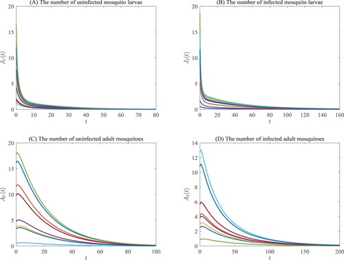
Figure 4. Assume that the parameters in system (Equation2(2) ${\begin{cases} \frac{d J_{U}}{d t} = \frac{1}{2} β A_{U} \frac{A_{U}}{A_{U} + A_{I}} - [d_{0} + d_{1} (J_{U} + J_{I})] J_{U} - α J_{U} \\ - c \frac{m J_{U}}{J_{U} + a} P := {\tilde{f}}_{1} (J_{U}, J_{I}, A_{U}, A_{I}, P), \\ \frac{d J_{I}}{d t} = \frac{1}{2} β A_{I} - [d_{0} + d_{1} (J_{U} + J_{I})] J_{I} - α J_{I} - c \frac{m J_{I}}{J_{I} + a} P := {\tilde{f}}_{2} (J_{U}, J_{I}, A_{U}, A_{I}, P), \\ \frac{d A_{U}}{d t} = α J_{U} - μ A_{U} := {\tilde{f}}_{3} (J_{U}, J_{I}, A_{U}, A_{I}, P), \\ \frac{d A_{I}}{d t} = α J_{I} - μ A_{I} := {\tilde{f}}_{4} (J_{U}, J_{I}, A_{U}, A_{I}, P), \\ \frac{d P}{d t} = \frac{m J_{U}}{J_{U} + a} P + \frac{m J_{I}}{J_{I} + a} P - δ P := {\tilde{f}}_{5} (J_{U}, J_{I}, A_{U}, A_{I}, P), \end{cases}$ (2) ) are defined the same as in Example 3.3. Then the conditions for Theorem 3.4 are satisfied, and there exists six equilibria: ${\tilde{E}}_{0}, {\tilde{E}}_{1}, {\tilde{E}}_{2}, {\tilde{E}}_{3}, {\tilde{E}}_{4}$ and ${\tilde{E}}^{*}$ . Moreover, equilibria ${\tilde{E}}_{0}, {\tilde{E}}_{1}, {\tilde{E}}_{2}$ and ${\tilde{E}}^{*}$ are unstable, equilibria ${\tilde{E}}_{3}$ and ${\tilde{E}}_{4}$ are asymptotically stable.

Figure 4. Assume that the parameters in system (Equation2(2) {dJUdt=12βAUAUAU+AI−[d0+d1(JU+JI)]JU−αJU−cmJUJU+aP:=f~1(JU,JI,AU,AI,P),dJIdt=12βAI−[d0+d1(JU+JI)]JI−αJI−cmJIJI+aP:=f~2(JU,JI,AU,AI,P),dAUdt=αJU−μAU:=f~3(JU,JI,AU,AI,P),dAIdt=αJI−μAI:=f~4(JU,JI,AU,AI,P),dPdt=mJUJU+aP+mJIJI+aP−δP:=f~5(JU,JI,AU,AI,P),(2) ) are defined the same as in Example 3.3. Then the conditions for Theorem 3.4 are satisfied, and there exists six equilibria: E~0,E~1,E~2,E~3,E~4 and E~∗. Moreover, equilibria E~0,E~1,E~2 and E~∗ are unstable, equilibria E~3 and E~4 are asymptotically stable.

4. Summary and discussion

Dengue fever results in considerable public health concern worldwide these years as the effects of traditional mosquito control methods are weakening [Citation30]. The endosymbiotic bacteria Wolbachia brings us new techniques for mosquito population control from two aspects: (i) the eggs from mating between uninfected females and infected males cannot hatch; (ii) Wolbachia-infected mosquitoes are less able to transmit dengue virus. The first mechanism inspired us to release only infected male mosquitoes for population suppression, and the second one prompted us to release both infected males and females for rapid population replacement. Since population suppression requires continuous release of infected male mosquitoes and consumes a lot of manpower and mosquito resources, we focused on the second measure in this study. Theoretically, one release based on rigorous mathematical calculation can lead to successful replacement. However, single control method is easy to be affected by uncertain factors, and also requires a relatively long waiting time. Therefore, we considered comprehensive strategies, and proposed a stage-structured five-dimensional model (Equation2(2) ${\begin{cases} \frac{d J_{U}}{d t} = \frac{1}{2} β A_{U} \frac{A_{U}}{A_{U} + A_{I}} - [d_{0} + d_{1} (J_{U} + J_{I})] J_{U} - α J_{U} \\ - c \frac{m J_{U}}{J_{U} + a} P := {\tilde{f}}_{1} (J_{U}, J_{I}, A_{U}, A_{I}, P), \\ \frac{d J_{I}}{d t} = \frac{1}{2} β A_{I} - [d_{0} + d_{1} (J_{U} + J_{I})] J_{I} - α J_{I} - c \frac{m J_{I}}{J_{I} + a} P := {\tilde{f}}_{2} (J_{U}, J_{I}, A_{U}, A_{I}, P), \\ \frac{d A_{U}}{d t} = α J_{U} - μ A_{U} := {\tilde{f}}_{3} (J_{U}, J_{I}, A_{U}, A_{I}, P), \\ \frac{d A_{I}}{d t} = α J_{I} - μ A_{I} := {\tilde{f}}_{4} (J_{U}, J_{I}, A_{U}, A_{I}, P), \\ \frac{d P}{d t} = \frac{m J_{U}}{J_{U} + a} P + \frac{m J_{I}}{J_{I} + a} P - δ P := {\tilde{f}}_{5} (J_{U}, J_{I}, A_{U}, A_{I}, P), \end{cases}$ (2) ) in this work, which includes the Wolbachia spreading dynamics in mosquitoes and the predator-prey interaction dynamics between mosquito larvae and their predators such as the arroyo chub [Citation6, Citation9, Citation11, Citation22], aimed at evaluating the impact of the introduction of the predators of mosquito larvae on Wolbachia spreading dynamics.

We started our analyses with the special system (Equation1(1) ${\begin{cases} \frac{d J_{U}}{d t} = \frac{1}{2} β A_{U} \frac{A_{U}}{A_{U} + A_{I}} - [d_{0} + d_{1} (J_{U} + J_{I})] J_{U} - α J_{U} := {\bar{f}}_{1} (J_{U}, J_{I}, A_{U}, A_{I}), \\ \frac{d J_{I}}{d t} = \frac{1}{2} β A_{I} - [d_{0} + d_{1} (J_{U} + J_{I})] J_{I} - α J_{I} := {\bar{f}}_{2} (J_{U}, J_{I}, A_{U}, A_{I}), \\ \frac{d A_{U}}{d t} = α J_{U} - μ A_{U} := {\bar{f}}_{3} (J_{U}, J_{I}, A_{U}, A_{I}), \\ \frac{d A_{I}}{d t} = α J_{I} - μ A_{I} := {\bar{f}}_{4} (J_{U}, J_{I}, A_{U}, A_{I}), \end{cases}$ (1) ) which does not include predators. This model is easier to be dealt with mathematically than system (Equation2(2) ${\begin{cases} \frac{d J_{U}}{d t} = \frac{1}{2} β A_{U} \frac{A_{U}}{A_{U} + A_{I}} - [d_{0} + d_{1} (J_{U} + J_{I})] J_{U} - α J_{U} \\ - c \frac{m J_{U}}{J_{U} + a} P := {\tilde{f}}_{1} (J_{U}, J_{I}, A_{U}, A_{I}, P), \\ \frac{d J_{I}}{d t} = \frac{1}{2} β A_{I} - [d_{0} + d_{1} (J_{U} + J_{I})] J_{I} - α J_{I} - c \frac{m J_{I}}{J_{I} + a} P := {\tilde{f}}_{2} (J_{U}, J_{I}, A_{U}, A_{I}, P), \\ \frac{d A_{U}}{d t} = α J_{U} - μ A_{U} := {\tilde{f}}_{3} (J_{U}, J_{I}, A_{U}, A_{I}, P), \\ \frac{d A_{I}}{d t} = α J_{I} - μ A_{I} := {\tilde{f}}_{4} (J_{U}, J_{I}, A_{U}, A_{I}, P), \\ \frac{d P}{d t} = \frac{m J_{U}}{J_{U} + a} P + \frac{m J_{I}}{J_{I} + a} P - δ P := {\tilde{f}}_{5} (J_{U}, J_{I}, A_{U}, A_{I}, P), \end{cases}$ (2) ), and the discussion on system (Equation1(1) ${\begin{cases} \frac{d J_{U}}{d t} = \frac{1}{2} β A_{U} \frac{A_{U}}{A_{U} + A_{I}} - [d_{0} + d_{1} (J_{U} + J_{I})] J_{U} - α J_{U} := {\bar{f}}_{1} (J_{U}, J_{I}, A_{U}, A_{I}), \\ \frac{d J_{I}}{d t} = \frac{1}{2} β A_{I} - [d_{0} + d_{1} (J_{U} + J_{I})] J_{I} - α J_{I} := {\bar{f}}_{2} (J_{U}, J_{I}, A_{U}, A_{I}), \\ \frac{d A_{U}}{d t} = α J_{U} - μ A_{U} := {\bar{f}}_{3} (J_{U}, J_{I}, A_{U}, A_{I}), \\ \frac{d A_{I}}{d t} = α J_{I} - μ A_{I} := {\bar{f}}_{4} (J_{U}, J_{I}, A_{U}, A_{I}), \end{cases}$ (1) ) can provide research ideas for the study of system (Equation2(2) ${\begin{cases} \frac{d J_{U}}{d t} = \frac{1}{2} β A_{U} \frac{A_{U}}{A_{U} + A_{I}} - [d_{0} + d_{1} (J_{U} + J_{I})] J_{U} - α J_{U} \\ - c \frac{m J_{U}}{J_{U} + a} P := {\tilde{f}}_{1} (J_{U}, J_{I}, A_{U}, A_{I}, P), \\ \frac{d J_{I}}{d t} = \frac{1}{2} β A_{I} - [d_{0} + d_{1} (J_{U} + J_{I})] J_{I} - α J_{I} - c \frac{m J_{I}}{J_{I} + a} P := {\tilde{f}}_{2} (J_{U}, J_{I}, A_{U}, A_{I}, P), \\ \frac{d A_{U}}{d t} = α J_{U} - μ A_{U} := {\tilde{f}}_{3} (J_{U}, J_{I}, A_{U}, A_{I}, P), \\ \frac{d A_{I}}{d t} = α J_{I} - μ A_{I} := {\tilde{f}}_{4} (J_{U}, J_{I}, A_{U}, A_{I}, P), \\ \frac{d P}{d t} = \frac{m J_{U}}{J_{U} + a} P + \frac{m J_{I}}{J_{I} + a} P - δ P := {\tilde{f}}_{5} (J_{U}, J_{I}, A_{U}, A_{I}, P), \end{cases}$ (2) ). We first proved that system (Equation1(1) ${\begin{cases} \frac{d J_{U}}{d t} = \frac{1}{2} β A_{U} \frac{A_{U}}{A_{U} + A_{I}} - [d_{0} + d_{1} (J_{U} + J_{I})] J_{U} - α J_{U} := {\bar{f}}_{1} (J_{U}, J_{I}, A_{U}, A_{I}), \\ \frac{d J_{I}}{d t} = \frac{1}{2} β A_{I} - [d_{0} + d_{1} (J_{U} + J_{I})] J_{I} - α J_{I} := {\bar{f}}_{2} (J_{U}, J_{I}, A_{U}, A_{I}), \\ \frac{d A_{U}}{d t} = α J_{U} - μ A_{U} := {\bar{f}}_{3} (J_{U}, J_{I}, A_{U}, A_{I}), \\ \frac{d A_{I}}{d t} = α J_{I} - μ A_{I} := {\bar{f}}_{4} (J_{U}, J_{I}, A_{U}, A_{I}), \end{cases}$ (1) ) has no positive equilibria. Then under two cases $0 < β < β^{*}$ and $β > β^{*}$ , we derived the numbers of equilibria and their corresponding stabilities. More precisely, for the case with $0 < β < β^{*}$ , we found that system (Equation1(1) ${\begin{cases} \frac{d J_{U}}{d t} = \frac{1}{2} β A_{U} \frac{A_{U}}{A_{U} + A_{I}} - [d_{0} + d_{1} (J_{U} + J_{I})] J_{U} - α J_{U} := {\bar{f}}_{1} (J_{U}, J_{I}, A_{U}, A_{I}), \\ \frac{d J_{I}}{d t} = \frac{1}{2} β A_{I} - [d_{0} + d_{1} (J_{U} + J_{I})] J_{I} - α J_{I} := {\bar{f}}_{2} (J_{U}, J_{I}, A_{U}, A_{I}), \\ \frac{d A_{U}}{d t} = α J_{U} - μ A_{U} := {\bar{f}}_{3} (J_{U}, J_{I}, A_{U}, A_{I}), \\ \frac{d A_{I}}{d t} = α J_{I} - μ A_{I} := {\bar{f}}_{4} (J_{U}, J_{I}, A_{U}, A_{I}), \end{cases}$ (1) ) admits ${\bar{E}}_{0}$ as its unique equilibrium, and it is globally attractive. While for the case with $β > β^{*}$ , we observed that the system has exactly three equilibria, that is, ${\bar{E}}_{0}, {\bar{E}}_{1}$ and ${\bar{E}}_{2}$ . Moreover, the equilibria ${\bar{E}}_{0}$ and ${\bar{E}}_{2}$ are unstable, while the equilibrium ${\bar{E}}_{1}$ is asymptotically stable.

Subsequently, we explored the dynamics of the five dimensional system (Equation2(2) ${\begin{cases} \frac{d J_{U}}{d t} = \frac{1}{2} β A_{U} \frac{A_{U}}{A_{U} + A_{I}} - [d_{0} + d_{1} (J_{U} + J_{I})] J_{U} - α J_{U} \\ - c \frac{m J_{U}}{J_{U} + a} P := {\tilde{f}}_{1} (J_{U}, J_{I}, A_{U}, A_{I}, P), \\ \frac{d J_{I}}{d t} = \frac{1}{2} β A_{I} - [d_{0} + d_{1} (J_{U} + J_{I})] J_{I} - α J_{I} - c \frac{m J_{I}}{J_{I} + a} P := {\tilde{f}}_{2} (J_{U}, J_{I}, A_{U}, A_{I}, P), \\ \frac{d A_{U}}{d t} = α J_{U} - μ A_{U} := {\tilde{f}}_{3} (J_{U}, J_{I}, A_{U}, A_{I}, P), \\ \frac{d A_{I}}{d t} = α J_{I} - μ A_{I} := {\tilde{f}}_{4} (J_{U}, J_{I}, A_{U}, A_{I}, P), \\ \frac{d P}{d t} = \frac{m J_{U}}{J_{U} + a} P + \frac{m J_{I}}{J_{I} + a} P - δ P := {\tilde{f}}_{5} (J_{U}, J_{I}, A_{U}, A_{I}, P), \end{cases}$ (2) ) under the assumptions $(A 1)$ - $(A 3)$ , and observed that (Equation2(2) ${\begin{cases} \frac{d J_{U}}{d t} = \frac{1}{2} β A_{U} \frac{A_{U}}{A_{U} + A_{I}} - [d_{0} + d_{1} (J_{U} + J_{I})] J_{U} - α J_{U} \\ - c \frac{m J_{U}}{J_{U} + a} P := {\tilde{f}}_{1} (J_{U}, J_{I}, A_{U}, A_{I}, P), \\ \frac{d J_{I}}{d t} = \frac{1}{2} β A_{I} - [d_{0} + d_{1} (J_{U} + J_{I})] J_{I} - α J_{I} - c \frac{m J_{I}}{J_{I} + a} P := {\tilde{f}}_{2} (J_{U}, J_{I}, A_{U}, A_{I}, P), \\ \frac{d A_{U}}{d t} = α J_{U} - μ A_{U} := {\tilde{f}}_{3} (J_{U}, J_{I}, A_{U}, A_{I}, P), \\ \frac{d A_{I}}{d t} = α J_{I} - μ A_{I} := {\tilde{f}}_{4} (J_{U}, J_{I}, A_{U}, A_{I}, P), \\ \frac{d P}{d t} = \frac{m J_{U}}{J_{U} + a} P + \frac{m J_{I}}{J_{I} + a} P - δ P := {\tilde{f}}_{5} (J_{U}, J_{I}, A_{U}, A_{I}, P), \end{cases}$ (2) ) admits five boundary equilibria, that is, the origin ${\tilde{E}}_{0}$ , and four boundary equilibria ${\tilde{E}}_{1}, {\tilde{E}}_{2}, {\tilde{E}}_{3}, {\tilde{E}}_{4}$ . Moreover, to explore the number of positive equilibria of system (Equation2(2) ${\begin{cases} \frac{d J_{U}}{d t} = \frac{1}{2} β A_{U} \frac{A_{U}}{A_{U} + A_{I}} - [d_{0} + d_{1} (J_{U} + J_{I})] J_{U} - α J_{U} \\ - c \frac{m J_{U}}{J_{U} + a} P := {\tilde{f}}_{1} (J_{U}, J_{I}, A_{U}, A_{I}, P), \\ \frac{d J_{I}}{d t} = \frac{1}{2} β A_{I} - [d_{0} + d_{1} (J_{U} + J_{I})] J_{I} - α J_{I} - c \frac{m J_{I}}{J_{I} + a} P := {\tilde{f}}_{2} (J_{U}, J_{I}, A_{U}, A_{I}, P), \\ \frac{d A_{U}}{d t} = α J_{U} - μ A_{U} := {\tilde{f}}_{3} (J_{U}, J_{I}, A_{U}, A_{I}, P), \\ \frac{d A_{I}}{d t} = α J_{I} - μ A_{I} := {\tilde{f}}_{4} (J_{U}, J_{I}, A_{U}, A_{I}, P), \\ \frac{d P}{d t} = \frac{m J_{U}}{J_{U} + a} P + \frac{m J_{I}}{J_{I} + a} P - δ P := {\tilde{f}}_{5} (J_{U}, J_{I}, A_{U}, A_{I}, P), \end{cases}$ (2) ), we first noticed that a potential positive equilibrium of (Equation2(2) ${\begin{cases} \frac{d J_{U}}{d t} = \frac{1}{2} β A_{U} \frac{A_{U}}{A_{U} + A_{I}} - [d_{0} + d_{1} (J_{U} + J_{I})] J_{U} - α J_{U} \\ - c \frac{m J_{U}}{J_{U} + a} P := {\tilde{f}}_{1} (J_{U}, J_{I}, A_{U}, A_{I}, P), \\ \frac{d J_{I}}{d t} = \frac{1}{2} β A_{I} - [d_{0} + d_{1} (J_{U} + J_{I})] J_{I} - α J_{I} - c \frac{m J_{I}}{J_{I} + a} P := {\tilde{f}}_{2} (J_{U}, J_{I}, A_{U}, A_{I}, P), \\ \frac{d A_{U}}{d t} = α J_{U} - μ A_{U} := {\tilde{f}}_{3} (J_{U}, J_{I}, A_{U}, A_{I}, P), \\ \frac{d A_{I}}{d t} = α J_{I} - μ A_{I} := {\tilde{f}}_{4} (J_{U}, J_{I}, A_{U}, A_{I}, P), \\ \frac{d P}{d t} = \frac{m J_{U}}{J_{U} + a} P + \frac{m J_{I}}{J_{I} + a} P - δ P := {\tilde{f}}_{5} (J_{U}, J_{I}, A_{U}, A_{I}, P), \end{cases}$ (2) ) must satisfy (Equation17(17) ${\begin{cases} \frac{1}{2} β {\tilde{A}}_{U}^{*} \frac{{\tilde{A}}_{U}^{*}}{{\tilde{A}}_{U}^{*} + {\tilde{A}}_{I}^{*}} - (d_{0} + d_{1} ({\tilde{J}}_{U}^{*} + {\tilde{J}}_{I}^{*})) {\tilde{J}}_{U}^{*} - α {\tilde{J}}_{U}^{*} - c \frac{m {\tilde{J}}_{U}^{*}}{{\tilde{J}}_{U}^{*} + a} {\tilde{P}}^{*} = 0, \\ \frac{1}{2} β {\tilde{A}}_{I}^{*} - (d_{0} + d_{1} ({\tilde{J}}_{U}^{*} + {\tilde{J}}_{I}^{*})) {\tilde{J}}_{I}^{*} - α {\tilde{J}}_{I}^{*} - c \frac{m {\tilde{J}}_{I}^{*}}{{\tilde{J}}_{I}^{*} + a} {\tilde{P}}^{*} = 0, \\ α {\tilde{J}}_{U}^{*} - μ {\tilde{A}}_{U}^{*} = 0, \\ α {\tilde{J}}_{I}^{*} - μ {\tilde{A}}_{I}^{*} = 0, \\ \frac{m {\tilde{J}}_{U}^{*}}{{\tilde{J}}_{U}^{*} + a} {\tilde{P}}^{*} + \frac{m {\tilde{J}}_{I}^{*}}{{\tilde{J}}_{I}^{*} + a} {\tilde{P}}^{*} - δ {\tilde{P}}^{*} = 0, \end{cases}$ (17) ), and then we equivalently transformed the problem of the number of positive equilibria of (Equation2(2) ${\begin{cases} \frac{d J_{U}}{d t} = \frac{1}{2} β A_{U} \frac{A_{U}}{A_{U} + A_{I}} - [d_{0} + d_{1} (J_{U} + J_{I})] J_{U} - α J_{U} \\ - c \frac{m J_{U}}{J_{U} + a} P := {\tilde{f}}_{1} (J_{U}, J_{I}, A_{U}, A_{I}, P), \\ \frac{d J_{I}}{d t} = \frac{1}{2} β A_{I} - [d_{0} + d_{1} (J_{U} + J_{I})] J_{I} - α J_{I} - c \frac{m J_{I}}{J_{I} + a} P := {\tilde{f}}_{2} (J_{U}, J_{I}, A_{U}, A_{I}, P), \\ \frac{d A_{U}}{d t} = α J_{U} - μ A_{U} := {\tilde{f}}_{3} (J_{U}, J_{I}, A_{U}, A_{I}, P), \\ \frac{d A_{I}}{d t} = α J_{I} - μ A_{I} := {\tilde{f}}_{4} (J_{U}, J_{I}, A_{U}, A_{I}, P), \\ \frac{d P}{d t} = \frac{m J_{U}}{J_{U} + a} P + \frac{m J_{I}}{J_{I} + a} P - δ P := {\tilde{f}}_{5} (J_{U}, J_{I}, A_{U}, A_{I}, P), \end{cases}$ (2) ) to the problem of the number of positive real roots of (Equation18(18) $F (x) = R_{6} x^{6} + R_{5} x^{5} + R_{4} x^{4} + R_{3} x^{3} + R_{2} x^{2} + R_{1} x + R_{0},$ (18) ) in a given range. By applying the Descartes's rule of signs, we finally proved that system (Equation2(2) ${\begin{cases} \frac{d J_{U}}{d t} = \frac{1}{2} β A_{U} \frac{A_{U}}{A_{U} + A_{I}} - [d_{0} + d_{1} (J_{U} + J_{I})] J_{U} - α J_{U} \\ - c \frac{m J_{U}}{J_{U} + a} P := {\tilde{f}}_{1} (J_{U}, J_{I}, A_{U}, A_{I}, P), \\ \frac{d J_{I}}{d t} = \frac{1}{2} β A_{I} - [d_{0} + d_{1} (J_{U} + J_{I})] J_{I} - α J_{I} - c \frac{m J_{I}}{J_{I} + a} P := {\tilde{f}}_{2} (J_{U}, J_{I}, A_{U}, A_{I}, P), \\ \frac{d A_{U}}{d t} = α J_{U} - μ A_{U} := {\tilde{f}}_{3} (J_{U}, J_{I}, A_{U}, A_{I}, P), \\ \frac{d A_{I}}{d t} = α J_{I} - μ A_{I} := {\tilde{f}}_{4} (J_{U}, J_{I}, A_{U}, A_{I}, P), \\ \frac{d P}{d t} = \frac{m J_{U}}{J_{U} + a} P + \frac{m J_{I}}{J_{I} + a} P - δ P := {\tilde{f}}_{5} (J_{U}, J_{I}, A_{U}, A_{I}, P), \end{cases}$ (2) ) has a unique positive equilibrium ${\tilde{E}}^{*}$ . For the stabilities, we first found that the equilibria ${\tilde{E}}_{0}, {\tilde{E}}_{1}$ and ${\tilde{E}}_{2}$ are unstable, and then by employing the Routh-Hurwitz criterion, we showed that the equilibria ${\tilde{E}}_{3}$ and ${\tilde{E}}_{4}$ are asymptotically stable, while the stability of ${\tilde{E}}^{*}$ is not clear in the present time. We mention here that Figure just depicts the asymptotic stability of ${\tilde{E}}_{3}$ . For the asymptotic stability of ${\tilde{E}}_{4}$ , a similar figure as Figure can be obtained.

Biologically, if we consider the reduced three-dimensional system composed of $J_{U}, J_{I}$ and P, the equilibria ${\tilde{E}}_{3}, {\tilde{E}}_{4}$ and ${\tilde{E}}^{*}$ describe three types of coexistence phenomena: the coexistence of infected mosquito larvae and their predators, the coexistence of uninfected mosquito larvae and their predators and the coexistence of the three of them, respectively. Compared the number of equilibria of (Equation2(2) ${\begin{cases} \frac{d J_{U}}{d t} = \frac{1}{2} β A_{U} \frac{A_{U}}{A_{U} + A_{I}} - [d_{0} + d_{1} (J_{U} + J_{I})] J_{U} - α J_{U} \\ - c \frac{m J_{U}}{J_{U} + a} P := {\tilde{f}}_{1} (J_{U}, J_{I}, A_{U}, A_{I}, P), \\ \frac{d J_{I}}{d t} = \frac{1}{2} β A_{I} - [d_{0} + d_{1} (J_{U} + J_{I})] J_{I} - α J_{I} - c \frac{m J_{I}}{J_{I} + a} P := {\tilde{f}}_{2} (J_{U}, J_{I}, A_{U}, A_{I}, P), \\ \frac{d A_{U}}{d t} = α J_{U} - μ A_{U} := {\tilde{f}}_{3} (J_{U}, J_{I}, A_{U}, A_{I}, P), \\ \frac{d A_{I}}{d t} = α J_{I} - μ A_{I} := {\tilde{f}}_{4} (J_{U}, J_{I}, A_{U}, A_{I}, P), \\ \frac{d P}{d t} = \frac{m J_{U}}{J_{U} + a} P + \frac{m J_{I}}{J_{I} + a} P - δ P := {\tilde{f}}_{5} (J_{U}, J_{I}, A_{U}, A_{I}, P), \end{cases}$ (2) ) with that of (Equation1(1) ${\begin{cases} \frac{d J_{U}}{d t} = \frac{1}{2} β A_{U} \frac{A_{U}}{A_{U} + A_{I}} - [d_{0} + d_{1} (J_{U} + J_{I})] J_{U} - α J_{U} := {\bar{f}}_{1} (J_{U}, J_{I}, A_{U}, A_{I}), \\ \frac{d J_{I}}{d t} = \frac{1}{2} β A_{I} - [d_{0} + d_{1} (J_{U} + J_{I})] J_{I} - α J_{I} := {\bar{f}}_{2} (J_{U}, J_{I}, A_{U}, A_{I}), \\ \frac{d A_{U}}{d t} = α J_{U} - μ A_{U} := {\bar{f}}_{3} (J_{U}, J_{I}, A_{U}, A_{I}), \\ \frac{d A_{I}}{d t} = α J_{I} - μ A_{I} := {\bar{f}}_{4} (J_{U}, J_{I}, A_{U}, A_{I}), \end{cases}$ (1) ), it is expected that the introduction of the predators will augment the number of coexistence equilibria. For system (Equation1(1) ${\begin{cases} \frac{d J_{U}}{d t} = \frac{1}{2} β A_{U} \frac{A_{U}}{A_{U} + A_{I}} - [d_{0} + d_{1} (J_{U} + J_{I})] J_{U} - α J_{U} := {\bar{f}}_{1} (J_{U}, J_{I}, A_{U}, A_{I}), \\ \frac{d J_{I}}{d t} = \frac{1}{2} β A_{I} - [d_{0} + d_{1} (J_{U} + J_{I})] J_{I} - α J_{I} := {\bar{f}}_{2} (J_{U}, J_{I}, A_{U}, A_{I}), \\ \frac{d A_{U}}{d t} = α J_{U} - μ A_{U} := {\bar{f}}_{3} (J_{U}, J_{I}, A_{U}, A_{I}), \\ \frac{d A_{I}}{d t} = α J_{I} - μ A_{I} := {\bar{f}}_{4} (J_{U}, J_{I}, A_{U}, A_{I}), \end{cases}$ (1) ), ${\bar{E}}_{1}$ is asymptotically stable and ${\bar{E}}_{2}$ is unstable, which indicates that population replacement is easy to achieve. However, for system (Equation2(2) ${\begin{cases} \frac{d J_{U}}{d t} = \frac{1}{2} β A_{U} \frac{A_{U}}{A_{U} + A_{I}} - [d_{0} + d_{1} (J_{U} + J_{I})] J_{U} - α J_{U} \\ - c \frac{m J_{U}}{J_{U} + a} P := {\tilde{f}}_{1} (J_{U}, J_{I}, A_{U}, A_{I}, P), \\ \frac{d J_{I}}{d t} = \frac{1}{2} β A_{I} - [d_{0} + d_{1} (J_{U} + J_{I})] J_{I} - α J_{I} - c \frac{m J_{I}}{J_{I} + a} P := {\tilde{f}}_{2} (J_{U}, J_{I}, A_{U}, A_{I}, P), \\ \frac{d A_{U}}{d t} = α J_{U} - μ A_{U} := {\tilde{f}}_{3} (J_{U}, J_{I}, A_{U}, A_{I}, P), \\ \frac{d A_{I}}{d t} = α J_{I} - μ A_{I} := {\tilde{f}}_{4} (J_{U}, J_{I}, A_{U}, A_{I}, P), \\ \frac{d P}{d t} = \frac{m J_{U}}{J_{U} + a} P + \frac{m J_{I}}{J_{I} + a} P - δ P := {\tilde{f}}_{5} (J_{U}, J_{I}, A_{U}, A_{I}, P), \end{cases}$ (2) ), both ${\tilde{E}}_{3}$ and ${\tilde{E}}_{4}$ are asymptotically stable, implying that Wolbachia-infected mosquitoes no longer have huge advantage in competition with uninfected mosquitoes. We conclude that the introduction of the predators of mosquito larvae may hinder the spread of Wolbachia in mosquitoes. The reason for the difference may be the introduced predators prey on uninfected and infected mosquito larvae equally, which declines the infection frequency of wild mosquito population and not conducive to the spread of Wolbachia in mosquitoes. 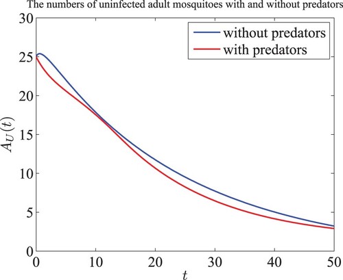Although the introduction of predators transforms ${\tilde{E}}_{4}$ from unstable equilibrium to locally stable equilibrium, it quickly reduce the number of uninfected adult mosquitoes (see Figure ) and then reduce the risk of mosquito-borne diseases transmission. The combination of the two strategies can more effectively control mosquito populations, we will carefully study this effective combination in our future work.

Figure 5. We choose the parameters in Figures C and C and set $A_{U} (0) = 25$ . Then obtain the numbers of uninfected adult mosquitoes with and without predators.

Figure 5. We choose the parameters in Figures 2C and 4C and set AU(0)=25. Then obtain the numbers of uninfected adult mosquitoes with and without predators.

Acknowledgments

We thank the editors and two anonymous reviewers for their careful reading and valuable comments and suggestions.

Disclosure statement

No potential conflict of interest was reported by the author(s).

Data availability statements

Data sharing is not applicable to this article as no new data were created or analysed in this study.

Additional information

Funding

This work was supported by National Natural Science Foundation of China [12171112], Guangdong Basic and Applied Basic Research Foundation [2023A1515011570] and Natural Science Foundation of Henan Province [232300420127].

References

S. Ai, J. Li, J. Yu, and B. Zheng, Stage-structured models for interactive wild and periodically and impulsively released sterile mosquitoes, Discrete Contin. Dyn. Syst. Ser. B. 27(6) (2022), pp. 3039–3052.
Web of Science ®Google Scholar
G. Bian, Y. Xu, P. Lu, Y. Xie, and Z. Xi, The endosymbiotic bacterium wolbachia induces resistance to dengue virus in aedes aegypti, PLoS. Pathog. 6(4) (2010), pp. e1000833.
PubMed Web of Science ®Google Scholar
F. Brauer and C. Castillo-Chavez, Mathematical Models in Population Biology and Epidemiology, Springer New York, New York, NY, 2012.
Google Scholar
L. Cai, S. Ai, and J. Li, Dynamics of mosquitoes populations with different strategies for releasing sterile mosquitoes, SIAM. J. Appl. Math. 74(6) (2014), pp. 1786–1809.
Web of Science ®Google Scholar
C. Castillo-Chavez and B.J. Song, Dynamical models of tuberculosis and their applications, Math. Biosci. Eng. 1(2) (2004), pp. 361–404.
PubMed Web of Science ®Google Scholar
P. Dambach, The use of aquatic predators for larval control of mosquito disease vectors: opportunities and limitations, Biol. Control. 150 (2020), pp. 104357.
Web of Science ®Google Scholar
Dengue, Technical report, World Mosquito Program, 2022.
Google Scholar
H.I. Freedman, Deterministic Mathematical Models in Population Ecology, Marcel Dekker, New York, 1980.
Google Scholar
M. Ghosh, A. Lashari, and X.-Z. Li, Biological control of malaria: A mathematical model, Appl. Math. Comput. 219(15) (2013), pp. 7923–7939.
Web of Science ®Google Scholar
J.-T. Gong, T.-P. Li, M.-K. Wang, and X.-Y. Hong, Wolbachia-based strategies for control of agricultural pests, Curr. Opin. Insect. Sci. 57 (2023). doi:10.1016/j.cois.2023.101039
PubMed Web of Science ®Google Scholar
L.F. Griffin and J.M. Knight, A review of the role of fish as biological control agents of disease vector mosquitoes in mangrove forests: reducing human health risks while reducing environmental risk, Wetl. Ecol. Manag. 20(3) (2012), pp. 243–252.
Web of Science ®Google Scholar
S.B. Hsu, T.W. Hwang, and Y. Kuang, Global analysis of the michaelis-menten-type ratio-dependent predator-prey system, J. Math. Biol. 42(6) (2001), pp. 489–506.
PubMed Web of Science ®Google Scholar
S.B. Hsu, T.W. Hwang, and Y. Kuang, A ratio-dependent food chain model and its applications to biological control, Math. Biosci. 181(1) (2003), pp. 55–83.
PubMed Web of Science ®Google Scholar
L. Hu, M. Tang, Z. Wu, Z. Xi, and J. Yu, The threshold infection level for wolbachia invasion in random environments, J. Differ. Equ. 266(7) (2019), pp. 4377–4393.
Web of Science ®Google Scholar
M. Huang, S. Liu, and X. Song, Modeling of periodic compensation policy for sterile mosquitoes incorporating sexual lifespan, Math. Methods. Appl. Sci. 46(5) (2023), pp. 5725–5741.
Web of Science ®Google Scholar
M. Huang, X. Song, and J. Li, Modelling and analysis of impulsive releases of sterile mosquitoes, J. Biol. Dyn. 11(1) (2017), pp. 147–171.
PubMed Web of Science ®Google Scholar
Y. Hui, G. Lin, J. Yu, and J. Li, A delayed differential equation model for mosquito population suppression with sterile mosquitoes, Discrete Contin. Dyn. Syst. Ser. B. 25(12) (2020), pp. 4659–4676.
Web of Science ®Google Scholar
M. Kot, Elements of Mathematical Ecology, Cambridge University Press, Cambridge, UK, 2001.
Google Scholar
Y. Kuang and E. Beretta, Global qualitative analysis of a ratio-dependent predator-prey system, J. Math. Biol. 36 (1998), pp. 389–406.
Web of Science ®Google Scholar
Y. Kuang and K. Wang, Coexistence and extinction in a data-based ratio-dependent model of an insect community, Math. Biosci. Eng. 17(4) (2020), pp. 3274–3293.
PubMed Web of Science ®Google Scholar
J. Li and S. Ai, Impulsive releases of sterile mosquitoes and interactive dynamics with time delay, J. Biol. Dyn. 14(1) (2020), pp. 313–331.
PubMed Web of Science ®Google Scholar
Y. Lou and X.-Q. Zhao, Modelling malaria control by introduction of larvivorous fish, Bull. Math. Biol. 73(10) (2011), pp. 2384–2407.
PubMed Web of Science ®Google Scholar
R.M. May, Stability and Complexity in Model Ecosystems (Princeton Landmarks in Biology), Princeton University, Princeton, 2001.
Google Scholar
C.J. McMeniman, R.V. Lane, B.N. Cass, A.W.C. Fong, M. Sidhu, Y.-F. Wang, and S.L. O'Neill, Stable introduction of a life-shortening wolbachia infection into the mosquito aedes aegypti, Science323(5910) (2009), pp. 141–144.
PubMed Web of Science ®Google Scholar
H. MuGen, T. MoXun, and Y. JianShe, Wolbachia infection dynamics by reaction-diffusion equations, Sci. China-Math. 58(1) (2015), pp. 77–96.
Web of Science ®Google Scholar
H. Quiroz-Martinez and A. Rodriguez-Castro, Aquatic insects as predators of mosquito larvae, J. Am. Mosq. Control. Assoc. 23(sp2) (2007), pp. 110–117.
PubMedGoogle Scholar
Y. Shi and B. Zheng, Modeling wolbachia infection frequency in mosquito populations via a continuous periodic switching model, Adv. Nonlinear Anal. 12(1) (2023). doi:10.1515/anona-2022-0297
Web of Science ®Google Scholar
H.L. Smith, (mathematical surveys and monographs). Monotone Dynamical Systems: An Introduction to the Theory of Competitive and Cooperative Systems. 1995.
Google Scholar
H.L. Smith and P. Waltman, The Theory of the Chemostat: Dynamics of Microbial Competition, Cambridge Studies in Mathematical Biology, Cambridge University Press, Cambridge, UK, 1995.
Google Scholar
M.A. Tolle, Mosquito-borne diseases, Curr. Probl. Pediatr. Adolesc. Health. Care. 39(4) (2009), pp. 97–140.
PubMedGoogle Scholar
M. Turelli and A.A. Hoffmann, Rapid spread of an inherited incompatibility factor in california drosophila, Nature 353(6343) (1991), pp. 440–442.
PubMed Web of Science ®Google Scholar
A.R. Van Dam and W.E. Walton, Comparison of mosquito control provided by the arroyo chub (gilaorcutti) and the mosquitofish (gambusia affinis), J. Am. Mosq. Control. Assoc. 23(4) (2007), pp. 430–441.
PubMed Web of Science ®Google Scholar
T. Walker, P.H. Johnson, L.A. Moreira, I. Iturbe-Ormaetxe, F.D. Frentiu, C.J. McMeniman, Y.S.Leong, Y. Dong, J. Axford, P. Kriesner, A.L. Lloyd, S.A. Ritchie, S.L. O'Neill, and A.A. Hoffmann, The wmel wolbachia strain blocks dengue and invades caged aedes aegypti populations, Nature 476(7361) (2011), pp. 450–453.
PubMed Web of Science ®Google Scholar
Z.Y. Xi, C.C.H. Khoo, and S.L. Dobson, Wolbachia establishment and invasion in an aedes aegypti laboratory population, Science 310(5746) (2005), pp. 326–328.
PubMed Web of Science ®Google Scholar
R. Yan, B. Zheng, and J. Yu, Existence and stability of periodic solutions for a mosquito suppression model with incomplete cytoplasmic incompatibility, Discrete Contin. Dyn. Syst. Ser. B. 28(5) (2023), pp. 3172–3192.
Web of Science ®Google Scholar
J. Yu, Modeling mosquito population suppression based on delay differential equations, SIAM. J. Appl. Math. 78(6) (2018), pp. 3168–3187.
Web of Science ®Google Scholar
J. Yu, Existence and stability of a unique and exact two periodic orbits for an interactive wild and sterile mosquito model, J. Differ. Equ. 269(12) (2020), pp. 10395–10415.
Web of Science ®Google Scholar
J. Yu and J. Li, Dynamics of interactive wild and sterile mosquitoes with time delay, J. Biol. Dyn.13(1) (2019), pp. 606–620.
PubMed Web of Science ®Google Scholar
J. Yu and J. Li, Global asymptotic stability in an interactive wild and sterile mosquito model, J. Differ. Equ. 269(7) (2020), pp. 6193–6215.
Web of Science ®Google Scholar
D. Zhang, Y. Sun, H. Yamada, Y. Wu, G. Wang, Q. Feng, D. Paerhande, H. Maiga, J. Bouyer, J.Qian, Z. Wu, and X. Zheng, Effects of radiation on the fitness, sterility and arbovirus susceptibility of a wolbachia-free aedes albopictus strain for use in the sterile insect technique, Pest. Manag. Sci. 2023 (2023). doi:10.1002/ps.7615
Google Scholar
X. Zhang, S. Tang, and R.A. Cheke, Models to assess how best to replace dengue virus vectors with wolbachia-infected mosquito populations, Math. Biosci. 269 (2015), pp. 164–177.
PubMed Web of Science ®Google Scholar
B. Zheng, M. Tang, J. Yu, and J. Qiu, Wolbachia spreading dynamics in mosquitoes with imperfect maternal transmission, J. Math. Biol. 76(1-2) (2018), pp. 235–263.
PubMed Web of Science ®Google Scholar
B. Zheng and J. Yu, At most two periodic solutions for a switching mosquito population suppression model, J. Dyn. Differ. Equ. 2022 (2022). doi:10.1007/s10884-021-10125-y
Google Scholar
Z. Zhu, X. Feng, and L. Hu, Global dynamics of a mosquito population suppression model under a periodic release strategy, J. Appl. Anal.Comput. 13(4) (2023), pp. 2297–2314.
Google Scholar
Z. Zhu, B. Zheng, Y. Shi, R. Yan, and J. Yu, Stability and periodicity in a mosquito population suppression model composed of two sub-models, Nonlinear. Dyn. 107(1) (2022), pp. 1383–1395.
Web of Science ®Google Scholar
W.F. Zuharah and P.J. Lester, The influence of aquatic predators on mosquito abundance in animal drinking troughs in new zealand, J. Vector. Ecol. 35(2) (2010), pp. 347–353.
PubMed Web of Science ®Google Scholar

The impact of predators of mosquito larvae on Wolbachia spreading dynamics

Abstract

1. Introduction

Table 1. Model parameters and their interpretations.

2. Uniqueness, positivity and boundedness

3. Main results

3.1. Dynamics of the system without predators

3.1.1. Structure of equilibria of system (1)

3.1.2. Stabilities of equilibria of system (1)

[Citation5]

3.2. Dynamics of the system with predators

3.2.1. Structure of equilibria of system (2)

3.2.2. Stabilities of equilibria of system (2)

4. Summary and discussion

Acknowledgments

Disclosure statement

Data availability statements

References

Information for

Open access

Opportunities

Help and information

The impact of predators of mosquito larvae on Wolbachia spreading dynamics

Abstract

1. Introduction

Table 1. Model parameters and their interpretations.

2. Uniqueness, positivity and boundedness

3. Main results

3.1. Dynamics of the system without predators

3.1.1. Structure of equilibria of system (1)

3.1.2. Stabilities of equilibria of system (1)

[Citation5]

3.2. Dynamics of the system with predators

3.2.1. Structure of equilibria of system (2)

3.2.2. Stabilities of equilibria of system (2)

4. Summary and discussion

Acknowledgments

Disclosure statement

Data availability statements

Additional information

Funding

References

Related research

To cite this article:

Download citation

Your download is now in progress and you may close this window

Login or register to access this feature

Information for

Open access

Opportunities

Help and information

Keep up to date