Global dynamics of discrete mathematical models of tuberculosis

Abstract

In this paper, we develop discrete models of Tuberculosis (TB). This includes SEI endogenous and exogenous models without treatment. These models are then extended to a SEIT model with treatment. We develop two types of net reproduction numbers, one is the traditional ${\mathcal{R}}_0$ which is based on the disease-free equilibrium, and a new net reproduction number ${\mathcal{R}}_0\left({\mathcal{E}}^{\ast }\right)$ based on the endemic equilibrium. It is shown that the disease-free equilibrium is globally asymptotically stable if ${\mathcal{R}}_0\le 1$ and unstable if ${\mathcal{R}}_0>1$. Moreover, the endemic equilibrium is locally asymptotically stable if ${\mathcal{R}}_0\left({\mathcal{E}}^{\ast }\right)<1<{\mathcal{R}}_0$.

KEYWORDS:

• Tuberculosis
• treatment
• disease-free
• endemic
• endogenous
• exogenous
• local stability
• global stability
• SEI models
• SEIT models
• disease control
• treatment
• epidemiology
• public health
• TB elimination

MATHEMATICS SUBJECT CLASSIFICATIONS:

• 92-10
• 39A30

1. Introduction

Tuberculosis (TB) remains a formidable global health challenge, affecting millions of individuals across the globe. The disease's complex transmission dynamics and its ability to persist in various populations have spurred the need for a comprehensive understanding of TB and effective control measures. Mathematical modelling has emerged as a powerful tool to gain insights into the intricate dynamics of TB transmission and evaluate potential interventions. The foundations of mathematical epidemiology based on compartmental models are due to Sir Ronald Ross, who gave the first mathematical model of malaria transmission in 1911 [1].

In this research paper, we embark on a thorough exploration of the global dynamics of discrete mathematical models of Tuberculosis.

We investigate both SEI (Susceptible-Exposed-Infectious) and SEIT (Susceptible-Exposed-Infectious-Treated) models with endogenous and exogenous components to elucidate the complexities of TB transmission and its implications for global public health.

Once someone is exposed, TB bacteria can live in the human or animal body for years if not decades without any symptoms, called latent TB infection. In fact, many people who have latent TB never develop the infectious disease, but they still test positive, though not infectious, meaning they cannot spread TB bacteria to others. To elaborate the progression from exposed to infected, TB bacteria enter the lungs, then as blood circulates, transporting them–of course, because the lungs oxygenate blood and/or cells–to other parts of the body, they infect a kidney, the spine or brain, which are generally not transmissible. TB bacteria turns into an active infection if the immune system cannot stem the growth rate. Common symptoms of tuberculosis are chest pain, weight loss, fever, a persistent cough that may contain blood, etc.

Nevertheless, active TB infection can be treated by prolonged use of antibiotics. In 1943, Selman Waksman, Elizabeth Bugie, and Albert Schatz developed streptomycin, the first antibiotic, whereas rest and sunlight were prescribed in sanatoriums to alleviate TB. It was later abandoned because it induces permanent hearing loss, tinnitus, dizziness, and vertigo [2].

Now, four drugs are used in therapy: isoniazid (1951), pyrazinamide (1952), ethambutol (1961), and rifampin (1966) [3]. They remain the most common treatment for TB (CDC).

With that said, another difficulty is that many strains of TB are drug-resistant. We conclude the SEIT model is sufficient to describe the transmission pattern of tuberculosis. However, the reality is that while models assume we have access to complete data on TB cases, every active infection is not reported. Moreover, since latent TB carriers exhibit no symptoms, their exact number is far more difficult to estimate, and treatment often goes half-done because of its length or duration [4]. Above all, tuberculosis is a disease of poverty, which is not difficult to predict given that nations with higher living standards report fewer cases of TB.

For decades it has been assumed that postprimary tuberculosis is usually caused by the reactivation of endogenous infection rather than by a new, exogenous infection. However, Exogenous reinfection appears to be a major cause of postprimary tuberculosis after a previous cure in an area with a high incidence of this disease. This finding emphasizes the importance of achieving cures and of preventing anyone with infectious tuberculosis from exposing others to the disease.

TB has plagued humanity for millennia, shaping historical narratives and leaving a profound impact on societies worldwide. Known as ”consumption” and ”phthisis” in different periods, TB was associated with suffering and mortality, and its impact can be traced through historical artifacts, art, and literature. The 19th century witnessed a devastating rise in TB-related deaths in Europe and North America, leading to the establishment of specialized sanatoriums and hospitals to combat the disease. In 1882, Robert Koch's groundbreaking discovery of Mycobacterium tuberculosis, the causative agent of TB, marked a pivotal moment in the understanding and diagnosis of the disease. This came at a time when 1/7 of people in the United States and Europe were killed by TB.

Medical advancements in the 20th century, particularly the discovery of antibiotics like streptomycin and isoniazid, provided hope for TB control. TB incidence declined in many developed countries, fostering optimism for the possibility of eradicating TB altogether. However, the emergence of drug-resistant strains and the co-epidemic of HIV/AIDS in the latter half of the century rekindled the urgency to combat TB globally, particularly in resource-limited settings.

Mathematical models have played an indispensable role in shaping our understanding of TB transmission dynamics. Early deterministic SEI models, introduced in the mid-20th century, captured the basic interactions between susceptible, exposed, and infectious individuals. These models provided valuable insights into the importance of latent infections in TB spread and the potential impact of public health interventions.

To validate and refine mathematical models, empirical data from diverse populations and countries have been instrumental. Epidemiological studies have provided crucial insights into the prevalence, incidence, and transmission patterns of TB in various regions [5–7].

High-burden countries, such as India, China, and South Africa, have contributed critical data to understand the impact of TB in densely populated regions with varying healthcare infrastructures. These countries have faced challenges in controlling the disease due to factors such as limited access to healthcare, poverty, and crowded living conditions [8,9].

Low-burden countries, including the United States, Canada, and several European nations, have contributed data showcasing successful TB control strategies. These success stories emphasize the importance of well-established healthcare systems, effective contact tracing, and widespread access to treatment in curbing TB transmission [10].

Furthermore, cross-country data comparisons have revealed differences and similarities in TB transmission dynamics across different settings. The World Health Organization (WHO) compiles global TB data, providing valuable insights into the burden of the disease and the effectiveness of control efforts in different regions [11].

In Section 2, an SEI compartmental model without treatment is presented in two formulations: endogenous and exogenous. In Section 3, we focus on the Disease-Free Equilibrium (DFE), calculating the net reproduction number, ${\mathcal{R}}_0$, and exploring both its local and global stability dynamics. Section 4 delves into the fundamentals of the Endemic Equilibrium (EE), examining its existence, uniqueness, and the associated net reproduction number. The local stability of the EE is rigorously proved in Section 5. Sections 6 through 8 are dedicated to the exogenous SEI model. Specifically, in Section 6, we discuss the net reproduction number and assess the local and global stability of the DFE. Section 7 turns our attention to the existence and uniqueness of the EE, further elucidating its related reproduction number. Section 8 reaffirms the local stability of the EE within the exogenous context. In Section 9, we pivot to the SEI compartmental model with treatment, the SEIT, following a structure similar to Section 3. Section 10 parallels the discussions in Section 5, but within the SEIT framework, proving the local stability of its EE. Section 11 presents open challenges and theoretical conjectures, posing intriguing questions for future investigations. Finally, Section 12 offers concluding remarks, summarizing our key findings andinsights.

2. The SEI compartmental model (with no treatment)

In this section, we define both endogenous (non-exogenous) and exogenous SEI compartmental models.

The host population is divided into the following epidemiological classes or subgroups: susceptibles (S), exposed (E, infected but not infectious), and infectious (I). $N\left(t\right)=S\left(t\right)+E\left(t\right)+I\left(t\right)$ denotes the total population.

Let Λ be the recruitment rate of the population, d be the natural death rate, γ be the death rate caused by the disease, and the mean exposed period is $\frac{1}{\alpha }$ where $\alpha >0$ is the rate of loss of latency. In nearly 5–10 % of susceptible people, latent TB may be activated due to immune evasion by Mtb from intracellular phagosome within the macrophage, perpetrating TB [12]. Naturally, it is assumed that $0\le \alpha <1$, $0\le \gamma <1$, $0\le d<1$ [13].

Assuming there is exogenous reinfection, the disease dynamics may be represented by the following system of difference equations (see the Flowchart Figure 1).

Figure 1. Flowchart of both SEI Compartment Models (with no treatment) The chart flow of the endogenous (non-exogenous) model is obtained by deleting the arrow whose interior is coloured in orange.

(1) $\begin{array}{rl}S(t+1)& =\mathrm{\Lambda }+(1-{\mu }_1)(1-d)S\left(t\right)+{\mu }_1(1-d){\phi }_1\left(I\right(t\left)/N\right(t\left)\right)S\left(t\right)+r_1(1-d)E\left(t\right)\\ & +r_2(1-d)I\left(t\right)\\ E(t+1)& ={\mu }_1(1-d)(1-{\phi }_1(I\left(t\right)/N\left(t\right)\left)\right)S\left(t\right)+{\mu }_2(1-d){\phi }_2\left(I\right(t\left)/N\right(t\left)\right)E\left(t\right)\\ & +(1-d)(1-\alpha -r_1-{\mu }_2)E\left(t\right)\\ I(t+1)& =(1-d)\mathrm{\alpha E}\left(t\right)+{\mu }_2(1-d)(1-{\phi }_2(I\left(t\right)/N\left(t\right)\left)\right)E\left(t\right)+(1-d)(1-\gamma -r_2)I\left(t\right)\end{array}$(1) where $r_1$ and $r_2$ are the rates of recovering people from Exposed and Infectious, $0\le r_1,r_2<1$.

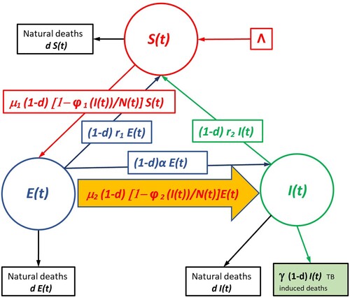
The fraction of susceptibles that escape the infection at time t is $(1-d){\mu }_1{\phi }_1\left(I\right(t\left)/N\right)$ where ${\phi }_1\left(I/N\right)$ is the escape function, and ${\mu }_1$, $0\le {\mu }_1<1$ is the level of infection. It is known that even after heavy exposure to TB, some individuals do not develop M. tuberculosis infection and innate immunity probably account for this natural protection or early clearance of M. tuberculosis. BCG vaccination also appears to play a significant role [14]. Therefore, asymptotically, this fraction is bounded below by $(1-d)(1-{\mu }_1)$. Hence in the same time interval, the fraction of susceptibles that did not escape from the infection is $(1-d){\mu }_1(1-\phi (I/N\left)\right)$ (see the Flowchart Figure 1).

The term ${\mu }_2(1-d){\phi }_2\left(I\right(t\left)/N\right(t\left)\right)$ models the exogenous reinfection rates with ${\mu }_2$ representing the level of reinfection, $0\le {\mu }_2\le 1$. About 5–10 % of infected people, Mtb can be reactivated and propagated to transmit TB [14]. When there is no exogenous infection, we have ${\mu }_2=0$, and the system reduces to (2) $\begin{array}{rl}S(t+1)& =\mathrm{\Lambda }+(1-{\mu }_1)(1-d)S\left(t\right)+{\mu }_1(1-d){\phi }_1\left(I\right(t\left)/N\right(t\left)\right)S\left(t\right)+r_1(1-d)E\left(t\right)\\ & +r_2(1-d)I\left(t\right)\\ E(t+1)& ={\mu }_1(1-d)(1-{\phi }_1(I\left(t\right)/N\left(t\right)\left)\right)S\left(t\right)+(1-d)(1-\alpha -r_1)E\left(t\right)\\ I(t+1)& =(1-d)\mathrm{\alpha E}\left(t\right)+(1-d)(1-\gamma -r_2)I\left(t\right)\end{array}$(2) The flowchart of both models is displayed in Figure 1.

Now $N(t+1)=\mathrm{\Lambda }+(1-d)N\left(t\right)-\gamma (1-d)I$. Then $0<N\left(t\right)\le \frac{\mathrm{\Lambda }}{d}$ and if we assume that $\gamma =0$, then $N\left(t\right)\to \frac{\mathrm{\Lambda }}{d}$ as $t\to \mathrm{\infty }$.

We now make the following two assumptions:

• $A_1:0<\alpha +r_1+{\mu }_2<1,0\le {\mu }_1<1,0<\gamma +r_2<1,0\le d<1$

• $A_2$: We assume that the functions ${\phi }_i\left(I/N\right)$ satisfies the following assumptions:

1. ${\phi }_i\left(I\right(t\left)/N\right(t\left)\right)$ is continuously differentiable for $I\left(t\right)\ge 0$.

2. $0\le {\phi }_i\le 1$, for $I\left(t\right)\ge 0$.

3. ${\phi }_i\left(0\right)=1$, ${\phi }_i^{\mathrm{\prime }}\left(I\right(t\left)/N\right(t\left)\right)<0$ for $I\left(t\right)\ge 0$.

In [15], the contact between susceptibles and infected individuals is assumed to be a Poisson process given by ${\phi }_i\left(I\right(t\left)/N\right)=e^{-{\text{β}}_{i}I\left(t\right)/N\left(t\right)}$, ${\text{β}}_i>0$, i = 1, 2, where ${\text{β}}_i$ is called the transmission coefficient which will be used here.

Let us recall that the threshold parameter ${\mathcal{R}}_0$ is called the net reproduction number (or basic reproduction number or ratio) and is defined as the expected number of infections produced by a single infectious individual introduced into a susceptible population. Consequently, when ${\mathcal{R}}_0<1$, it is expected to imply that the number of infections will decrease over time and the disease will eventually die out. However, when ${\mathcal{R}}_0>1$, a disease outbreak will occur.

3. Endogenous (non-exogenous) SEI compartmental model (with no treatment)

3.1. Net reproduction number ${\mathcal{R}}_0$

To compute the traditional reproduction number ${\mathcal{R}}_0$ we are going to use the next-generation matrix approach [15]. We remind that in the non-exogenous case ${\mu }_2=0$.

Let $X_0=(E,I{)}^T$, $X_1=S^T$, $X=(X_0,X_1)\in R_{+}^3$. Hence system (2(2) $\begin{array}{rl}S(t+1)& =\mathrm{\Lambda }+(1-{\mu }_1)(1-d)S\left(t\right)+{\mu }_1(1-d){\phi }_1\left(I\right(t\left)/N\right(t\left)\right)S\left(t\right)+r_1(1-d)E\left(t\right)\\ & +r_2(1-d)I\left(t\right)\\ E(t+1)& ={\mu }_1(1-d)(1-{\phi }_1(I\left(t\right)/N\left(t\right)\left)\right)S\left(t\right)+(1-d)(1-\alpha -r_1)E\left(t\right)\\ I(t+1)& =(1-d)\mathrm{\alpha E}\left(t\right)+(1-d)(1-\gamma -r_2)I\left(t\right)\end{array}$(2) ) may be written as (3) $\begin{array}{rl}{X}_0(t+1)& =G_0\left(X\right(t\left)\right)\\ X_1(t+1)& =G_1\left(X\right(t\left)\right)\end{array}$(3) where $G_0\left(X\right(t\left)\right)=\left(\begin{array}{c}E(t+1)\\ I(t+1)\end{array}\right)=\mathcal{F}\left(t\right)+\mathcal{T}\left(t\right)$, and $G_1\left(X\right(t\left)\right)=S(t+1)$, where $\mathcal{F}\left(t\right)=\left(\begin{array}{c}{\mu }_1(1-d)(1-{\phi }_1(I\left(t\right)/N\left(t\right)\left)S\right(t)\\ 0\end{array}\right)=\left(\begin{array}{c}{\mathcal{F}}_1\left(t\right)\\ {\mathcal{F}}_2\left(t\right)\end{array}\right)$is the vector of new infections that survive in the time interval $[0,t]$, and $\mathcal{T}\left(t\right)=\left(\begin{array}{c}(1-d)(1-\alpha -r_1)E\left(t\right)\\ \alpha (1-d)E\left(t\right)+(1-d)(1-\gamma -r_2)I\left(t\right)\end{array}\right)=\left(\begin{array}{c}{\mathcal{T}}_1\left(t\right)\\ {\mathcal{T}}_2\left(t\right)\end{array}\right)$is the vector of all other transitions.

Next, we compute the Jacobian matrix of $\mathcal{T}\left(t\right)$ and $\mathcal{F}\left(t\right)$ at the disease-free equilibrium (DFE) ${\mathcal{E}}_0=(0,0,S^{\ast })=(0,0,N^{\ast })$ $\begin{array}{rl}F\left(t\right){|}_{(0,0,S^{\ast })}& =\left(\begin{array}{cc}{\displaystyle \frac{\mathrm{\partial }{\mathcal{F}}_1\left(t\right)}{\mathrm{\partial }E}}& {\displaystyle \frac{\mathrm{\partial }{\mathcal{F}}_1\left(t\right)}{\mathrm{\partial }I}}\\ {\displaystyle \frac{\mathrm{\partial }{\mathcal{F}}_2\left(t\right)}{\mathrm{\partial }E}}& {\displaystyle \frac{\mathrm{\partial }{\mathcal{F}}_2\left(t\right)}{\mathrm{\partial }I}}\end{array}\right)=\left(\begin{array}{cc}0& {\mu }_1{\text{β}}_1(1-d)\\ 0& 0\end{array}\right)\\ T\left(t\right){|}_{(0,0,S^{\ast })}& =\left(\begin{array}{cc}{\displaystyle \frac{\mathrm{\partial }{\mathcal{T}}_1\left(t\right)}{\mathrm{\partial }E}}& {\displaystyle \frac{\mathrm{\partial }{\mathcal{T}}_1\left(t\right)}{\mathrm{\partial }I}}\\ {\displaystyle \frac{\mathrm{\partial }{\mathcal{T}}_2\left(t\right)}{\mathrm{\partial }E}}& {\displaystyle \frac{\mathrm{\partial }{\mathcal{T}}_2\left(t\right)}{\mathrm{\delta I}}}\end{array}\right)=\left(\begin{array}{cc}1-d\left)\right(1-\alpha -r_1)& 0\\ \alpha (1-d)& (1-d)(1-\gamma -r_2)\end{array}\right).\end{array}$Now the basic reproduction number is given by ${\mathcal{R}}_0\left({\mathcal{E}}_0\right)=\rho \left(\right(F(I-T){)}^{-1})$, where ρ denotes the spectral radius of a matrix [15–17]. $\begin{array}{rl}F(I-T{)}^{-1}& =(\begin{array}{c}{\displaystyle \frac{{\mu }_1\alpha {\text{β}}_1(1-d)}{(1-(1-d\left)\right(1-\alpha -r_1\left)\right)(1-(1-d\left)\right(1-\gamma -r_2\left)\right)}}\\ 0\end{array}\\ & \begin{array}{c}{\displaystyle \frac{{\mu }_1{\text{β}}_1(1-d)}{1-(1-d)(1-\gamma -r_2)}}\\ 0\end{array}).\end{array}$Hence (4) ${\mathcal{R}}_0\left({\mathcal{E}}_0\right)=\frac{{\mu }_1\alpha {\text{β}}_1(1-d)}{(1-(1-d\left)\right(1-\alpha -r_1\left)\right)(1-(1-d\left)\right(1-\gamma -r_2\left)\right)}.$(4)

3.2. Local stability of DFE of the endogenous model

Theorem 3.1

The DFE $\left({\mathcal{E}}_0\right)$ of system (2(2) $\begin{array}{rl}S(t+1)& =\mathrm{\Lambda }+(1-{\mu }_1)(1-d)S\left(t\right)+{\mu }_1(1-d){\phi }_1\left(I\right(t\left)/N\right(t\left)\right)S\left(t\right)+r_1(1-d)E\left(t\right)\\ & +r_2(1-d)I\left(t\right)\\ E(t+1)& ={\mu }_1(1-d)(1-{\phi }_1(I\left(t\right)/N\left(t\right)\left)\right)S\left(t\right)+(1-d)(1-\alpha -r_1)E\left(t\right)\\ I(t+1)& =(1-d)\mathrm{\alpha E}\left(t\right)+(1-d)(1-\gamma -r_2)I\left(t\right)\end{array}$(2) ) is locally asymptotically stable if ${\mathcal{R}}_0\left({\mathcal{E}}_0\right)<1$ and a saddle if ${\mathcal{R}}_0\left({\mathcal{E}}_0\right)>1$.

Proof.

Jacobian matrix of system (2(2) $\begin{array}{rl}S(t+1)& =\mathrm{\Lambda }+(1-{\mu }_1)(1-d)S\left(t\right)+{\mu }_1(1-d){\phi }_1\left(I\right(t\left)/N\right(t\left)\right)S\left(t\right)+r_1(1-d)E\left(t\right)\\ & +r_2(1-d)I\left(t\right)\\ E(t+1)& ={\mu }_1(1-d)(1-{\phi }_1(I\left(t\right)/N\left(t\right)\left)\right)S\left(t\right)+(1-d)(1-\alpha -r_1)E\left(t\right)\\ I(t+1)& =(1-d)\mathrm{\alpha E}\left(t\right)+(1-d)(1-\gamma -r_2)I\left(t\right)\end{array}$(2) ) at ${\mathcal{E}}_0$ represented by $J\left({\mathcal{E}}_0\right)$ is given by (5) $J\left({\mathcal{E}}_0\right)=\left(\begin{array}{ccc}1-d& r_1(1-d)& r_2(1-d)-{\mu }_1{\text{β}}_1\\ 0& (1-d)(1-\alpha -r_1)& {\mu }_1{\text{β}}_1(1-d)\\ 0& \alpha (1-d)& (1-d)(1-\gamma -r_2)\end{array}\right)$(5) The first eigenvalue of the Jacobian matrix is ${\lambda }_1=1-d<1$. The remaining two eigenvalues are the eigenvalues of the matrix (6) $A=\left(\begin{array}{cc}(1-d)(1-\alpha -r_1)& {\mu }_1{\text{β}}_1(1-d)\\ \alpha (1-d)& (1-d)(1-\gamma -r_2)\end{array}\right),$(6) We now use the determinant-trace criteria to show that the two eigenvalues of this matrix lie inside the unit disk [18,19].

Now determinant $\det \left(A\right)=(1-d{)}^2(1-\alpha -r_1\left)\right(1-\gamma -r_2)-{\mu }_1\alpha {\text{β}}_1(1-d{)}^2$, and trace $\mathrm{tr}\left(A\right)=(1-d)(1-\alpha -r_1)+(1-d)(1-\gamma -r_2)$

Since ${\mathcal{R}}_0\left({\mathcal{E}}_0\right)<1$, it follows that $\det \left(A\right)<1$.

Moreover, $\det \left(A\right)>\mathrm{tr}\left(A\right)-1$. Since $\mathrm{tr}\left(A\right)>0$, $\det \left(A\right)>|\mathrm{tr}\left(A\right)|-1$.

Hence, all the eigenvalues of the Jacobian matrix are inside the unit disk; thus, the DFE is locally asymptotically stable.

Next, we consider the case when ${\mathcal{R}}_0=1$. In this case, the first eigenvalue is ${\lambda }_1=1-d<1$. Now $\det \left(A\right)=\mathrm{tr}\left(A\right)-1$. By Theorem (4.5) in [19], the remaining two eigenvalues are ${\lambda }_2=1$ and ${\lambda }_3=\det \left(A\right)=\mathrm{tr}\left(A\right)-1=(1-d)(1-(\alpha +r_1)+1-(\gamma +r_2\left)\right)-1$. Hence $|{\lambda }_3|<1$. Thus at ${\mathcal{R}}_0=1$, the system would go through transcritical bifurcation or exchange of stability.

If ${\mathcal{R}}_0>1$, then one may show that $\det \left(A\right)<\mathrm{tr}\left(A\right)-1$, and $\det \left(A\right)>-\mathrm{tr}\left(A\right)-1$. Hence, the DFE is unstable. More precisely, the DFE is a saddle since ${\lambda }_1=1-d<1$, ${\lambda }_2>1$, and $0<{\lambda }_3<1$.

3.3. Global stability of DFE of the endogenous system via Liapunov functions

In this section, we are going to use the LaSalle invariance theorem [18,20] stated below.

Theorem 3.2

LaSalle Invariance Principle

Consider the difference equation (7) $\mathbf{x}(t+1)=F\left(\mathbf{x}\right(t\left)\right)$(7) where $F:{\mathbb{R}}_{+}^n\to {\mathbb{R}}_{+}^n$ is continuous on a subset G of ${\mathbb{R}}_{+}^n$. Suppose there is a Liapunov function $V:G\to \mathbb{R}$ such that V is continuous on the closure $\overline{G}$ of G. Let $E=\{\mathbf{x}:\mathrm{\Delta V}(\mathbf{x}\left(t\right))=0\}$ and M be the largest positively invariant subset of E. Assume that for every point $\mathbf{x}\in G$, its orbit $O\left(\mathbf{x}\right)$ is bounded and is a subset of G. Then there exists $c\in R$ such that for every $x\in G$, $\omega \left(x\right)\subset M\cap V^{-1}\left(c\right)$.

Consider the equation $X_1(t+1)=G_1(0,x_1(t\left)\right)=\mathrm{\Lambda }+(1-d)S\left(t\right)$ The equilibrium point $X_1^{\ast }=\frac{\mathrm{\Lambda }}{d}$ is globally asymptotically stable since

$\underset{t\to \mathrm{\infty }}{lim}S\left(t\right)=\underset{t\to \mathrm{\infty }}{lim}(1-d{)}^t(S_0-\frac{\mathrm{\Lambda }}{d})+\frac{\mathrm{\Lambda }}{d}=\frac{\mathrm{\Lambda }}{d}$ Consider the matrix $B=(I-T{)}^{-1}F$Then $\lambda =\frac{\alpha {\text{β}}_1{\mu }_1}{(1-(1-d\left)\right(1-\alpha -r_1\left)\right)(1-(1-d\left)\right(1-\gamma -r_2\left)\right)}$ is an eigenvalue of B. The corresponding eigenvector of B is given by $W=(1,\frac{\alpha (1-d)}{1-(1-d)(1-\gamma -r_2)}{)}^T$. Define a Liapunov function as $V(X_0,X_1)=W^T(I-T{)}^{-1}{X}_0$with $X_0\in {\mathbf{R}}_{+}^2\left|\right\{0\}$.

Now let $\mathbf{f}(X_0,X_1)=(F+T)X_0-G_0(X_0,X_1)$. Then $X_0(t+1)=(F+T)X_0\left(t\right)-\mathbf{f}\left(X_0\right(t),X_1(t\left)\right)$ since $G_0(0,X_1^{\ast })=0$, $\mathbf{f}(0,X_1^{\ast })=\mathbf{0}$.

Theorem 3.3

Assume that ${\mathcal{R}}_0\le 1$. Then the disease-free equilibrium $X^{\ast }=(0,X_1^{\ast })$ of the endogenous system (2(2) $\begin{array}{rl}S(t+1)& =\mathrm{\Lambda }+(1-{\mu }_1)(1-d)S\left(t\right)+{\mu }_1(1-d){\phi }_1\left(I\right(t\left)/N\right(t\left)\right)S\left(t\right)+r_1(1-d)E\left(t\right)\\ & +r_2(1-d)I\left(t\right)\\ E(t+1)& ={\mu }_1(1-d)(1-{\phi }_1(I\left(t\right)/N\left(t\right)\left)\right)S\left(t\right)+(1-d)(1-\alpha -r_1)E\left(t\right)\\ I(t+1)& =(1-d)\mathrm{\alpha E}\left(t\right)+(1-d)(1-\gamma -r_2)I\left(t\right)\end{array}$(2) ) is globally asymptotically stable.

Proof.

Now $\begin{array}{rl}\mathrm{\Delta V}(X_0,X_1)& =V\left(G_0\right(X_0,X_1),G_1(X_0,X_1\left)\right)-V(X_0,X_1)\\ & =W^T(I-T{)}^{-1}{X}_0(t+1)-W^T(I-T{)}^{-1}{X}_0\left(t\right)\\ & =W^T(I-T{)}^{-1}(F+t\left)X_0\right(t)-W^T(I-T{)}^{-1}\mathbf{f}\left(X_0\right(t),X_1(t\left)\right)\\ & -W^T(I-T{)}^{-1}{X}_0(t)\\ & =W^T(I-T{)}^{-1}(T-I+F+I\left)X_0\right(t)-W^T(I-T{)}^{-1}\mathbf{f}\left(X_0\right(t),X_1(t\left)\right)\\ & -W^T(I-T{)}^{-1}{X}_0(t)\\ & =W^T(-1+{\mathcal{R}}_0)X_0\left(t\right)-W^T(I-T{)}^{-1}\mathbf{f}(X_0\left(t\right),X_1\left(t\right))\end{array}$since ${\mathcal{R}}_0\le 1$ and $W^T(I-T{)}^{-1}f(X_0\left(t\right),X_1\left(t\right))\ge 0$. It follows that $\mathrm{\Delta V}(X_0,X_1)\le 0$.

By the LaSalle Invariance Principle, $X\left(t\right)=\left(\begin{array}{c}{X}_0\left(t\right)\\ X_1\left(t\right)\end{array}\right)$ approaches the largest positively invariant subset M of the set $E=\{X\in {\mathbb{R}}_{+}^3|\mathrm{\Delta V}(X)=0\}$, where $M=\left\{\right(0,X_1)|X_1\in {\mathbb{R}}_{+}^2\}$. Hence the only invariant set M is the disease-free equilibrium $(0,X_1^{\ast }{)}^T$. Therefore the disease-free equilibrium is globally asymptotically stable. Hence the only invariant set in M is the disease-free equilibrium $(0,X_1^{\ast }{)}^T$. Therefore the disease-free equilibrium is globally asymptotically stable.

Remark 3.4

It should be noted that global stability when ${\mathcal{R}}_0<1$ was proved in [21].

4. Existence and uniqueness of the endemic equilibrium of the endogenous model

4.1. case $\gamma =0$, $r_1=r_2=0$

4.1.1. Existence

In this section, we investigate the dynamics of the endogenous model (2(2) $\begin{array}{rl}S(t+1)& =\mathrm{\Lambda }+(1-{\mu }_1)(1-d)S\left(t\right)+{\mu }_1(1-d){\phi }_1\left(I\right(t\left)/N\right(t\left)\right)S\left(t\right)+r_1(1-d)E\left(t\right)\\ & +r_2(1-d)I\left(t\right)\\ E(t+1)& ={\mu }_1(1-d)(1-{\phi }_1(I\left(t\right)/N\left(t\right)\left)\right)S\left(t\right)+(1-d)(1-\alpha -r_1)E\left(t\right)\\ I(t+1)& =(1-d)\mathrm{\alpha E}\left(t\right)+(1-d)(1-\gamma -r_2)I\left(t\right)\end{array}$(2) ) with $\gamma =0$. In this case $\underset{t\to \mathrm{\infty }}{lim}N\left(t\right)=N^{\ast }=\mathrm{\Lambda }/d$. Then System (2(2) $\begin{array}{rl}S(t+1)& =\mathrm{\Lambda }+(1-{\mu }_1)(1-d)S\left(t\right)+{\mu }_1(1-d){\phi }_1\left(I\right(t\left)/N\right(t\left)\right)S\left(t\right)+r_1(1-d)E\left(t\right)\\ & +r_2(1-d)I\left(t\right)\\ E(t+1)& ={\mu }_1(1-d)(1-{\phi }_1(I\left(t\right)/N\left(t\right)\left)\right)S\left(t\right)+(1-d)(1-\alpha -r_1)E\left(t\right)\\ I(t+1)& =(1-d)\mathrm{\alpha E}\left(t\right)+(1-d)(1-\gamma -r_2)I\left(t\right)\end{array}$(2) ) becomes (8) $\begin{array}{r}\begin{array}{rl}S(t+1)& =\mathrm{\Lambda }+(1-{\mu }_1)(1-d)S\left(t\right)+{\mu }_1(1-d){\phi }_1\left(I\right(t\left)/N\right(t\left)\right)S\left(t\right)+r_1(1-d)E\left(t\right)\\ & +r_2(1-d)I\left(t\right)\\ E(t+1)& ={\mu }_1(1-d)(1-{\phi }_1(I\left(t\right)/N\left(t\right)\left)\right)S\left(t\right)+(1-d)(1-\alpha -r_1)E\left(t\right)\\ I(t+1)& =(1-d)\mathrm{\alpha E}\left(t\right)+(1-d)(1-r_2)I\left(t\right)\end{array}\end{array}$(8) This system is asymptotic to the following system, where $N\left(t\right)$ is replaced by $N^{\ast }$. (9) $\begin{array}{rl}S(t+1)& =\mathrm{\Lambda }+(1-{\mu }_1)(1-d)S\left(t\right)+{\mu }_1(1-d){\phi }_1\left(I\right(t\left)/N^{\ast }\right)S\left(t\right)+r_1(1-d)E\left(t\right)\\ & +r_2(1-d)I\left(t\right)\\ E(t+1)& ={\mu }_1(1-d)(1-{\phi }_1(I\left(t\right)/N^{\ast }\left)S\right(t)+(1-d\left)\right(1-\alpha -r_1\left)E\right(t)\\ I(t+1)& =(1-d)\mathrm{\alpha E}\left(t\right)+(1-d)(1-r_2)I\left(t\right)\end{array}$(9) We will now focus our attention on the analysis of System (9(9) $\begin{array}{rl}S(t+1)& =\mathrm{\Lambda }+(1-{\mu }_1)(1-d)S\left(t\right)+{\mu }_1(1-d){\phi }_1\left(I\right(t\left)/N^{\ast }\right)S\left(t\right)+r_1(1-d)E\left(t\right)\\ & +r_2(1-d)I\left(t\right)\\ E(t+1)& ={\mu }_1(1-d)(1-{\phi }_1(I\left(t\right)/N^{\ast }\left)S\right(t)+(1-d\left)\right(1-\alpha -r_1\left)E\right(t)\\ I(t+1)& =(1-d)\mathrm{\alpha E}\left(t\right)+(1-d)(1-r_2)I\left(t\right)\end{array}$(9) )

Proposition 4.1

Assume that $r_1=r_2=0$, and $\gamma =0$. Then every equilibrium point ${\mathcal{E}}^{\ast }=(S^{\ast },E^{\ast },I^{\ast }$) of model (9(9) $\begin{array}{rl}S(t+1)& =\mathrm{\Lambda }+(1-{\mu }_1)(1-d)S\left(t\right)+{\mu }_1(1-d){\phi }_1\left(I\right(t\left)/N^{\ast }\right)S\left(t\right)+r_1(1-d)E\left(t\right)\\ & +r_2(1-d)I\left(t\right)\\ E(t+1)& ={\mu }_1(1-d)(1-{\phi }_1(I\left(t\right)/N^{\ast }\left)S\right(t)+(1-d\left)\right(1-\alpha -r_1\left)E\right(t)\\ I(t+1)& =(1-d)\mathrm{\alpha E}\left(t\right)+(1-d)(1-r_2)I\left(t\right)\end{array}$(9) ) is of the form ${\mathcal{E}}^{\ast }=(S^{\ast },\frac{\mathrm{\Lambda }-d{S}^{\ast }}{(d+\alpha -\mathrm{\alpha d})},\frac{(1-d)\alpha (\mathrm{\Lambda }-d{S}^{\ast })}{d(d+\alpha -\mathrm{\alpha d})})$ with $S^{\ast }$ solution of (10) $d(d+\alpha -\mathrm{\alpha d})N^{\ast }\ln \left[\frac{(1-d){\mu }_1{S}^{\ast }}{({\mu }_1+d-{\mu }_{1}d)S^{\ast }-\mathrm{\Lambda }}\right]+(1-d)\alpha {\text{β}}_{1}d{S}^{\ast }=(1-d)\alpha {\text{β}}_1\mathrm{\Lambda },$(10) This equation can also be written as (11) $\begin{array}{rl}& d(d+\alpha -\mathrm{\alpha d})N^{\ast }[(1-d)\ln \left(S^{\ast }\right)-\ln \left[\right({\mu }_1+d-{\mu }_{1}d)S^{\ast }-\mathrm{\Lambda }]]+(1-d)\alpha {\text{β}}_{1}d{S}^{\ast }\\ & =(1-d)\alpha {\text{β}}_1\mathrm{\Lambda }-d(d+\alpha +\mathrm{\alpha d})N^{\ast }\ln \left(\right(1-d\left){\mu }_1\right),\end{array}$(11)

Proof.

Consider $S(t+1)=\mathrm{\Lambda }+(1-{\mu }_1)(1-d)S\left(t\right)+{\mu }_1(1-d){\mathrm{e}}^{-{\text{β}}_1\left(I\right(t\left)/N^{\ast }\right)}S\left(t\right)$when $S(t+1)=S\left(t\right)$,

one has: (12) $(1-d){\mu }_1{\mathrm{e}}^{-{\text{β}}_1\frac{I^{\ast }}{N^{\ast }}}{S}^{\ast }=-\mathrm{\Lambda }+({\mu }_1+d-{\mu }_{1}d)S^{\ast }$(12) then if ${\mu }_1>0$, ${\text{β}}_1>0$ and $S^{\ast }>0$ ${\mathrm{e}}^{-{\text{β}}_1\frac{I^{\ast }}{N^{\ast }}}=\frac{-\mathrm{\Lambda }+({\mu }_1+d-{\mu }_{1}d)S^{\ast }}{(1-d){\mu }_1{S}^{\ast }}$or (13) $\begin{array}{rl}& \ln \left[{\mathrm{e}}^{-{\text{β}}_1\frac{I^{\ast }}{N^{\ast }}}\right]=\ln \left[\frac{-\mathrm{\Lambda }+({\mu }_1+d-{\mu }_{1}d)S^{\ast }}{(1-d){\mu }_1{S}^{\ast }}\right]\\ & -{\text{β}}_1\frac{I^{\ast }}{N^{\ast }}=\ln \left[\frac{-\mathrm{\Lambda }+({\mu }_1+d-{\mu }_{1}d)S^{\ast }}{(1-d){\mu }_1{S}^{\ast }}\right]\\ & I^{\ast }=-\frac{N^{\ast }}{{\text{β}}_1}\ln \left[\frac{-\mathrm{\Lambda }+({\mu }_1+d-{\mu }_{1}d)S^{\ast }}{(1-d){\mu }_1{S}^{\ast }}\right]\end{array}$(13) Consider now $E(t+1)=(1-d){\mu }_1(1-{\mathrm{e}}^{-{\text{β}}_1\left(I\right(t\left)/N^{\ast }\right)})S\left(t\right)+(1-d)(1-\alpha )E\left(t\right)$when $E(t+1)=E\left(t\right)$, one has: $0={\mu }_1(1-d)(1-{\mathrm{e}}^{-{\text{β}}_1\frac{I^{\ast }}{N^{\ast }}})S^{\ast }-(d+\alpha -\mathrm{\alpha d})E^{\ast }$From (12(12) $(1-d){\mu }_1{\mathrm{e}}^{-{\text{β}}_1\frac{I^{\ast }}{N^{\ast }}}{S}^{\ast }=-\mathrm{\Lambda }+({\mu }_1+d-{\mu }_{1}d)S^{\ast }$(12) ) it comes: (14) $\begin{array}{rl}& 0={\mu }_1{S}^{\ast }+\mathrm{\Lambda }-{\mu }_1{S}^{\ast }-d{S}^{\ast }-(d+\alpha -\mathrm{\alpha d})E^{\ast }\\ & (d+\alpha -\mathrm{\alpha d})E^{\ast }=\mathrm{\Lambda }-\mathrm{d}{S}^{\ast }\\ & E^{\ast }=\frac{\mathrm{\Lambda }-\mathrm{d}{S}^{\ast }}{(d+\alpha -\mathrm{\alpha d})}\end{array}$(14) Consider now $I(t+1)=(1-d)\mathrm{\alpha E}\left(t\right)+(1-d)I\left(t\right)$when $I(t+1)=I\left(t\right)$, one has: (15) $\begin{array}{rl}& 0=(1-d)\alpha E^{\ast }-d{I}^{\ast }\\ & I^{\ast }=\frac{(1-d)\alpha E^{\ast }}{d}\\ & I^{\ast }=\frac{(1-d)\alpha (\mathrm{\Lambda }-d{S}^{\ast })}{d(d+\alpha -\mathrm{\alpha d})}\end{array}$(15) Equaling (15(15) $\begin{array}{rl}& 0=(1-d)\alpha E^{\ast }-d{I}^{\ast }\\ & I^{\ast }=\frac{(1-d)\alpha E^{\ast }}{d}\\ & I^{\ast }=\frac{(1-d)\alpha (\mathrm{\Lambda }-d{S}^{\ast })}{d(d+\alpha -\mathrm{\alpha d})}\end{array}$(15) ) to (13(13) $\begin{array}{rl}& \ln \left[{\mathrm{e}}^{-{\text{β}}_1\frac{I^{\ast }}{N^{\ast }}}\right]=\ln \left[\frac{-\mathrm{\Lambda }+({\mu }_1+d-{\mu }_{1}d)S^{\ast }}{(1-d){\mu }_1{S}^{\ast }}\right]\\ & -{\text{β}}_1\frac{I^{\ast }}{N^{\ast }}=\ln \left[\frac{-\mathrm{\Lambda }+({\mu }_1+d-{\mu }_{1}d)S^{\ast }}{(1-d){\mu }_1{S}^{\ast }}\right]\\ & I^{\ast }=-\frac{N^{\ast }}{{\text{β}}_1}\ln \left[\frac{-\mathrm{\Lambda }+({\mu }_1+d-{\mu }_{1}d)S^{\ast }}{(1-d){\mu }_1{S}^{\ast }}\right]\end{array}$(13) ) it comes $d(d+\alpha -\mathrm{\alpha d})N^{\ast }\ln \left[\frac{(1-d){\mu }_1{S}^{\ast }}{({\mu }_1+d-{\mu }_{1}d)S^{\ast }-\mathrm{\Lambda }}\right]+(1-d)\alpha {\text{β}}_{1}d{S}^{\ast }=(1-d)\alpha {\text{β}}_1\mathrm{\Lambda },$

4.1.2. Uniqueness

Theorem 4.2

Assume that $r_1=r_2=0$, $\gamma =0$ and ${\mathcal{R}}_0>1$. Then there exists a unique endemic equilibrium point ${\mathcal{E}}^{\ast }=(S^{\ast },E^{\ast },I^{\ast })$ of System (9(9) $\begin{array}{rl}S(t+1)& =\mathrm{\Lambda }+(1-{\mu }_1)(1-d)S\left(t\right)+{\mu }_1(1-d){\phi }_1\left(I\right(t\left)/N^{\ast }\right)S\left(t\right)+r_1(1-d)E\left(t\right)\\ & +r_2(1-d)I\left(t\right)\\ E(t+1)& ={\mu }_1(1-d)(1-{\phi }_1(I\left(t\right)/N^{\ast }\left)S\right(t)+(1-d\left)\right(1-\alpha -r_1\left)E\right(t)\\ I(t+1)& =(1-d)\mathrm{\alpha E}\left(t\right)+(1-d)(1-r_2)I\left(t\right)\end{array}$(9) )

Proof.

Consider the function (16) $f\left(x\right)=d(d+\alpha -\mathrm{\alpha d})N^{\ast }\ln \left[\frac{(1-d){\mu }_{1}x}{({\mu }_1+d-{\mu }_{1}d)x-\mathrm{\Lambda }}\right]+(1-d)\alpha {\text{β}}_1\mathrm{d}x,$(16) which is only defined for $x>\frac{\mathrm{\Lambda }}{{\mu }_1+d-{\mu }_{1}d}$.

Its derivative is: (17) $f^{\mathrm{\prime }}\left(x\right)=-\frac{d(d+\alpha -\mathrm{\alpha d})N^{\ast }\mathrm{\Lambda }}{x\left[\right({\mu }_1+d-{\mu }_{1}d)x-\mathrm{\Lambda }]}+(1-d)\alpha {\text{β}}_{1}d,$(17) and its second derivative is: (18) $f^{\mathrm{\prime \prime }}\left(x\right)=\frac{d(d+\alpha -\mathrm{\alpha d})N^{\ast }\mathrm{\Lambda }\left[2\right({\mu }_1+d-{\mu }_{1}d)x-\mathrm{\Lambda }]}{x^2{\left[\right({\mu }_1+d-{\mu }_{1}d)x-\mathrm{\Lambda }]}^2},$(18) which is always positive because from (11(11) $\begin{array}{rl}& d(d+\alpha -\mathrm{\alpha d})N^{\ast }[(1-d)\ln \left(S^{\ast }\right)-\ln \left[\right({\mu }_1+d-{\mu }_{1}d)S^{\ast }-\mathrm{\Lambda }]]+(1-d)\alpha {\text{β}}_{1}d{S}^{\ast }\\ & =(1-d)\alpha {\text{β}}_1\mathrm{\Lambda }-d(d+\alpha +\mathrm{\alpha d})N^{\ast }\ln \left(\right(1-d\left){\mu }_1\right),\end{array}$(11) ) $({\mu }_1+d-{\mu }_{1}d)S^{\ast }-\mathrm{\Lambda }>0$, i.e. $({\mu }_1+d-{\mu }_{1}d)x-\mathrm{\Lambda }>0$, hence $\mathrm{\Lambda }<({\mu }_1+d-{\mu }_{1}d)x<2({\mu }_1+d-{\mu }_{1}d)x$ In addition $0\le \alpha <1$ and $0\le d<1$ implies that $\mathrm{\alpha d}<d$ hence $d+\alpha -\mathrm{\alpha d}>0$. Therefore $f\left(x\right)$ is convex and $f^{\mathrm{\prime }}\left(x\right)$ is always increasing.

The equation (19) $f\left(x\right)=(1-d)\alpha {\text{β}}_1\mathrm{\Lambda },$(19) which represents the intersection of a convex curve with and horizontal straight line, and can have either zero, one, or two solutions. Clearly, $x=N^{\ast }$ satisfies equation (19(19) $f\left(x\right)=(1-d)\alpha {\text{β}}_1\mathrm{\Lambda },$(19) ), which gives us the disease equilibrium point $(S^{\ast },0,0)$. Therefore this equation can have only one or two solutions. Moreover, if ${\mathcal{R}}_0=1$, and since $N^{\ast }=\mathrm{\Lambda }/d$, it follows that (20) $f^{\mathrm{\prime }}\left(N^{\ast }\right)=-\frac{d(d+\alpha -\mathrm{\alpha d})d\mathrm{\Lambda }}{{\mu }_1\mathrm{\Lambda }}+d\frac{d(d+\alpha -\mathrm{\alpha d})}{{\mu }_1}=0,$(20) Therefore the tangent to the convex curve is horizontal, and, consequently, there is only one point of intersection between the horizontal line and the curve which is the DFE.

It is easy to verify that if ${\mathcal{R}}_0>1$ or $\alpha \text{β}>\frac{d(d+\alpha )}{\mu }$, then $f^{\mathrm{\prime }}\left(N^{\ast }\right)>0$ and, consequently, there is an equilibrium point on the left-hand side intersection between the convex curve and the horizontal straight line, with $S^{\ast }<N^{\ast }$. This proves the existence and uniqueness of the endemic equilibrium point if ${\mathcal{R}}_0>1$.

4.2. Reproduction number computed using the DFE or the endemic equilibrium

We consider the endogenous model with $\gamma =0$ and ${\phi }_1\left(I\right(t\left)/N^{\ast }\right)=e^{-{\text{β}}_{1}I\left(t\right)/N^{\ast }}$, (21) $\begin{array}{rl}S(t+1)& =\mathrm{\Lambda }+(1-{\mu }_1)(1-d)S\left(t\right)+{\mu }_1(1-d)e^{-{\text{β}}_{i}I\left(t\right)/N^{\ast }}S\left(t\right)+r_1(1-d)E\left(t\right)\\ & +r_2(1-d)I\left(t\right)\\ E(t+1)& ={\mu }_1(1-d)(1-e^{-{\text{β}}_{i}I\left(t\right)/N^{\ast }})S\left(t\right)+(1-d)(1-\alpha -r_1)E\left(t\right)\\ I(t+1)& =\alpha (1-d)E\left(t\right)+(1-d)(1-r_2)I\left(t\right)\end{array}$(21) We are going to use the next-generation matrix approach [15]. Let $X_0=(E,I{)}^T$, $X_1=S^T$, $X=(X_0,X_1)\in R_{+}^3$. Hence system (21(21) $\begin{array}{rl}S(t+1)& =\mathrm{\Lambda }+(1-{\mu }_1)(1-d)S\left(t\right)+{\mu }_1(1-d)e^{-{\text{β}}_{i}I\left(t\right)/N^{\ast }}S\left(t\right)+r_1(1-d)E\left(t\right)\\ & +r_2(1-d)I\left(t\right)\\ E(t+1)& ={\mu }_1(1-d)(1-e^{-{\text{β}}_{i}I\left(t\right)/N^{\ast }})S\left(t\right)+(1-d)(1-\alpha -r_1)E\left(t\right)\\ I(t+1)& =\alpha (1-d)E\left(t\right)+(1-d)(1-r_2)I\left(t\right)\end{array}$(21) ) may be written as (22) $\begin{array}{rl}{X}_0(t+1)& =G_0\left(X\right(t\left)\right)\\ X_1(t+1)& =G_1\left(X\right(t\left)\right)\end{array}$(22) where $G_0\left(X\right(t\left)\right)=\left(\begin{array}{c}E(t+1)\\ I(t+1)\end{array}\right)=\mathcal{F}\left(t\right)+\mathcal{T}\left(t\right)$, and $G_1\left(X\right(t\left)\right)=S(t+1)$, where is the vector of all other transitions. $\mathcal{F}\left(t\right)=\left(\begin{array}{c}{\mu }_1(1-d)\left(\right(1-e^{-{\text{β}}_{i}I\left(t\right)/N^{\ast }}S\left(t\right)\\ 0\end{array}\right)=\left(\begin{array}{c}{\mathcal{F}}_1\left(t\right)\\ {\mathcal{F}}_2\left(t\right)\end{array}\right)$is the vector of new infections that survive in the time interval $[0,t]$, and $\mathcal{T}\left(t\right)=\left(\begin{array}{c}(1-d)(1-r_1-\alpha )E\left(t\right)\\ \alpha (1-d)E\left(t\right)+(1-d)(1-r_2)I\left(t\right)\end{array}\right)=\left(\begin{array}{c}{\mathcal{T}}_1\left(t\right)\\ {\mathcal{T}}_2\left(t\right)\end{array}\right)$Let $T\left(t\right)$ and $F\left(t\right)$ be the Jacobian matrices of $\mathcal{T}\left(t\right)$ and $\mathcal{F}\left(t\right)$, respectively, at the endemic equilibrium ${\mathcal{E}}^{\ast }=(E^{\ast },I^{\ast },S^{\ast })$. Then $\begin{array}{rl}F(I-T{)}^{-1}& =\left(\begin{array}{cc}0& {\displaystyle \frac{(1-d){\mu }_1{\text{β}}_1{e}^{-{\text{β}}_1{I}^{\ast }/N^{\ast }}{S}^{\ast }}{N^{\ast }}}\\ 0& 0\end{array}\right)\\ & \times (\begin{array}{c}{\displaystyle \frac{1}{(1-(1-d\left)\right(1-\alpha -r_1\left)\right)}}\\ {\displaystyle \frac{\alpha }{(1-(1-d\left)\right(1-\alpha -r_1\left)\right)(1-(1-d\left)\right(1-r_2\left)\right)}}\end{array}\\ & \begin{array}{c}0\\ {\displaystyle \frac{1}{1-(1-d)(1-\gamma -r_2)}}\end{array})\\ & =(\begin{array}{c}{\displaystyle \frac{{\mu }_1\alpha {\text{β}}_1(1-d)e^{-{\text{β}}_1{I}^{\ast }/N^{\ast }}{S}^{\ast }}{N^{\ast }(1-(1-d\left)\right(1-\alpha -r_1\left)\right)(1-(1-d\left)\right(1-r_2\left)\right))}}\\ 0\end{array}\\ & \begin{array}{c}{\displaystyle \frac{(1-d){\mu }_1\alpha {\text{β}}_1{e}^{-{\text{β}}_1{I}^{\ast }/N^{\ast }}{S}^{\ast }}{N^{\ast }(1-(1-d\left)\right(1-r_2\left)\right)}}\\ 0\end{array})\end{array}$ (23) $\begin{array}{rl}{\mathcal{R}}_0\left({\mathcal{E}}^{\ast }\right)& =\frac{(1-d){\mu }_1\alpha {\text{β}}_1{e}^{-{\text{β}}_1{I}^{\ast }/N^{\ast }}}{N^{\ast }(1-(1-d\left)\right(1-\alpha -r_1\left)\right)(1-(1-d\left)\right(1-r_2\left)\right)}{S}^{\ast }.\end{array}$(23) Using (12(12) $(1-d){\mu }_1{\mathrm{e}}^{-{\text{β}}_1\frac{I^{\ast }}{N^{\ast }}}{S}^{\ast }=-\mathrm{\Lambda }+({\mu }_1+d-{\mu }_{1}d)S^{\ast }$(12) ) it is equivalent to (24) ${\mathcal{R}}_0\left({\mathcal{E}}^{\ast }\right)=\frac{\alpha {\text{β}}_1\left[\right({\mu }_1+d+r_1)S\ast -\mathrm{\Lambda }]}{N^{\ast }(d+\alpha +r_1)(d+\gamma +r_2)}$(24)

Remark 4.3

At the DFE ${\mathcal{E}}_0=(0,0,S^{\ast })$, one has $S^{\ast }=N^{\ast }$, $I^{\ast }=0$, then ${\mathcal{R}}_0\left({\mathcal{E}}_0\right)=\frac{(1-d){\mu }_1\alpha {\text{β}}_1}{(1-(1-d\left)\right(1-\alpha -r_1\left)\right)(1-(1-d\left)\right(1-\gamma -r_2\left)\right)}$ as computed in Section 3.

4.3. Existence and uniqueness in the case $\gamma =0$, $r_1\ne 0,r_2\ne 0$

Next, we are going to use the implicit function theorem for systems to show the existence of the endemic equilibrium in the case $r_1\ne 0$, $r_2\ne 0$, and $\gamma =0$. But before stating the theorem we introduce a few notations and a definition.

Definition 4.4

Let U be an open set in $R^{m+n}$ and suppose that $F;U\to R^n$ is a vector function $F(\mathbf{x},\mathbf{y})$, $F=(F_1,F_2,\dots F_n)$, where $\mathbf{x}=(x_1,x_2\dots x_n)$, $\mathbf{y}=(x_1,x_2\dots y_m)$. We define the $n\times m$ and the $n\times n$ matrices ${\mathrm{\Delta }}_{\mathbf{x}}F$ and ${\mathrm{\Delta }}_{\mathbf{y}}F$ by the formulas ${\mathrm{\Delta }}_{\mathbf{x}}F=\left(\begin{array}{cccc}{\displaystyle \frac{\mathrm{\partial }{F}_1}{\mathrm{\partial }{x}_1}}& {\displaystyle \frac{\mathrm{\partial }{F}_1}{\mathrm{\partial }{x}_2}}& \dots & {\displaystyle \frac{\mathrm{\partial }{F}_1}{\mathrm{\partial }{x}_m}}\\ {\displaystyle \frac{\mathrm{\partial }{F}_2}{\mathrm{\partial }{x}_1}}& {\displaystyle \frac{\mathrm{\partial }{F}_2}{\mathrm{\partial }{x}_2}}& \dots & {\displaystyle \frac{\mathrm{\partial }{F}_2}{\mathrm{\partial }{x}_m}}\\ & & ⋮& \\ {\displaystyle \frac{\mathrm{\partial }{F}_n}{\mathrm{\partial }{x}_1}}& {\displaystyle \frac{\mathrm{\partial }{F}_n}{\mathrm{\partial }{x}_2}}& \dots & {\displaystyle \frac{\mathrm{\partial }{F}_n}{\mathrm{\partial }{x}_m}}\end{array}\right).$

Theorem 4.5

Implicit Function Theorem [22]

Let G be an open set in $R^{m+n}$ containing the point $(\mathbf{a},\mathbf{b})$. Suppose that $F:U\to R^n$ is continuous and has first partial derivatives in G such that $F(\mathbf{a},\mathbf{b})=0$ and $det{\mathrm{\Delta }}_{\mathbf{y}}F(\mathbf{a},\mathbf{b})\ne \mathbf{0}$. Then there exist $\delta >0$ and $\eta >0$ such that for every $\mathbf{x}\in B(\mathbf{a},\delta )$ there exists a unique $\mathbf{y}\in B(\mathbf{b},\eta )$ with $F(\mathbf{x},\mathbf{y})=0$.

5. Local stability of the endemic equilibrium of the endogenous system

Assume that $\gamma =0$. Then $\underset{t\to \mathrm{\infty }}{lim}N\left(t\right)=N^{\ast }=\mathrm{\Lambda }/d$In this case, the endogenous system (2(2) $\begin{array}{rl}S(t+1)& =\mathrm{\Lambda }+(1-{\mu }_1)(1-d)S\left(t\right)+{\mu }_1(1-d){\phi }_1\left(I\right(t\left)/N\right(t\left)\right)S\left(t\right)+r_1(1-d)E\left(t\right)\\ & +r_2(1-d)I\left(t\right)\\ E(t+1)& ={\mu }_1(1-d)(1-{\phi }_1(I\left(t\right)/N\left(t\right)\left)\right)S\left(t\right)+(1-d)(1-\alpha -r_1)E\left(t\right)\\ I(t+1)& =(1-d)\mathrm{\alpha E}\left(t\right)+(1-d)(1-\gamma -r_2)I\left(t\right)\end{array}$(2) ) is asymptotic to the system (25) $\begin{array}{rl}S(t+1)& =\mathrm{\Lambda }+(1-{\mu }_1)(1-d)S\left(t\right)+{\mu }_1(1-d){\phi }_1\left(I\right(t\left)/N^{\ast }\right)S\left(t\right)+r_1(1-d)E\left(t\right)\\ & +r_2(1-d)I\left(t\right)\\ E(t+1)& ={\mu }_1(1-d)(1-{\phi }_1(I\left(t\right)/N^{\ast }\left)\right)S\left(t\right)+(1-d)(1-\alpha -r_1)E\left(t\right)\\ I(t+1)& =\alpha (1-d)E\left(t\right)+(1-d)(1-r_2)I\left(t\right)\end{array}$(25)

Theorem 5.1

Assume that $\gamma =0$ and ${\mathcal{R}}_0\left({\mathcal{E}}^{\ast }\right)<1<{\mathcal{R}}_0\left({\mathcal{E}}_0\right)$. Then for sufficiently small $r_1$ and $r_2$ the endemic equilibrium of the endogenous system (25(25) $\begin{array}{rl}S(t+1)& =\mathrm{\Lambda }+(1-{\mu }_1)(1-d)S\left(t\right)+{\mu }_1(1-d){\phi }_1\left(I\right(t\left)/N^{\ast }\right)S\left(t\right)+r_1(1-d)E\left(t\right)\\ & +r_2(1-d)I\left(t\right)\\ E(t+1)& ={\mu }_1(1-d)(1-{\phi }_1(I\left(t\right)/N^{\ast }\left)\right)S\left(t\right)+(1-d)(1-\alpha -r_1)E\left(t\right)\\ I(t+1)& =\alpha (1-d)E\left(t\right)+(1-d)(1-r_2)I\left(t\right)\end{array}$(25) ) is locally asymptotically stable.

Proof.

The Jacobian matrix of system (2(2) $\begin{array}{rl}S(t+1)& =\mathrm{\Lambda }+(1-{\mu }_1)(1-d)S\left(t\right)+{\mu }_1(1-d){\phi }_1\left(I\right(t\left)/N\right(t\left)\right)S\left(t\right)+r_1(1-d)E\left(t\right)\\ & +r_2(1-d)I\left(t\right)\\ E(t+1)& ={\mu }_1(1-d)(1-{\phi }_1(I\left(t\right)/N\left(t\right)\left)\right)S\left(t\right)+(1-d)(1-\alpha -r_1)E\left(t\right)\\ I(t+1)& =(1-d)\mathrm{\alpha E}\left(t\right)+(1-d)(1-\gamma -r_2)I\left(t\right)\end{array}$(2) ) at ${\mathcal{E}}^{\ast }$ is given by (26) $\begin{array}{rl}B=\mathrm{JF}\left({\mathcal{E}}^{\ast }\right)& =(\begin{array}{cc}(1-{\mu }_1)(1-d)+{\mu }_1(1-d){\mathrm{e}}^{-{\text{β}}_1\frac{I^{\ast }}{N^{\ast }}}& r_1(1-d)\\ {\mu }_1(1-d)(1-{\mathrm{e}}^{-{\text{β}}_1\frac{I^{\ast }}{N^{\ast }}})& (1-d)(1-\alpha -r_1)\\ 0& \alpha (1-d)\end{array}\\ & \begin{array}{c}{r}_2(1-d)-{\displaystyle \frac{{\mu }_1(1-d){\text{β}}_1{S}^{\ast }}{N^{\ast }}}{\mathrm{e}}^{-{\text{β}}_1\frac{I^{\ast }}{N^{\ast }}}\\ {\displaystyle \frac{{\mu }_1(1-d){\text{β}}_1{S}^{\ast }}{N^{\ast }}}{\mathrm{e}}^{-{\text{β}}_1\frac{I^{\ast }}{N^{\ast }}}\\ (1-d)(1-r_2)\end{array}).\end{array}$(26) To find the eigenvalues of $B=\mathrm{JF}\left({\mathcal{E}}^{\ast }\right)$, we solve the characteristic equation $\det (B-\mathrm{\lambda I})=0$ $\begin{array}{rl}& |\begin{array}{cc}(1-{\mu }_1)(1-d)+{\mu }_1(1-d){\mathrm{e}}^{-{\text{β}}_1\frac{I^{\ast }}{N^{\ast }}}-\lambda & r_1(1-d)\\ {\mu }_1(1-d)(1-{\mathrm{e}}^{-{\text{β}}_1\frac{I^{\ast }}{N^{\ast }}})& (1-d)(1-\alpha -r_1)-\lambda \\ 0& \alpha (1-d)\end{array}\\ & \begin{array}{c}{r}_2(1-d)-{\displaystyle \frac{{\mu }_1(1-d){\text{β}}_1{S}^{\ast }}{N^{\ast }}}{\mathrm{e}}^{-{\text{β}}_1\frac{I^{\ast }}{N^{\ast }}}\\ {\displaystyle \frac{{\mu }_1(1-d){\text{β}}_1{S}^{\ast }}{N^{\ast }}}{\mathrm{e}}^{-{\text{β}}_1\frac{I^{\ast }}{N^{\ast }}}\\ (1-d)(1-r_2)-\lambda \end{array}|=0\end{array}$Now adding the first row and the third row to the second row we get $\begin{array}{rl}& |\begin{array}{cc}(1-{\mu }_1)(1-d)+{\mu }_1(1-d){\mathrm{e}}^{-{\text{β}}_1\frac{I^{\ast }}{N^{\ast }}}-\lambda & r_1(1-d)\\ 1-d-\lambda & 1-d-\lambda \\ 0& \alpha (1-d)\end{array}\\ & \begin{array}{c}{r}_2(1-d)-{\displaystyle \frac{{\mu }_1(1-d){\text{β}}_1{S}^{\ast }}{N^{\ast }}}{\mathrm{e}}^{-{\text{β}}_1\frac{I^{\ast }}{N^{\ast }}}\\ 1-d-\lambda \\ (1-d)(1-r_2)-\lambda \end{array}|=0\end{array}$Factoring out $1-d-\lambda$, we see that the first eigenvalue is ${\lambda }_1=1-d<1$. The remaining eigenvalues are solutions to the characteristic equation $\begin{array}{rl}& |\begin{array}{cc}(1-{\mu }_1)(1-d)+{\mu }_1(1-d){\mathrm{e}}^{-{\text{β}}_1\frac{I^{\ast }}{N^{\ast }}}-\lambda & r_1(1-d)\\ 1& 1\\ 0& \alpha (1-d)\end{array}\\ & \begin{array}{c}{r}_2(1-d)-{\displaystyle \frac{{\mu }_1(1-d){\text{β}}_1{S}^{\ast }}{N^{\ast }}}{\mathrm{e}}^{-{\text{β}}_1\frac{I^{\ast }}{N^{\ast }}}\\ 1\\ (1-d)(1-r_2)-\lambda \end{array}|=0\end{array}$The characteristic equation may be written as $p\left(\lambda \right)={\lambda }^2+a_1\lambda +a_0,$where We now apply the Jury test to show that the remaining two eigenvalues are inside the unit disk.

Using the assumption ${\mathcal{R}}_0\left({\mathcal{E}}^{\ast }\right)<1<{\mathcal{R}}_0\left({\mathcal{E}}_0\right)$, one may show that $p\left(1\right)>0$, $p(-1)>0$, and $a_0<1$. Therefore, the endemic equilibrium is locally asymptotically stable.

In the case $\gamma \ne 0$, we need the following perturbation theorem [23]

Theorem 5.2

Consider the system $\mathbf{x}(t+1)=F\left(\mathbf{x}\right(t),\eta )=F_{\eta }$, where $\eta =\{{\eta }_1,{\eta }_2,\dots ,{\eta }_m\}$, where $F:U\times G\to U$ is continuous, $U\subset {\mathbb{R}}^n$, $G\subset {\mathbb{R}}^{\mathbb{m}}$. Let ${{\mathbf{x}}_{\mathbf{0}}}^{\ast }$ be the interior equilibrium point of $F_{\mathbf{0}}\left(\mathbf{x}\right)$. Assume that the spectral radius $\rho \left(\mathrm{JF}\right({\mathbf{x}}_0^{\ast }\left)\right)<1$. Then there exists $\delta >0$ and a unique ${\mathbf{x}}^{\ast }\left(\eta \right)\in U$ for $\eta \in \mathbf{B}\mathbf{(}{\eta }_{\mathbf{0}}\mathbf{,}\delta \mathbf{)}$ such that $F({\mathbf{x}}^{\ast },\eta ))={\mathbf{x}}^{\ast }$ and $F^t\left(\mathbf{z}\right)\to {\mathbf{x}}^{\ast }\left(\eta \mathbf{)}\right)$ as $t\to \mathrm{\infty }$ for all $\mathbf{z}\in U$.

The final step in our analysis is to use the theory of the limiting equation. Let ${\mathbb{R}}_{+}^n$ denote the cone of nonnegative vectors in ${\mathbb{R}}^n$ and let int( ${\mathbb{R}}_{+}^n$) and $\mathrm{\partial }\left({\mathbb{R}}_{+}^n\right)$ denote the interior and the boundary of ${\mathbb{R}}_{+}^n$, respectively. Let $F,F_t:{\mathbb{R}}_{+}^n⟶{\mathbb{R}}_{+}^n$ to be continuous functions for all $t\in {\mathbb{Z}}_{+}$. Assume that

${\mathit{A}}_{\mathbf{1}}\mathbf{:}$ $F_t$ converges uniformly to F as $t\to \mathrm{\infty }$.

Then $\mathbf{x}\mathbf{\left(}\mathbf{0}\mathbf{\right)}\in {\mathbb{R}}_{+}^n$ implies that the solutions of the nonautonomous difference equation (27) $\mathbf{x}(t+1)=F_t\left(\mathbf{x}\right(t\left)\right),$(27) satisfies $\mathbf{x}\mathbf{\left(}\mathbf{t}\mathbf{\right)}\in {\mathbb{R}}_{+}^n$, for all $t\in {\mathbb{Z}}_{+}$ where $\mathbf{x}=(x_1,x_2,\dots ,x_n)\in {\mathbb{R}}_{+}^n$.

The same is true for solutions of the limiting equation (28) $\mathbf{x}(t+1)=F\left(\mathbf{x}\right(t\left)\right),$(28) where we assume

${\mathit{A}}_{\mathbf{2}}:$ $f_t:\mathrm{int}\left({\mathbb{R}}_{+}^n\right)⟶\mathrm{int}\left({\mathbb{R}}_{+}^n\right)$.

Here, it is always true that $\mathbf{x}\mathbf{\left(}\mathbf{0}\mathbf{\right)}\in \mathrm{int}\left({\mathbb{R}}_{+}^n\right)$ implies that the solutions of the nonautonomous difference Equation (27(27) $\mathbf{x}(t+1)=F_t\left(\mathbf{x}\right(t\left)\right),$(27) ) satisfies $\mathbf{x}\mathbf{\left(}\mathbf{t}\mathbf{\right)}\in \mathrm{int}\left({\mathbb{R}}_{+}^n\right)$, for all $t\in {\mathbb{Z}}_{+}$.

Theorem 5.3

[24,25]

Assume ${\mathit{A}}_{\mathbf{1}}$ and ${\mathit{A}}_{\mathbf{2}}$ and the limiting equation has an equilibrium point ${\mathbf{x}}^{\ast }\in {\mathbb{R}}_{+}^n$. Then

(i)

if ${\mathbf{x}}^{\ast }\in \mathrm{int}\left({\mathbb{R}}_{+}^n\right)$, and if it is locally asymptotically stable as an equilibrium point of the limiting equation, then ${\mathbf{x}}^{\ast }$ is locally asymptotically fixed point of the nonautonomous Equation (27(27) $\mathbf{x}(t+1)=F_t\left(\mathbf{x}\right(t\left)\right),$(27) ).

Based on this asymptotic theory we have the following final result on the local asymptotic stability of the system (2(2) $\begin{array}{rl}S(t+1)& =\mathrm{\Lambda }+(1-{\mu }_1)(1-d)S\left(t\right)+{\mu }_1(1-d){\phi }_1\left(I\right(t\left)/N\right(t\left)\right)S\left(t\right)+r_1(1-d)E\left(t\right)\\ & +r_2(1-d)I\left(t\right)\\ E(t+1)& ={\mu }_1(1-d)(1-{\phi }_1(I\left(t\right)/N\left(t\right)\left)\right)S\left(t\right)+(1-d)(1-\alpha -r_1)E\left(t\right)\\ I(t+1)& =(1-d)\mathrm{\alpha E}\left(t\right)+(1-d)(1-\gamma -r_2)I\left(t\right)\end{array}$(2) )

Theorem 5.4

Assume that ${\mathcal{R}}_0\left({\mathcal{E}}^{\ast }\right)<1<{\mathcal{R}}_0\left({\mathcal{E}}_0\right)$. Then for sufficiently small $r_1$, $r_2$, and γ, the endemic equilibrium of the system (2(2) $\begin{array}{rl}S(t+1)& =\mathrm{\Lambda }+(1-{\mu }_1)(1-d)S\left(t\right)+{\mu }_1(1-d){\phi }_1\left(I\right(t\left)/N\right(t\left)\right)S\left(t\right)+r_1(1-d)E\left(t\right)\\ & +r_2(1-d)I\left(t\right)\\ E(t+1)& ={\mu }_1(1-d)(1-{\phi }_1(I\left(t\right)/N\left(t\right)\left)\right)S\left(t\right)+(1-d)(1-\alpha -r_1)E\left(t\right)\\ I(t+1)& =(1-d)\mathrm{\alpha E}\left(t\right)+(1-d)(1-\gamma -r_2)I\left(t\right)\end{array}$(2) ) is locally asymptotically stable.

5.1. Net reproduction number ${\mathcal{R}}_0$ of the exogenous model

We are going to use the next-generation matrix approach [15,26]. Let $X_0=(E,I{)}^T$, $X_1=S^T$, $X=(X_0,X_1)\in R_{+}^3$. Hence system (2(2) $\begin{array}{rl}S(t+1)& =\mathrm{\Lambda }+(1-{\mu }_1)(1-d)S\left(t\right)+{\mu }_1(1-d){\phi }_1\left(I\right(t\left)/N\right(t\left)\right)S\left(t\right)+r_1(1-d)E\left(t\right)\\ & +r_2(1-d)I\left(t\right)\\ E(t+1)& ={\mu }_1(1-d)(1-{\phi }_1(I\left(t\right)/N\left(t\right)\left)\right)S\left(t\right)+(1-d)(1-\alpha -r_1)E\left(t\right)\\ I(t+1)& =(1-d)\mathrm{\alpha E}\left(t\right)+(1-d)(1-\gamma -r_2)I\left(t\right)\end{array}$(2) ) may be written as (29) $\begin{array}{rl}{X}_0(t+1)& =G_0\left(X\right(t\left)\right)\\ X_1(t+1)& =G_1\left(X\right(t\left)\right)\end{array}$(29) where $G_0\left(X\right(t\left)\right)=\left(\begin{array}{c}E(t+1)\\ I(t+1)\end{array}\right)=\mathcal{F}\left(t\right)+\mathcal{T}\left(t\right)$, and $G_1\left(X\right(t\left)\right)=S(t+1)$, where $\mathcal{F}\left(t\right)=\left(\begin{array}{c}{\mu }_1(1-d)(1-{\phi }_1(I\left(t\right)/N\left(t\right)\left)\right)S\left(t\right)+{\mu }_2(1-d){\phi }_2\left(I\right(t\left)/N\right)E\left(t\right)\\ 0\end{array}\right)=\left(\begin{array}{c}{\mathcal{F}}_1\left(t\right)\\ {\mathcal{F}}_2\left(t\right)\end{array}\right)$is the vector of new infections that survive in the time interval $[0,t]$, and $\begin{array}{rl}\mathcal{T}\left(t\right)& =\left(\begin{array}{c}(1-d)(1-\alpha -r_1-{\mu }_2)E\left(t\right)\\ \alpha (1-d)E\left(t\right)+{\mu }_2(1-d)(1-{\phi }_2(I\left(t\right)/N^{\ast }\left)\right)E\left(t\right)+(1-d)(1-\gamma -r_2)I\left(t\right)\end{array}\right)\\ & =\left(\begin{array}{c}{\mathcal{T}}_1\left(t\right)\\ {\mathcal{T}}_2\left(t\right)\end{array}\right)\end{array}$is the vector of all other transitions.

Next, we compute the Jacobian matrix of $\mathcal{T}\left(t\right)$ and $\mathcal{F}\left(t\right)$ at the disease-free equilibrium (DFE) ${\mathcal{E}}_0=(0,0,S^{\ast })$ $\begin{array}{rl}F\left(t\right){|}_{(0,0,S^{\ast })}& =\left(\begin{array}{cc}{\displaystyle \frac{\mathrm{\partial }{\mathcal{F}}_1\left(t\right)}{\mathrm{\partial }E}}& {\displaystyle \frac{\mathrm{\partial }{\mathcal{F}}_1\left(t\right)}{\mathrm{\partial }I}}\\ {\displaystyle \frac{\mathrm{\partial }{\mathcal{F}}_2\left(t\right)}{\mathrm{\partial }E}}& {\displaystyle \frac{\mathrm{\partial }{\mathcal{F}}_2\left(t\right)}{\mathrm{\partial }I}}\end{array}\right)=\left(\begin{array}{cc}{\mu }_2(1-d)& {\mu }_1(1-d){\text{β}}_1{\displaystyle \frac{S^{\ast }}{N^{\ast }}}\\ 0& 0\end{array}\right)\\ & =\left(\begin{array}{cc}{\mu }_2(1-d)& {\mu }_1(1-d){\text{β}}_1\\ 0& 0\end{array}\right)\\ T\left(t\right){|}_{(0,0,S^{\ast })}& =\left(\begin{array}{cc}{\displaystyle \frac{\mathrm{\partial }{\mathcal{T}}_1\left(t\right)}{\mathrm{\partial }E}}& {\displaystyle \frac{\mathrm{\partial }{\mathcal{T}}_1\left(t\right)}{\mathrm{\partial }I}}\\ {\displaystyle \frac{\mathrm{\partial }{\mathcal{T}}_2\left(t\right)}{\mathrm{\partial }E}}& {\displaystyle \frac{\mathrm{\partial }{\mathcal{T}}_2\left(t\right)}{\mathrm{\delta I}}}\end{array}\right)\\ & =\left(\begin{array}{cc}(1-d)(1-\alpha -r_1-{\mu }_2)& 0\\ \alpha (1-d)& (1-d)(1-\gamma -r_2)\end{array}\right).\end{array}$Now the basic reproduction number is given by ${\mathcal{R}}_0\left({\mathcal{E}}_0\right)=\rho \left(F\right(I-T\left){)}^{-1}\right)$, where ρ denotes the spectral radius of a matrix [15–17]. (30) $\begin{array}{rl}{\mathcal{R}}_0\left({\mathcal{E}}_0\right)& =\frac{{\mu }_2(1-d)}{1-(1-d)(1-\alpha -r_1-{\mu }_2))}\\ & +\frac{{\mu }_1(1-d{)}^2\alpha {\text{β}}_1}{(1-\alpha -r_1-{\mu }_2)(1-(1-d\left)\right(1-\alpha -r_1-{\mu }_2\left)\right)}.\end{array}$(30)

Lemma 5.5

The basic reproduction number of the endogenous model is less (greater) than 1 if and only if the basic reproduction number of the exogenous model is less (greater) than 1. Moreover, they are equal if one of them is equal to 1.

Proof.

The proof is straightforward and will be omitted.

5.2. Local stability of DFE of the exogenous system

Theorem 5.6

The DFE $\left({\mathcal{E}}_0\right)$ of System (1(1) $\begin{array}{rl}S(t+1)& =\mathrm{\Lambda }+(1-{\mu }_1)(1-d)S\left(t\right)+{\mu }_1(1-d){\phi }_1\left(I\right(t\left)/N\right(t\left)\right)S\left(t\right)+r_1(1-d)E\left(t\right)\\ & +r_2(1-d)I\left(t\right)\\ E(t+1)& ={\mu }_1(1-d)(1-{\phi }_1(I\left(t\right)/N\left(t\right)\left)\right)S\left(t\right)+{\mu }_2(1-d){\phi }_2\left(I\right(t\left)/N\right(t\left)\right)E\left(t\right)\\ & +(1-d)(1-\alpha -r_1-{\mu }_2)E\left(t\right)\\ I(t+1)& =(1-d)\mathrm{\alpha E}\left(t\right)+{\mu }_2(1-d)(1-{\phi }_2(I\left(t\right)/N\left(t\right)\left)\right)E\left(t\right)+(1-d)(1-\gamma -r_2)I\left(t\right)\end{array}$(1) ) is locally asymptotically stable if ${\mathcal{R}}_0\left({\mathcal{E}}_0\right)<1$ and a saddle if ${\mathcal{R}}_0\left({\mathcal{E}}_0\right)>1$

Proof.

The Jacobian matrix of system (1(1) $\begin{array}{rl}S(t+1)& =\mathrm{\Lambda }+(1-{\mu }_1)(1-d)S\left(t\right)+{\mu }_1(1-d){\phi }_1\left(I\right(t\left)/N\right(t\left)\right)S\left(t\right)+r_1(1-d)E\left(t\right)\\ & +r_2(1-d)I\left(t\right)\\ E(t+1)& ={\mu }_1(1-d)(1-{\phi }_1(I\left(t\right)/N\left(t\right)\left)\right)S\left(t\right)+{\mu }_2(1-d){\phi }_2\left(I\right(t\left)/N\right(t\left)\right)E\left(t\right)\\ & +(1-d)(1-\alpha -r_1-{\mu }_2)E\left(t\right)\\ I(t+1)& =(1-d)\mathrm{\alpha E}\left(t\right)+{\mu }_2(1-d)(1-{\phi }_2(I\left(t\right)/N\left(t\right)\left)\right)E\left(t\right)+(1-d)(1-\gamma -r_2)I\left(t\right)\end{array}$(1) ) at ${\mathcal{E}}_0$ represented by $J\left({\mathcal{E}}_0\right)$ is given by $J\left({\mathcal{E}}_0\right)=\left(\begin{array}{ccc}(1-d)& r_1(1-d)& r_2(1-d)-{\mu }_1(1-d){\text{β}}_1\\ 0& (1-d)(1-\alpha -r_1-{\mu }_2)& {\mu }_1(1-d){\text{β}}_1\\ 0& \alpha (1-d)& (1-d)(1-\gamma -r_2)\end{array}\right)$The first eigenvalue of the Jacobian matrix is ${\lambda }_1=1-d<1$. The remaining two eigenvalues are the eigenvalues of the matrix $A=\left(\begin{array}{cc}(1-d)(1-\alpha -r_1-{\mu }_2)& {\mu }_1(1-d){\text{β}}_1\\ \alpha (1-d)& (1-d)(1-\gamma -r_2)\end{array}\right),$ The proof that the DFE is locally asymptotically stable if ${\mathcal{R}}_0\left({\mathcal{E}}_0\right)<1$, and unstable if ${\mathcal{R}}_0\left({\mathcal{E}}_0\right)>1$, is similar to the proof of Theorem (3.1) and will be omitted. Moreover if ${\mathcal{R}}_0\left({\mathcal{E}}_0\right)=1$, one may show that $\det \left(A\right)=|\mathrm{tr}\left(A\right)|-1$. Consequently, the eigenvalues of A are given by ${\lambda }_2=1$ and ${\lambda }_3=\mathrm{tr}\left(A\right)=(1-d)(2-\alpha -r_1-r_2-\gamma -{\mu }_2$. By assumption $A_1$, it follows that $0<{\lambda }_3<1$. Assume now that ${\mathcal{R}}_0\left({\mathcal{E}}_0\right)>1$. Then $det\left(A\right)<\mathrm{tr}\left(A\right)-1$ and $det\left(A\right)>\mathrm{tr}\left(A\right)-1$. Hence, the DFE is unstable. More precisely, the DFE is a saddle since ${\lambda }_1=1-d<1$, ${\lambda }_2>1$, and $0<{\lambda }_3<1$.

5.3. Global stability of DFE of the exogenous system via Liapunov functions

Theorem 5.7

Assume that ${\mathcal{R}}_0\le 1$. Then the disease-free equilibrium $X^{\ast }=(0,X_1^{\ast })$ of the exogenous system (1(1) $\begin{array}{rl}S(t+1)& =\mathrm{\Lambda }+(1-{\mu }_1)(1-d)S\left(t\right)+{\mu }_1(1-d){\phi }_1\left(I\right(t\left)/N\right(t\left)\right)S\left(t\right)+r_1(1-d)E\left(t\right)\\ & +r_2(1-d)I\left(t\right)\\ E(t+1)& ={\mu }_1(1-d)(1-{\phi }_1(I\left(t\right)/N\left(t\right)\left)\right)S\left(t\right)+{\mu }_2(1-d){\phi }_2\left(I\right(t\left)/N\right(t\left)\right)E\left(t\right)\\ & +(1-d)(1-\alpha -r_1-{\mu }_2)E\left(t\right)\\ I(t+1)& =(1-d)\mathrm{\alpha E}\left(t\right)+{\mu }_2(1-d)(1-{\phi }_2(I\left(t\right)/N\left(t\right)\left)\right)E\left(t\right)+(1-d)(1-\gamma -r_2)I\left(t\right)\end{array}$(1) ) is globally asymptotically stable.

The proof is similar to the proof of Theorem 3.3 and will be omitted

6. Local stability of the endemic equilibrium of the exogenous system

Theorem 6.1

Assume that ${\mathcal{R}}_0\left({\mathcal{E}}^{\ast }\right)<1<{\mathcal{R}}_0\left({\mathcal{E}}_0\right)$. Then for sufficiently small $r_1$, $r_2$, ${\mu }_2$ and γ, the endemic equilibrium of the system (1(1) $\begin{array}{rl}S(t+1)& =\mathrm{\Lambda }+(1-{\mu }_1)(1-d)S\left(t\right)+{\mu }_1(1-d){\phi }_1\left(I\right(t\left)/N\right(t\left)\right)S\left(t\right)+r_1(1-d)E\left(t\right)\\ & +r_2(1-d)I\left(t\right)\\ E(t+1)& ={\mu }_1(1-d)(1-{\phi }_1(I\left(t\right)/N\left(t\right)\left)\right)S\left(t\right)+{\mu }_2(1-d){\phi }_2\left(I\right(t\left)/N\right(t\left)\right)E\left(t\right)\\ & +(1-d)(1-\alpha -r_1-{\mu }_2)E\left(t\right)\\ I(t+1)& =(1-d)\mathrm{\alpha E}\left(t\right)+{\mu }_2(1-d)(1-{\phi }_2(I\left(t\right)/N\left(t\right)\left)\right)E\left(t\right)+(1-d)(1-\gamma -r_2)I\left(t\right)\end{array}$(1) ) is locally asymptotically stable.

The proof is similar to the proof of Theorem 5.4 and will be omitted.

7. The SEIT compartmental model (with treatment)

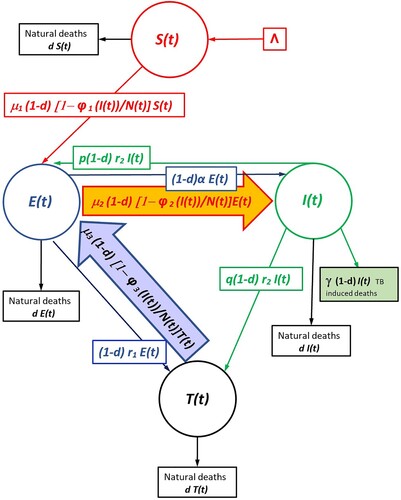
After one unit of time, a susceptible individual can be infected through contact with the infectious and enter the latent or exposed class, still be in the susceptible class, or die. A latent individual may become infectious and enter the infectious class, get tested and, subsequently, be treated, pass into the treated class, stay in the latent class, or die. An infected can be treated and enter the treated or recovered class, stay in the infectious class, or die. According to [17], an infected may also revert to exposed status. A treated individual can recover by effective treatment or regress back to the exposed class, stay in the treated/recovered class, or die. Many researchers have expounded that certain features of TB dynamics, such as slow transmission and complicated parameter estimation, require updated methods. The ambiguity of the SEIT model derives from people in the infectious compartment getting treatment. Some proportion q move to the recovered class, while a proportion p does not complete treatment and relapse to the latent class, which causes an influx of exposed individuals that may be interpreted as new infections. Consequently, we have two options: (1) view the relapse term $p{r}_{2}I$ as new infections or (2) view the relapse term as existing infections [4]. The data presented in [4] chronicles the re-emergence of tuberculosis during the 1980s, coinciding with the HIV/AIDS epidemic. TB rates began to rise from a low of 22,201 cases in 1985, accelerating in the early 1990s and peaking at 26,673 in 1992. Rates of latent TB have always been high among injecting drug users, and NIDA (National Institute on Drug Abuse) [27] studies demonstrate that HIV infection, which is also prevalent among intravenous drug users, can activate latent TB. Lack of access to TB therapy or failure to complete a full course of treatment due to costs additionally contributes to active TB development and transmission. A 2018 report by Ma et al. [4] states that TB incidence in San Francisco peaked between 1991 and 1993 because of the TB/HIV co-epidemic, which produced a high estimated reproductive number of around 2.1. As may be seen in the chart flow Figure 2, the SEIT model is given below. (31) $\begin{array}{rl}S(t+1)& =\mathrm{\Lambda }+(1-{\mu }_1)(1-d)S\left(t\right)+{\mu }_1(1-d){\phi }_1\left(I\right(t\left)/N\right(t\left)\right)S\left(t\right)\\ E(t+1)& ={\mu }_1(1-d)(1-{\phi }_1(I\left(t\right)/N\left(t\right)\left)S\right(t)+{\mu }_2(1-d\left){\phi }_2\right(I\left(t\right)/N\left(t\right)\left)E\right(t)\\ & +{\mu }_3(1-d)(1-{\phi }_3(I\left(t\right)/N\left(t\right)\left)T\right(t)+(1-d\left)\right(1-\alpha -r_1-{\mu }_2\left)E\right(t)\\ & +p(1-d)r_{2}I\left(t\right)\\ I(t+1)& =\alpha (1-d)E\left(t\right)+{\mu }_2(1-d)(1-{\phi }_2(I\left(t\right)/N\left(t\right)\left)E\right(t)+(1-d\left)\right(1-r_2-\gamma \left)I\right(t)\\ T(t+1)& =r_1(1-d)E\left(t\right)+q(1-d)r_{2}I\left(t\right)+{\mu }_3\left)\right(1-d\left){\phi }_3\right(I\left(t\right)/N\left(t\right)\left)T\right(t)\\ & +(1-{\mu }_3)(1-d)T\left(t\right)\end{array}$(31) where ${\phi }_i\left(I/N\right)=e^{-{\text{β}}_{i}I/N}$, i=1,2,3, and p + q = 1)

Figure 2. Chartflow of the exogenous model with treatment.

Assuming $\gamma =0$, then $N(t+1)=\mathrm{\Lambda }+(1-d)N\left(t\right)$ and thus the equilibrium $N\left(t\right)\to \mathrm{\Lambda }/d=N^{\ast }$ Hence, we may study the above system with $N\left(t\right)$ replaced by $N^{\ast }$ and we have the limiting equation (32) $\begin{array}{rl}S(t+1)& =\mathrm{\Lambda }+(1-{\mu }_1)(1-d)S\left(t\right)+{\mu }_1(1-d){\phi }_1\left(I\right(t\left)/N^{\ast }\right)S\left(t\right)\\ E(t+1)& ={\mu }_1(1-d)(1-{\phi }_1(I\left(t\right)/N^{\ast }\left)S\right(t)+{\mu }_2(1-d\left){\phi }_2\right(I\left(t\right)/N^{\ast }\left)E\right(t)\\ & +{\mu }_3(1-d)(1-{\phi }_3(I\left(t\right)/N^{\ast }\left)T\right(t)\\ & +(1-d)(1-\alpha -r_1-{\mu }_2)E\left(t\right)+p(1-d)r_{2}I\left(t\right)\\ I(t+1)& =\alpha (1-d)E\left(t\right)+{\mu }_2(1-d)(1-{\phi }_2(I\left(t\right)/N^{\ast }\left)E\right(t)+(1-d\left)\right(1-r_2\left)I\right(t)\\ T(t+1)& =r_1(1-d)E\left(t\right)+q(1-d)r_{2}I\left(t\right)+{\mu }_3(1-d){\phi }_3\left(I\right(t\left)/N^{\ast }\right)T\left(t\right)\\ & +(1-{\mu }_3)(1-d)T\left(t\right)\end{array}$(32)

7.1. The computation of ${\mathcal{R}}_0({\mathcal{E}}_0$)

We are going to use the next-generation matrix approach [15]. Let $X_0=(E,I{)}^T$, $X_1=(S,T{)}^T$, $X=(X_0,X_1)\in R_{+}^4$. Hence system (34(34) $\begin{array}{rl}S(t+1)& =\mathrm{\Lambda }+(1-{\mu }_1)(1-d)S\left(t\right)+{\mu }_1(1-d){\phi }_1\left(I\right(t\left)/N^{\ast }\right)S\left(t\right)\\ E(t+1)& ={\mu }_1(1-d)(1-{\phi }_1(I\left(t\right)/N^{\ast }\left)S\right(t)+{\mu }_3(1-d\left)\right(1-{\phi }_3\left(I\right(t\left)/N^{\ast }\right)T\left(t\right)\\ & +(1-d)(1-\alpha -r_1)E\left(t\right)+p(1-d)r_{2}I\left(t\right)\\ I(t+1)& =\alpha (1-d)E\left(t\right)+(1-d)(1-r_2)I\left(t\right)\\ T(t+1)& =r_1(1-d)E\left(t\right)+q(1-d)r_{2}I\left(t\right)+{\mu }_3(1-d){\phi }_3\left(I\right(t\left)/N^{\ast }\right)T\left(t\right)\\ & +(1-{\mu }_3)(1-d)T\left(t\right)\end{array}$(34) ) may be written as (33) $\begin{array}{rl}{X}_0(t+1)& =G_0\left(X\right(t\left)\right)\\ X_1(t+1)& =G_1\left(X\right(t\left)\right)\end{array}$(33) where $G_0\left(X\right(t\left)\right)=\left(\begin{array}{c}E(t+1)\\ I(t+1)\end{array}\right)=\mathcal{F}\left(t\right)+\mathcal{T}\left(t\right)$, and $G_1\left(X\right(t\left)\right)=\left(\begin{array}{c}S(t+1)\\ T(t+1)\end{array}\right)$, where $\begin{array}{rl}\mathcal{F}\left(t\right)& =\left(\begin{array}{c}{\mu }_1(1-d)(1-{\phi }_1(I\left(t\right)/N^{\ast }\left)S\right(t)+{\mu }_3(1-d\left)\right(1-{\phi }_3\left(I\right(t\left)/N^{\ast }\right)\left)T\right(t)+p{r}_{2}I(t)\\ {\mu }_2(1-{\phi }_2(I\left(t\right)/N^{\ast }\left)E\right(t)\end{array}\right)\\ & =\left(\begin{array}{c}{\mathcal{F}}_1\left(t\right)\\ {\mathcal{F}}_2\left(t\right)\end{array}\right)\end{array}$is the vector of new infections that survive in the time interval $[0,t]$, and $\mathcal{T}\left(t\right)=\left(\begin{array}{c}(1-d-\alpha -r_1)E\left(t\right)+{\mu }_2{\phi }_2\left(I\right(t\left)/N^{\ast }\right)E\left(t\right)\\ \mathrm{\alpha E}\left(t\right)+(1-d-r_2-\gamma )I\left(t\right)\end{array}\right)=\left(\begin{array}{c}{\mathcal{T}}_1\left(t\right)\\ {\mathcal{T}}_2\left(t\right)\end{array}\right)$is the vector of all other transitions.

Next, we compute the Jacobian matrix of $\mathcal{T}\left(t\right)$ and $\mathcal{F}\left(t\right)$ at the disease-free equilibrium (DFE) ${\mathcal{E}}_0=(0,0,0,S^{\ast })$ $\begin{array}{rl}F\left(t\right){|}_{(0,0,S^{\ast },0)}& =\left(\begin{array}{cc}{\displaystyle \frac{\mathrm{\partial }{\mathcal{F}}_1\left(t\right)}{\mathrm{\partial }E}}& {\displaystyle \frac{\mathrm{\partial }{\mathcal{F}}_1\left(t\right)}{\mathrm{\partial }I}}\\ {\displaystyle \frac{\mathrm{\partial }{\mathcal{F}}_2\left(t\right)}{\mathrm{\partial }E}}& {\displaystyle \frac{\mathrm{\partial }{\mathcal{F}}_2\left(t\right)}{\mathrm{\partial }E}}\end{array}\right)=\left(\begin{array}{cc}0& p{r}_2(1-d)+{\mu }_1(1-d){\text{β}}_1\\ 0& 0\end{array}\right)\\ T\left(t\right){|}_{(0,0,S^{\ast },0)}& =\left(\begin{array}{cc}{\displaystyle \frac{\mathrm{\partial }{\mathcal{T}}_1\left(t\right)}{\mathrm{\partial }E}}& {\displaystyle \frac{\mathrm{\partial }{\mathcal{T}}_1\left(t\right)}{\mathrm{\partial }I}}\\ {\displaystyle \frac{\mathrm{\partial }{\mathcal{T}}_2\left(t\right)}{\mathrm{\partial }E}}& {\displaystyle \frac{\mathrm{\partial }{\mathcal{T}}_2\left(t\right)}{\mathrm{\delta I}}}\end{array}\right)\\ & =\left(\begin{array}{cc}(1-d)(1-\alpha -r_1)-{\mu }_2(1-d)& 0\\ \alpha (1-d)& (1-d)(1-\gamma -r_2)\end{array}\right).\end{array}$Now the basic reproduction number is given by ${\mathcal{R}}_0=\rho \left(F\right(I-T{)}^{-1})$, where ρ denotes the spectral radius of a matrix [15–17].

Hence ${\mathcal{R}}_0=\frac{\alpha (1-d{)}^2({\mu }_1{\text{β}}_1+p{r}_2)}{(1-(1-d\left)\right(1-\alpha -r_1)-{\mu }_2(1-d\left)\right)(1-(1-d\left)\right(1-\gamma -r_2\left)\right)}$. The expression gives the number of secondary infections that one infected will produce in an entirely susceptible population during its lifespan.

The statement in blue below needs to be revised

As it happens, ${\text{β}}_{1}S+{\text{β}}_{2}T$ is the number of secondary infections that one infected individual will produce in a unit of time. If the population is entirely susceptible, then T = 0. The lifespan of an infectious individual is $1/(d+\gamma +r_2)$. However, only a fraction $\alpha /(d+\alpha +r_1)$ survives the exposed period and moves to infected status. The fraction $\left(\mathrm{\alpha p}{r}_2\right)/(d+\alpha +r_1)(d+\gamma +r_2)$ gives the infected individuals who relapse, survive the exposed period, and become infectious again.

7.2. Local stability of DFE of the SEIT model

Theorem 7.1

The DFE $\left({\mathcal{E}}_0\right)$ of system (31(31) $\begin{array}{rl}S(t+1)& =\mathrm{\Lambda }+(1-{\mu }_1)(1-d)S\left(t\right)+{\mu }_1(1-d){\phi }_1\left(I\right(t\left)/N\right(t\left)\right)S\left(t\right)\\ E(t+1)& ={\mu }_1(1-d)(1-{\phi }_1(I\left(t\right)/N\left(t\right)\left)S\right(t)+{\mu }_2(1-d\left){\phi }_2\right(I\left(t\right)/N\left(t\right)\left)E\right(t)\\ & +{\mu }_3(1-d)(1-{\phi }_3(I\left(t\right)/N\left(t\right)\left)T\right(t)+(1-d\left)\right(1-\alpha -r_1-{\mu }_2\left)E\right(t)\\ & +p(1-d)r_{2}I\left(t\right)\\ I(t+1)& =\alpha (1-d)E\left(t\right)+{\mu }_2(1-d)(1-{\phi }_2(I\left(t\right)/N\left(t\right)\left)E\right(t)+(1-d\left)\right(1-r_2-\gamma \left)I\right(t)\\ T(t+1)& =r_1(1-d)E\left(t\right)+q(1-d)r_{2}I\left(t\right)+{\mu }_3\left)\right(1-d\left){\phi }_3\right(I\left(t\right)/N\left(t\right)\left)T\right(t)\\ & +(1-{\mu }_3)(1-d)T\left(t\right)\end{array}$(31) ) is locally asymptotically stable if ${\mathcal{R}}_0\left({\mathcal{E}}_0\right)<1$ and unstable if ${\mathcal{R}}_0\left({\mathcal{E}}_0\right)>1$.

Proof.

The Jacobian matrix of system (34(34) $\begin{array}{rl}S(t+1)& =\mathrm{\Lambda }+(1-{\mu }_1)(1-d)S\left(t\right)+{\mu }_1(1-d){\phi }_1\left(I\right(t\left)/N^{\ast }\right)S\left(t\right)\\ E(t+1)& ={\mu }_1(1-d)(1-{\phi }_1(I\left(t\right)/N^{\ast }\left)S\right(t)+{\mu }_3(1-d\left)\right(1-{\phi }_3\left(I\right(t\left)/N^{\ast }\right)T\left(t\right)\\ & +(1-d)(1-\alpha -r_1)E\left(t\right)+p(1-d)r_{2}I\left(t\right)\\ I(t+1)& =\alpha (1-d)E\left(t\right)+(1-d)(1-r_2)I\left(t\right)\\ T(t+1)& =r_1(1-d)E\left(t\right)+q(1-d)r_{2}I\left(t\right)+{\mu }_3(1-d){\phi }_3\left(I\right(t\left)/N^{\ast }\right)T\left(t\right)\\ & +(1-{\mu }_3)(1-d)T\left(t\right)\end{array}$(34) ) at ${\mathcal{E}}_0$ represented by $J\left({\mathcal{E}}_0\right)$ is given by $J\left({\mathcal{E}}_0\right)=\left(\begin{array}{cccc}-d+1& 0& -{\mu }_1{\text{β}}_1& 0\\ 0& 1-d-\alpha -r_1-{\mu }_2& p{r}_2+{\mu }_1{\text{β}}_1& 0\\ 0& \alpha & 1-d-\gamma -r_2& 0\\ 0& r_1& q{r}_2& 1-d\end{array}\right)$The first eigenvalue of the Jacobian matrix is ${\lambda }_1={\lambda }_4=1-d<1$. The remaining two eigenvalues are the eigenvalues of the matrix $A=\left(\begin{array}{cc}1-d-\alpha -r_1-{\mu }_2& p{r}_2+{\mu }_1{\text{β}}_1\\ \alpha & 1-d-\gamma -r_2\end{array}\right),$We now use the determinant-trace criteria to show that the two eigenvalues of this matrix lie inside the unit disk [18,19]. One may show that the eigenvalues of A are inside the unit disk if ${\mathcal{R}}_0<1$ and unstable if ${\mathcal{R}}_0>1$ Now if ${\mathcal{R}}_0=1$, then $\det \left(A\right)=\mathrm{tr}\left(A\right)-1$. This implies that ${\lambda }_2=1$ and $|{\lambda }_3|<1$ and the system goes through transcritcal bifurcation.

Next, we state the global stability result of DFE.

Theorem 7.2

Assume that ${\mathcal{R}}_0\le 1$. Then the DFE of (31(31) $\begin{array}{rl}S(t+1)& =\mathrm{\Lambda }+(1-{\mu }_1)(1-d)S\left(t\right)+{\mu }_1(1-d){\phi }_1\left(I\right(t\left)/N\right(t\left)\right)S\left(t\right)\\ E(t+1)& ={\mu }_1(1-d)(1-{\phi }_1(I\left(t\right)/N\left(t\right)\left)S\right(t)+{\mu }_2(1-d\left){\phi }_2\right(I\left(t\right)/N\left(t\right)\left)E\right(t)\\ & +{\mu }_3(1-d)(1-{\phi }_3(I\left(t\right)/N\left(t\right)\left)T\right(t)+(1-d\left)\right(1-\alpha -r_1-{\mu }_2\left)E\right(t)\\ & +p(1-d)r_{2}I\left(t\right)\\ I(t+1)& =\alpha (1-d)E\left(t\right)+{\mu }_2(1-d)(1-{\phi }_2(I\left(t\right)/N\left(t\right)\left)E\right(t)+(1-d\left)\right(1-r_2-\gamma \left)I\right(t)\\ T(t+1)& =r_1(1-d)E\left(t\right)+q(1-d)r_{2}I\left(t\right)+{\mu }_3\left)\right(1-d\left){\phi }_3\right(I\left(t\right)/N\left(t\right)\left)T\right(t)\\ & +(1-{\mu }_3)(1-d)T\left(t\right)\end{array}$(31) ) is globally asymptotically stable.

Proof.

The proof is similar to the proof of Theorem 3.1 and will be omitted

7.3. Reproduction number computed using the endemic equilibrium

Assuming $\gamma =0$, then $N(t+1)=\mathrm{\Lambda }+(1-d)N\left(t\right)$ and thus the equilibrium $N\left(t\right)\to \mathrm{\Lambda }/d=N^{\ast }$. We also assume that ${\mu }_2=0$. Hence, we may study the above system with $N\left(t\right)$ replaced by $N^{\ast }$ and we have the limiting equation (34) $\begin{array}{rl}S(t+1)& =\mathrm{\Lambda }+(1-{\mu }_1)(1-d)S\left(t\right)+{\mu }_1(1-d){\phi }_1\left(I\right(t\left)/N^{\ast }\right)S\left(t\right)\\ E(t+1)& ={\mu }_1(1-d)(1-{\phi }_1(I\left(t\right)/N^{\ast }\left)S\right(t)+{\mu }_3(1-d\left)\right(1-{\phi }_3\left(I\right(t\left)/N^{\ast }\right)T\left(t\right)\\ & +(1-d)(1-\alpha -r_1)E\left(t\right)+p(1-d)r_{2}I\left(t\right)\\ I(t+1)& =\alpha (1-d)E\left(t\right)+(1-d)(1-r_2)I\left(t\right)\\ T(t+1)& =r_1(1-d)E\left(t\right)+q(1-d)r_{2}I\left(t\right)+{\mu }_3(1-d){\phi }_3\left(I\right(t\left)/N^{\ast }\right)T\left(t\right)\\ & +(1-{\mu }_3)(1-d)T\left(t\right)\end{array}$(34) Let $X_0=(E,I{)}^T$, $X_1=(S,T{)}^T$, $X=(X_0,X_1)\in R_{+}^4$. Hence system (34(34) $\begin{array}{rl}S(t+1)& =\mathrm{\Lambda }+(1-{\mu }_1)(1-d)S\left(t\right)+{\mu }_1(1-d){\phi }_1\left(I\right(t\left)/N^{\ast }\right)S\left(t\right)\\ E(t+1)& ={\mu }_1(1-d)(1-{\phi }_1(I\left(t\right)/N^{\ast }\left)S\right(t)+{\mu }_3(1-d\left)\right(1-{\phi }_3\left(I\right(t\left)/N^{\ast }\right)T\left(t\right)\\ & +(1-d)(1-\alpha -r_1)E\left(t\right)+p(1-d)r_{2}I\left(t\right)\\ I(t+1)& =\alpha (1-d)E\left(t\right)+(1-d)(1-r_2)I\left(t\right)\\ T(t+1)& =r_1(1-d)E\left(t\right)+q(1-d)r_{2}I\left(t\right)+{\mu }_3(1-d){\phi }_3\left(I\right(t\left)/N^{\ast }\right)T\left(t\right)\\ & +(1-{\mu }_3)(1-d)T\left(t\right)\end{array}$(34) ) may be written as (35) $\begin{array}{rl}{X}_0(t+1)& =G_0\left(X\right(t\left)\right)\\ X_1(t+1)& =G_1\left(X\right(t\left)\right)\end{array}$(35) where $G_0\left(X\right(t\left)\right)=\left(\begin{array}{c}E(t+1)\\ I(t+1)\end{array}\right)=\mathcal{F}\left(t\right)+\mathcal{T}\left(t\right)$, and $G_1\left(X\right(t\left)\right)=\left(\begin{array}{c}S(t+1)\\ T(t+1)\end{array}\right)$, where $\begin{array}{rl}\mathcal{F}\left(t\right)& =\left(\begin{array}{l}{\mu }_1(1-d)(1-{\phi }_1(I\left(t\right)/N^{\ast }\left)S\right(t)+{\mu }_3((1-d)1-{\phi }_3\left(I\right(t\left)/N^{\ast }\right)T\left(t\right)\\ +p{r}_2(1-d)I\left(t\right)\\ 0\end{array}\right)\\ & =\left(\begin{array}{c}{\mathcal{F}}_1\left(t\right)\\ {\mathcal{F}}_2\left(t\right)\end{array}\right)\end{array}$is the vector of new infections that survive in the time interval $[0,t]$, and $\mathcal{T}\left(t\right)=\left(\begin{array}{c}(1-d)(1-\alpha -r_1)E\left(t\right)\\ \alpha (1-d)E\left(t\right)+(1-d)(1-r_2)I\left(t\right)\end{array}\right)=\left(\begin{array}{c}{\mathcal{T}}_1\left(t\right)\\ {\mathcal{T}}_2\left(t\right)\end{array}\right)$is the vector of all other transitions.

Next, we compute the Jacobian matrix of $\mathcal{T}\left(t\right)$ and $\mathcal{F}\left(t\right)$ at the endemic equilibrium (EE) ${\mathcal{E}}_0=(E^{\ast },I^{\ast },S^{\ast },T^{\ast })$ $\begin{array}{rl}F\left(t\right){|}_{(E^{\ast },I^{\ast },S^{\ast },T^{\ast })}& =\left(\begin{array}{cc}{\displaystyle \frac{\mathrm{\partial }{\mathcal{F}}_1\left(t\right)}{\mathrm{\partial }E}}& \frac{\mathrm{\partial }{\mathcal{F}}_1\left(t\right)}{\mathrm{\partial }I}\\ {\displaystyle \frac{\mathrm{\partial }{\mathcal{F}}_2\left(t\right)}{\mathrm{\partial }E}}& {\displaystyle \frac{\mathrm{\partial }{\mathcal{F}}_2\left(t\right)}{\mathrm{\partial }E}}\end{array}\right)\\ & =\left(\begin{array}{cc}0& (1-d)(p{r}_2+{\mu }_1{\text{β}}_1{\phi }_1(I^{\ast }/N^{\ast })S^{\ast }/N^{\ast }+{\mu }_3{\text{β}}_1{\phi }_3(I^{\ast }/N^{\ast }\left)T^{\ast }/N^{\ast }\right)\\ 0& 0\end{array}\right)\\ T\left(t\right){|}_{(E^{\ast },I^{\ast },S^{\ast },T^{\ast })}& =\left(\begin{array}{cc}{\displaystyle \frac{\mathrm{\partial }{\mathcal{T}}_1\left(t\right)}{\mathrm{\partial }E}}& {\displaystyle \frac{\mathrm{\partial }{\mathcal{T}}_1\left(t\right)}{\mathrm{\partial }I}}\\ {\displaystyle \frac{\mathrm{\partial }{\mathcal{T}}_2\left(t\right)}{\mathrm{\partial }E}}& {\displaystyle \frac{\mathrm{\partial }{\mathcal{T}}_2\left(t\right)}{\mathrm{\delta I}}}\end{array}\right)\\ & =\left(\begin{array}{cc}(1-d)(1-\alpha -r_1-{\mu }_2)& 0\\ \alpha (1-d)& (1-d)(1-r_2)\end{array}\right).\end{array}$Now the basic reproduction number is given by ${\mathcal{R}}_0\left({\mathcal{E}}^{\ast }\right)=\rho \left(F\right(I-T\left){)}^{-1}\right)$, where ρ denotes the spectral radius of a matrix [15–17]. Hence ${\mathcal{R}}_0\left({\mathcal{E}}^{\ast }\right)=\frac{\alpha (1-d{)}^2(p{r}_2+{\mu }_1{\text{β}}_1{\phi }_1\left(I^{\ast }/N^{\ast }\right)S^{\ast }/N^{\ast }+{\mu }_3{\text{β}}_1{\phi }_3\left(I^{\ast }/N^{\ast }\right)T^{\ast }/N^{\ast }\left)\right)}{(d+\alpha +r_1+{\mu }_2)(d+r_2+\gamma )+\alpha {\mu }_2{\text{β}}_2{\phi }_2\left(I^{\ast }/N^{\ast }\right)T^{\ast }/N^{\ast }}$. The expression gives the number of secondary infections that one infected will produce in an entirely susceptible population during its lifespan. This expression reduces to the net reproduction number based on the disease-free equilibrium.

8. Existence of the endemic equilibrium of the SEIT compartmental model (with treatment)

8.1. case $\gamma \ne 0$, ${\mu }_1\ne 0$, $r_1\ne 0$, $r_2\ne 0$, ${\mu }_2=0$, ${\mu }_3=0$

Proposition 8.1

Assume that $\gamma \ne 0$, ${\mu }_1\ne 0$, $r_1\ne 0$, $r_2\ne 0$, ${\mu }_2=0$ and ${\mu }_3=0$. Then every equilibrium point ${\mathcal{E}}^{\ast }=(S^{\ast },E^{\ast },I^{\ast },T^{\ast }$) of model (34(34) $\begin{array}{rl}S(t+1)& =\mathrm{\Lambda }+(1-{\mu }_1)(1-d)S\left(t\right)+{\mu }_1(1-d){\phi }_1\left(I\right(t\left)/N^{\ast }\right)S\left(t\right)\\ E(t+1)& ={\mu }_1(1-d)(1-{\phi }_1(I\left(t\right)/N^{\ast }\left)S\right(t)+{\mu }_3(1-d\left)\right(1-{\phi }_3\left(I\right(t\left)/N^{\ast }\right)T\left(t\right)\\ & +(1-d)(1-\alpha -r_1)E\left(t\right)+p(1-d)r_{2}I\left(t\right)\\ I(t+1)& =\alpha (1-d)E\left(t\right)+(1-d)(1-r_2)I\left(t\right)\\ T(t+1)& =r_1(1-d)E\left(t\right)+q(1-d)r_{2}I\left(t\right)+{\mu }_3(1-d){\phi }_3\left(I\right(t\left)/N^{\ast }\right)T\left(t\right)\\ & +(1-{\mu }_3)(1-d)T\left(t\right)\end{array}$(34) ) is of the form (36) ${\mathcal{E}}^{\ast }=(S^{\ast },\frac{(d+r_2-d{r}_2)(\mathrm{\Lambda }-d{S}^{\ast })}{L_1},\frac{\alpha (1-d)(\mathrm{\Lambda }-d{S}^{\ast })}{L_1},\frac{L_2(\mathrm{\Lambda }-d{S}^{\ast })}{L_1})$(36) with $S^{\ast }$ solution of (37) $L_1{N}^{\ast }\ln \left[\frac{{\mu }_1(1-d)S^{\ast }}{({\mu }_1+d-{\mu }_{1}d)S^{\ast }-\mathrm{\Lambda }}\right]+\alpha {\text{β}}_1(1-d)\mathrm{d}{S}^{\ast }=(1-d)\alpha {\text{β}}_1\mathrm{\Lambda },$(37) with $L_1=[\left[\right(1-d\left)\right(\alpha +r_1)+d](d+r_2-d{r}_2)-\alpha (1-d{)}^{2}p{r}_2],$ and $L_2=\left[r_1\right(d+r_2-d{r}_2)+(1-d\left)q{r}_2\alpha \right]$.

This equation can also be written as (38) $L_1{N}^{\ast }[\ln (S^{\ast })-\ln \left[\right({\mu }_1+d)S^{\ast }-\mathrm{\Lambda }]]+\alpha {\text{β}}_1\mathrm{d}{S}^{\ast }=\alpha {\text{β}}_1\mathrm{\Lambda }-L_1{N}^{\ast }\ln \left({\mu }_1\right),$(38)

Proof.

Consider $S(t+1)=\mathrm{\Lambda }+(1-{\mu }_1)(1-d)S\left(t\right)+{\mu }_1(1-d){\mathrm{e}}^{-{\text{β}}_1\left(I\right(t\left)/N^{\ast }\right)}S\left(t\right)$when $S(t+1)=S\left(t\right)$,

one has: (39) $(1-d){\mu }_1{\mathrm{e}}^{-{\text{β}}_1\frac{I^{\ast }}{N^{\ast }}}{S}^{\ast }=-\mathrm{\Lambda }+({\mu }_1+d-{\mu }_{1}d)S^{\ast }$(39) then if ${\mu }_1>0$, ${\text{β}}_1>0$ and $S^{\ast }>0$ ${\mathrm{e}}^{-{\text{β}}_1\frac{I^{\ast }}{N^{\ast }}}=\frac{-\mathrm{\Lambda }+({\mu }_1+d-{\mu }_{1}d)S^{\ast }}{(1-d){\mu }_1{S}^{\ast }}$or (40) $\begin{array}{rl}& \ln \left[{\mathrm{e}}^{-{\text{β}}_1\frac{I^{\ast }}{N^{\ast }}}\right]=\ln \left[\frac{-\mathrm{\Lambda }+({\mu }_1+d-{\mu }_{1}d)S^{\ast }}{(1-d){\mu }_1{S}^{\ast }}\right]\\ & -{\text{β}}_1\frac{I^{\ast }}{N^{\ast }}=\ln \left[\frac{-\mathrm{\Lambda }+({\mu }_1+d-{\mu }_{1}d)S^{\ast }}{(1-d){\mu }_1{S}^{\ast }}\right]\\ & I^{\ast }=-\frac{N^{\ast }}{{\text{β}}_1}\ln \left[\frac{-\mathrm{\Lambda }+({\mu }_1+d-{\mu }_{1}d)S^{\ast }}{(1-d){\mu }_1{S}^{\ast }}\right]\end{array}$(40) Consider now $E(t+1)=(1-d){\mu }_1(1-{\mathrm{e}}^{-{\text{β}}_1\left(I\right(t\left)/N^{\ast }\right)})S\left(t\right)+(1-d)(1-\alpha -r_1)E\left(t\right)+(1-d)p{r}_{2}I\left(t\right)$when $E(t+1)=E\left(t\right)$, one has: $0={\mu }_1(1-d)(1-{\mathrm{e}}^{-{\text{β}}_1\frac{I^{\ast }}{N^{\ast }}})S^{\ast }-\left[\right(1-d\left)\right(\alpha +r_1)+d]E^{\ast }+(1-d)p{r}_{2}I\left(t\right)$From (39(39) $(1-d){\mu }_1{\mathrm{e}}^{-{\text{β}}_1\frac{I^{\ast }}{N^{\ast }}}{S}^{\ast }=-\mathrm{\Lambda }+({\mu }_1+d-{\mu }_{1}d)S^{\ast }$(39) ) it comes: (41) $\begin{array}{rl}& 0={\mu }_1(1-d)S^{\ast }+\mathrm{\Lambda }-({\mu }_1+d{\mu }_{1}d)-S^{\ast }-\left[\right(1-d\left)\right(\alpha +r_1)+d]E^{\ast }+(1-d)p{r}_{2}I\left(t\right)\\ & \left[\right(1-d\left)\right(\alpha +r_1)+d]E^{\ast }+(1-d)p{r}_{2}I\left(t\right)=\mathrm{\Lambda }-d{S}^{\ast }\end{array}$(41) Consider now $I(t+1)=\alpha (1-d)E\left(t\right)+(1-d)(1-r_2)I\left(t\right)$when $I(t+1)=I\left(t\right)$, one has: (42) $\begin{array}{rl}& 0=\alpha (1-d)E^{\ast }-(d+r_2-d{r}_2)I^{\ast }\\ & E^{\ast }=\frac{(d+r_2-d{r}_2){\mathcal{I}}^{\mathcal{\ast }}}{\alpha (1-d)}\end{array}$(42) inserting (42(42) $\begin{array}{rl}& 0=\alpha (1-d)E^{\ast }-(d+r_2-d{r}_2)I^{\ast }\\ & E^{\ast }=\frac{(d+r_2-d{r}_2){\mathcal{I}}^{\mathcal{\ast }}}{\alpha (1-d)}\end{array}$(42) ) in (41(41) $\begin{array}{rl}& 0={\mu }_1(1-d)S^{\ast }+\mathrm{\Lambda }-({\mu }_1+d{\mu }_{1}d)-S^{\ast }-\left[\right(1-d\left)\right(\alpha +r_1)+d]E^{\ast }+(1-d)p{r}_{2}I\left(t\right)\\ & \left[\right(1-d\left)\right(\alpha +r_1)+d]E^{\ast }+(1-d)p{r}_{2}I\left(t\right)=\mathrm{\Lambda }-d{S}^{\ast }\end{array}$(41) ) we obtain: (43) $\frac{\left[\right(1-d\left)\right(\alpha +r_1)+d](d+r_2-d{r}_2){\mathcal{I}}^{\mathcal{\ast }}}{(1-d)\alpha }-(1-d)p{r}_2{\mathcal{I}}^{\mathcal{\ast }}=\mathrm{\Lambda }-d{S}^{\ast }$(43) or (44) $\frac{[\left[\right(1-d\left)\right(\alpha +r_1)+d](d+r_2-d{r}_2)-\alpha (1-d{)}^{2}p{r}_2]{\mathcal{I}}^{\mathcal{\ast }}}{(1-d)\alpha }=\mathrm{\Lambda }-d{S}^{\ast }$(44) thus, as $L_1=\left[\left[\right(1-d\left)\right(\alpha +r_1)+d]\right(d+r_2-d{r}_2)-\alpha (1-d{)}^{2}p{r}_2]$ (45) ${\mathcal{I}}^{\mathcal{\ast }}=\frac{\alpha (1-d)(\mathrm{\Lambda }-d{S}^{\ast })}{L_1}$(45) Equaling (40(40) $\begin{array}{rl}& \ln \left[{\mathrm{e}}^{-{\text{β}}_1\frac{I^{\ast }}{N^{\ast }}}\right]=\ln \left[\frac{-\mathrm{\Lambda }+({\mu }_1+d-{\mu }_{1}d)S^{\ast }}{(1-d){\mu }_1{S}^{\ast }}\right]\\ & -{\text{β}}_1\frac{I^{\ast }}{N^{\ast }}=\ln \left[\frac{-\mathrm{\Lambda }+({\mu }_1+d-{\mu }_{1}d)S^{\ast }}{(1-d){\mu }_1{S}^{\ast }}\right]\\ & I^{\ast }=-\frac{N^{\ast }}{{\text{β}}_1}\ln \left[\frac{-\mathrm{\Lambda }+({\mu }_1+d-{\mu }_{1}d)S^{\ast }}{(1-d){\mu }_1{S}^{\ast }}\right]\end{array}$(40) ) to (45(45) ${\mathcal{I}}^{\mathcal{\ast }}=\frac{\alpha (1-d)(\mathrm{\Lambda }-d{S}^{\ast })}{L_1}$(45) ) it comes (46) $\frac{\alpha \left(\right(\mathrm{\Lambda }-d{S}^{\ast })}{L_1}=-\frac{N^{\ast }}{{\text{β}}_1}\ln \left[\frac{-\mathrm{\Lambda }+({\mu }_1+d-{\mu }_{1}d)S^{\ast }}{(1-d){\mu }_1{S}^{\ast }}\right]-d)$(46) or (47) $L_1{N}^{\ast }\ln \left[\frac{(1-d){\mu }_1{S}^{\ast }}{({\mu }_1+d-{\mu }_{1}d)S^{\ast }-\mathrm{\Lambda }}\right]+(1-d)\alpha {\text{β}}_{1}d{S}^{\ast }=(1-d)\alpha {\text{β}}_1\mathrm{\Lambda }$(47) Considering now the fourth equation of (34(34) $\begin{array}{rl}S(t+1)& =\mathrm{\Lambda }+(1-{\mu }_1)(1-d)S\left(t\right)+{\mu }_1(1-d){\phi }_1\left(I\right(t\left)/N^{\ast }\right)S\left(t\right)\\ E(t+1)& ={\mu }_1(1-d)(1-{\phi }_1(I\left(t\right)/N^{\ast }\left)S\right(t)+{\mu }_3(1-d\left)\right(1-{\phi }_3\left(I\right(t\left)/N^{\ast }\right)T\left(t\right)\\ & +(1-d)(1-\alpha -r_1)E\left(t\right)+p(1-d)r_{2}I\left(t\right)\\ I(t+1)& =\alpha (1-d)E\left(t\right)+(1-d)(1-r_2)I\left(t\right)\\ T(t+1)& =r_1(1-d)E\left(t\right)+q(1-d)r_{2}I\left(t\right)+{\mu }_3(1-d){\phi }_3\left(I\right(t\left)/N^{\ast }\right)T\left(t\right)\\ & +(1-{\mu }_3)(1-d)T\left(t\right)\end{array}$(34) ) (48) $T(t+1)=(1-d)r_{1}E\left(t\right)+(1-d)q{r}_{2}I\left(t\right)+(1-d)T\left(t\right)$(48) when $T(t+1)=T\left(t\right)$,

It comes (49) ${\mathcal{T}}^{\ast }=\frac{(1-d)(r_1{E}^{\ast }+q{r}_2{I}^{\ast })}{d}$(49) or (50) ${\mathcal{T}}^{\ast }=\frac{\left[r_1\right(d+r_2-d{r}_2)+(1-d\left)q{r}_2\alpha \right]{\mathcal{I}}^{\mathcal{\ast }}}{d(1-d)\alpha }$(50) or (51) ${\mathcal{T}}^{\ast }=\frac{\left[r_1\right(d+r_2-d{r}_2)+(1-d\left)q{r}_2\alpha \right](\mathrm{\Lambda }-d{S}^{\ast })}{L_1}$(51) or, as $L_2=\left[r_1\right(d+r_2-d{r}_2)+(1-d\left)q{r}_2\alpha \right]$ (52) ${\mathcal{T}}^{\ast }=\frac{L_2(\mathrm{\Lambda }-d{S}^{\ast })}{L_1}$(52)

8.2. Existence and uniqueness of the endemic equilibrium

Theorem 8.2

Assume that $\gamma \ne 0$, ${\mu }_1\ne 0$, $r_1\ne 0$, $r_2\ne 0$, ${\mu }_2=0$, ${\mu }_3=0$ and ${\mathcal{R}}_0>1$. Then there exists a unique endemic equilibrium point ${\mathcal{E}}^{\ast }=(S^{\ast }>0$, $E^{\ast }\ge 0$, $I^{\ast }\ge 0$, ${\mathcal{T}}^{\ast }\ge 0$) of system (34(34) $\begin{array}{rl}S(t+1)& =\mathrm{\Lambda }+(1-{\mu }_1)(1-d)S\left(t\right)+{\mu }_1(1-d){\phi }_1\left(I\right(t\left)/N^{\ast }\right)S\left(t\right)\\ E(t+1)& ={\mu }_1(1-d)(1-{\phi }_1(I\left(t\right)/N^{\ast }\left)S\right(t)+{\mu }_3(1-d\left)\right(1-{\phi }_3\left(I\right(t\left)/N^{\ast }\right)T\left(t\right)\\ & +(1-d)(1-\alpha -r_1)E\left(t\right)+p(1-d)r_{2}I\left(t\right)\\ I(t+1)& =\alpha (1-d)E\left(t\right)+(1-d)(1-r_2)I\left(t\right)\\ T(t+1)& =r_1(1-d)E\left(t\right)+q(1-d)r_{2}I\left(t\right)+{\mu }_3(1-d){\phi }_3\left(I\right(t\left)/N^{\ast }\right)T\left(t\right)\\ & +(1-{\mu }_3)(1-d)T\left(t\right)\end{array}$(34) )

Proof.

Consider the function (53) $f\left(x\right)=L_1{N}^{\ast }\ln \left[\frac{(1-d){\mu }_{1}x}{({\mu }_1+d-{\mu }_{1}d)x-\mathrm{\Lambda }}\right]+(1-d)\alpha {\text{β}}_1\mathrm{dx},$(53) which is only defined for $x>\frac{\mathrm{\Lambda }}{{\mu }_1+d}$.

Its derivative is: (54) $f^{\mathrm{\prime }}\left(x\right)=-\frac{L_{1}N\mathrm{\Lambda }}{x\left[\right({\mu }_1+d-{\mu }_{1}d)x-\mathrm{\Lambda }]}+(1-d)\alpha {\text{β}}_{1}d,$(54) and its second derivative is: (55) $f^{\mathrm{\prime \prime }}\left(x\right)=\frac{L_{1}N\mathrm{\Lambda }\left[2\right({\mu }_1+d-{\mu }_{1}d)x-\mathrm{\Lambda }]}{x^2{\left[\right({\mu }_1+d-{\mu }_{1}d)x-\mathrm{\Lambda }]}^2},$(55) which is always positive because from (11(11) $\begin{array}{rl}& d(d+\alpha -\mathrm{\alpha d})N^{\ast }[(1-d)\ln \left(S^{\ast }\right)-\ln \left[\right({\mu }_1+d-{\mu }_{1}d)S^{\ast }-\mathrm{\Lambda }]]+(1-d)\alpha {\text{β}}_{1}d{S}^{\ast }\\ & =(1-d)\alpha {\text{β}}_1\mathrm{\Lambda }-d(d+\alpha +\mathrm{\alpha d})N^{\ast }\ln \left(\right(1-d\left){\mu }_1\right),\end{array}$(11) ) $({\mu }_1+d-{\mu }_{1}d)S^{\ast }-\mathrm{\Lambda }>0$, i.e. $({\mu }_1+d-{\mu }_{1}d)x-\mathrm{\Lambda }>0$,

hence $\mathrm{\Lambda }<({\mu }_1+d-{\mu }_{1}d)x<2({\mu }_1+d-{\mu }_{1}d)x$ and $L_1>0$ because $L_1=\left[\left[\right(1-d\left)\right(\alpha +r_1)+d]\right(d+r_2-d{r}_2)-\alpha (1-d{)}^{2}p{r}_2]$ it is known that $0<r_2<1$, the other parameters being positive, $L_1$ must be $>0$.

Therefore $f\left(x\right)$ is convex and $f^{\mathrm{\prime }}\left(x\right)$ is always increasing.

The equation (56) $f\left(x\right)=(1-d)\alpha {\text{β}}_1\mathrm{\Lambda },$(56) which represents the intersection of a convex curve with and horizontal straight line, and can have either zero, one, or two solutions.

Clearly, $x=N^{\ast }$ satisfies Equation (56(56) $f\left(x\right)=(1-d)\alpha {\text{β}}_1\mathrm{\Lambda },$(56) ), which gives us the disease equilibrium point $(S^{\ast },0,0,0)$. Therefore this equation can have only one or two solutions. Moreover, if ${\mathcal{R}}_0=1$, and since $N^{\ast }=\mathrm{\Lambda }/d$, it follows that (57) $f^{\mathrm{\prime }}\left(N^{\ast }\right)=-\frac{(d+\gamma )(d+\alpha )d\mathrm{\Lambda }}{{\mu }_1\mathrm{\Lambda }}+d\frac{(d+\gamma )(d+\alpha )}{{\mu }_1}=0,$(57) Therefore the tangent to the convex curve is horizontal, and, consequently, there is only one point of intersection between the horizontal line and the curve which is the DFE.

It is easy to verify that if ${\mathcal{R}}_0>1$ or $\alpha {\text{β}}_1>\frac{d(d+\alpha )}{\mu }$, then 1 $f^{\mathrm{\prime }}\left(N^{\ast }\right)>0$ and, consequently, there is an equilibrium point on the left-hand side intersection between the convex curve and the horizontal straight line, with $S^{\ast }<N^{\ast }$. This proves the existence and uniqueness of the endemic equilibrium point if ${\mathcal{R}}_0>1$.

9. Local stability of the endemic equilibrium of the SEIT compartmental model (with treatment)

Assume that ${\mu }_2=r_1=r_2=\gamma =0$. This implies that $\underset{t\to \mathrm{\infty }}{lim}T\left(t\right)=\underset{t\to \mathrm{\infty }}{lim}\left({\phi }_3\right(I\left(t\right)/N^{\ast })+1-{\mu }_3-d{)}^{t}T(0)=0$ In this case, the system (34(34) $\begin{array}{rl}S(t+1)& =\mathrm{\Lambda }+(1-{\mu }_1)(1-d)S\left(t\right)+{\mu }_1(1-d){\phi }_1\left(I\right(t\left)/N^{\ast }\right)S\left(t\right)\\ E(t+1)& ={\mu }_1(1-d)(1-{\phi }_1(I\left(t\right)/N^{\ast }\left)S\right(t)+{\mu }_3(1-d\left)\right(1-{\phi }_3\left(I\right(t\left)/N^{\ast }\right)T\left(t\right)\\ & +(1-d)(1-\alpha -r_1)E\left(t\right)+p(1-d)r_{2}I\left(t\right)\\ I(t+1)& =\alpha (1-d)E\left(t\right)+(1-d)(1-r_2)I\left(t\right)\\ T(t+1)& =r_1(1-d)E\left(t\right)+q(1-d)r_{2}I\left(t\right)+{\mu }_3(1-d){\phi }_3\left(I\right(t\left)/N^{\ast }\right)T\left(t\right)\\ & +(1-{\mu }_3)(1-d)T\left(t\right)\end{array}$(34) ) is equivalent to the SEI model (58) $\begin{array}{rl}S(t+1)& =\mathrm{\Lambda }+(1-{\mu }_1-d)S\left(t\right)+{\mu }_1{\phi }_1\left(I\right(t\left)/N^{\ast }\right)S\left(t\right)\\ E(t+1)& ={\mu }_1(1-{\phi }_1(I\left(t\right)/N^{\ast }\left)S\right(t)+(1-d-\alpha \left)E\right(t)\\ I(t+1)& =\mathrm{\alpha E}\left(t\right)+(1-d)I\left(t\right)\end{array}$(58)

Theorem 9.1

Assume that ${\mu }_2={\mu }_3=r_1=r_2=0$. and ${\mathcal{R}}_0\left({\mathcal{E}}^{\ast }\right)<1<{\mathcal{R}}_0\left({\mathcal{E}}_0\right)$. Then for sufficiently small $r_1$, $r_2$, and ${\mu }_2$, the endemic equilibrium of the system (34(34) $\begin{array}{rl}S(t+1)& =\mathrm{\Lambda }+(1-{\mu }_1)(1-d)S\left(t\right)+{\mu }_1(1-d){\phi }_1\left(I\right(t\left)/N^{\ast }\right)S\left(t\right)\\ E(t+1)& ={\mu }_1(1-d)(1-{\phi }_1(I\left(t\right)/N^{\ast }\left)S\right(t)+{\mu }_3(1-d\left)\right(1-{\phi }_3\left(I\right(t\left)/N^{\ast }\right)T\left(t\right)\\ & +(1-d)(1-\alpha -r_1)E\left(t\right)+p(1-d)r_{2}I\left(t\right)\\ I(t+1)& =\alpha (1-d)E\left(t\right)+(1-d)(1-r_2)I\left(t\right)\\ T(t+1)& =r_1(1-d)E\left(t\right)+q(1-d)r_{2}I\left(t\right)+{\mu }_3(1-d){\phi }_3\left(I\right(t\left)/N^{\ast }\right)T\left(t\right)\\ & +(1-{\mu }_3)(1-d)T\left(t\right)\end{array}$(34) ) is locally asymptotically stable.

Proof.

The Jacobian matrix of system (2(2) $\begin{array}{rl}S(t+1)& =\mathrm{\Lambda }+(1-{\mu }_1)(1-d)S\left(t\right)+{\mu }_1(1-d){\phi }_1\left(I\right(t\left)/N\right(t\left)\right)S\left(t\right)+r_1(1-d)E\left(t\right)\\ & +r_2(1-d)I\left(t\right)\\ E(t+1)& ={\mu }_1(1-d)(1-{\phi }_1(I\left(t\right)/N\left(t\right)\left)\right)S\left(t\right)+(1-d)(1-\alpha -r_1)E\left(t\right)\\ I(t+1)& =(1-d)\mathrm{\alpha E}\left(t\right)+(1-d)(1-\gamma -r_2)I\left(t\right)\end{array}$(2) ) at ${\mathcal{E}}^{\ast }$ is given by (59) $\begin{array}{r}B=\mathrm{JF}\left({\mathcal{E}}^{\ast }\right)=\left(\begin{array}{ccc}1-({\mu }_1+d)+{\mu }_1{\mathrm{e}}^{-{\text{β}}_1\frac{I^{\ast }}{N^{\ast }}}& r_1& r_2-{\displaystyle \frac{{\mu }_1{\text{β}}_1{S}^{\ast }}{N^{\ast }}}{\mathrm{e}}^{-{\text{β}}_1\frac{I^{\ast }}{N^{\ast }}}\\ {\mu }_1(1-{\mathrm{e}}^{-{\text{β}}_1\frac{I^{\ast }}{N^{\ast }}})& 1-d-\alpha -r_1& {\displaystyle \frac{{\mu }_1{\text{β}}_1{S}^{\ast }}{N}}{\mathrm{e}}^{-{\text{β}}_1\frac{I^{\ast }}{N^{\ast }}}\\ 0& \alpha & 1-d-r_2\end{array}\right).\end{array}$(59) To find the eigenvalues of $B=\mathrm{JF}\left({\mathcal{E}}^{\ast }\right)$, we solve the characteristic equation $\det (B-\mathrm{\lambda I})=0$ $\left|\begin{array}{ccc}1-({\mu }_1+d)+{\mu }_1{\mathrm{e}}^{-{\text{β}}_1\frac{I^{\ast }}{N^{\ast }}}-\lambda & 0& -{\displaystyle \frac{{\mu }_1{\text{β}}_1{S}^{\ast }}{N^{\ast }}}{\mathrm{e}}^{-{\text{β}}_1\frac{I^{\ast }}{N^{\ast }}}\\ {\mu }_1(1-{\mathrm{e}}^{-{\text{β}}_1\frac{I^{\ast }}{N^{\ast }}})& 1-d-\alpha -\lambda & 0\\ 0& \alpha & 1-d-\lambda \end{array}\right|=0$Now adding the first row and the third row to the second row we get $\left|\begin{array}{ccc}1-({\mu }_1+d)+{\mu }_1{\mathrm{e}}^{-{\text{β}}_1\frac{I^{\ast }}{N^{\ast }}}-\lambda & 0& -{\displaystyle \frac{{\mu }_1{\text{β}}_1{S}^{\ast }}{N^{\ast }}}{\mathrm{e}}^{-{\text{β}}_1\frac{I^{\ast }}{N^{\ast }}}\\ 1-d-\lambda & 1-d-\lambda & 1-d-\lambda \\ 0& \alpha & 1-d-\lambda \end{array}\right|=0$Factoring out $1-d-\lambda$, we see that the first eigenvalue is ${\lambda }_1=1-d<1$. The remaining eigenvalues are solutions of the characteristic equation $\left|\begin{array}{ccc}1-({\mu }_1+d)+{\mu }_1{\mathrm{e}}^{-{\text{β}}_1\frac{I^{\ast }}{N^{\ast }}}-\lambda & 0& -{\displaystyle \frac{{\mu }_1{\text{β}}_1{S}^{\ast }}{N^{\ast }}}{\mathrm{e}}^{-{\text{β}}_1\frac{I^{\ast }}{N^{\ast }}}\\ 1& 1& 1\\ 0& \alpha & 1-d-\lambda \end{array}\right|=0$The characteristic equation may be written as $p\left(\lambda \right)={\lambda }^2+a_1\lambda +a_0$We now apply the Jury test to show that the remaining two eigenvalues are inside the unit disk. Since ${\mathcal{R}}_0\left({\mathcal{E}}^{\ast }\right)<1$ it is easy to show that $p\left(1\right)>0$ and $p(-1)>0$. One may show that the constant term $a_0<1$. Therefore, the endemic equilibrium is locally asymptotically stable.

The final general result now follows.

Theorem 9.2

Assume that ${\mu }_2\ne 0$, $r_1\ne 0$, $r_2\ne 0,\mathrm{and\gamma }\ne 0$, and ${\mathcal{R}}_0\left({\mathcal{E}}^{\ast }\right)<1<{\mathcal{R}}_0\left({\mathcal{E}}_0\right)$. Then for sufficiently small $r_1$, $r_2$, γ, and ${\mu }_2$, the endemic equilibrium of the system (31(31) $\begin{array}{rl}S(t+1)& =\mathrm{\Lambda }+(1-{\mu }_1)(1-d)S\left(t\right)+{\mu }_1(1-d){\phi }_1\left(I\right(t\left)/N\right(t\left)\right)S\left(t\right)\\ E(t+1)& ={\mu }_1(1-d)(1-{\phi }_1(I\left(t\right)/N\left(t\right)\left)S\right(t)+{\mu }_2(1-d\left){\phi }_2\right(I\left(t\right)/N\left(t\right)\left)E\right(t)\\ & +{\mu }_3(1-d)(1-{\phi }_3(I\left(t\right)/N\left(t\right)\left)T\right(t)+(1-d\left)\right(1-\alpha -r_1-{\mu }_2\left)E\right(t)\\ & +p(1-d)r_{2}I\left(t\right)\\ I(t+1)& =\alpha (1-d)E\left(t\right)+{\mu }_2(1-d)(1-{\phi }_2(I\left(t\right)/N\left(t\right)\left)E\right(t)+(1-d\left)\right(1-r_2-\gamma \left)I\right(t)\\ T(t+1)& =r_1(1-d)E\left(t\right)+q(1-d)r_{2}I\left(t\right)+{\mu }_3\left)\right(1-d\left){\phi }_3\right(I\left(t\right)/N\left(t\right)\left)T\right(t)\\ & +(1-{\mu }_3)(1-d)T\left(t\right)\end{array}$(31) ) is locally asymptotically stable.

Proof.

Using Theorems 5.3 and 5.2 theorems, one may mimic the proof of Theorem 5.4.

10. Numerical simulation

10.1. Numerical simulationala

The population of India is 1,426,086,000 and the growth rate d = 0.0081. What is approximately sure: the number of exposed 40% of the population = 570,434,000.

Case I: SEI converges toward EE, SEIT converges toward DFE. From Table 1, we have:

Table 1. Shows that, with the given values of the parameters, the SEI is epidemic, while the SEIT model is disease-free.

	SEI Exogenous				SEIT
$S_0$	1221086000	$S^{\ast }$	493190200	$S_0$	1221086000	$S^{\ast }$	1426086000
$E_0$	500000000	$E^{\ast }$	373328700	$E_0$	500000000	$E^{\ast }$	0
$I_0$	5000000	$I^{\ast }$	546083900	$I_0$	5000000	$I^{\ast }$	0
		$T_0$	0	$T^{\ast }$	0
$N_0$	1426086000	$N^{\ast }$	1412603000	$N_0$	1426086000	$N^{\ast }$	1426086000

SEI Exogenous model

N = 1, 426, 086, 000 in 2023 $(1.426086\times {10}^9)$ (population of India)

$\mathrm{\Lambda }=11,551,297$, d = 0.0081, $\alpha =0.00081$, ${\text{β}}_1={\text{β}}_2=1.5$, ${\mu }_1=0.05$, ${\mu }_2=0.042$, $\gamma =0.0002$, $r_1=0.0016$, $r_2=0.0048$

SEIT model

Same values $+{\text{β}}_3=1.5$, ${\mu }_3=0.08$, p = 0.8, q = 1−p = 0.2

Case II: SEI and SEIT converge toward EE. From Table 2, we have:

Table 2. shows that, with the given values of the parameters, both the SEI and SEIT are endemic.

	SEI Exogenous				SEIT
$S_0$	1221086000	S*	298833700	$S_0$	1221086000	S*	258974600
$E_0$	500000000	E*	272408700	$E_0$	500000000	E*	310962900
$I_0$	5000000	I*	834245000	$I_0$	5000000	I*	680948900
		$T_0$	0	T*	135872500
$N_0$	1426086000	N*	1405487000	$N_0$	1426086000	N*	1396758000

SEI Exogenous model

N = 1, 426, 086, 000 in 2023 $(1.426086\times {10}^9)$ (population of India)

$\mathrm{\Lambda }=11,551,297$, d = 0.0081, $\alpha =0.00081$, ${\text{β}}_1={\text{β}}_2=2.5$, ${\mu }_1=0.05$, ${\mu }_2=0.04$, $\gamma =0.0002$

$r_1=0.0025$, $r_2=0.002$

SEIT model

Same values $+{\text{β}}_3=0.1$, ${\mu }_3=0.008$, p = 0.8, q = 1−p = 0.2

11. Conclusion and open problems

From Table 1, one can see that if a population's treatment level is sufficiently high, the disease dies out, while with no treatment, the disease becomes endemic.

From Table 2, one can see that if a population's treatment level is low, the disease becomes endemic with and without treatment. However, it should be noted that the number of infections in the SEIT model is 153 million less than in the SEI model. Finally, we state a couple of open problems that will be addressed in the future.

• We conjecture that local asymptotic stability of the endemic equilibrium for both SEI and SEIT models implies global asymptotic stability.

• The investigation of the bifurcation when ${\mathcal{R}}_0\left({\mathcal{E}}^{\ast }\right)=1$ is still an open problem.

Disclosure statement

No potential conflict of interest was reported by the author(s).

Additional information

Funding

The author(s) reported there is no funding associated with the work featured in this article.

References

- R Ross. The prevention of malaria. Nature. 1910;85:263–264. doi: 10.1038/085263a0
- AA Adeyemo, O Oluwatosin, OO Omotade. Study of streptomycin-induced ototoxicity: protocol for a longitudinal study. Springerplus. 2016;5(1):758. doi: 10.1186/s40064-016-2429-5
- CE Barry. Lessons from seven decades of antituberculosis drug discovery. Curr Top Med Chem. 2011;11(10):1216–1225. doi: 10.2174/156802611795429158
- Y Ma, CR Horsburgh, LF White, et al. Quantifying TB transmission: a systematic review of reproduction number and serial interval estimates for tuberculosis. Epidemiol Infect. 2018;146(12):1478–1494. doi: 10.1017/S0950268818001760
- H Cao, Y Zhou. The discrete age-structured SEIT model with application to tuberculosis transmission in China. Math Computer Model. 2012;55(3):385–395. doi: 10.1016/j.mcm.2011.08.017
- C Castillo-Chavez, Z Feng. To treat or not to treat: the case of tuberculosis. J Math Biol. 1997;35:629–656. doi: 10.1007/s002850050069
- Z Feng, C Castillo-Chavez, AF Capurro. A model for tuberculosis with exogenous reinfection. Theor Popul Biol. 2000;7(3):235–247. doi: 10.1006/tpbi.2000.1451
- MS Abdelouahab, A Arama, R Lozi. Bifurcation analysis of a model of the tuberculosis epidemic with the treatment of a wider population suggesting a possible role in the seasonality of this disease. Chaos. 2021;12:123125. doi: 10.1063/5.0057635
- B Chennaf, MS Abdelouahab, R Lozi. Analysis of the dynamics of tuberculosis in Algeria using a compartmental VSEIT model with evaluation of the vaccination and treatment effects. Computation. 2023;11:146. doi: 10.3390/computation11070146
- Tuberculosis (TB). Centers for Disease Control and Prevention, 2021. [Accessed 2023 Aug 16]. Available from: https://www.cdc.gov/tb/topic/basics/signsandsymptoms.htm.
- WHO. Global Tuberculosis Report; World Health Organization: Geneva, Switzerland, 2023. [Accessed 2023 Aug 16]. Available from: https://extranet.who.int/tme/generateCSV.asp?ds=notifications.
- J Ferlugaa, H Yasminb, MN Al-Ahdalc, et al. Natural and trained innate immunity against mycobacterium tuberculosis. Immunobiology. 2020;225:151951. doi: 10.1016/j.imbio.2020.151951
- P van den Driessche. Reproduction numbers of infectious disease models. Infect Dis Model. 2017;2:288–303.
- VAC M. Koeken, AJ Verrall, MG Netea, et al. Trained innate immunity and resistance to Mycobacterium tuberculosis infection. Clin Microbiol Infect. 2019;25:1468–1472. doi: 10.1016/j.cmi.2019.02.015
- L Allen, P Van den Driessche. The basic reproduction number in some discrete-time epidemic models. J Differ Equations Appl. 2008;14(10-11):1127–1147. doi: 10.1080/10236190802332308
- S Elaydi, JM Cushing, A Aziz Yakubu. Discrete mathematical biology and epidemiology. Springer; 2023.
- M Martcheva. An introduction to mathematical epidemiology. Springer; 2015. (Texts in Applied Mathematics; vol. 61).
- SN Elaydi. An introduction to difference equations. 3rd ed. New York: Springer Verlag; 2005.
- SN Elaydi. Discrete chaos. 2nd ed. Chapman Hall & CRC; 2007.
- JP LaSalle. The stability and control of discrete processes. New York: Springer-Verlag; 1986. (Applied Math. Sciences; vol. 82).
- P Van Den Driessche, A-A Yakubu. Disease extinction versus persistence in discrete-time epidemic models. Bull Math Biol. 2019;81:4412–4446. doi: 10.1007/s11538-018-0426-2
- S Lang. Real and functional analysis. Springer; 1993.
- S Elaydi, Y Kang, R Luis. Global asymptotic stability of the evolutionary periodic ricker competition model. J Differ Equations Appl. 2023:903–915.
- E D'Aniello, S Elaydi. The structure of ω-limit sets of asymptotically non-autonomous discrete dynamical systems. Discrete Continuous Dyn Syst, Ser B. 2020;25(3):903–915. doi: 10.3934/dcdsb.2019195
- K Mokni, S Elaydi, M CH-Chaoui, et al. Discrete evolutionary population models: a new approach. J Biol Dyn. 2020;14(1):454–478. doi: 10.1080/17513758.2020.1772997
- Z Shuai, P van den Driessche. Global stability of infectious disease models using lyapunov functions. SIAM J Appl Math. 2013;73(4):1513–1532. doi: 10.1137/120876642
- NIDA. The rise and fall of tuberculosis in the United States. National Institute on Drug Abuse, 1 Jul. 1998, [Accessed 2021 Dec 14]. Available from: https://archives.drugabuse.gov/news-events/nida-notes/1998/07/rise-falltuberculosis-in-united-states.