Hunting cooperation in a prey–predator model with maturation delay

ABSTRACT

We investigate the dynamics of a prey–predator model with cooperative hunting among specialist predators and maturation delay in predator growth. First, we consider a model without delay and explore the effect of hunting time on the coexistence of predator and their prey. When the hunting time is long enough and the cooperation rate among predators is weak, prey and predator species tend to coexist. Furthermore, we observe the occurrences of a series of bifurcations that depend on the cooperation rate and the hunting time. Second, we introduce a maturation delay for predator growth and analyse its impact on the system's dynamics. We find that as the delay becomes larger, predator species become more likely to go extinct, as the long maturation delay hinders the growth of the predator population. Our numerical exploration reveals that the delay causes shifts in both the bifurcation curves and bifurcation thresholds of the non-delayed system.

KEYWORDS:

• Hunting cooperation
• maturation delay
• stability
• Hopf bifurcation

AMS SUBJECT CLASSIFICATIONS:

• 34C23
• 34D20
• 92D40

1. Introduction

Classical Gause-type prey–predator models with prey-dependent functional response and constant death rate of specialist predator can exhibit only two types of coexistence, stable steady-state coexistence and oscillatory coexistence [1–4]. The consideration of prey–predator-dependent functional response [5–9], predator's density-dependent death rate [10,11], Allee effect in prey growth [12,13] induces various types of interesting bifurcation structures which some time indicates the possible scenario of partial or total extinction [14,15]. The total extinction scenario is quite prominent for the models with strong Allee effect and the predator is a specialist predator [16,17]. The extinction scenario arises through mainly global bifurcations. Extinction scenario is not prominent in case of weak Allee effect and when the predator is a generalist predator [18,19].

Prey–predator models are building blocks of several long food chains and food webs. Classical prey-dependent functional responses are replaced by prey–predator-dependent functional responses to understand the dynamics of the prey–predator interaction where various types of social mechanism among the predators influence the rate of capture of the focal prey. Mutual interference among the predators lead to Beddington–DeAngelis-type functional response [20–22]. Similarly, the cooperation among the predators is proved to enhance the rate of successful catch for certain specialist predators. This leads to the investigation of the dynamics of prey–predator models with hunting cooperation among the predators [23,24]. Group hunting mechanism among certain species of the predators increases the success rate of catching the targeted victim and an increase in predation rate is partly proportional to the predator density [25]. Alves and Hilker [26] described the modifications of four different functional responses by incorporating the cooperative hunting among the predators. Cooperative hunting mechanism is beneficial among the predators when the prey abundance is quite high, however, accelerated killing rate in turn induces Allee affect due to over predation.

Dynamics and growth of prey and predator population are governed by various positive and negative feedbacks resulting from a variety of biological and demographic actions. It is evident that the response of these actions may not affect the net population growth instantaneously but may be mediated by some time lag [27–30]. The effect of the time lagged mechanisms on the dynamics is studied with the help of delay differential equation models [31–34]. Most of the research with delayed models aim to study the destabilizing effect of time delay [35–38] but at several situation we find the delay may not alter the dynamics significantly. In a recent work, the authors have shown that the appropriately formulated prey–predator model with maturation delay can capture the stabilizing effect of time delay [16]. Long maturation time for the specialist predator reduces the slower recruitment of adult compartment which reduces the grazing pressure and hence stabilizes the dynamics. Motivated by this fact, here we are interested to explore the dynamics of a delayed prey–predator model with cooperative hunting among the specialist predators and maturation time delay in predator growth.

The organization of this paper is as follows. In Section 2, we investigate the dynamics of a prey–predator model without delays incorporating hunting cooperation. The number of equilibria is classified and stability of a trivial equilibrium, a predator-free equilibrium and a coexistence equilibrium is studied. Bifurcation scenario with respect to the hunting time is also discussed. The bifurcation diagrams displaying the occurrence of Hopf bifurcation, transcritical bifurcation and saddle-node bifurcation is presented. In Section 3, we investigate the dynamics of the model with delays. The number of equilibria is classified and stability of a trivial equilibrium and a predator-free equilibrium is studied. Bifurcation scenario with respect to the hunting time and delay is also discussed. The bifurcation diagrams displaying the occurrence of Hopf bifurcation, transcritical bifurcation, saddle-node bifurcation, Bogdanov–Takens bifurcation and cusp bifurcation is presented. In Section 4, analytical results are validated using extensive numerical simulations, and we explain how cooperative hunting and maturation delay affect the system's dynamics. In Section 5, we offer a brief discussion.

2. Model without delay

We consider a prey–predator model with hunting cooperation among the predators. The basic model, without delay term, is proposed by Alves and Hilker [26]; it can be represented by the following nonlinear coupled ordinary differential equations: (1a) $\begin{array}{rl}\frac{\mathrm{d}X}{\mathrm{d}T}& =\mathrm{rX}(1-\frac{X}{K})-\frac{(\lambda +\mathrm{aY})}{1+H_1(\lambda +\mathrm{aY})X}\mathrm{XY},\end{array}$(1a) (1b) $\begin{array}{rl}\frac{\mathrm{d}Y}{\mathrm{d}T}& =\frac{e(\lambda +\mathrm{aY})}{1+H_1(\lambda +\mathrm{aY})X}\mathrm{XY}-\mathrm{mY},\end{array}$(1b) where $X\left(T\right)$ and $Y\left(T\right)$ represent the prey density and predator density at time T; r and K represent the intrinsic prey growth rate and carrying capacity of prey respectively; λ, $H_1$ and e represent encounter rate of predators; handling time per prey per predator and conversion efficiency of predators respectively; aY is the cooperation term and m denotes the predator death rate. Using the dimensionless variables $n=\frac{\mathrm{e\lambda }}{m}X$; $p=\frac{\lambda }{m}Y$, t = mT and dimensionless parameters $\sigma =\frac{r}{m}$; $\kappa =\frac{\mathrm{e\lambda K}}{m}$; $\alpha =\frac{\mathrm{am}}{{\lambda }^2}$ and $h_1=\frac{H_{1}m}{e}$, we obtain the following system in terms of dimensionless variables and dimensionless parameters (2a) $\begin{array}{rl}\frac{\mathrm{d}n}{\mathrm{d}t}& =n(\sigma (1-\frac{n}{\kappa })-\frac{(1+\mathrm{\alpha p})p}{1+h_1(1+\mathrm{\alpha p})n})\equiv f(n,p),\end{array}$(2a) (2b) $\begin{array}{rl}\frac{\mathrm{d}p}{\mathrm{d}t}& =(\frac{(1+\mathrm{\alpha p})n}{1+h_1(1+\mathrm{\alpha p})n}-1)p\equiv g(n,p),\end{array}$(2b) subject to non-negative initial conditions. The prey and predator population densities at any instant of time t are denoted by n and p respectively. Here we interpret the dimensionless parameters in the context of ecology. σ and κ parametrize the logistic growth of prey species. α is the measure of cooperation among the predators for hunting prey and $h_1$ is the dimensionless hunting time which is the sum of the times required for searching, killing and consuming the victim [1,26,39].

2.1. Equilibria and stability

For the convenience of mathematical notations, we can write $f(n,p)=n{f}_1(n,p)$ and $g(n,p)=p{g}_1(n,p)$, where (3) $f_1(n,p)=\sigma (1-\frac{n}{\kappa })-\frac{(1+\mathrm{\alpha p})p}{1+h_1(1+\mathrm{\alpha p})n},g_1(n,p)=\frac{(1+\mathrm{\alpha p})n}{1+h_1(1+\mathrm{\alpha p})n}-1.$(3) The well-posedness of the model (2) is proved in Appendix 1. The number of coexistence equilibrium points depends upon the number of point of intersections between the curves $f_1(n,p)=0$ and $g_1(n,p)=0$ within the first quadrant. One can immediately see that the model (2) always has a trivial equilibrium $E_0(0,0)$ and a predator-free equilibrium $E_1(\kappa ,0)$. Let us hereafter investigate the existence of a non-trivial equilibrium. The non-trivial prey nullcline is given by the equation $f_1(n,p)=0$. This curve passes through two points $(\kappa ,0)$ and $(0,\overline{p})$ where $\overline{p}$ is the unique positive root of the equation $\alpha p^2+p-\sigma =0.$The continuous curve joining the two points $(\kappa ,0)$ and $(0,\overline{p})$ is the feasible prey-nullcline. With tedious algebraic calculations, we can prove that the non-trivial prey nullcline is either monotone decreasing in $(0,\kappa )$ or is monotone increasing for $(0,n_1)$ and then decreasing for $(n_1,\kappa )$ where $0<n_1<\kappa$. The non-trivial predator nullcline is given by the equation $g_1(n,p)=0$. This curve intersects n-axis at $(\frac{1}{1-h_1},0)$ and to be relevant in the context of ecology, we should have $h_1<1$. The dimensionless parameter $h_1<1$ implies that $m<\frac{e}{H_1}$ in terms of original parameters. This indicates that for the feasible coexistence of prey and their predators, the intrinsic death rate of the generalist predator should not be high. This finding aligns with the conditions required for the feasible coexistence of two species as outlined in the classical Rosenzweig–MacArthur model. For $h_1\ge 1$, the entire non-trivial predator nullcline will be in the second quadrant. Solving the equation $g_1(n,p)=0$ for p, we can write $p=\frac{1-n+h_{1}n}{\alpha (1-h_1)n}.$If we differentiate this equation with respect to n, we find $\frac{\mathrm{d}p}{\mathrm{d}n}=-\frac{1}{\alpha (1-h_1)n^2}<0,$for $n>0$ and $0\le h_1<1$. Clearly the non-trivial predator nullcline passes through $(\frac{1}{1-h_1},0)$, has vertical asymptote n = 0 and is monotone decreasing in the first quadrant.

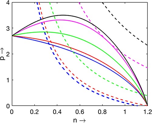
Based upon the nature of two nullclines $f_1(n,p)$ and $g_1(n,p)$, we find unique point of intersection between two non-trivial nullclines when $\frac{1}{1-h_1}<\kappa$. For $\frac{1}{1-h_1}>\kappa ,$ we find either two coexistence equilibrium or no feasible equilibrium. The situation changes from two coexistence equilibrium to no coexistence equilibrium through a saddle-node bifurcation (for details, see Section 2.2). The cases of 0, 1 and 2 coexistence equilibrium point are demonstrated in Figures 1 and 2. As is indicated in Figures 1 and 2 for two cases, one can observe the following two scenarios in terms of the changing patterns of the number of nontrivial equilibrium points by increasing magnitude of $h_1$:

Figure 1. Plots of two non-trivial nullclines $f_1(n,p)$ and $g_1(n,p)$ for $\sigma =0.5,\kappa =2,\alpha =1$ and $h_1$ varying from 0.1 to 0.6. As $h_1$ increases, the number of equilibrium point changes from 1 to 0.

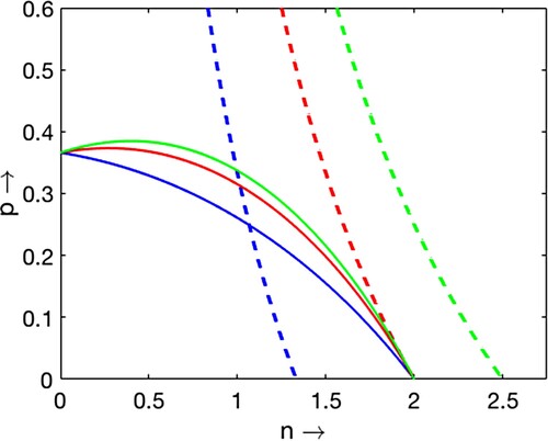
Figure 2. Plots of two non-trivial nullclines $f_1(n,p)$ and $g_1(n,p)$ for $\sigma =10,\kappa =1.2,\alpha =1$ and $h_1$ varying from 0.1 to 0.75. As $h_1$ increases, the number of equilibrium point changes from 1 to 0 ‘through 2’.

Scenario 1 ($\sigma =0.5$, Figure 1)

• When $h_1=0.25$ (Blue curves), there exists a unique coexistence equilibrium Theorem 2.1(i).

• When $h_1=0.5$ (Red curves), there exists a unique coexistence equilibrium at transcritical bifurcation threshold ($1-\frac{1}{\kappa (1-h_1)}=0$).

• When $h_1=0.6$ (Green curves), there are no coexistence equilibrium Theorem 2.1(ii) or (v).

Scenario 2 ($\sigma =10$, Figure 2)

• When $h_1=0.1$ (Blue curves), there exists a unique coexistence equilibrium Theorem 2.1(i).

• When $h_1=0.166666667$ (Red curves), there exists a unique coexistence equilibrium at transcritical bifurcation threshold ($1-\frac{1}{\kappa (1-h_1)}=0$).

• When $h_1=0.4$ (Green curves), there exist two coexistence equilibria Theorem 2.1(iii).

• When $h_1=0.66186$ (Magenta curves), there exists a unique instantaneous coexistence equilibrium at saddle-node bifurcation threshold Theorem 2.1(iv).

• When $h_1=0.75$ (Black curves), there are no coexistence equilibrium points Theorem 2.1(v).

For further increase in magnitude of $h_1$ leads to situation with no coexistence equilibrium. Now, for the positive equilibrium point $E_{+}(n_{\ast },p_{\ast })$, we can get the component $p_{\ast }$ by solving the second equation of (2) which is given as $p_{\ast }=\frac{h_1{n}_{\ast }-n_{\ast }+1}{\alpha n_{\ast }(1-h_1)}$ where $n_{\ast }$ is the positive root of the cubic equation given by $\mathrm{\alpha \sigma }(1-h_1)n^3-\mathrm{\alpha \kappa \sigma }(1-h_1)n^2-\kappa (1-h_1)n+\kappa =0.$In particular, for the existence of the coexistence equilibrium $E_{+}(n_{\ast },p_{\ast })$, the following theorem holds.

Theorem 2.1

The following statement holds true.

1. If $\kappa (1-h_1)>1$, the model (2) has a unique coexistence equilibrium.

2. If $\alpha \le \frac{1-h_1}{\sigma }$ and $\kappa (1-h_1)\le 1$, the model (2) has no coexistence equilibrium.

3. If $\alpha >\frac{1-h_1}{\sigma }$ and $\frac{1}{l\left(\frac{\mathrm{\alpha \sigma }}{1-h_1}\right)}<\kappa (1-h_1)\le 1$, the model (2) has two coexistence equilibria.

4. If $\alpha >\frac{1-h_1}{\sigma }$ and $\kappa (1-h_1)=\frac{1}{l\left(\frac{\mathrm{\alpha \sigma }}{1-h_1}\right)}\le 1$, the model (2) has a unique coexistence equilibrium.

5. If $\alpha >\frac{1-h_1}{\sigma }$ and $\kappa (1-h_1)<\frac{1}{l\left(\frac{\mathrm{\alpha \sigma }}{1-h_1}\right)}\le 1$, the model (2) has no coexistence equilibrium,

where the function l is positive and strictly monotone increasing on $[1,\mathrm{\infty }]$ defined as $l\left(u\right)=\frac{1}{3}+\frac{2}{3\sqrt{3}}\sqrt{u+\frac{1}{3}}+\frac{2}{27u}+\frac{2}{9\sqrt{3}u}\sqrt{u+\frac{1}{3}}\ge l\left(1\right)=1(u\ge 1).$

Proof.

When $h_1=0$, $n_{\ast }$ and $p_{\ast }$ satisfy the following equations: (4) $\sigma (1-\frac{n_{\ast }}{\kappa })-\frac{(1+\alpha p_{\ast })p_{\ast }}{1+h_1(1+\alpha p_{\ast })n_{\ast }}=0,\frac{(1+\alpha p_{\ast })n_{\ast }}{1+h_1(1+\alpha p_{\ast })n_{\ast }}-1=0.$(4) We note that (4(4) $\sigma (1-\frac{n_{\ast }}{\kappa })-\frac{(1+\alpha p_{\ast })p_{\ast }}{1+h_1(1+\alpha p_{\ast })n_{\ast }}=0,\frac{(1+\alpha p_{\ast })n_{\ast }}{1+h_1(1+\alpha p_{\ast })n_{\ast }}-1=0.$(4) ) yields $\sigma (1-\frac{1}{\kappa (1-h_1)(1+\alpha p_{\ast })})-(1-h_1)(1+\alpha p_{\ast })p_{\ast }=0$, that is, $\sigma (1-\frac{1}{\kappa (1-h_1)})+(\mathrm{\alpha \sigma }-(1-h_1\left)\right)p_{\ast }=2\alpha (1-h_1)(p_{\ast }{)}^2+{\alpha }^2(1-h_1\left)\right(p_{\ast }{)}^3$. Let us consider the case $\kappa (1-h_1)>1$. Since $1-\frac{1}{\kappa (1-h_1)}>0$, it is straightforward to prove that (i) holds true. Let us consider the case $\kappa (1-h_1)\le 1$, that is, $1-\frac{1}{\kappa (1-h_1)}\le 0$. If $\alpha \le \frac{1-h_1}{\sigma }$, then $\sigma (1-\frac{1}{\kappa (1-h_1)})+(\mathrm{\alpha \sigma }-(1-h_1\left)\right)p\le 0$ and $2\alpha (1-h_1)p^2+{\alpha }^2(1-h_1)p^3>0$ for all $p>0$. This implies that (ii) holds true. If $\alpha >\frac{1-h_1}{\sigma }$, let us define $w\left(p\right)=\sigma (1-\frac{1}{\kappa (1-h_1)})+(\mathrm{\alpha \sigma }-(1-h_1\left)\right)p-2\alpha (1-h_1)p^2-{\alpha }^2(1-h_1)p^3.$We note that $w\left(0\right)=\sigma (1-\frac{1}{\kappa (1-h_1)})\le 0$. By $w^{\mathrm{\prime }}\left(p\right)=(1-h_1)(\frac{\mathrm{\alpha \sigma }}{1-h_1}-1-4\mathrm{\alpha p}-3{\alpha }^2{p}^2)$, we have $\begin{array}{rl}w\left(p\right)& =\frac{1}{3}p{w}^{\mathrm{\prime }}\left(p\right)-\frac{2}{3}\alpha (1-h_1)p^2+\frac{2}{3}(\mathrm{\alpha \sigma }-(1-h_1\left)\right)p+\sigma (1-\frac{1}{\kappa (1-h_1)})\\ & =(\frac{1}{3}p+\frac{2}{9\alpha })w^{\mathrm{\prime }}\left(p\right)+(\frac{2}{3}\mathrm{\alpha \sigma }+\frac{2}{9}(1-h_1\left)\right)p\\ & -\frac{2}{9\alpha }(\mathrm{\alpha \sigma }-(1-h_1\left)\right)+\sigma (1-\frac{1}{\kappa (1-h_1)}).\end{array}$As $w^{\mathrm{\prime }}\left(p\right)=0$ if $p=-\frac{2}{3\alpha }+\sqrt{\frac{\frac{\mathrm{\alpha \sigma }}{1-h_1}+\frac{1}{3}}{3{\alpha }^2}}=:p^{+}>0$, the function w has a local maximum: $\begin{array}{rl}w\left(p^{+}\right)& =(\frac{2}{3}\mathrm{\alpha \sigma }+\frac{2}{9}(1-h_1\left)\right)(-\frac{2}{3\alpha }+\sqrt{\frac{\frac{\mathrm{\alpha \sigma }}{1-h_1}+\frac{1}{3}}{3{\alpha }^2}})\\ & -\frac{2}{9\alpha }(\mathrm{\alpha \sigma }-(1-h_1\left)\right)+\sigma (1-\frac{1}{\kappa (1-h_1)})\\ & =\sigma (\frac{1}{3}+\frac{2}{3\sqrt{3}}\sqrt{\frac{\mathrm{\alpha \sigma }}{1-h_1}+\frac{1}{3}}+\frac{2}{27\mathrm{\alpha \sigma }}(1-h_1)\\ & +\frac{2}{9\sqrt{3}\mathrm{\alpha \sigma }}(1-h_1)\sqrt{\frac{\mathrm{\alpha \sigma }}{1-h_1}+\frac{1}{3}}-\frac{1}{\kappa (1-h_1)})\\ & =\sigma (l\left(\frac{\mathrm{\alpha \sigma }}{1-h_1}\right)-\frac{1}{\kappa (1-h_1)})\end{array}$at $p=p^{+}$. Since the function $l\left(u\right)$ is positive and strictly monotone increasing in $u\ge 1$ (due to the fact that $(1+\frac{1}{3u})\sqrt{u+\frac{1}{3}}+\frac{1}{3\sqrt{3}u}=\frac{1}{u}\left(\right(u+\frac{1}{3}{)}^{\frac{3}{2}}+\frac{1}{3\sqrt{3}})$ is strictly monotone increasing in $u\ge 1$) with $l\left(u\right)>l\left(1\right)=1$ for all $u>1$, we obtain $l\left(\frac{\mathrm{\alpha \sigma }}{1-h_1}\right)>1$. This implies that $w\left(p^{+}\right)>0$ if $l\left(\frac{\mathrm{\alpha \sigma }}{1-h_1}\right)>\frac{1}{\kappa (1-h_1)}>1$ and $w\left(p^{+}\right)<0$ if $l\left(\frac{\mathrm{\alpha \sigma }}{1-h_1}\right)<\frac{1}{\kappa (1-h_1)}$. Therefore, $w\left(p\right)=0$ has two positive roots if $l\left(\frac{\mathrm{\alpha \sigma }}{1-h_1}\right)>\frac{1}{\kappa (1-h_1)}>1$ and no real roots if $l\left(\frac{\mathrm{\alpha \sigma }}{1-h_1}\right)<\frac{1}{\kappa (1-h_1)}$. In addition, $w\left(p\right)=0$ has a double real root if $l\left(\frac{\mathrm{\alpha \sigma }}{1-h_1}\right)=\frac{1}{\kappa (1-h_1)}$. Hence, the proof of (iii)–(v) is complete.

Remark 2.1

Theorem 2.1(ii) indicates that the predator cannot have a chance to coexist with the prey when the degree of cooperation among the predators is low.

Let us investigate the stability of equilibria. It is straightforward to prove that a trivial equilibrium $E_0$ is always unstable, because the Jacobian matrix for the model (2) evaluated at $E_0$ has at least one positive eigenvalue. The Jacobian matrix for the model (2) evaluated at $E_1$ is given by (5) $J_1=\left[\begin{array}{cc}-\sigma & {\displaystyle \frac{\kappa }{1+h_1\kappa }}\\ 0& {\displaystyle \frac{\kappa }{1+h_1\kappa }}-1\end{array}\right].$(5) $E_1$ is stable for $\frac{\kappa }{1+h_1\kappa }<1$ and is unstable otherwise. The predator-free equilibrium loses stability through a transcritical bifurcation at $h_{1_{\mathrm{TC}}}=1-\frac{1}{\kappa }$ (satisfying $\frac{\kappa }{1+h_{1_{\mathrm{TC}}}\kappa }-1=0$). In terms of $h_{1_{\mathrm{TC}}}$, $E_1$ is stable for $h_1>h_{1_{\mathrm{TC}}}$ and is unstable for $h_1<h_{1_{\mathrm{TC}}}$.

2.2. Saddle-node bifurcation

Now we prove that the system experiences a transition of having two coexistence equilibria from no coexistence equilibrium point or vice versa through saddle-node bifurcation by proving the required transversality conditions [40]. If $n_{\ast }$ denotes the first component of a feasible coexistence equilibrium point, then $n_{\ast }$ is a positive root of the cubic equation (6) $G\left(n\right)\equiv \mathrm{\sigma \alpha }(1-h_1)n^3-\mathrm{\sigma \alpha \kappa }(1-h_1)n^2-\kappa (1-h_1)n+\kappa =0.$(6) Let us assume that the equation $G\left(n\right)=0$ has a double root at the parametric threshold $h_{1_{\mathrm{SN}}}$ and the double root is denoted by $n_{02}$. Then the following conditions should be satisfied: (7) $G\left(n_{02}\right)=0,G^{\mathrm{\prime }}\left(n_{02}\right)=0,G^{\mathrm{\prime \prime }}\left(n_{02}\right)\ne 0.$(7) In terms of the non-trivial nullclines, we can say that the two curves $f_1(n,p)=0$ and $g_1(n,p)=0$ touch each other at $E_{\mathrm{SN}}(n_{02},p_{02})$ when $h_1=h_{1_{\mathrm{SN}}}$.

Evaluating the Jacobian matrix for the model (2) at $(n_{02},p_{02})$, we find (8) $J_{\mathrm{SN}}={\left[\begin{array}{cc}n{\displaystyle \frac{\mathrm{\partial }{f}_1}{\mathrm{\partial }n}}& n{\displaystyle \frac{\mathrm{\partial }{f}_1}{\mathrm{\partial }p}}\\ p{\displaystyle \frac{\mathrm{\partial }{g}_1}{\mathrm{\partial }n}}& p{\displaystyle \frac{\mathrm{\partial }{g}_1}{\mathrm{\partial }p}}\end{array}\right]}_{(n_{02},p_{02})}.$(8) Note that $f_1(n_{02},p_{02})=0$ and $g_1(n_{02},p_{02})=0$. Two curves $f_1(n,p)=0$ and $g_1(n,p)=0$ are tangential at $(n_{02},p_{02})$ implies (9) $-{\frac{\frac{\mathrm{\partial }{f}_1}{\mathrm{\partial }n}}{\frac{\mathrm{\partial }{f}_1}{\mathrm{\partial }p}}|}_{(n_{02},p_{02})}=-{\frac{\frac{\mathrm{\partial }{g}_1}{\mathrm{\partial }n}}{\frac{\mathrm{\partial }{g}_1}{\mathrm{\partial }p}}|}_{(n_{02},p_{02})}.$(9) Clearly, the Jacobian matrix $J_{\mathrm{SN}}$ has a zero eigenvalue. If V and W denote the eigenvectors of $J_{\mathrm{SN}}$ and $J_{\mathrm{SN}}^T$ respectively corresponding to zero eigenvalue then (10) $V=\left[\begin{array}{c}1\\ -{\displaystyle \frac{1+\alpha p_{02}}{\alpha n_{02}}}\end{array}\right],W=\left[\begin{array}{c}{\displaystyle \frac{\alpha p_{02}}{(1+\alpha p_{02}{)}^2{n}_{02}+\alpha p_{02}+1}}\\ 1\end{array}\right].$(10) Let $F=[f,g{]}^t$. Now we can calculate $\begin{array}{rl}& W^t{F}_{h_1}(E_{\mathrm{SN}};h_1=h_{1_{\mathrm{SN}}})\\ & =W^t{\left[\begin{array}{c}{\displaystyle \frac{\mathrm{\partial }f}{\mathrm{\partial }{h}_1}}\\ {\displaystyle \frac{\mathrm{\partial }g}{\mathrm{\partial }{h}_1}}\end{array}\right]}_{E_{\mathrm{SN}},h_{1_{\mathrm{SN}}}}\\ & =-\frac{(1+\alpha p_{02}{)}^3{n}_{02}^3{p}_{02}}{(1+h_{1_{\mathrm{SN}}}(1+\alpha p_{02}\left)n_{02}{)}^2\right((1+\alpha p_{02}{)}^2{n}_{02}+\alpha p_{02})}\ne 0,\end{array}$and $\begin{array}{rl}& W^t{D}^{2}F(E_{\mathrm{SN}};h_1=h_{1_{\mathrm{SN}}})(V,V)\\ & =W^t{\left[\begin{array}{c}{\displaystyle \frac{{\mathrm{\partial }}^{2}f}{\mathrm{\partial }{n}^2}}{v}_1^2+2{\displaystyle \frac{{\mathrm{\partial }}^{2}f}{\mathrm{\partial }n\mathrm{\partial p}}}{v}_1{v}_2+{\displaystyle \frac{{\mathrm{\partial }}^{2}f}{\mathrm{\partial }{p}^2}}{v}_2^2\\ {\displaystyle \frac{{\mathrm{\partial }}^{2}g}{\mathrm{\partial }{n}^2}}{v}_1^2+2{\displaystyle \frac{{\mathrm{\partial }}^{2}g}{\mathrm{\partial }n\mathrm{\partial p}}}{v}_1{v}_2+{\displaystyle \frac{{\mathrm{\partial }}^{2}g}{\mathrm{\partial }{p}^2}}{v}_2^2\end{array}\right]}_{E_{\mathrm{SN}},h_{1_{\mathrm{SN}}}}\\ & =\frac{\alpha p_{02}}{(1+\alpha p_{02}{)}^2{n}_{02}+\alpha p_{02}+1}(\frac{{\mathrm{\partial }}^{2}f}{\mathrm{\partial }{n}^2}{v}_1^2+2\frac{{\mathrm{\partial }}^{2}f}{\mathrm{\partial }n\mathrm{\partial p}}{v}_1{v}_2+\frac{{\mathrm{\partial }}^{2}f}{\mathrm{\partial }{p}^2}{v}_2^2)\\ & +(\frac{{\mathrm{\partial }}^{2}g}{\mathrm{\partial }{n}^2}{v}_1^2+2\frac{{\mathrm{\partial }}^{2}g}{\mathrm{\partial }n\mathrm{\partial p}}{v}_1{v}_2+\frac{{\mathrm{\partial }}^{2}g}{\mathrm{\partial }{p}^2}{v}_2^2)\\ & =\frac{2\kappa (1+\alpha p_{02})n_{02}+2\kappa (1-\alpha p_{02})(1-h_{1_{\mathrm{SN}}}{n}_{02})-2{\alpha }^2\sigma n_{02}^3{p}_{02}}{\mathrm{\alpha \kappa }{n}_{02}^3\left(\right(1+\alpha p_{02}{)}^2{n}_{02}+\alpha p_{02})}\ne 0.\end{array}$Hence all the transversality conditions for saddle-node bifurcation are satisfied. Figure 3 is the bifurcation diagram with respect to the parameter $h_1$ with $\sigma =10,\kappa =1.2,\alpha =1$.

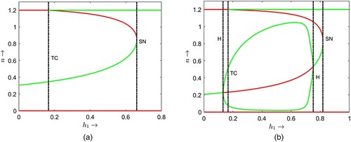
Figure 3. The bifurcation diagram with respect to the parameter $h_1$: (a) $\sigma =10,\kappa =1.2,\alpha =1$ and (b) $\sigma =10,\kappa =1.2,\alpha =2.217$.

2.3. Transcritical bifurcation

Proposition 2.2

A coexistence equilibrium point $E_{+}$ bifurcates from the prey only equilibrium point $E_1$ through transcritical bifurcation for the bifurcation parameter $h_1$ and at the bifurcation threshold $h_{1_{\mathrm{TC}}}=1-\frac{1}{\kappa }$, provided $\kappa >1$ holds.

Proof.

At $E_1$ and for $h_1=h_{1_{\mathrm{TC}}}$, Jacobian matrix of the model (2) is $J(E_1:h_1=h_{1_{\mathrm{TC}}})=\left[\begin{array}{cc}-\sigma & 1\\ 0& 0\end{array}\right].$It is evident that the Jacobian matrix has a simple zero eigenvalue. Now, corresponding to this zero eigenvalue, eigenvectors of the Jacobian matrix $J(E_1:h_{1_{\mathrm{TC}}}=1-\frac{1}{\kappa })$ and its transpose are evaluated as (11) $v=\left[\begin{array}{c}{\displaystyle \frac{1}{\sigma }}\\ 1\end{array}\right],w=\left[\begin{array}{c}0\\ 1\end{array}\right],$(11) respectively. Now, according to Sotomayor's conditions [40] the transversality conditions for transcritical bifurcation are $\begin{array}{rl}{w}^t{F}_{h_1}(E_1;h_1=h_{1_{\mathrm{TC}}})& =0,\\ w^{t}D{F}_{h_1}(E_1;h_1=h_{1_{\mathrm{TC}}})v& =-\frac{1}{(1+h_{1_{\mathrm{TC}}}{)}^2}\ne 0,\\ w^t{D}^{2}F(E_1;h_1=h_{1_{\mathrm{TC}}})(v,v)& ={(\frac{{\mathrm{\partial }}^{2}g}{\mathrm{\partial }{n}^2}\frac{1}{{\sigma }^2}+2\frac{{\mathrm{\partial }}^{2}g}{\mathrm{\partial }n\mathrm{\partial p}}\frac{1}{\sigma }+\frac{{\mathrm{\partial }}^{2}g}{\mathrm{\partial }{p}^2})|}_{E_1,h_{1_{\mathrm{TC}}}}\\ & =\frac{2}{(1+h_{1_{\mathrm{TC}}}{)}^2}(\frac{1}{\sigma }+\alpha )\ne 0.\end{array}$All of the transversality conditions hold here. As a result, we deduce from Sotomayor's theorem that a transcritical bifurcation occurs for the model (2) at $h_{1_{\mathrm{TC}}}=1-\frac{1}{\kappa }$.

2.4. Hopf bifurcation

The Jacobian matrix for the model (2) evaluated at $E_{+}$ is given by $\begin{array}{rl}{J}_{+}& =\left[\begin{array}{cl}\sigma (1-{\displaystyle \frac{2n_{\ast }}{\kappa }})-{\displaystyle \frac{1+\alpha p_{\ast }}{(1+h_1(1+\alpha p_{\ast })n_{\ast }{)}^2}}\cdot p_{\ast }& -{\displaystyle \frac{(1+\alpha p_{\ast })n_{\ast }}{1+h_1(1+\alpha p_{\ast })n_{\ast }}}\\ & -{\displaystyle \frac{\alpha n_{\ast }}{(1+h_1(1+\alpha p_{\ast })n_{\ast }{)}^2}}\cdot p_{\ast }\\ {\displaystyle \frac{1+\alpha p_{\ast }}{(1+h_1(1+\alpha p_{\ast })n_{\ast }{)}^2}}\cdot p_{\ast }& {\displaystyle \frac{(1+\alpha p_{\ast })n_{\ast }}{1+h_1(1+\alpha p_{\ast })n_{\ast }}}-1\\ & +{\displaystyle \frac{\alpha n_{\ast }}{(1+h_1(1+\alpha p_{\ast })n_{\ast }{)}^2}}\cdot p_{\ast }\end{array}\right]\\ & =\left[\begin{array}{cc}\sigma (1-{\displaystyle \frac{2n_{\ast }}{\kappa }})-p_{\ast }(1+\alpha p_{\ast })(1-h_1{)}^2& -1-\alpha n_{\ast }{p}_{\ast }(1-h_1{)}^2\\ p_{\ast }(1+\alpha p_{\ast })(1-h_1{)}^2& \alpha n_{\ast }{p}_{\ast }(1-h_1{)}^2\end{array}\right]\\ & =\left[\begin{array}{cc}\sigma (1-{\displaystyle \frac{2n_{\ast }}{\kappa }})-p_{\ast }(1+\alpha p_{\ast })(1-h_1{)}^2& -1-{\displaystyle \frac{\alpha p_{\ast }(1-h_1)}{1+\alpha p_{\ast }}}\\ p_{\ast }(1+\alpha p_{\ast })(1-h_1{)}^2& {\displaystyle \frac{\alpha p_{\ast }(1-h_1)}{1+\alpha p_{\ast }}}\end{array}\right].\end{array}$Moreover, $\begin{array}{rl}\sigma (1-\frac{2n_{\ast }}{\kappa })& =\frac{(1+\alpha p_{\ast })p_{\ast }}{1+h_1(1+\alpha p_{\ast })n_{\ast }}-\sigma \frac{n_{\ast }}{\kappa }\\ & =p_{\ast }(1-h_1)(1+\alpha p_{\ast })-\sigma \frac{1}{\kappa (1-h_1)(1+\alpha p_{\ast })}.\end{array}$This yields (12) $\begin{array}{rl}\mathrm{tr}{J}_{+}& =\sigma (1-\frac{2n_{\ast }}{\kappa })-(1+\alpha p_{\ast })p_{\ast }(1-h_1{)}^2+\frac{\alpha p_{\ast }(1-h_1)}{1+\alpha p_{\ast }}\\ & =(1+\alpha p_{\ast })p_{\ast }(1-h_1)h_1-\sigma \frac{1}{\kappa (1-h_1)(1+\alpha p_{\ast })}+\frac{\alpha p_{\ast }(1-h_1)}{1+\alpha p_{\ast }}\end{array}$(12) and (13) $\begin{array}{rl}det{J}_{+}& =\sigma (1-\frac{2n_{\ast }}{\kappa })\frac{\alpha p_{\ast }(1-h_1)}{1+\alpha p_{\ast }}+p_{\ast }(1+\alpha p_{\ast })(1-h_1{)}^2\\ & =\left(p_{\ast }\right(1-h_1\left)\right(1+\alpha p_{\ast })-\sigma \frac{1}{\kappa (1-h_1)(1+\alpha p_{\ast })})\frac{\alpha p_{\ast }(1-h_1)}{1+\alpha p_{\ast }}\\ & +p_{\ast }(1+\alpha p_{\ast })(1-h_1{)}^2.\end{array}$(13) The necessary conditions so that the model (2) undergoes a Hopf bifurcation at a positive equilibrium point $E_{+}$ is that $\mathrm{tr}{J}_{+}=0$ and $det{J}_{+}>0$, where $J_{+}$ is the Jacobian matrix evaluated at $E_{+}$. In fact, one can see that $det{J}_{+}>0$ is always valid when $h_1=0$ (see Appendix 2). Now from the condition $\mathrm{tr}{J}_{+}=0$, we have obtained the value of $h_1$ as $h_1^{\ast }=\frac{1}{2}\frac{\sqrt{\kappa }\sqrt{p_{\ast }}\sqrt{4{(\alpha p_{\ast }+1)}^3(\kappa -2n_{\ast })\sigma +{\alpha }^2\kappa p_{\ast }}+2p_{\ast }({\alpha }^2{p_{\ast }}^2+2\alpha p_{\ast }-\frac{\alpha }{2}+1)\kappa }{{(\alpha p_{\ast }+1)}^{2}k{p}_{\ast }}.$At $h_1=h_1^{\ast }$, the trace of the Jacobian matrix evaluated at $E_1$ is 0. Assume that the corresponding determinant of the Jacobian matrix evaluated at $E_1$ for the parametric value of $h_1=h_1^{\ast }$ is positive. Then the characteristic equation of the corresponding Jacobian matrix will have two purely imaginary eigenvalues $\pm i{h}_{1_0}$, where $h_{1_0}=\sqrt{det{J}_{+}{|}_{(E_{+},h_1=h_1^{\ast })}}.$The transversality condition for Hopf bifurcation at $E_{+}$ is given by ${\frac{\mathrm{d}\left(\mathrm{tr}{J}_{+}\right)}{\mathrm{d}{h}_1}|}_{h_1=h_1^{\ast }}=2(\alpha p_{\ast }+1)p_{\ast }(1-h_1^{\ast })-\frac{\alpha p_{\ast }}{\alpha p_{\ast }+1}\ne 0.$Therefore, the model (2) undergoes a Hopf bifurcation at the positive equilibrium point $E_{+}$ for the parametric value $h_1=h_1^{\ast }$.

2.4.1. Nature of Hopf bifurcating periodic solution

We need to derive the normal form of Hopf bifurcation to know about the direction and stability of the Hopf bifurcation. To derive the normal form, we first need to transform the positive equilibrium point to origin. Let us take the transformations $N=n-n_{\ast },P=p-p_{\ast }$. Using this transformations, the model (2) is transformed into $\begin{array}{rl}\frac{\mathrm{d}N}{\mathrm{d}t}& =(N+n_{\ast })(\sigma (1-\frac{N+n_{\ast }}{\kappa })-\frac{(1+\alpha (P+p_{\ast }))(P+p_{\ast })}{1+h(1+\alpha (P+p_{\ast }))(N+n_{\ast })})\equiv F(N,P),\\ \frac{\mathrm{d}P}{\mathrm{d}t}& =\frac{(N+n_{\ast })(1+\alpha (P+p_{\ast }))(P+p_{\ast })}{1+h(1+\alpha (P+p_{\ast }))(N+n_{\ast })}-P-p_{\ast }\equiv G(N,P).\end{array}$Taylor series expansion of $F(N,P)$ and $G(N,P)$ at $(N,P)=(0,0)$ up to order 3 gives $\begin{array}{rl}\frac{\mathrm{d}N}{\mathrm{d}t}& =a_{10}N+a_{01}P+a_{11}\mathrm{NP}+a_{20}{N}^2+a_{02}{P}^2\\ & +a_{30}{N}^3+a_{21}{N}^{2}P+a_{12}N{P}^2+a_{03}{P}^3+O\left(|N{|}^4\right),\\ \frac{\mathrm{d}P}{\mathrm{d}t}& =b_{10}N+b_{01}P+b_{11}\mathrm{NP}+b_{20}{N}^2+b_{02}{P}^2\\ & +b_{30}{N}^3+b_{21}{N}^{2}P+b_{12}N{P}^2+b_{03}{P}^3+O\left(|P{|}^4\right).\end{array}$The expressions of $a_{\mathrm{ij}}$ and $b_{\mathrm{ij}}$ are given in Appendix 3. Neglecting the higher order terms of degree 4 and above, the system of equations transform into (14) $\dot{Z}=J_{E_{\ast }}Z+A\left(Z\right),$(14) where $Z=\left[\begin{array}{c}N\\ P\end{array}\right]$ and $\left[\begin{array}{c}{A}_1\\ A_2\end{array}\right]=\left[\begin{array}{c}{a}_{11}\mathrm{NP}+a_{20}{N}^2+a_{02}{P}^2+a_{30}{N}^3+a_{21}{N}^{2}P+a_{12}N{P}^2+a_{03}{P}^3\\ b_{11}\mathrm{NP}+b_{20}{N}^2+b_{02}{P}^2+b_{30}{N}^3+b_{21}{N}^{2}P+b_{12}N{P}^2+b_{03}{P}^3\end{array}\right].$The eigenvector w of the Jacobian matrix $J_{E_{+}}$ with respect to the eigenvalue $i{h}_{1_0}$ when $h_1=h_1^{\ast }$ is $w=\left[\begin{array}{c}{a}_{01}\\ i{h}_{1_0}-a_{10}\end{array}\right].$Define $Q=\left[\mathrm{\Re }\right(w),\mathrm{\Im }(w\left)\right]=\left[\begin{array}{cc}{a}_{01}& 0\\ -a_{10}& h_{1_0}\end{array}\right].$Take Z = QX or $X=Q^{-1}Z$, where $X=\left[\begin{array}{c}{X}_1\\ X_2\end{array}\right]$. These transformations transform the system into the following equation: $\dot{X}=\left(Q^{-1}{J}_{E_{\ast }}Q\right)X+Q^{-1}A\left(\mathrm{QX}\right),$that is, $\left[\begin{array}{c}\dot{X_1}\\ \dot{X_2}\end{array}\right]=\left[\begin{array}{cc}0& -h_{1_0}\\ h_{1_0}& 0\end{array}\right]\left[\begin{array}{c}{X}_1\\ X_2\end{array}\right]+\left[\begin{array}{c}{N}^1(X_1,X_2;h_1=h_1^{\ast })\\ N^2(X_1,X_2;h_1=h_1^{\ast })\end{array}\right].$$N^1$ and $N^2$ are non-linear functions in the variable $X_1$ and $X_2$ and the corresponding forms are $\begin{array}{rl}{N}^1(X_1,X_2;h_1=h_1^{\ast })& =\frac{A_1}{a_{01}},\\ N^2(X_1,X_2;h_1=h_1^{\ast })& =-\frac{a_{10}{A}_1+a_{01}{A}_2}{h_{1_0}{a}_{01}}.\end{array}$The expression of $A_1$ and $A_2$ are given in Appendix 3.

To confer about the direction and stability of the bifurcated periodic solution, it is necessary to compute the first Lyapunov coefficient ($l_1$) which is computed as below $\begin{array}{rl}{l}_1& =\frac{1}{16}{[N_{X_1{X}_1{X}_1}^1+N_{X_1{X}_2{X}_2}^1+N_{X_1{X}_1{X}_2}^1+N_{X_2{X}_2{X}_2}^1]}_{(0,0;h_{1_0})}\\ & +\frac{1}{16h_{1_0}}[N_{X_1{X}_2}^1(N_{X_1{X}_1}^1+N_{X_2{X}_2}^1)-N_{X_1{X}_2}^2(N_{X_1{X}_2}^2+N_{X_2{X}_2}^2)\\ & -N_{X_1{X}_1}^1{N}_{X_1{X}_1}^2+N_{X_2{X}_2}^1{N}_{X_2{X}_2}^2{]}_{(0,0;h_{1_0})}.\end{array}$The Hopf bifurcation is supercritical if $l_1<0$ and subcritical if $l_1>0$. For $l_1=0$, the system experiences a generalized Hopf bifurcation.

3. Delayed model

In this section, we consider the delayed model corresponding to the model (2) by introducing maturation time delay in predator growth. The maturation time delay is the time required for the juvenile predator individuals to become adult and capable to contribute to the growth of their own population [16,41–44]. With the maturation delay parameter τ, we can define the delayed model (15a) $\begin{array}{rl}\frac{\mathrm{d}n\left(t\right)}{\mathrm{d}t}& =n\left(t\right)(\sigma (1-\frac{n\left(t\right)}{\kappa })-\frac{(1+\mathrm{\alpha p}(t\left)\right)p\left(t\right)}{1+h_1(1+\mathrm{\alpha p}(t\left)\right)n\left(t\right)}),\end{array}$(15a) (15b) $\begin{array}{rl}\frac{\mathrm{d}p\left(t\right)}{\mathrm{d}t}& =\exp (-\text{β}\tau )\frac{(1+\mathrm{\alpha p}(t-\tau \left)\right)n(t-\tau )}{1+h_1(1+\mathrm{\alpha p}(t-\tau \left)\right)n(t-\tau )}p(t-\tau )-p\left(t\right),\end{array}$(15b) where β is the dimensionless mortality rate of the juvenile predators (see [16,45,46] for derivation of the delayed model). Both the parameters τ and β are positive and dimensionless. Juvenile predators survive at a rate $\exp (-\text{β}\tau )$ and the proportion of juvenile predators that were able to survive over the time period $[t-\tau ,t]$ is added to the adult predator class at time t. It should be observed that juvenile predator density $p_j$ is not appearing in the growth equation for prey and growth equation for adult predator. Therefore, growth equation for juvenile predator can be decoupled. The growth equation for juvenile predators can be rewritten (for detail see [46,47]) as follows: $p_j\left(t\right)={\int }_{-\tau }^0\frac{(1+\mathrm{\alpha p}(t+u\left)\right)n(t+u)p(t+u)}{1+h_1(1+\mathrm{\alpha p}(t+u\left)\right)n(t+u)}\mathrm{d}u,$and $p_j\left(0\right)$ is given by $p_j\left(0\right)={\int }_{-\tau }^0\frac{(1+\mathrm{\alpha p}(u\left)\right)n\left(u\right)p\left(u\right)}{1+h_1(1+\mathrm{\alpha p}(u\left)\right)n\left(u\right)}\mathrm{d}u.$As $n\left(t\right)$, $p\left(t\right)$ completely determines the juvenile class $p_j\left(t\right)$; therefore, we only consider the model (15) for our further study (for detail derivation, see [16,45]). The delayed model is subjected to the non-negative continuous history functions $n\left(s\right),p\left(s\right)\ge 0$ for $-\tau \le s\le 0$. Here $n\left(s\right)$ and $p\left(s\right)$ are two continuous non-negative functions of s for $s\in [-\tau ,0]$. Along with the similar discussion in Proposition A.1 in Appendix 1, one can obtain the well-posedness of the model (15).

3.1. Equilibria and stability

Similar to Theorem 2.1, for the existence of the coexistence equilibrium point $E_{+}(n_{\ast },p_{\ast })$ of the model (15), the following theorem holds.

Theorem 3.1

The following statement holds true.

1. If $\kappa (\exp (-\text{β}\tau )-h_1)>1$, the model (15) has a unique coexistence equilibrium.

2. If $\alpha \le \frac{1-h_1\exp \left(\text{β}\tau \right)}{\sigma }$ and $\kappa (\exp (-\text{β}\tau )-h_1)\le 1$, the model (15) has no coexistence equilibrium.

3. If $\alpha >\frac{1-h_1\exp \left(\text{β}\tau \right)}{\sigma }$ and $\frac{1}{l\left(\frac{\mathrm{\alpha \sigma }}{1-h_1\exp \left(\text{β}\tau \right)}\right)}<\kappa (\exp (-\text{β}\tau )-h_1)\le 1$, the model (15) has two coexistence equilibria.

4. If $\alpha >\frac{1-h_1\exp \left(\text{β}\tau \right)}{\sigma }$ and $\kappa (\exp (-\text{β}\tau )-h_1)=\frac{1}{l\left(\frac{\mathrm{\alpha \sigma }}{1-h_1\exp \left(\text{β}\tau \right)}\right)}\le 1$, the model (15) has a unique coexistence equilibrium.

5. If $\alpha >\frac{1-h_1\exp \left(\text{β}\tau \right)}{\sigma }$ and $\kappa (\exp (-\text{β}\tau )-h_1)<\frac{1}{l\left(\frac{\mathrm{\alpha \sigma }}{1-h_1\exp \left(\text{β}\tau \right)}\right)}\le 1$, the model (15) has no coexistence equilibrium,

where $l\left(u\right)$ is defined in Theorem 2.1.

Proof.

One can see that $n_{\ast }$ and $p_{\ast }$ satisfy the following equations: (16) $\sigma (1-\frac{n_{\ast }}{\kappa })-\frac{(1+\alpha p_{\ast })p_{\ast }}{1+h_1(1+\alpha p_{\ast })n_{\ast }}=0,\exp (-\text{β}\tau )\frac{(1+\alpha p_{\ast })n_{\ast }}{1+h_1(1+\alpha p_{\ast })n_{\ast }}-1=0.$(16) We note that (16(16) $\sigma (1-\frac{n_{\ast }}{\kappa })-\frac{(1+\alpha p_{\ast })p_{\ast }}{1+h_1(1+\alpha p_{\ast })n_{\ast }}=0,\exp (-\text{β}\tau )\frac{(1+\alpha p_{\ast })n_{\ast }}{1+h_1(1+\alpha p_{\ast })n_{\ast }}-1=0.$(16) ) yields $\sigma (1-\frac{1}{\kappa (\exp (-\text{β}\tau )-h_1)(1+\alpha p_{\ast })})-(1-h_1\exp (\text{β}\tau \left)\right)(1+\alpha p_{\ast })p_{\ast }=0$, that is, $\begin{array}{rl}& \sigma (1-\frac{1}{\kappa (\exp (-\text{β}\tau )-h_1)})+(\mathrm{\alpha \sigma }-(1-h_1\exp \left(\text{β}\tau \right)\left)\right)p_{\ast }\\ & =2\alpha (1-h_1\exp (\text{β}\tau \left)\right)(p_{\ast }{)}^2+{\alpha }^2(1-h_1\exp \left(\text{β}\tau \right)\left)\right(p_{\ast }{)}^3.\end{array}$Let us consider the case $\kappa (\exp (-\text{β}\tau )-h_1)>1$. Since $1-\frac{1}{\kappa (\exp (-\text{β}\tau )-h_1)}>0$, it is straightforward to prove that (i) holds true. Let us consider the case $\kappa (\exp (-\text{β}\tau )-h_1)\le 1$, that is, $1-\frac{1}{\kappa (\exp (-\text{β}\tau )-h_1)}\le 0$. If $\alpha \le \frac{1-h_1\exp \left(\text{β}\tau \right)}{\sigma }$, then $\sigma (1-\frac{1}{\kappa (\exp (-\text{β}\tau )-h_1)})+(\mathrm{\alpha \sigma }-(1-h_1\exp \left(\text{β}\tau \right)\left)\right)p_{\ast }\le 0$ and $2\alpha p^2+{\alpha }^2{p}^3>0$ for all $p>0$. This implies that (ii) holds true. If $\alpha >\frac{1-h_1\exp \left(\text{β}\tau \right)}{\sigma }$, let us define $\begin{array}{rl}{w}_{\tau }\left(p\right)& =\sigma (1-\frac{1}{\kappa (\exp (-\text{β}\tau )-h_1)})+(\mathrm{\alpha \sigma }-(1-h_1\exp \left(\text{β}\tau \right)\left)\right)p_{\ast }\\ & -2\alpha (1-h_1\exp (\text{β}\tau \left)\right)p^2-{\alpha }^2(1-h_1\exp (\text{β}\tau \left)\right)p^3.\end{array}$We note that $w_{\tau }\left(0\right)=\sigma (1-\frac{1}{\kappa (\exp (-\text{β}\tau )-h_1)})\le 0$. By $w_{\tau }^{\mathrm{\prime }}\left(p\right)=\mathrm{\alpha \sigma }-(1-h_1\exp (\text{β}\tau \left)\right)-4\alpha (1-h_1\exp (\text{β}\tau \left)\right)p-3{\alpha }^2(1-h_1\exp (\text{β}\tau \left)\right)p^2$ and the similar discussion in the proof of Theorem 2.1, one can see that $w_{\tau }\left(p\right)=0$ has two positive roots if $\frac{1}{l\left(\frac{\mathrm{\alpha \sigma }}{1-h_1\exp \left(\text{β}\tau \right)}\right)}<\kappa (\exp (-\text{β}\tau )-h_1)$ and no real roots if $\frac{1}{l\left(\frac{\mathrm{\alpha \sigma }}{1-h_1\exp \left(\text{β}\tau \right)}\right)}>\kappa (\exp (-\text{β}\tau )-h_1)$. In addition, $w_{\tau }\left(p\right)=0$ has a double real root if $\kappa (\exp (-\text{β}\tau )-h_1)=\frac{1}{l\left(\frac{\mathrm{\alpha \sigma }}{1-h_1\exp \left(\text{β}\tau \right)}\right)}$. Hence, the proof of (iii)–(v) is complete.

Let us investigate the stability of equilibria. It is straightforward to prove that a trivial equilibrium $E_0$ is always unstable, because the Jacobian matrix for the model (15) evaluated at $E_0$ has at least one positive eigenvalue. The Jacobian matrix for the model (15) evaluated at $E_1$ is given by $det(J_{1\tau }-\mathrm{\lambda I})=0,$where $J_{1\tau }=\left[\begin{array}{cc}-\sigma & {\displaystyle \frac{\kappa }{1+h_1\kappa }}\\ 0& \exp (-(\text{β}+\lambda \left)\tau \right){\displaystyle \frac{\kappa }{1+h_1\kappa }}-1\end{array}\right].$Therefore $E_1$ is stable for $\exp (-\text{β}\tau )\frac{\kappa }{1+h_1\kappa }<1$ and is unstable otherwise.

3.2. Delay-induced Hopf bifurcation

The linearization of the model (15) around $E_{+}$ gives us the following equivalent system in the vicinity of the positive equilibrium point: $\begin{array}{rl}\frac{\mathrm{d}u}{\mathrm{d}t}& ={\varphi }_{1}u\left(t\right)+{\varphi }_{2}v\left(t\right),\\ \frac{\mathrm{d}v}{\mathrm{d}t}& ={\psi }_{1}u(t-\tau )+{\psi }_{2}v(t-\tau )+{\psi }_{3}v\left(t\right),\end{array}$where $\begin{array}{rl}{\varphi }_1& =\frac{n_{\ast }(1+\alpha p_{\ast })(-\sigma n_{\ast }^2+\kappa p_{\ast })-\kappa p_{\ast }}{\kappa n_{\ast }^2(1+\alpha p_{\ast })},{\varphi }_2=\frac{-n_{\ast }(1+\alpha p_{\ast }{)}^2-\alpha p_{\ast }}{n_{\ast }(1+\alpha p_{\ast }{)}^2},\\ {\psi }_1& =\frac{p_{\ast }}{n_{\ast }^2(1+\alpha p_{\ast })},{\psi }_2=\frac{n_{\ast }+(2n_{\ast }+1)\alpha p_{\ast }+{\alpha }^2{n}_{\ast }{p}_{\ast }^2}{n_{\ast }(1+\alpha p_{\ast }{)}^2},{\psi }_3=-1.\end{array}$The associated characteristic equation is (17) $\mathrm{{\rm Y}}(\lambda ,\tau )={\lambda }^2-({\varphi }_1+{\psi }_3)\lambda +{\varphi }_1{\psi }_3+{\mathrm{e}}^{-\mathrm{\lambda \tau }}({\varphi }_1{\psi }_2-{\varphi }_2{\psi }_1-{\psi }_2\lambda )=0.$(17) For simplicity, let $\mathrm{{\rm Y}}(\lambda ,\tau )={\mathrm{{\rm Y}}}_1(\lambda ,\tau )+{\mathrm{e}}^{-\mathrm{\lambda \tau }}{\mathrm{{\rm Y}}}_2(\lambda ,\tau )$, where ${\mathrm{{\rm Y}}}_1(\lambda ,\tau )={\lambda }^2-({\varphi }_1+{\psi }_3)\lambda +{\varphi }_1{\psi }_3$ and ${\mathrm{{\rm Y}}}_2(\lambda ,\tau )=({\varphi }_1{\psi }_2-{\varphi }_2{\psi }_1-{\psi }_2\lambda )$.

To examine the occurrence of delay-induced Hopf bifurcation, specifically to determine the conditions under which a pair of purely imaginary eigenvalues of the characteristic equation (17(17) $\mathrm{{\rm Y}}(\lambda ,\tau )={\lambda }^2-({\varphi }_1+{\psi }_3)\lambda +{\varphi }_1{\psi }_3+{\mathrm{e}}^{-\mathrm{\lambda \tau }}({\varphi }_1{\psi }_2-{\varphi }_2{\psi }_1-{\psi }_2\lambda )=0.$(17) ) exist, we can substitute $\lambda =\mathrm{i\omega }$ in (17(17) $\mathrm{{\rm Y}}(\lambda ,\tau )={\lambda }^2-({\varphi }_1+{\psi }_3)\lambda +{\varphi }_1{\psi }_3+{\mathrm{e}}^{-\mathrm{\lambda \tau }}({\varphi }_1{\psi }_2-{\varphi }_2{\psi }_1-{\psi }_2\lambda )=0.$(17) ) which gives ${\mathrm{{\rm Y}}}_1(\mathrm{i\omega },\tau )+{\mathrm{e}}^{-\mathrm{i\omega \tau }}{\mathrm{{\rm Y}}}_2(\mathrm{i\omega },\tau )=0,$where $\omega \in {\mathbb{R}}_{+}$ and $\mathrm{{\rm Y}}(\mathrm{i\omega },\tau )=0$. Sorting out the real and imaginary portions, we have $\begin{array}{rl}& {\mathrm{{\rm Y}}}_{1R}(\mathrm{i\omega },\tau )+{\mathrm{{\rm Y}}}_{2R}(\mathrm{i\omega },\tau )\cos \mathrm{\omega \tau }+{\mathrm{{\rm Y}}}_{2I}(\mathrm{i\omega },\tau )\sin \mathrm{\omega \tau }=0,\\ & {\mathrm{{\rm Y}}}_{1I}(\mathrm{i\omega },\tau )+{\mathrm{{\rm Y}}}_{2I}(\mathrm{i\omega },\tau )\cos \mathrm{\omega \tau }-{\mathrm{{\rm Y}}}_{2R}(\mathrm{i\omega },\tau )\sin \mathrm{\omega \tau }=0,\end{array}$where R and I indicate the real and imaginary parts of the corresponding components, respectively. As a result, we get (18) $\begin{array}{rl}\sin \left(\mathrm{\omega \tau }\right)& =\frac{{\mathrm{{\rm Y}}}_{1I}(\mathrm{i\omega },\tau ){\mathrm{{\rm Y}}}_{2R}(\mathrm{i\omega },\tau )-{\mathrm{{\rm Y}}}_{1R}(\mathrm{i\omega },\tau ){\mathrm{{\rm Y}}}_{2I}(\mathrm{i\omega },\tau )}{{\mathrm{{\rm Y}}}_{2R}^2(\mathrm{i\omega },\tau )+{\mathrm{{\rm Y}}}_{2I}^2(\mathrm{i\omega },\tau )},\end{array}$(18) (19) $\begin{array}{rl}\cos \left(\mathrm{\omega \tau }\right)& =-\frac{{\mathrm{{\rm Y}}}_{1R}(\mathrm{i\omega },\tau ){\mathrm{{\rm Y}}}_{2R}(\mathrm{i\omega },\tau )+{\mathrm{{\rm Y}}}_{1I}(\mathrm{i\omega },\tau ){\mathrm{{\rm Y}}}_{2I}(\mathrm{i\omega },\tau )}{{\mathrm{{\rm Y}}}_{2R}^2(\mathrm{i\omega },\tau )+{\mathrm{{\rm Y}}}_{2I}^2(\mathrm{i\omega },\tau )}.\end{array}$(19) Assume that there is a common solution $\theta \left(\tau \right)$ for both Equations (18(18) $\begin{array}{rl}\sin \left(\mathrm{\omega \tau }\right)& =\frac{{\mathrm{{\rm Y}}}_{1I}(\mathrm{i\omega },\tau ){\mathrm{{\rm Y}}}_{2R}(\mathrm{i\omega },\tau )-{\mathrm{{\rm Y}}}_{1R}(\mathrm{i\omega },\tau ){\mathrm{{\rm Y}}}_{2I}(\mathrm{i\omega },\tau )}{{\mathrm{{\rm Y}}}_{2R}^2(\mathrm{i\omega },\tau )+{\mathrm{{\rm Y}}}_{2I}^2(\mathrm{i\omega },\tau )},\end{array}$(18) ) and (19(19) $\begin{array}{rl}\cos \left(\mathrm{\omega \tau }\right)& =-\frac{{\mathrm{{\rm Y}}}_{1R}(\mathrm{i\omega },\tau ){\mathrm{{\rm Y}}}_{2R}(\mathrm{i\omega },\tau )+{\mathrm{{\rm Y}}}_{1I}(\mathrm{i\omega },\tau ){\mathrm{{\rm Y}}}_{2I}(\mathrm{i\omega },\tau )}{{\mathrm{{\rm Y}}}_{2R}^2(\mathrm{i\omega },\tau )+{\mathrm{{\rm Y}}}_{2I}^2(\mathrm{i\omega },\tau )}.\end{array}$(19) ), and that $0\le \theta \left(\tau \right)<2\pi$. With this, we may deduce that ${\tau }_0=\frac{\theta \left(\tau \right)}{\omega }$ is the smallest Hopf bifurcation threshold. Solving the equation ${\displaystyle \tau ={\tau }_n\left(\tau \right)}$ yields the consecutive Hopf bifurcation thresholds ${\tau }_c$ when switching of stability occurs where ${\tau }_n\left(\tau \right)$ is the general solution of Equations (18(18) $\begin{array}{rl}\sin \left(\mathrm{\omega \tau }\right)& =\frac{{\mathrm{{\rm Y}}}_{1I}(\mathrm{i\omega },\tau ){\mathrm{{\rm Y}}}_{2R}(\mathrm{i\omega },\tau )-{\mathrm{{\rm Y}}}_{1R}(\mathrm{i\omega },\tau ){\mathrm{{\rm Y}}}_{2I}(\mathrm{i\omega },\tau )}{{\mathrm{{\rm Y}}}_{2R}^2(\mathrm{i\omega },\tau )+{\mathrm{{\rm Y}}}_{2I}^2(\mathrm{i\omega },\tau )},\end{array}$(18) ) and (19(19) $\begin{array}{rl}\cos \left(\mathrm{\omega \tau }\right)& =-\frac{{\mathrm{{\rm Y}}}_{1R}(\mathrm{i\omega },\tau ){\mathrm{{\rm Y}}}_{2R}(\mathrm{i\omega },\tau )+{\mathrm{{\rm Y}}}_{1I}(\mathrm{i\omega },\tau ){\mathrm{{\rm Y}}}_{2I}(\mathrm{i\omega },\tau )}{{\mathrm{{\rm Y}}}_{2R}^2(\mathrm{i\omega },\tau )+{\mathrm{{\rm Y}}}_{2I}^2(\mathrm{i\omega },\tau )}.\end{array}$(19) ) given by ${\tau }_n\left(\tau \right)=\frac{\theta \left(\tau \right)+2\mathrm{n\pi }}{\omega },n=0,1,2,\dots .$The least value of ${\tau }_n\left(\tau \right)$ gives us the desired Hopf bifurcation threshold.

3.3. Numerical saddle-node bifurcation results

We need to check the change in shape and position of the non-trivial predator nullcline with the variation of τ. The non-trivial predator nullcline is (20) $g_1(n,p,\tau ):=\exp (-\text{β}\tau )\frac{(1+\mathrm{\alpha p})n}{1+h_1(1+\mathrm{\alpha p})n}-1=0.$(20) This curve intersects n-axis at $(\frac{1}{\exp (-\text{β}\tau )-h_1},0)$ and to be relevant in the context of ecology, we should have $h_1<\exp (-\text{β}\tau )$. Solving above equation for p, we can write $p=\frac{1-\exp (-\text{β}\tau )n+h_{1}n}{\alpha (\exp (-\text{β}\tau )-h_1)n}$since it follows from (20(20) $g_1(n,p,\tau ):=\exp (-\text{β}\tau )\frac{(1+\mathrm{\alpha p})n}{1+h_1(1+\mathrm{\alpha p})n}-1=0.$(20) ) that $1+\mathrm{\alpha p}=\frac{1}{(\exp (-\text{β}\tau )-h_1)n}$. If we differentiate this equation with respect to n, we find $\frac{\mathrm{d}p}{\mathrm{d}n}=-\frac{1}{\alpha (\exp (-\text{β}\tau )-h_1)n^2}<0,$for $n>0$ and $0<h_1<\exp (-\text{β}\tau )$. Clearly the non-trivial predator nullcline passes through $(\frac{1}{\exp (-\text{β}\tau )-h_1},0)$, has vertical asymptote n = 0 and is monotone decreasing in the first quadrant.

Based upon the nature of two nullclines, we find unique point of intersection between two non-trivial nullclines when $\frac{1}{\exp (-\text{β}\tau )-h_1}<\kappa$. For $\frac{1}{\exp (-\text{β}\tau )-h_1}>\kappa$ we find either two coexistence equilibria or no feasible equilibrium. The situation changes from two coexistence equilibria to no feasible equilibrium through a saddle-node bifurcation.

4. Numerical results

Here, using numerical examples, we numerically illustrate the bifurcation results associated with the considered model dynamics. The positions of nullclines are significantly affected by the parameters $h_1$ and α, which also have an impact on the stability of the equilibrium point. As a result, the parameters $h_1$ and α are an obvious choice for bifurcation parameters. It should be noted that the inclusion of the delay parameter in the expression of the non-trivial predator nullcline results in a new dependence between the parameter τ and the number and location of interior equilibrium points.

Figure 3 is a one parameter bifurcation diagram where we choose $h_1$ as the bifurcation parameter and for two fixed but different values of parameter α. In both cases, the non-delayed system (2) has exactly one positive equilibrium point before the transcritical threshold value $h_1=0.1667$. The extinction state $E_0$ is always unstable for any permissible value of $h_1$, implying that the system can never settle down in the extinction state. The prey only equilibrium point $E_1$ remains unstable before the transcritical bifurcation threshold value $h_1=0.1667$. These results show that the coexistence equilibrium point becomes the only attractor, implying that the system is globally stable at the positive equilibrium point up to the transcritical threshold value $h_1=0.1667$. The system experiences coexistence in two positive equilibrium points for $0.1667<h_1<0.661$ when $\alpha =1$ and $0.1667<h_1<0.818$ when $\alpha =2.217$ after which the coexistence lost through saddle-node bifurcation. For $\alpha =1$, $h_1$ induces a bi-stability situation between one coexistence equilibrium point and the prey only equilibrium point. The basin of attractions of these two attractors is separated by the stable manifold of a coexistence equilibrium which is a saddle point.

For $\alpha =2.217$, we observe two types of bi-stability. The first type is node-cycle bi-stability which occurs between a locally stable positive equilibrium point and a locally stable limit cycle when $h_1$ crosses the transcritical bifurcation threshold 0.1667. The second type is node–node bi-stability which occurs between the prey only equilibrium point and a coexistence equilibrium point when $h_1$ crosses the Hopf bifurcation threshold 0.752 and continues up to saddle node bifurcation threshold 0.818. After the saddle-node bifurcation, the prey only equilibrium point $E_1$ becomes the only stable attractor of the system implying $E_0$ becomes globally stable. These imply that, in the case of cooperative hunting among predators, less hunting time is advantageous for the coexistence of prey and their predators. On the other hand, the system will eventually enter a predator extinction state if the predators require more time to hunt their prey. Note that increasing the value of α induces Hopf bifurcations in the model dynamics through which the prey and their predators start to coexist in oscillatory mode for some intermediate value of hunting cooperation parameter $h_1$.

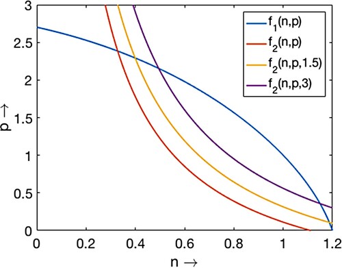
The model analysis for the delayed system (15) reveals that the number of positive equilibrium points has a dependence on the magnitude of the delay parameter τ. We can check the plots of the non-trivial nullcline for a representative set of parameter values $\sigma =10$, $\kappa =1.2$, $\alpha =1$, $h_1=0.1$, $\text{β}=0.1$ and different values of τ. Plots of the non-trivial predator nullcline $g_1(n,p,\tau )$ for three different values of τ are in Figure 4. Now we are interested to understand the shifting of bifurcation thresholds with the variation of the delay parameter τ.

Figure 4. Plots of non-trivial prey nullcline $f_1(n,p)$ and predator nullcline $g_1(n,p,\tau )$ for $\sigma =10$, $\kappa =1.2$, $\alpha =1$, $h_1=0.1$, $\text{β}=0.1$ and three different values of τ: $\tau =0$, $\tau =1.5$, $\tau =3$.

Two bifurcation diagrams are presented in Figure 5 with respect to the parameter $h_1$ and some different but fixed values of the delay parameter τ as mentioned at the caption of the figure. If we compare the bifurcation thresholds between the Figures 3(a) and 5, we find that the transcritical bifurcation threshold shifts from $0.1667(\tau =0)$ to $0.02737(\tau =0.3,\text{β}=0.5)$ and the saddle-node bifurcation threshold shifts from $0.661(\tau =0)$ to $0.485(\tau =0.3,\text{β}=0.5)$ to $0.326(\tau =0.6,\text{β}=0.5)$. Note that less hunting time is required to induce the dynamical shift from single coexistence to double coexistence and from double coexistence to no coexistence if juvenile predators require longer maturation times. Similar comparisons can be made between the thresholds in Figures 3(b) and 6(a) for transcritical, saddle-node and Hopf bifurcations. For $\alpha =2.217$, we find that the first Hopf bifurcation threshold shifts from $0.132(\tau =0)$ to $0.044(\tau =0.05,\text{β}=0.1)$. The transcritical bifurcation threshold shifts from $0.1667(\tau =0)$ to $0.1617(\tau =0.05,\text{β}=0.1)$. Second Hopf bifurcation threshold shifts from $0.752(\tau =0)$ to $0.748(\tau =0.05,\text{β}=0.1)$. The saddle node bifurcation threshold shifts from $0.818(\tau =0)$ to $0.812(\tau =0.05,\text{β}=0.1)$. It is worth noting that increasing the magnitude of the delay causes all of the above bifurcations to occur for a lower value of the parameter $h_1$ (see Figures 6b, 7 and 8). It is noted that for an increased maturation time of juvenile predators, reduced hunting time induces the system to exhibit oscillatory coexistence and further ruling out the oscillations to have steady-state coexistence of prey and their predators.

Figure 5. The bifurcation diagram with respect to the parameter $h_1$ with $\sigma =10$, $\kappa =1.2$, $\alpha =1$, $\text{β}=0.5$: (a) $\tau =0.3$ and (b) $\tau =0.6$.

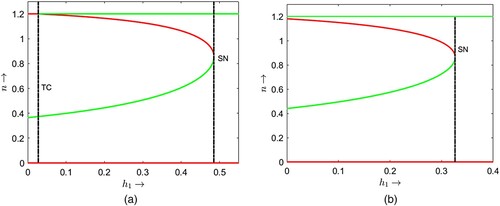
Figure 6. The bifurcation diagram with respect to the parameter $h_1$ with $\sigma =10$, $\kappa =1.2$, $\alpha =2.217$, $\text{β}=0.1$: (a) $\tau =0.05$ and (b) $\tau =0.06$.

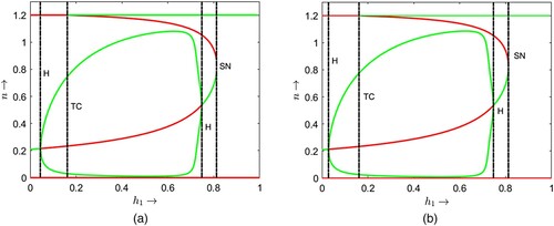
Figure 7. The bifurcation diagram with respect to the parameter $h_1$ with $\sigma =10$, $\kappa =1.2$, $\alpha =2.217$, $\text{β}=0.1$: (a) $\tau =0.0701$ and (b) $\tau =0.11$.

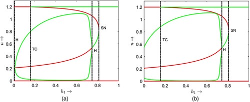
Figure 8. The bifurcation diagram with respect to the parameter $h_1$ with $\sigma =10$, $\kappa =1.2$, $\alpha =2.217$, $\tau =0.2$, $\text{β}=0.5$.

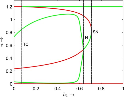
We can also check the bifurcation diagram with the time delay τ as bifurcation parameter (Figure 9). This bifurcation diagram shows that the coexistence of prey and their predator of the considered model system is only possible within a certain range of delay parameter magnitude. For a unique coexistence equilibrium point, a short maturation delay is required. For other fixed parameter values as in the caption of Figure 9, when the maturation time is substantially low then due to increment in the magnitude of the delay parameter the system starts to exhibit oscillatory coexistence after crossing the first Hopf bifurcation threshold ${\tau }_{H_1}=0.03$. The originated limit cycle through Hopf bifurcation is the only stable attractor of the system for ${\tau }_{H_1}<\tau <{\tau }_{\mathrm{TC}}$, where ${\tau }_{\mathrm{TC}}=0.138$ is the transcritical bifurcation threshold. This is due to initial negative feedback on the growth of predator population. There is a node-cycle bi-stability between the prey only equilibrium point $E_1$ and the locally stable limit cycle for ${\tau }_{\mathrm{TC}}<\tau <{\tau }_{H_2}$, where ${\tau }_{H_2}=0.98$ is the second Hopf bifurcation threshold through which the associated unstable positive equilibrium point becomes locally stable and remain stable until becomes infeasible through saddle-node bifurcation at ${\tau }_{\mathrm{SN}}=1.557$. 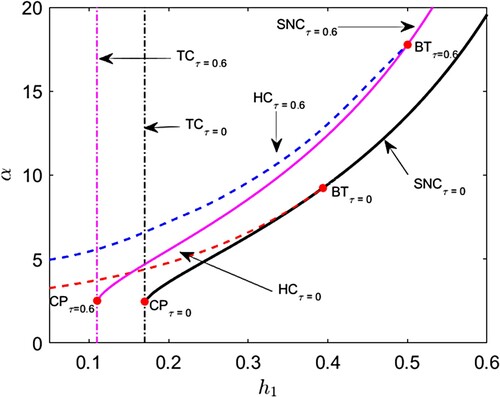We also attempt to comprehend the shift of bifurcation curves and corresponding co-dimension two bifurcations in the $h_1-\alpha$ parametric plane when maturation delay is included in the corresponding predator–prey model (Figure 10). It is observed when a permissible amount of maturation delay is allowed in the model system, then both the saddle-node bifurcation curve and the Hopf bifurcation curve shift to a left-upper position in $h_1-\alpha$ parametric domain. The transcritical bifurcation curve moves to left in the parametric domain if delay is incorporated. When delay is taken into account, the cusp bifurcation point, which is the meeting point of the saddle-node bifurcation curve and transcritical bifurcation, shifts from $(0.17,2.487)(\tau =0)$ to $(0.11,2.499)(\tau =0.6)$, i.e. moves to the left-upper position in the parametric plane. The Bogdanov–Takens bifurcation point, where the saddle-node bifurcation curve intersects the Hopf bifurcation curve, shifts from $(0.394,9.241)(\tau =0)$ to $(0.5,17.77)(\tau =0.6)$, i.e. moves to the right-upper of the $h_1-\alpha$ parametric domain.

Figure 9. The bifurcation diagram with respect to the parameter τ with $\sigma =10$, $\kappa =1.2$, $\alpha =2$, $h_1=0.1$, $\text{β}=0.5$.

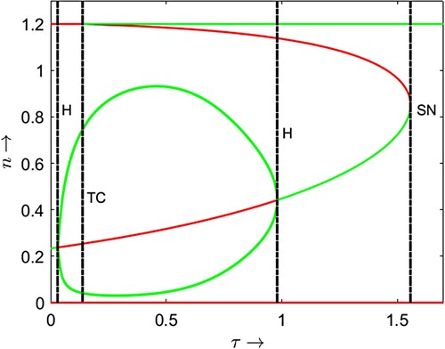
Figure 10. (Shift of bifurcation curves and bifurcation thresholds) $\sigma =0.4,\kappa =1.2,\text{ β}=0.1$. Black and magenta colour solid curves represent saddle node bifurcation curves (SNC) for $\tau =0$ and $\tau =0.6$ respectively. Red and blue colour broken curves represent Hopf bifurcation curves (HC) for $\tau =0$ and $\tau =0.6$ respectively. Black and magenta colour vertical dash–dot curves represent transcritical bifurcation curves for (TC) for $\tau =0$ and $\tau =0.6$ respectively. BT and CP stand for Bogdanov–Takens bifurcation threshold and cusp bifurcation thresholds respectively.

5. Discussion

In this article, we have studied the dynamics of prey–predator models incorporating hunting cooperation among predator species, for which a hunting time is considered in a predation term. In Section 2, for the model (2), when a hunting time $h_1$ is large (such that $\frac{\kappa }{1+h_1\kappa }\le 1$ holds), the number of coexistence equilibria is varied by the product of a cooperation rate and an intrinsic rate of growth of prey species $\mathrm{\alpha \sigma }$. Therefore, the introduction of hunting cooperation among predators emerges as a pivotal factor in shaping both the ecological equilibrium states (Figures 1 and 2) and thus the dynamical stability of the underlying system. By varying $h_1$, one can also observe a characteristic bifurcation dynamics including not only transcritical bifurcation at a predator-free equilibrium but also saddle-node bifurcation at a coexistence equilibrium for small α and saddle-node, Hopf bifurcation at a coexistence equilibrium for large α (see Figure 3). This suggests that, when cooperation among predator species is weak, prey species tend to evade extinction and instead coexist with predators, especially when the predators have sufficiently long hunting times. In Section 3, we have introduced the model (15) in which the maturation delay for predator species τ is incorporated. Even if $\frac{\kappa }{1+h_1\kappa }$ exceeds 1, a predator-free equilibrium is still asymptotically stable as long as it does not exceeds ${\mathrm{e}}^{\text{β}\tau }$. This implies that predator species tend to go extinct when τ is large because the long maturation delay suppresses the increment of the predation term for predator species. Figure 5 represents that a brief hunting time ($h_1$) suffices to trigger shifts in ecological coexistence when there is a substantial maturation delay (τ). Even with short hunting time, a large τ prompts transitions: from single stable state to double stable states and from double stable states to no coexistence stable state. As maturation delay (τ) increases, oscillations in population size initially intensify (large amplitude) at intermediate τ, showcasing a balance between predator-free and coexistence states. Subsequently, a state of bi-stability emerges between these points. However, with further τ values, coexistence collapses, leaving the predator-free equilibrium as the sole stable state. This implies that extended maturation delays can disrupt ecological balance, favouring a less diverse and stable state dominated by the predator-free equilibrium (see Figures 6, 7 and 8). It is worth noting from Figures 10 and 11 that reduced cooperation among predators results in intricate bifurcation dynamics when hunting time serves as the bifurcation parameter. This suggests that when predators lack cooperation in hunting, the population dynamics of predators and prey become highly sensitive to changes in hunting time, leading to unpredictable variations. From a biological point of view, such unforeseeable dynamics will arise from variation in behaviour of the predators for hunting due to the less cooperation effect. Further theoretical analysis on the bifurcation dynamics of the model (15) is our future work.

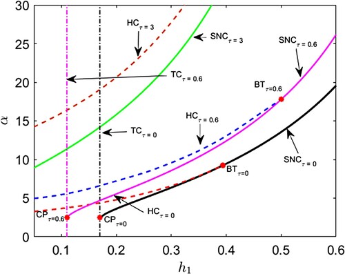
Figure 11. (Shift of bifurcation curves and bifurcation thresholds) $\sigma =0.4,\kappa =1.2,\text{ β}=0.1$. Black, magenta and green colour solid curves represent saddle node bifurcation curves (SNC) for $\tau =0$, $\tau =0.6$ and $\tau =3$ respectively. Red, blue and brown colour broken curves represent Hopf bifurcation curves (HC) for $\tau =0$, $\tau =0.6$ and $\tau =3$ respectively. Black and magenta colour vertical dash–dot curves represent transcritical bifurcation curves for (TC) for $\tau =0$ and $\tau =0.6$ respectively. BT and CP stand for Bogdanov–Takens bifurcation threshold and cusp bifurcation thresholds respectively.

Acknowledgements

The authors wish to express their gratitude to the editors and anonymous referees for helpful comments and valuable suggestion which improved the quality of this paper.

Disclosure statement

No potential conflict of interest was reported by the author(s).

Additional information

Funding

This research was partially supported by JSPS KAKENHI Grant Number 19K14598 (YE).

Appendices

Appendix 1.

Well-posedness

In this appendix, we prove the well-posedness of the model (2).

Proposition A.1

The model (2) is well-posed.

Proof.

The right-hand side of (2) is completely continuous and locally Lipschitzian on ${\mathbb{R}}_{+}^2$. It follows that the solution of (2) exists and is unique on $[0,T)$ for some $T>0$. One can obtain that $n\left(t\right)>0,p\left(t\right)>0$ for all $t\in [0,T)$. Furthermore, for $t\in [0,T)$, we obtain $\begin{array}{rl}\frac{\mathrm{d}}{\mathrm{d}t}\left(n\right(t)+p(t\left)\right)& =\mathrm{\sigma n}\left(t\right)(1-\frac{n\left(t\right)}{\kappa })-p\left(t\right)\\ & \le \sigma (\kappa -n(t\left)\right)-p\left(t\right)\\ & \le \mathrm{\sigma \kappa }-min\{\sigma ,1\}\left(n\right(t)+p(t\left)\right),\end{array}$which implies that $\left(n\right(t),p(t\left)\right)$ is uniformly bounded on $[0,T)$ by the positivity of $n\left(t\right)$ and $p\left(t\right)$ on $[0,T)$. Thus $T=\mathrm{\infty }$, that is, $\left(n\right(t),p(t\left)\right)$ exists and is unique and $n\left(t\right)>0,p\left(t\right)>0$ for all $t>0$. One can easily prove that the solution of (2) is continuous with respect to the initial values. This completes the proof.

Appendix 2.

Hopf bifurcation for $h_1=0$ for (2)

Assume that $\kappa >1$ holds. Substituting $h_1=0$ into (12(12) $\begin{array}{rl}\mathrm{tr}{J}_{+}& =\sigma (1-\frac{2n_{\ast }}{\kappa })-(1+\alpha p_{\ast })p_{\ast }(1-h_1{)}^2+\frac{\alpha p_{\ast }(1-h_1)}{1+\alpha p_{\ast }}\\ & =(1+\alpha p_{\ast })p_{\ast }(1-h_1)h_1-\sigma \frac{1}{\kappa (1-h_1)(1+\alpha p_{\ast })}+\frac{\alpha p_{\ast }(1-h_1)}{1+\alpha p_{\ast }}\end{array}$(12) ) and (13(13) $\begin{array}{rl}det{J}_{+}& =\sigma (1-\frac{2n_{\ast }}{\kappa })\frac{\alpha p_{\ast }(1-h_1)}{1+\alpha p_{\ast }}+p_{\ast }(1+\alpha p_{\ast })(1-h_1{)}^2\\ & =\left(p_{\ast }\right(1-h_1\left)\right(1+\alpha p_{\ast })-\sigma \frac{1}{\kappa (1-h_1)(1+\alpha p_{\ast })})\frac{\alpha p_{\ast }(1-h_1)}{1+\alpha p_{\ast }}\\ & +p_{\ast }(1+\alpha p_{\ast })(1-h_1{)}^2.\end{array}$(13) ), one can see that $\begin{array}{rl}\mathrm{tr}{J}_{+}& =-\sigma \frac{1}{\kappa (1+\alpha p_{\ast })}+\frac{\alpha p_{\ast }}{1+\alpha p_{\ast }}=\frac{\alpha p_{\ast }-\frac{\sigma }{\kappa }}{1+\alpha p_{\ast }},\\ det{J}_{+}& =\left(p_{\ast }\right(1+\alpha p_{\ast })-\sigma \frac{1}{\kappa (1+\alpha p_{\ast })})\frac{\alpha p_{\ast }}{1+\alpha p_{\ast }}+p_{\ast }(1+\alpha p_{\ast })\\ & =\frac{1}{1+\alpha p_{\ast }}(\left(p_{\ast }\right(1+\alpha p_{\ast }{)}^2-\frac{\sigma }{\kappa })\frac{\alpha p_{\ast }}{1+\alpha p_{\ast }}+p_{\ast }(1+\alpha p_{\ast }{)}^2)\\ & =\frac{\sigma }{1+\alpha p_{\ast }}((1-\frac{2}{\kappa }+\alpha p_{\ast })\frac{\alpha p_{\ast }}{1+\alpha p_{\ast }}+1-\frac{1}{\kappa }+\alpha p_{\ast }).\end{array}$It is noting that $\det J_{+}>0$ always holds true because $(1-\frac{2}{\kappa }+\alpha p_{\ast })\frac{\alpha p_{\ast }}{1+\alpha p_{\ast }}+1-\frac{1}{\kappa }+\alpha p_{\ast }>(1+2\alpha p_{\ast })(1-\frac{1}{\kappa })>0$. We have $\begin{array}{rl}(\mathrm{tr}{J}_{+}{)}^2-4det{J}_{+}& ={\left(\frac{\alpha p_{\ast }-\frac{\sigma }{\kappa }}{1+\alpha p_{\ast }}\right)}^2-4\left(p_{\ast }\right(1+\alpha p_{\ast })-\sigma \frac{1}{\kappa (1+\alpha p_{\ast })})\frac{\alpha p_{\ast }}{1+\alpha p_{\ast }}-4p_{\ast }(1+\alpha p_{\ast })\\ & =\frac{1}{(1+\alpha p_{\ast }{)}^2}({(\alpha p_{\ast }+\frac{\sigma }{\kappa })}^2-4\sigma (1-\frac{1}{\kappa }+\alpha p_{\ast })(1+2\alpha p_{\ast }\left)\right)\\ & =\frac{1}{(1+\alpha p_{\ast }{)}^2}\left(\right(1-8\sigma \left)\right(\alpha p_{\ast }{)}^2+\sigma (\frac{10}{\kappa }-12)\alpha p_{\ast }+\frac{\sigma }{{\kappa }^2}(\sigma -4\kappa (\kappa -1\left)\right)).\end{array}$Since $\begin{array}{rl}& \sigma (1-\frac{1}{\kappa })+(\mathrm{\alpha \sigma }-1)p_{\ast }-2\alpha (p_{\ast }{)}^2-{\alpha }^2(p_{\ast }{)}^3=0,\\ & \mathrm{i}.\mathrm{e}.\sigma (1-\frac{1}{\kappa })+\mathrm{\sigma \alpha }{p}_{\ast }=p_{\ast }(1+\alpha p_{\ast }{)}^2,\end{array}$$\alpha p_{\ast }\left(\alpha \right)$ is strictly monotone increasing on α. Due to the characteristic equation $det(J_{+}-\mathrm{\lambda I})={\lambda }^2-\left(\mathrm{tr}{J}_{+}\right)\lambda +det{J}_{+}=0$, if $\sigma >max\{\frac{1}{8},4{\kappa }^2-4\kappa \}$, then there exists a unique $\overline{\alpha }>0$ such that $(1-8\sigma )\left(\overline{\alpha }{p}_{\ast }\right(\overline{\alpha }){)}^2+\sigma (\frac{10}{\kappa }-12)\overline{\alpha }{p}_{\ast }(\overline{\alpha })+\frac{\sigma }{{\kappa }^2}(\sigma -4\kappa (\kappa -1))=0$and the following statement holds true:

1. If $0\le \alpha p_{\ast }<\frac{\sigma }{\kappa }$, it holds that $\mathrm{tr}{J}_{+}<0$.

2. If $\alpha p_{\ast }>\frac{\sigma }{\kappa }$, it holds that $\mathrm{tr}{J}_{+}>0$.

Therefore, if $\sigma >max\{\frac{1}{8},4{\kappa }^2-4\kappa \}$, then (2) undergoes Hopf bifurcation at $E=E_{+}$ when α crosses a critical value ${\alpha }_H$. Here ${\alpha }_H$ is a unique solution of ${\alpha }_H{p}_{\ast }\left({\alpha }_H\right)=\frac{\sigma }{\kappa }$.

Appendix 3.

Notations in Section 2.4.1

The notations used in Section 2.4.1 are as follows: $\begin{array}{rl}{a}_{10}& =n_{\ast }(-\frac{\sigma }{k}+\frac{{(\alpha p_{\ast }+1)}^2{p}_{\ast }{h}_1}{(n_{\ast }{p}_{\ast }\alpha h_1+h_1{n}_{\ast }+1)(1+h_1(\alpha p_{\ast }+1)n_{\ast })})+\sigma (1-\frac{n_{\ast }}{k})-\frac{(\alpha p_{\ast }+1)p_{\ast }}{1+h_1(\alpha p_{\ast }+1)n_{\ast }},\\ a_{01}& =-\frac{n_{\ast }}{n_{\ast }{p}_{\ast }\alpha h_1+h_1{n}_{\ast }+1}(2\alpha p_{\ast }+1-\frac{(\alpha p_{\ast }+1)p_{\ast }{h}_1\alpha n_{\ast }}{n_{\ast }{p}_{\ast }\alpha h_1+h_1{n}_{\ast }+1}),\\ a_{20}& =\frac{n_{\ast }(-{p_{\ast }}^3{\alpha }^2{h}_1-2{p_{\ast }}^2\alpha h_1-p_{\ast }{h}_1)h_1(\alpha p_{\ast }+1)}{{(n_{\ast }{p}_{\ast }\alpha h_1+h_1{n}_{\ast }+1)}^3}-\frac{\sigma }{k}+\frac{{(\alpha p_{\ast }+1)}^2{p}_{\ast }{h}_1}{{(n_{\ast }{p}_{\ast }\alpha h_1+h_1{n}_{\ast }+1)}^2},\\ a_{11}& =\frac{(-\alpha p_{\ast }-1)h_1{n}_{\ast }-2\alpha p_{\ast }-1}{{(1+h_1(\alpha p_{\ast }+1)n_{\ast })}^3},\\ a_{02}& =-\frac{n_{\ast }}{1+h_1(\alpha p_{\ast }+1)n_{\ast }}(\alpha -\frac{(n_{\ast }{p_{\ast }}^2{\alpha }^2{h}_1+2n_{\ast }{p}_{\ast }\alpha h_1+n_{\ast }{h}_1+2\alpha p_{\ast }+1)h_1\alpha n_{\ast }}{{(n_{\ast }{p}_{\ast }\alpha h_1+n_{\ast }{h}_1+1)}^2}),\\ a_{30}& =-\frac{n_{\ast }(-{p_{\ast }}^4{\alpha }^3{h_1}^2-3{p_{\ast }}^3{\alpha }^2{h_1}^2-3{p_{\ast }}^2\alpha {h_1}^2-p_{\ast }{h_1}^2)h_1(\alpha p_{\ast }+1)}{{(n_{\ast }{p}_{\ast }\alpha h_1+n_{\ast }{h}_1+1)}^3(1+h_1(\alpha p_{\ast }+1)n_{\ast })}+\frac{(-{p_{\ast }}^3{\alpha }^2{h}_1-2{p_{\ast }}^2\alpha h_1-p_{\ast }{h}_1)h_1(\alpha p_{\ast }+1)}{{(n_{\ast }{p}_{\ast }\alpha h_1+n_{\ast }{h}_1+1)}^2(1+h_1(\alpha p_{\ast }+1)n_{\ast })},\\ a_{21}& =\frac{(\alpha p_{\ast }+1)h_1(h(\alpha p_{\ast }+1)p_{\ast }+3\alpha p_{\ast }+1)}{{(1+h_1(\alpha p_{\ast }+1)p_{\ast })}^4},\\ a_{12}& =\frac{(-1+{h_1}^2(\alpha p_{\ast }+1){n_{\ast }}^2+2n_{\ast }{p}_{\ast }\alpha h_1)\alpha }{{(1+h_1(\alpha p_{\ast }+1)n_{\ast })}^4},\end{array}$ $\begin{array}{rl}{a}_{03}& =-\frac{(-n_{\ast }\alpha h_1-\alpha )h_1\alpha {n_{\ast }}^2}{{(n_{\ast }{p}_{\ast }\alpha h_1+n_{\ast }{h}_1+1)}^3(1+h_1(\alpha p_{\ast }+1)n_{\ast })},\\ b_{10}& =\frac{1}{1+h_1(\alpha p_{\ast }+1)n_{\ast }}((\alpha p_{\ast }+1)p_{\ast }-\frac{n_{\ast }{(\alpha p_{\ast }+1)}^2{p}_{\ast }{h}_1}{n_{\ast }{p}_{\ast }\alpha h_1+n_{\ast }{h}_1+1}),\\ b_{01}& =\frac{1}{1+h_1(\alpha p_{\ast }+1)n_{\ast }}(n_{\ast }(\alpha p_{\ast }+1)+n_{\ast }{p}_{\ast }\alpha -\frac{{n_{\ast }}^2(\alpha p_{\ast }+1)p_{\ast }{h}_1\alpha }{n_{\ast }{p}_{\ast }\alpha h_1+n_{\ast }{h}_1+1})-1,\\ b_{20}& =-\frac{({p_{\ast }}^2\alpha +p_{\ast })h_1(\alpha p_{\ast }+1)}{{(n_{\ast }{p}_{\ast }\alpha h_1+n_{\ast }{h}_1+1)}^2(1+h_1(\alpha p_{\ast }+1)n_{\ast })},\\ b_{11}& =\frac{n_{\ast }{p}_{\ast }\alpha h_1+n_{\ast }{h}_1+2\alpha p_{\ast }+1}{{(n_{\ast }{p}_{\ast }\alpha h_1+n_{\ast }{h}_1+1)}^3},\\ b_{02}& =\frac{n_{\ast }\alpha (n_{\ast }{h}_1+1)}{{(n_{\ast }{p}_{\ast }\alpha h_1+n_{\ast }{h}_1+1)}^3},\\ b_{30}& =-\frac{(-{p_{\ast }}^3{\alpha }^2{h}_1-2{p_{\ast }}^2\alpha h_1-p_{\ast }{h}_1)h_1(\alpha p_{\ast }+1)}{{(n_{\ast }{p}_{\ast }\alpha h_1+n_{\ast }{h}_1+1)}^3(1+h_1(\alpha p_{\ast }+1)n_{\ast })},\\ b_{21}& =-\frac{(\alpha p_{\ast }+1)h_1(h_1(\alpha p_{\ast }+1)n_{\ast }+3\alpha p_{\ast }+1)}{{(1+h_1(\alpha p_{\ast }+1)n_{\ast })}^4},\\ b_{12}& =-\frac{\alpha ({n_{\ast }}^2{p}_{\ast }\alpha {h_1}^2+{n_{\ast }}^2{h_1}^2+2n_{\ast }{p}_{\ast }\alpha h_1-1)}{{(n_{\ast }{p}_{\ast }\alpha h_1+n_{\ast }{h}_1+1)}^4},\\ b_{03}& =-\frac{({n_{\ast }}^2\alpha h_1+n_{\ast }\alpha )h_1\alpha n_{\ast }}{{(n_{\ast }{p}_{\ast }\alpha h_1+n_{\ast }{h}_1+1)}^3(1+h_1(\alpha p_{\ast }+1)n_{\ast })}.\end{array}$In addition, $A_1$ and $A_2$ are defined as follows: $\begin{array}{rl}{A}_1& =(a_{20}{a}_{01}^2-a_{11}{a}_{01}{a}_{10}+a_{02}{a}_{10}^2)X_1^2+h_{1_0}(2a_{02}{a}_{10}-a_{11}{a}_{01})X_1{X}_2+h_{1_0}^2{a}_{02}{X}_2^2\\ & +(a_{12}{a}_{01}{a}_{10}^2-a_{03}{a}_{10}^3+a_{30}{a}_{01}^3-a_{21}{a}_{01}^2{a}_{10})X_1^3+h_{1_0}(2a_{12}{a}_{10}{a}_{01}-a_{21}{a}_{01}^2-3a_{03}{a}_{10}^2)X_1^2{X}_2\\ & +h_{1_0}^2(a_{12}{a}_{01}-3a_{03}{a}_{10})X_1{X}_2^2-h_{1_0}{a}_{03}{X}_2^3,\\ A_2& =(b_{20}{a}_{01}^2-b_{11}{a}_{01}{a}_{10}+b_{02}{a}_{10}^2)X_1^2+h_{1_0}(2b_{02}{a}_{10}-b_{11}{a}_{01})X_1{X}_2+h_{1_0}^2{b}_{02}{X}_2^2\\ & +(b_{30}{a}_{01}^3+b_{12}{a}_{01}{a}_{10}^2-b_{21}{a}_{01}^2{a}_{10}-b_{03}{a}_{10}^3)X_1^3+h_{1_0}(2b_{12}{a}_{10}{a}_{01}-b_{21}{a}_{01}^2-3b_{03}{a}_{10}^2)X_1^2{X}_2\\ & +h_{1_0}^2(b_{12}{a}_{01}-3b_{03}{a}_{10})X_1{X}_2^2-h_{1_0}{b}_{03}{X}_2^3.\end{array}$

References

- Kot M. Elements of mathematical ecology. Cambridge: Cambridge University Press; 2001.
- Kuang Y, Freedman HI. Uniqueness of limit cycles in gause-type models of predator-prey systems. Math Biosci. 1988;88:67–84. doi: 10.1016/0025-5564(88)90049-1
- Přibylová L, Berec L. Predator interference and stability of predator–prey dynamics. J Math Biol. 2015;71:301–323. doi: 10.1007/s00285-014-0820-9
- Tyutyunov YV, Titova LI. From Lotka–Volterra to Arditi–Ginzburg: 90 years of evolving trophic functions. Biol Bull Rev. 2020;10:167–185. doi: 10.1134/S207908642003007X
- Arditi R, Ginzburg LR. Coupling in predator–prey dynamics: ratio-dependence. J Theor Biol. 1989;139:311–326. doi: 10.1016/S0022-5193(89)80211-5
- Cosner C, DeAngelis DL, Ault JS, et al. Effects of spatial grouping on the functional response of predators. Theor Popul Biol. 1999;56:65–75. doi: 10.1006/tpbi.1999.1414
- Holling CS. Some characteristics of simple types of predation and parasitism. Can Entomol. 1959;91:385–398. doi: 10.4039/Ent91385-7
- Kuang Y, Beretta E. Global qualitative analysis of a ratio-dependent predator–prey system. J Math Biol. 1998;36:389–406. doi: 10.1007/s002850050105
- Xiao D, Ruan S. Global dynamics of a ratio-dependent predator–prey system. J Math Biol. 2001;43:268–290. doi: 10.1007/s002850100097
- Bazykin AD. Nonlinear dynamics of interacting populations. Singapore: World Scientific; 1998.
- Lu M, Huang J. Global analysis in Bazykin's model with Holling II functional response and predator competition. J Differ Equ. 2021;280:99–138. doi: 10.1016/j.jde.2021.01.025
- Courchamp F, Berec L, Gascoigne J. Allee effects in ecology and conservation. Oxford: OUP Oxford; 2008.
- Stephens PA, Sutherland WJ, Freckleton RP. What is the Allee effect?. Oikos. 1999;87:185–190. doi: 10.2307/3547011
- Hilker FM. Population collapse to extinction: the catastrophic combination of parasitism and Allee effect. J Biol Dyn. 2010;4:86–101. doi: 10.1080/17513750903026429
- Morozov A, Petrovskii S, Li BL. Spatiotemporal complexity of patchy invasion in a predator–prey system with the Allee effect. J Theor Biol. 2006;238:18–35. doi: 10.1016/j.jtbi.2005.05.021
- Banerjee M, Takeuchi Y. Maturation delay for the predators can enhance stable coexistence for a class of prey–predator models. J Theor Biol. 2017;412:154–171. doi: 10.1016/j.jtbi.2016.10.016
- Sen M, Banerjee M, Morozov A. Bifurcation analysis of a ratio-dependent prey–predator model with the Allee effect. Ecol Complex. 2012;11:12–27. doi: 10.1016/j.ecocom.2012.01.002
- Erbach A, Lutscher F, Seo G. Bistability and limit cycles in generalist predator-prey dynamics. Ecol Complex. 2013;14:48–55. doi: 10.1016/j.ecocom.2013.02.005
- Sen D, Petrovskii S, Ghorai S, et al. Rich bifurcation structure of prey–predator model induced by the Allee effect in the growth of generalist predator. Int J Bifurcat Chaos. 2020;30:Article ID 2050084. doi: 10.1142/S0218127420500844
- Beddington JR. Mutual interference between parasites or predators and its effect on searching efficiency. J Anim Ecol. 1975;44:331–340. doi: 10.2307/3866
- Cantrell RS, Cosner C. On the dynamics of predator–prey models with the Beddington–DeAngelis functional response. J Math Anal Appl. 2001;257:206–222. doi: 10.1006/jmaa.2000.7343
- DeAngelis DL, Goldstein RA, O'Neill RV. A model for tropic interaction. Ecology. 1975; 56:881–892. doi: 10.2307/1936298
- Nilsson PA, Lundberg P, Brönmark C, et al. Behavioral interference and facilitation in the foraging cycle shape the functional response. Behav Ecol. 2007;18:354–357. doi: 10.1093/beheco/arl094
- Zhang Y, Richardson JS. Unidirectional prey–predator facilitation: apparent prey enhance predators' foraging success on cryptic prey. Biol Lett. 2007;3:348–351. doi: 10.1098/rsbl.2007.0087
- Berec L. Impacts of foraging facilitation among predators on predator–prey dynamics. Bull Math Biol. 2010;72:94–121. doi: 10.1007/s11538-009-9439-1
- Alves MT, Hilker FM. Hunting cooperation and Allee effects in predators. J Theor Biol. 2017;419:13–22. doi: 10.1016/j.jtbi.2017.02.002
- Beretta E, Kuang Y. Convergence results in a well-known delayed predator–prey system. J Math Anal Appl. 1996;204:840–853. doi: 10.1006/jmaa.1996.0471
- Kuang Y. Delay differential equations: with applications in population dynamics. Boston: Academic Press; 1993.
- MacDonald N. Time lags in biological models. Vol. 27. Springer Science & Business Media; 2013.
- Xiao Y, Chen L. Modeling and analysis of a predator–prey model with disease in the prey. Math Biosci. 2001;171:59–82. doi: 10.1016/S0025-5564(01)00049-9
- Cushing JM. Integrodifferential equations and delay models in population dynamics. Vol. 20. Springer Science & Business Media; 2013.
- Hadeler KP, Mackey MC, Stevens A. Topics in mathematical biology. Berlin: Springer; 2017.
- Ruan S. On nonlinear dynamics of predator-prey models with discrete delay. Math Model Nat Phenom. 2009;4:140–188. doi: 10.1051/mmnp/20094207
- Volterra V. Variations and fluctuations of the number of individuals in animal species living together. Anim Ecol. 1926;409–448.
- Mackey MC, Glass L. Oscillation and chaos in physiological control systems. Science. 1977;197:287–289. doi: 10.1126/science.267326
- Nakaoka S, Saito Y, Takeuchi Y. Stability, delay, and chaotic behavior in a Lotka–Volterra predator–prey system. Math Biosci Eng. 2006;3:173–187. doi: 10.3934/mbe.2006.3.173
- Tang S, Chen L. Global qualitative analysis for a ratio-dependent predator–prey model with delay. J Math Anal Appl. 2002;266:401–419. doi: 10.1006/jmaa.2001.7751
- Xiao D, Ruan S. Multiple bifurcations in a delayed predator–prey system with nonmonotonic functional response. J Differ Equ. 2001;176:494–510. doi: 10.1006/jdeq.2000.3982
- Turchin P. Complex population dynamics. Princeton University Press; 2013.
- Perko L. Differential equations and dynamical systems. New York: Springer-Verlag; 2000.
- Martin A, Ruan S. Predator–prey models with delay and prey harvesting. J Math Biol. 2001;43:247–267. doi: 10.1007/s002850100095
- Roy J, Banerjee M. Global stability of a predator-prey model with generalist predator. Appl Math Lett. 2023;142:Article ID 108659. doi: 10.1016/j.aml.2023.108659
- Sen M, Banerjee M, Morozov A. Stage-structured ratio-dependent predator-prey models revisited: when should the maturation lag result in systems' destabilization?. Ecol Complex. 2014;19:23–34. doi: 10.1016/j.ecocom.2014.02.001
- Wangersky PJ, Cunningham WJ. Time lag in prey–predator population models. Ecology. 1957;38:136–139. doi: 10.2307/1932137
- Gourley SA, Kuang Y. A stage structured predator–prey model and its dependence on maturation delay and death rate. J Math Biol. 2004;49:188–200. doi: 10.1007/s00285-004-0278-2
- Liu S, Beretta E. A stage-structured predator–prey model of Beddington–DeAngelis type. SIAM J Appl Math. 2006;66:1101–1129. doi: 10.1137/050630003
- Liu S, Chen L, Liu Z. Extinction and permanence in nonautonomous competitive system with stage structure. J Math Anal Appl. 2002;274:667–684. doi: 10.1016/S0022-247X(02)00329-3