A risk-induced dispersal strategy of the infected population for a disease-free state in the SIS epidemic model

Abstract

This article proposes a dispersal strategy for infected individuals in a spatial susceptible-infected-susceptible (SIS) epidemic model. The presence of spatial heterogeneity and the movement of individuals play crucial roles in determining the persistence and eradication of infectious diseases. To capture these dynamics, we introduce a moving strategy called risk-induced dispersal (RID) for infected individuals in a continuous-time patch model of the SIS epidemic. First, we establish a continuous-time n-patch model and verify that the RID strategy is an effective approach for attaining a disease-free state. This is substantiated through simulations conducted on 7-patch models and analytical results derived from 2-patch models. Second, we extend our analysis by adapting the patch model into a diffusive epidemic model. This extension allows us to explore further the impact of the RID movement strategy on disease transmission and control. We validate our results through simulations, which provide the effects of the RID dispersal strategy.

Keywords:

• Spatial SIS model
• risk-induced dispersal
• continuous-time patch model
• diffusive epidemic model
• disease-free state

AMS Classification::

• 34D20
• 35K57
• 92D30
• 92B05

1. Introduction

In recent years, significant research efforts have been dedicated to interpreting the dynamics and mechanisms of infectious diseases. This understanding has been pursued through a variety of epidemic models based on differential equations, each offering distinct perspectives on the processes and outcomes of disease spread and control. The spatial heterogeneity of the environment, alongside the mobility rates of susceptible and infected individuals, are acknowledged as pivotal elements in understanding the persistence and eventual eradication of diseases. Depending on the heterogeneity and connectivity of the spatial environment, the mobility of individuals can either foster or obstruct the spread of a disease. This notion has been corroborated by studies such as those by Allen et al. [1–3], Bolker and Grenfell [4], Castillo and Yakubu [5,6], Hess [7], Lloyd and May [8], Ruan [9], and Salmani and Van [10], which underscore the necessity of integrating spatial parameters into epidemic modeling. Specifically, patch models and reaction-diffusion models have gained attention due to their ability to incorporate spatial heterogeneity in the environment and the movement rates of susceptible and infected individuals. Patch models [1,3,11–13,31,32] consider the population dynamics within discrete patches or compartments, allowing for the examination of spatial heterogeneity and connectivity. Reaction–diffusion models [2,9,14,15] describe the spread of the disease in continuous space, considering the diffusion of individuals between different locations.

To examine the influence of the heterogeneity of an environment and the movement of individuals on the persistence and extinction of a disease, SIS models were used in both continuous/discrete patch models [1,3,16] and reaction-diffusion models [2,17–20].

In [1,3], Allen et al. introduced a continuous and discrete n-patch model that incorporated the spatial heterogeneity of environments. They showed that without movement between patches, diseases persist exclusively in high-risk areas where the patch reproduction number exceeds one. This implies that diseases can establish and sustain themselves in regions where the infection risk is particularly high. However, when susceptible and infected individuals can move between patches, endemic equilibrium (EE) can emerge across all patches. In such a case, the disease can sustain itself across multiple regions simultaneously, signifying a stable coexistence of infected and susceptible individuals throughout different areas of the environment. For the case when n = 2, if only the infected individuals are allowed to move between the two patches, the high-risk patch becomes empty, and all susceptible individuals eventually reside in the low-risk patch, where the patch reproduction number is less than one. In recent research, specifically referenced in [16,21], the results presented in [1] have been expanded upon. These studies focus on systems with asymmetric connectivity between patches. Furthermore, the authors have addressed and resolved several open questions that were initially posited in [1].

For the partial differential equation model, many researchers considered the models with the ratio-dependent type infection mechanism having spatial heterogeneity. Allen et al. [2] proposed the model and showed the global stability of disease-free equilibrium (DFE) and the uniqueness of the endemic state; Peng and Liu [18] showed the global stability of the endemic state. Kuto et al. [17] and Cui et al. [22] showed some results for the reaction-diffusion-advection SIS model. Models with a logistic source and a model with a media coverage impact were discussed by Li et al. [23] and Ge et al. [24], respectively. Additionally, a model with a mass action-type infection mechanism was studied by Wen et al. [25].

In the context of disease control, the studies conducted by Allen et al. [1,2] and the subsequent studies [16,21] highlight the importance of a dispersal strategy for infected individuals in controlling the spread of infectious diseases. Their research focuses on models with constant diffusion rates for individuals' movement. In these models, the spatial domain is categorized as either low-risk or high-risk based on a comparison between the average patch transmission rates and the average recovery rates. Similarly, individual patches are deemed low-risk or high-risk depending on whether the patch transmission rate is lower or higher than the patch recovery rate, respectively. This classification corresponds to determining whether the patch reproduction number falls below or exceeds 1. One of the key results obtained in these studies is the definition of a basic reproduction number ($R_0$) based on the movement rate of infected individuals incorporating the spatial heterogeneity of the environment. The existence of a unique disease-free equilibrium (DFE) and the dynamics of the system are then analyzed based on the value of $R_0$. Specifically, it is shown that if $R_0<1$, the DFE is globally asymptotically stable, indicating the potential for disease control. On the other hand, if $R_0>1$, a unique endemic equilibrium (EE) exists, suggesting that the disease persists in the population. These findings emphasize the critical role of dispersal strategies and the impact of spatial heterogeneity in disease control. By understanding the relationship between transmission rates, recovery rates, and the movement of infected individuals, effective control measures can be developed to achieve disease eradication or containment.

The main objective of this study is to explore the potential of a nonuniform movement strategy for infected individuals, referred to as risk-induced dispersal (RID), as a means to improve disease control and achieve a disease-free state. The RID strategy is based on the idea that the rate of movement of infected individuals should be influenced by the environmental risk associated with disease transmission and recovery rates, taking into account the spatial heterogeneity of the region. More precisely, in the RID strategy, infected individuals are posited to move more rapidly within high-risk patches or domains – areas characterized by elevated disease transmission risks – compared to low-risk patches or domains, where the risk is substantially reduced. Notably, even within this framework, the movement rate of infected individuals remains slower than that of susceptible individuals. By incorporating this nonuniform movement strategy into our disease model, the study aims to assess its impact on disease dynamics and its efficacy in facilitating a disease-free state. The motivation behind this research is to explore innovative strategies that can enhance disease control efforts. By considering the influence of environmental risk on the movement of infected individuals, the RID strategy offers a promising approach to improving disease control measures and potentially reducing the overall prevalence of the disease.

The rest of this paper is structured as follows: In Section 2, we introduce n-patch models incorporating the RID strategy. We demonstrate that RID serves as an effective movement strategy for attaining a disease-free state. This is substantiated through simulations performed on 7-patch models and analytical results generated from 2-patch models. Section 3 expands the patch model into a diffusive epidemic model to elucidate the influence of this dispersal strategy. Finally, we summarize our results and discuss potential future research directions in Section 4.

2. Model description for the patch model

2.1. Risk-induced dispersal

We consider the following n-patch SIS model with RID: (1) $\{\begin{array}{l}\frac{\mathrm{d}{S}_i}{\mathrm{d}t}=I_i(-\frac{{\beta }_i{S}_i}{S_i+I_i}+r_i)-\sum _{j\ne i}^n{a}_{\mathrm{ij}}{S}_i+\sum _{j\ne i}^n{a}_{\mathrm{ji}}{S}_j\\ \frac{\mathrm{d}{I}_i}{\mathrm{d}t}=I_i(\frac{{\beta }_i{S}_i}{S_i+I_i}-r_i)-\sum _{j\ne i}^n{b}_{\mathrm{ij}}{I}_i+\sum _{j\ne i}^n{b}_{\mathrm{ji}}{I}_j\\ S_i(0)\ge 0,I_i(0)\ge 0,\end{array}$(1) where $S_i(t)$ and $I_i(t)$ denote the number of susceptible and infected individuals in patch $i\in \{1,\dots ,n\}$ at time $t\in {\mathbb{R}}^{+}$. $a_{\mathrm{ij}}$ and $b_{\mathrm{ij}}$ are positive coefficients that represent the movement rates of the susceptible and infected subpopulations, respectively, from patch i to patch j. ${\beta }_i$ and $r_i$ are the positive constants that express the rates of disease transmission and recovery in patch i. Here, we assume that $a_{\mathrm{ij}}=a_{\mathrm{ji}}$.

For each patch, we can define a patch-basic reproduction number ${\mathcal{R}}_0^i$ for i-patch by ${\mathcal{R}}_0^i={\beta }_i/r_i.$When there is no movement between patches, ${\mathcal{R}}_0^i$ is a basic reproduction number of the model with a ratio-dependent type infection. Therefore, we term a patch where the disease transmission rate is lower than the disease recovery rate a low-risk patch $({\mathcal{R}}_0^i<1)$. A high-risk patch is defined as the opposite.

Furthermore, we say that susceptible and infective individuals are in a low-risk domain(high-risk domain) if $\sum _{i=1}^n{\beta }_i/\sum _{i=1}^n{r}_i<(>)1.$To represent RID with infected individuals in our model, we give a movement rate $b_{\mathrm{ij}}$ as $b_{\mathrm{ij}}=\delta ({\mathcal{R}}_0^i),$where δ is an increasing function. This indicates the strategy of the infected individuals such that they move fast in the high-risk patch and slowly in the low-risk patch, i.e. the higher patch reproduction number is, the faster the infected individuals move. Here, δ can be chosen suitable for each constructed model.

It is noteworthy that since $b_{\mathrm{ij}}$ is defined as above, the connectivity matrix is not symmetric. We denote $a_{\mathrm{ij}}=d_S,b_{\mathrm{ij}}=d_I\delta ({\mathcal{R}}_0^i).$Then, (1(1) $\{\begin{array}{l}\frac{\mathrm{d}{S}_i}{\mathrm{d}t}=I_i(-\frac{{\beta }_i{S}_i}{S_i+I_i}+r_i)-\sum _{j\ne i}^n{a}_{\mathrm{ij}}{S}_i+\sum _{j\ne i}^n{a}_{\mathrm{ji}}{S}_j\\ \frac{\mathrm{d}{I}_i}{\mathrm{d}t}=I_i(\frac{{\beta }_i{S}_i}{S_i+I_i}-r_i)-\sum _{j\ne i}^n{b}_{\mathrm{ij}}{I}_i+\sum _{j\ne i}^n{b}_{\mathrm{ji}}{I}_j\\ S_i(0)\ge 0,I_i(0)\ge 0,\end{array}$(1) ) may be written as (2) $\{\begin{array}{l}\frac{\mathrm{d}{S}_i}{\mathrm{d}t}=I_i(-\frac{{\beta }_i{S}_i}{S_i+I_i}+r_i)-\sum _{j\ne i}^n{d}_S{S}_i+\sum _{j\ne i}^n{d}_S{S}_j\\ \frac{\mathrm{d}{I}_i}{\mathrm{d}t}=I_i(\frac{{\beta }_i{S}_i}{S_i+I_i}-r_i)-(n-1)d_I\delta ({\mathcal{R}}_0^i)I_i+\sum _{j\ne i}^n{d}_I\delta ({\mathcal{R}}_0^j)I_j\\ S_i(0)\ge 0,I_i(0)\ge 0.\end{array}$(2) Because of the asymmetry of the connectivity matrix, we only give mathematical results for the two-patch model in the next subsection. Instead, we introduce a numerical simulation of the effect of RID when the environment is a high-risk domain for n = 7. We use the following parameter: $\begin{array}{rl}& {\beta }_1=0.05,r_1=0.02,{\beta }_2=0.02,r_2=0.07,{\beta }_3=0.08,r_3=0.01,\\ & {\beta }_4=0.03,r_4=0.04,{\beta }_5=0.02,r_5=0.04,{\beta }_6=0.06,r_6=0.03,\\ & {\beta }_7=0.03,r_7=0.06,d_S=0.1,S_i(0)=0.5,I_i(0)=\mathrm{0.1.}\end{array}$Here, we consider the RID strategy with δ as a linear function $\delta ({\mathcal{R}}_0^i)=d_I{\mathcal{R}}_0^i$

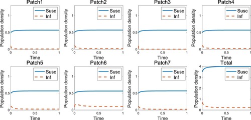
Figure 1 represents the endemic that occurs when the infected individuals move uniformly, which is the case when $\delta \equiv d_I$ as in the result of [1] that the endemic occurs in the high-risk domain. However, the disease-free state occurs if the infected individuals move according to the RID strategy (Figure 2). An appropriate speed of RID ($d_2=0.04$ in Figure 2) can change the endemic state to disease vanishing, but the disease does not disappear if the infected individual moves to other patches too slowly (Figure 3). When people get the infectious disease, the infected people barely move to other patches because they are sick. However, Figures 2 and 3 indicate that for the disease-free state, they should try to move faster than a certain speed (still slower than not infected people) to other patches, which helps the infected people reach low-risk patches in which people can easily recover. In the context of disease control, the concept of RID involves strategically relocating infected individuals from vulnerable areas to those with more robust medical systems, presenting a viable approach for managing infectious diseases. For readers interested in exploring this further, [26] provides a related perspective, illustrating the impact of human movement strategies on disease control within a spatial model of vector-borne diseases. However, from a border control standpoint, the increased movement of infectious individuals from high-risk to low-risk regions might not be feasible or politically acceptable. As noted in [13], a more commonly favored approach in managing such scenarios could involve restricting travel from high-risk to low-risk areas, reflecting the complexities and varied strategies in disease management and public policy.

Figure 1. Endemic occurs when the infected individuals without RID are in the high-risk domain ($d_I=0.05$).

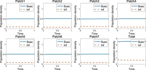
Figure 2. Disease-free occurs when the infected individuals move with RID in the high-risk domain ($d_I=0.05$).

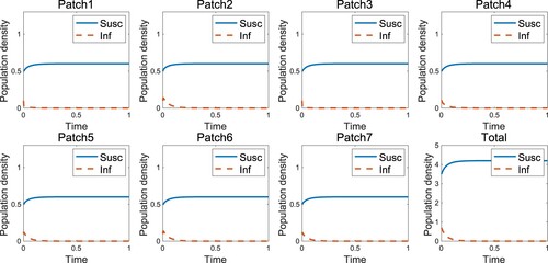
Figure 3. Endemic occurs when the infected individuals move with RID in the high-risk domain ($d_I=0.01$).

2.2. Mathematical approach for the 2-patch model

In this subsection, we provide a mathematical approach for the 2-patch model: (3) $\{\begin{array}{l}\frac{\mathrm{d}{S}_1}{\mathrm{d}t}=I_1(-\frac{{\beta }_1{S}_1}{S_1+I_1}+r_1)-d_S(S_1-S_2)\\ \frac{\mathrm{d}{I}_1}{\mathrm{d}t}=I_1(\frac{{\beta }_1{S}_1}{S_1+I_1}-r_1)-d_I(k{I}_1-I_2)\\ \frac{\mathrm{d}{S}_2}{\mathrm{d}t}=I_2(-\frac{{\beta }_2{S}_2}{S_2+I_2}+r_2)+d_S(S_1-S_2)\\ \frac{\mathrm{d}{I}_2}{\mathrm{d}t}=I_2(\frac{{\beta }_2{S}_2}{S_2+I_2}-r_2)+d_I(k{I}_1-I_2)\\ S_1(0)\ge 0,S_2(0)\ge 0,I_1(0)\ge 0,I_2(0)\ge 0,\end{array}$(3) Throughout this section, we assume that patch 1 is a high-risk patch and patch 2 is a low-risk patch, i.e. (A1) ${\beta }_1>r_1\text{and}{\beta }_2<r_2,$(A1) Here, $k\ge 1$. k = 1 is the case when the infected individuals move without RID, and k>1 indicates the strategy of the infected individuals such that they move fast in the high-risk patch and slowly in the low-risk patch.

We shall show ${\mathcal{R}}_0(1)>{\mathcal{R}}_0(k)$ for k>1, i.e. RID is an efficient strategy to obtain the disease-free state. Before starting, we let the initial total population N be given by $N=\sum _{i=1}^2[S_i(0)+I_i(0)]>0.$By adding the equations in (1(1) $\{\begin{array}{l}\frac{\mathrm{d}{S}_i}{\mathrm{d}t}=I_i(-\frac{{\beta }_i{S}_i}{S_i+I_i}+r_i)-\sum _{j\ne i}^n{a}_{\mathrm{ij}}{S}_i+\sum _{j\ne i}^n{a}_{\mathrm{ji}}{S}_j\\ \frac{\mathrm{d}{I}_i}{\mathrm{d}t}=I_i(\frac{{\beta }_i{S}_i}{S_i+I_i}-r_i)-\sum _{j\ne i}^n{b}_{\mathrm{ij}}{I}_i+\sum _{j\ne i}^n{b}_{\mathrm{ji}}{I}_j\\ S_i(0)\ge 0,I_i(0)\ge 0,\end{array}$(1) ), we obtain (4) $N=\sum _{i=1}^2[S_i(t)+I_i(t)]\text{for}t\ge 0,$(4) For $k\ge 1$, we first introduce some well-known results for (3(3) $\{\begin{array}{l}\frac{\mathrm{d}{S}_1}{\mathrm{d}t}=I_1(-\frac{{\beta }_1{S}_1}{S_1+I_1}+r_1)-d_S(S_1-S_2)\\ \frac{\mathrm{d}{I}_1}{\mathrm{d}t}=I_1(\frac{{\beta }_1{S}_1}{S_1+I_1}-r_1)-d_I(k{I}_1-I_2)\\ \frac{\mathrm{d}{S}_2}{\mathrm{d}t}=I_2(-\frac{{\beta }_2{S}_2}{S_2+I_2}+r_2)+d_S(S_1-S_2)\\ \frac{\mathrm{d}{I}_2}{\mathrm{d}t}=I_2(\frac{{\beta }_2{S}_2}{S_2+I_2}-r_2)+d_I(k{I}_1-I_2)\\ S_1(0)\ge 0,S_2(0)\ge 0,I_1(0)\ge 0,I_2(0)\ge 0,\end{array}$(3) ).

Lemma 2.1

Let N be fixed. Then, there exists a unique DFE $(\hat{S},0)$ given by ${\hat{S}}_i=N/2$ for $i\in \{1,2\}$.

From Lemma 2.1, we can obtain the basic reproduction number ${\mathcal{R}}_0(k)$ for (3(3) $\{\begin{array}{l}\frac{\mathrm{d}{S}_1}{\mathrm{d}t}=I_1(-\frac{{\beta }_1{S}_1}{S_1+I_1}+r_1)-d_S(S_1-S_2)\\ \frac{\mathrm{d}{I}_1}{\mathrm{d}t}=I_1(\frac{{\beta }_1{S}_1}{S_1+I_1}-r_1)-d_I(k{I}_1-I_2)\\ \frac{\mathrm{d}{S}_2}{\mathrm{d}t}=I_2(-\frac{{\beta }_2{S}_2}{S_2+I_2}+r_2)+d_S(S_1-S_2)\\ \frac{\mathrm{d}{I}_2}{\mathrm{d}t}=I_2(\frac{{\beta }_2{S}_2}{S_2+I_2}-r_2)+d_I(k{I}_1-I_2)\\ S_1(0)\ge 0,S_2(0)\ge 0,I_1(0)\ge 0,I_2(0)\ge 0,\end{array}$(3) ) using the next generation approach (see [27]):

Lemma 2.2

The basic reproduction number for (3(3) $\{\begin{array}{l}\frac{\mathrm{d}{S}_1}{\mathrm{d}t}=I_1(-\frac{{\beta }_1{S}_1}{S_1+I_1}+r_1)-d_S(S_1-S_2)\\ \frac{\mathrm{d}{I}_1}{\mathrm{d}t}=I_1(\frac{{\beta }_1{S}_1}{S_1+I_1}-r_1)-d_I(k{I}_1-I_2)\\ \frac{\mathrm{d}{S}_2}{\mathrm{d}t}=I_2(-\frac{{\beta }_2{S}_2}{S_2+I_2}+r_2)+d_S(S_1-S_2)\\ \frac{\mathrm{d}{I}_2}{\mathrm{d}t}=I_2(\frac{{\beta }_2{S}_2}{S_2+I_2}-r_2)+d_I(k{I}_1-I_2)\\ S_1(0)\ge 0,S_2(0)\ge 0,I_1(0)\ge 0,I_2(0)\ge 0,\end{array}$(3) ) is the spectral radius of the next generation matrix given by ${\mathcal{R}}_0(k)=\rho (F{V}^{-1}),$where $F=\mathrm{diag}({\beta }_i)\text{and}V=\left(\begin{array}{cc}{r}_1+k{d}_I& -d_I\\ -k{d}_I& r_2+d_I\end{array}\right).$

From the latter, we obtain the following lemma.

Lemma 2.3

Let the total population N be fixed, and let ${\lambda }_1$ be the largest eigenvalue of $(F-V)$. Then ${\lambda }_1$ is positive(negative) if and only if ${\mathcal{R}}_0(k)>1(<1)$.

Here are the properties of such eigenvalues.

Lemma 2.4

Let ${\lambda }_1$ be the largest eigenvalue of the matrix $(F-V)$. Then, ${\lambda }_1$ is strictly decreasing with respect to $d_I$ and $k\ge 1$.

Proof.

It follows from [28–30] that ${\lambda }_1$ is strictly decreasing for $d_I$. Thus, we only need to show that ${\lambda }_1$ is strictly decreasing for $k\ge 1$. Let L: = F−V. Then, $L-\mathrm{\lambda I}=\left(\begin{array}{cc}{\beta }_1-r_1-k{d}_I-\lambda & -d_I\\ -k{d}_I& {\beta }_2-r_2-d_I-\lambda \end{array}\right).$Hence, the characteristic equation is ${\lambda }^2-(A+B)\lambda +\mathrm{AB}-k{d}_I^2=0,$where $A={\beta }_1-r_1-k{d}_I$ and $B={\beta }_2-r_2-d_I$. Since $(A+B{)}^2-4(\mathrm{AB}-k{d}_I^2)=(A-B{)}^2+4k{d}_I^2\ge 0$, the eigenvalues of L are real. Therefore, ${\lambda }_1$ can be written as ${\lambda }_1=\frac{({\beta }_1+{\beta }_2-r_1-r_2)-(k+1)d_I+\sqrt{(({\beta }_1-{\beta }_2-r_1+r_2)+(1-k)d_I{)}^2+4k{d}_I^2}}{2}.$The derivative of ${\lambda }_1$ with respect to k, denoted $({\lambda }_1^{\prime }{)}_k$, is $\begin{array}{rl}({\lambda }_1^{\prime }{)}_k& =\frac{-d_I\sqrt{(C+(1-k)d_I{)}^2+4k{d}_I^2}-d_I(C+(1-k)d_I)+2d_I^2}{2\sqrt{(C+(1-k)d_I{)}^2+4k{d}_I^2}}\\ & =d_I\frac{-\sqrt{C^2-2C(k-1)d_I+(1+k{)}^2{d}_I^2}-C+(k+1)d_I}{2\sqrt{(C+(1-k)d_I{)}^2+4k{d}_I^2}}\\ & =d_I\frac{(-C+(k+1)d_I{)}^2-(C^2-2C(k-1)d_I+(1+k{)}^2{d}_I^2)}{\begin{array}{c}2\sqrt{(C+(1-k)d_I{)}^2+4k{d}_I^2}\\ (-C+(k+1)d_I+\sqrt{C^2-2C(k-1)d_I+(1+k{)}^2{d}_I^2})\end{array}}\\ & =d_I\frac{-4C{d}_I}{\begin{array}{c}2\sqrt{(C+(1-k)d_I{)}^2+4k{d}_I^2}\\ (-C+(k+1)d_I+\sqrt{C^2-2C(k-1)d_I+(1+k{)}^2{d}_I^2})\end{array}}\\ & <0,\end{array}$where $C={\beta }_1-{\beta }_2-r_1+r_2$, which is positive by assumption (A1). Since $C^2-2C(k-1)d_I+(1+k{)}^2{d}_I^2=[-C+(k+1)d_I{]}^2+4C{d}_I$, the last inequality holds. Therefore, ${\lambda }_1$ is strictly decreasing for $k\ge 1$.

As such, we provide the properties of ${\mathcal{R}}_0(k,d_I)$, denoting ${\mathcal{R}}_0(k)$ at $d_I$.

Theorem 2.5

Let ${\mathcal{R}}_0(k,d_I)$ be the basic reproduction number in Lemma 2.2. Then, ${\mathcal{R}}_0(k,d_I)$ is strictly decreasing in $d_I$. Moreover, if ${\mathcal{R}}_0(1)=1$, then ${\mathcal{R}}_0(k)<1$ for k>1.

Proof.

First, the strict monotonicity in $d_I$ follows from [21]. Suppose that ${\mathcal{R}}_0(1,d_I)=1$. Denoting ${\lambda }_1$ by ${\lambda }_1(k,d_I)$, we have ${\lambda }_1(1,d_I)=0$. Then Lemma 2.4 implies that ${\lambda }_1(k,d_I)<0$ for k>1, and thus ${\mathcal{R}}_0(k,d_I)<0$ for k>1 by Lemma 2.3.

Thus, we obtained the condition for the basic reproduction number ${\mathcal{R}}_0$, which covers the result in [1, Theorem 1].

Theorem 2.6

(i)	Suppose that the population is in a low-risk domain. For a given $k\ge 1$, there exists a threshold value $d_I^{\ast }(k)>0$ such that ${\mathcal{R}}_0(k)>1$ for $d_I<d_I^{\ast }(k)$ and ${\mathcal{R}}_0(k)<1$ for $d_I>d_I^{\ast }(k)$. Moreover, $d_I^{\ast }(k)<d_I^{\ast }(1)$ for k>1.
(ii)	Suppose that the population is in a high-risk domain. For a given $d_I$, there exists $k^{\ast }>1$ depending on $d_I,{\beta }_i$ and $r_i$ such that if $k>k^{\ast }$ then ${\mathcal{R}}_0(k)<1$, and if $k<k^{\ast }$ then ${\mathcal{R}}_0(k)>1$.

Proof.

(i) Suppose that the population is in a low-risk domain, which means ${\beta }_1+{\beta }_2-r_1-r_2<0$. From [1, Theorem 1], there exists $d_I^{\ast }(1)$ such that ${\mathcal{R}}_0(1,d_I^{\ast }(1))=1$, and thus from Theorem 2.5, ${\mathcal{R}}_0(k,d_I^{\ast }(1))<1$ for a given k>1, which is equivalent to ${\lambda }_1(k,d_I^{\ast }(1))<0$. Note that ${\lambda }_1=\frac{({\beta }_1+{\beta }_2-r_1-r_2)-(k+1)d_I+\sqrt{(({\beta }_1-{\beta }_2-r_1+r_2)+(1-k)d_I{)}^2+4k{d}_I^2}}{2}.$It can be easily checked that ${\lambda }_1(k,d_I)\to {\beta }_1-r_1>0$ as $d_I\to 0$. By the monotonicity of ${\lambda }_1$ for $d_I$, there exists $d_I^{\ast }(k)<d_I^{\ast }(1)$ such that ${\lambda }_1(k,d_I^{\ast }(k))=0$. Hence, ${\mathcal{R}}_0(k,d_I^{\ast }(k))=1$; as such, our assertion holds.

(ii) Suppose that the population is in a high-risk domain, i.e. ${\beta }_1+{\beta }_2-r_1-r_2>0$. We know that ${\mathcal{R}}_0(1)>1$ for all $d_I$ and ${\lambda }_1$ is strictly decreasing for $k\ge 1$ by Lemma 2.4. Let $A={\beta }_1+{\beta }_2-r_1-r_2$ and $B={\beta }_1-{\beta }_2-r_1+r_2$. Note that both A and B are independent of k. Therefore, $\begin{array}{rl}\underset{k\to \mathrm{\infty }}{lim}{\lambda }_1& =\underset{k\to \mathrm{\infty }}{lim}\frac{A-(k+1)d_I+\sqrt{(B+(1-k)d_I{)}^2+4k{d}_I^2}}{2}\\ & =\underset{k\to \mathrm{\infty }}{lim}\frac{(B+(1-k)d_I{)}^2+4k{d}_I^2-((k+1)d_I-A{)}^2}{2(\sqrt{(B+(1-k)d_I{)}^2+4k{d}_I^2}+((k+1)d_I-A))}\\ & =\underset{k\to \mathrm{\infty }}{lim}\frac{(B-A+2d_I)(B+A-2k{d}_I)+4k{d}_I^2}{2(\sqrt{(B+(1-k)d_I{)}^2+4k{d}_I^2}+((k+1)d_I-A))}\\ & =\underset{k\to \mathrm{\infty }}{lim}\frac{-2(B-A)k{d}_I+(B+A)(B-A+2d_I)}{2(\sqrt{(B+(1-k)d_I{)}^2+4k{d}_I^2}+((k+1)d_I-A))}\\ & =-(B-A)/2<0,\end{array}$because $B-A=2(r_2-{\beta }_2)>0$ by (A1). Thus, we can obtain $k^{\ast }>1$ such that ${\lambda }_1(k^{\ast })=0$. From the monotonicity, it follows that if $k>k^{\ast }$, then ${\lambda }_1(k)<0$, and conversely, if $k<k^{\ast }$, then ${\lambda }_1(k)>0$. Hence, the proof is conclusively established, drawing upon Lemma 2.3.

It's noteworthy that from the proof of Lemma 2.4, we observe that ${\lambda }_1$ decreases with k in the interval $(0,1)$. Consequently, we can deduce that $\underset{k\to 0}{lim}{\lambda }_1={\beta }_1-r_1>0$, which implies that ${\mathcal{R}}_0(k)>1$. This suggests that for k<1, there's a likelihood of the disease persisting within the domain. Particularly, it is anticipated that the disease may remain confined only to the high-risk patch in scenarios where infectious individuals in such patches are either locked down or restricted from travel ($k\ll 1$). We present this as a conjecture and leave its further exploration to interested readers.

Now, we show the result for the global stability of the DFE when ${\mathcal{R}}_0(k)<1$ and for EE when ${\mathcal{R}}_0(k)>1$. This can be shown in a similar way to [1], so we omit the proof here.

Lemma 2.7

Let the total population N be fixed. Then, the DFE is globally asymptotically stable for ${\mathcal{R}}_0(k)<1$.

Now, we show that EE exists when ${\mathcal{R}}_0(k)>1$. We consider the equation (5) $\{\begin{array}{l}0=I_1(-\frac{{\beta }_1{S}_1}{S_1+I_1}+r_1)-d_S(S_1-S_2)\\ 0=I_1(\frac{{\beta }_1{S}_1}{S_1+I_1}-r_1)-d_I(k{I}_1-I_2)\\ 0=I_2(-\frac{{\beta }_2{S}_2}{S_2+I_2}+r_2)+d_S(S_1-S_2)\\ 0=I_2(\frac{{\beta }_2{S}_2}{S_2+I_2}-r_2)+d_I(k{I}_1-I_2),\end{array}$(5) and the alternative to (5(5) $\{\begin{array}{l}0=I_1(-\frac{{\beta }_1{S}_1}{S_1+I_1}+r_1)-d_S(S_1-S_2)\\ 0=I_1(\frac{{\beta }_1{S}_1}{S_1+I_1}-r_1)-d_I(k{I}_1-I_2)\\ 0=I_2(-\frac{{\beta }_2{S}_2}{S_2+I_2}+r_2)+d_S(S_1-S_2)\\ 0=I_2(\frac{{\beta }_2{S}_2}{S_2+I_2}-r_2)+d_I(k{I}_1-I_2),\end{array}$(5) ) is as follows: (6) $\{\begin{array}{l}1=d_S\widetilde{S_1}+k\widetilde{I_1}\\ 1=d_S\widetilde{S_2}+\widetilde{I_2}\\ 0=-d_I(k\widetilde{I_1}-\widetilde{I_2})+\widetilde{I_1}{f}_1(\widetilde{I_1})\\ 0=-d_I(\widetilde{I_2}-k\widetilde{I_1})+\widetilde{I_2}{f}_2(\widetilde{I_2})\\ \tau =\frac{d_{I}N}{d_I(\widetilde{S_1}+\widetilde{S_2})+\widetilde{I_1}+\widetilde{I_2}},\end{array}$(6) where $f_1(u)={\beta }_1(1-\frac{d_{S}u}{d_{S}u+d_I(1-\mathrm{ku})})-r_1,f_2(u)={\beta }_2(1-\frac{d_{S}u}{d_{S}u+d_I(1-u)})-r_2,$$\widetilde{S_i}=S_i/\tau$, and $\widetilde{I_i}=d_I{I}_i/\tau$ for some positive constant τ. Similar to [1] with some modification, we obtain the following result for the existence of a unique EE:

Lemma 2.8

Suppose that ${\mathcal{R}}_0(k)>1$. Then, (6(6) $\{\begin{array}{l}1=d_S\widetilde{S_1}+k\widetilde{I_1}\\ 1=d_S\widetilde{S_2}+\widetilde{I_2}\\ 0=-d_I(k\widetilde{I_1}-\widetilde{I_2})+\widetilde{I_1}{f}_1(\widetilde{I_1})\\ 0=-d_I(\widetilde{I_2}-k\widetilde{I_1})+\widetilde{I_2}{f}_2(\widetilde{I_2})\\ \tau =\frac{d_{I}N}{d_I(\widetilde{S_1}+\widetilde{S_2})+\widetilde{I_1}+\widetilde{I_2}},\end{array}$(6) ) has a nonnegative solution $(\tilde{S},\tilde{I})$ satisfying $\tilde{I}\not\equiv 0$ on Ω. Furthermore, $\tilde{I}$ is unique, $\tilde{S}>0$, $0<\widetilde{I_1}<\frac{1}{k}$ and $0<\widetilde{I_2}<1$.

Hence, the following lemma holds.

Lemma 2.9

Suppose that ${\mathcal{R}}_0(k)>1$. Then, (11(11) $\{\begin{array}{ll}{d}_S\mathrm{\Delta }S+I(-\frac{\beta (x)S}{S+I}+r(x))=0& \\ \mathrm{\Delta }(\delta (k)I)+I(\frac{\beta (x)S}{S+I}-r(x))=0& \text{in}\mathrm{\Omega },\\ \mathrm{\nabla S}\cdot \overrightarrow{n}=\mathrm{\nabla }(\delta (k)I)\cdot \overrightarrow{n}=0& \text{on}\mathrm{\partial \Omega },\end{array}$(11) ) has a unique EE, $(S^{\ast },I^{\ast })$, given by $(S_i^{\ast },I_i^{\ast })=(\tau \widetilde{S_i},\tau \widetilde{I_i}/d_I)$ satisfying $I^{\ast }\not\equiv 0$ on Ω, where $\tau ,\tilde{S},$ and $\tilde{I}$ are as in (6(6) $\{\begin{array}{l}1=d_S\widetilde{S_1}+k\widetilde{I_1}\\ 1=d_S\widetilde{S_2}+\widetilde{I_2}\\ 0=-d_I(k\widetilde{I_1}-\widetilde{I_2})+\widetilde{I_1}{f}_1(\widetilde{I_1})\\ 0=-d_I(\widetilde{I_2}-k\widetilde{I_1})+\widetilde{I_2}{f}_2(\widetilde{I_2})\\ \tau =\frac{d_{I}N}{d_I(\widetilde{S_1}+\widetilde{S_2})+\widetilde{I_1}+\widetilde{I_2}},\end{array}$(6) ).

Combining Lemmas 2.7 and 2.9, we have the following result:

Theorem 2.10

Let the total population N be fixed. Then

(i)	if ${\mathcal{R}}_0(k)<1$, then the DFE is globally asymptotically stable, and
(ii)	if ${\mathcal{R}}_0(k)>1$, then there exists a unique EE.

For two-patch models, we proved that RID is an efficient moving strategy to obtain the disease-free state in two different classes of the domain, namely, the low-risk domain and high-risk domain. In the low-risk domain, our result shows that if the infected individuals move faster (or slower) than the threshold numbers $d_I^{\ast }(k)$ for $k\ge 1$, the DFE is stable (or unstable, i.e. an EE exists). Furthermore, for the same parameters but the dispersal rate of infected individuals, disease-free state occurs when the infected people move following RID(k>1) under the condition that endemic occurs when they move with uniform speed (k = 1).

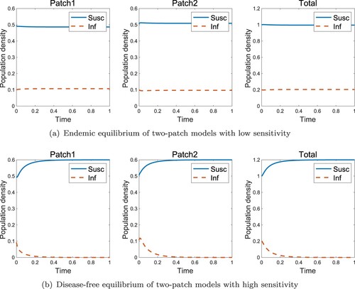
In the high-risk domain, the endemic state always exists regardless of the dispersal rate of the infected individuals when they move uniformly (Figure 4(a)). However, if they move with RID, a disease-free state is obtained, as shown in Figure 4(b). Figure 5 shows the effect of sensitivity when the population is in the high-risk domain. Even if the infected individual moves obeying RID, the disease vanishing is determined by whether the sensitivity $k>k^{\ast }$ or not, where $k^{\ast }$ is defined in Theorem 2.6.

Figure 4. Effect of RID for two-patch models in the high-risk domain (a) Endemic equilibrium without RID (b) Disease-free equilibrium with RID (${\beta }_1=0.05,r_1=0.02,{\beta }_2=0.02,r_2=0.04,d_S=0.1,d_I=0.01$ and k = 6).

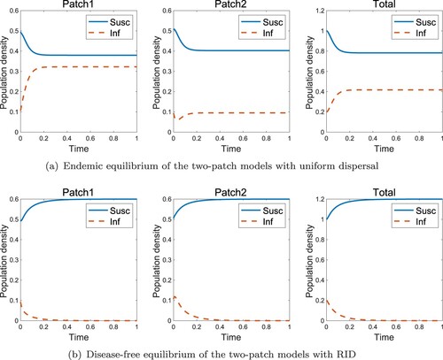
Figure 5. Effect of sensitivity k for two-patch models in the high-risk domain (a) Endemic equilibrium with low sensitivity (k = 3) (b) Disease-free equilibrium with high sensitivity (k = 6) (${\beta }_1=0.05,r_1=0.02,{\beta }_2=0.02,r_2=0.04$, $d_S=0.1$ and $d_I=0.01$).

3. Reaction–diffusion model

In this section, we extend RID to the reaction-diffusion model. As in Section 2, we can define a site-basic reproduction number ${\mathcal{R}}_0^x$ for a location x in a domain Ω by ${\mathcal{R}}_0^x=\beta (x)/r(x),$where $\beta (x)$ and $r(x)$ are boundend functions on $\overline{\mathrm{\Omega }}$, representing the infection rates of the disease and the recovery rate of the disease depending on x, respectively. Then, the infected individuals following the RID strategy determine their dispersal speed depending on ${\mathcal{R}}_0^x$, and such a dispersal rate can be modelled by an increasing function $\delta ({\mathcal{R}}_0^x)$ to ${\mathcal{R}}_0^x$. Here is a simple example: (7) ${\delta }^0({\mathcal{R}}_0^x)=\{\begin{array}{ll}\ell & \text{for}0<{\mathcal{R}}_0^x<1\\ h& \text{for}1<{\mathcal{R}}_0^x<\mathrm{\infty }.\end{array}$(7) Here, ℓ and h are the lower and upper bounds of dispersal rate δ, respectively. This means that if the infected individuals are in a high-risk region ${\mathrm{\Omega }}_{+}:=\{x\in \mathrm{\Omega }:{\mathcal{R}}_0^x>1\},$they escape from the region; furthermore, if the infected individuals are in a low-risk region ${\mathrm{\Omega }}_{-}:=\{x\in \mathrm{\Omega }:{\mathcal{R}}_0^x<1\},$then, they tend to stay in the region. Additionally, we say that Ω is a low-risk domain if ${\int }_{\mathrm{\Omega }}\beta <{\int }_{\mathrm{\Omega }}r$ and a high-risk domain if ${\int }_{\mathrm{\Omega }}\beta >{\int }_{\mathrm{\Omega }}r$.

Then, the patch model with RID can be extended to the reaction-diffusion model as follows: (8) $\{\begin{array}{ll}{S}_t=d_S\mathrm{\Delta }S+I(-\frac{\beta (x)S}{S+I}+r(x))& \\ I_t=\mathrm{\Delta }(\delta (k(x))I)+I(\frac{\beta (x)S}{S+I}-r(x))& \text{in}\mathrm{\Omega }\times (0,\mathrm{\infty }),\\ \mathrm{\nabla S}\cdot \overrightarrow{n}=\mathrm{\nabla }(\delta (k)I)\cdot \overrightarrow{n}=0& \text{on}\mathrm{\partial \Omega }\times (0,\mathrm{\infty }),\\ S(x,0)=S_0(x)\ge 0,I(x,0)=I_0(x)\ge 0& \text{in}\mathrm{\Omega },\end{array}$(8) where $k(x)={\mathcal{R}}_0^x$. $S(x,t)$ and $I(x,t)$ are the densities of susceptible and infected populations in a bounded domain Ω. $d_S,d_I>0$ are the diffusion rates for the susceptible and infected populations, respectively. Let the population size N be defined by $N={\int }_{\mathrm{\Omega }}{S}_0(x)+I_0(x)\mathrm{d}x.$It is noteworthy that the total population size is a constant, i.e. (9) ${\int }_{\mathrm{\Omega }}S(x,t)+I(x,t)\mathrm{d}x=N.$(9) The motility function δ can be treated as a general increasing function, and similar properties can be obtained mathematically. However, threshold values are not explicit to explain. Thus, in this section, we consider an extreme case δ with a form of (7(7) ${\delta }^0({\mathcal{R}}_0^x)=\{\begin{array}{ll}\ell & \text{for}0<{\mathcal{R}}_0^x<1\\ h& \text{for}1<{\mathcal{R}}_0^x<\mathrm{\infty }.\end{array}$(7) ).

Let ${\delta }^0$ be a function defined as (7(7) ${\delta }^0({\mathcal{R}}_0^x)=\{\begin{array}{ll}\ell & \text{for}0<{\mathcal{R}}_0^x<1\\ h& \text{for}1<{\mathcal{R}}_0^x<\mathrm{\infty }.\end{array}$(7) ). The discontinuous function ${\delta }^0$ is approximated by a smooth motility function defined by a convolution, (10) ${\delta }^{\epsilon }(s):={\delta }^0\ast {\eta }^{\epsilon }(s)={\int }_{\mathbb{R}}{\eta }^{\epsilon }(s-y){\delta }^0(y)\mathrm{d}y,$(10) where $\epsilon >0$ is sufficiently small and ${\eta }^{\epsilon }$ is a smooth symmetric mollifier with $\mathrm{supp}{\eta }^{\epsilon }\subset (0,\epsilon )$. Considering the boundedness of β and γ over $\overline{\mathrm{\Omega }}$, and given that s falls within the range $[\underset{\overline{\mathrm{\Omega }}}{min}(\beta /\gamma ),\underset{\overline{\mathrm{\Omega }}}{max}(\beta /\gamma )]$, it is appropriate to define ${\delta }^0(s)=0$ for any s outside this interval in $\mathbb{R}$. As ${\delta }^{\epsilon }$ converges to ${\delta }^0$ in the $L^p(\mathbb{R})$ space for $1\le p<\mathrm{\infty }$, and does so pointwise almost everywhere in s as ε approaches zero, we can view the discontinuous motility function as an approximation in the limit of $\epsilon \to 0$. Instead of the discontinuous function $\delta ={\delta }^0$, we consider δ as $\delta ={\delta }^{\epsilon }$ for sufficiently small ε.

Before introducing the results, we consider the equilibrium solutions of the elliptic system: (11) $\{\begin{array}{ll}{d}_S\mathrm{\Delta }S+I(-\frac{\beta (x)S}{S+I}+r(x))=0& \\ \mathrm{\Delta }(\delta (k)I)+I(\frac{\beta (x)S}{S+I}-r(x))=0& \text{in}\mathrm{\Omega },\\ \mathrm{\nabla S}\cdot \overrightarrow{n}=\mathrm{\nabla }(\delta (k)I)\cdot \overrightarrow{n}=0& \text{on}\mathrm{\partial \Omega },\end{array}$(11) satisfying (12) ${\int }_{\mathrm{\Omega }}(S+I)\mathrm{d}x=N.$(12) Consider the nonnegative solutions $(S,I)$ of (11(11) $\{\begin{array}{ll}{d}_S\mathrm{\Delta }S+I(-\frac{\beta (x)S}{S+I}+r(x))=0& \\ \mathrm{\Delta }(\delta (k)I)+I(\frac{\beta (x)S}{S+I}-r(x))=0& \text{in}\mathrm{\Omega },\\ \mathrm{\nabla S}\cdot \overrightarrow{n}=\mathrm{\nabla }(\delta (k)I)\cdot \overrightarrow{n}=0& \text{on}\mathrm{\partial \Omega },\end{array}$(11) ), S>0. We call a DFE if $I(x)\equiv 0$. An EE is a solution if $I(x)>0$. We denote DFE by $(\hat{S},0)$ and EE by $(S^{\ast },I^{\ast })$.

Now, we define the basic reproduction number ${\mathcal{R}}_0$ for (8(8) $\{\begin{array}{ll}{S}_t=d_S\mathrm{\Delta }S+I(-\frac{\beta (x)S}{S+I}+r(x))& \\ I_t=\mathrm{\Delta }(\delta (k(x))I)+I(\frac{\beta (x)S}{S+I}-r(x))& \text{in}\mathrm{\Omega }\times (0,\mathrm{\infty }),\\ \mathrm{\nabla S}\cdot \overrightarrow{n}=\mathrm{\nabla }(\delta (k)I)\cdot \overrightarrow{n}=0& \text{on}\mathrm{\partial \Omega }\times (0,\mathrm{\infty }),\\ S(x,0)=S_0(x)\ge 0,I(x,0)=I_0(x)\ge 0& \text{in}\mathrm{\Omega },\end{array}$(8) ) : (13) ${\mathcal{R}}_0(k)=\underset{\varphi \in H^1(\mathrm{\Omega }),\varphi \not\equiv 0}{sup}\frac{{\int }_{\mathrm{\Omega }}\frac{\beta }{\delta (k)}{\varphi }^2\mathrm{d}x}{{\int }_{\mathrm{\Omega }}-|\mathrm{\nabla }\varphi {|}^2+\frac{r}{\delta (k)}{\varphi }^2\mathrm{d}x}.$(13) Then, the following results can be obtained. We give the proofs in Appendix.

Theorem 3.1

Let β and r be given.

(i)	If $\beta (x)-r(x)\ge 0$ for all $x\in \mathrm{\Omega }$, then ${\mathcal{R}}_0(k)>1.$
(ii)	If $\beta (x)-r(x)\le 0$ for all $x\in \mathrm{\Omega }$, then ${\mathcal{R}}_0(k)<1$ for any $\ell ,h$.
(iii)	Suppose $\beta (x)-r(x)$ changes sign in Ω. For $\frac{h}{\ell }<M$, ${\mathcal{R}}_0(k)>1$, and for $\frac{h}{\ell }>M$, then there exists the threshold value $d_I^{\ast }(\delta )>0$ such that if $\ell <d_I^{\ast }(\delta )$ then ${\mathcal{R}}_0(k)>1$, and if $\ell >d_I^{\ast }(\delta )$ then ${\mathcal{R}}_0(k)<1$. Moreover, $d_I^{\ast }(\delta )<d_I^{\ast }(d)$.

Theorem 3.2

Let the total population N be fixed. Then,

(i)	if ${\mathcal{R}}_0(k)<1,$ then the DFE is globally asymptotically stable, and
(ii)	if ${\mathcal{R}}_0(k)>1,$ then there is a unique endemic state (EE).

We denote ${\mathcal{R}}_0(d)$ and ${\mathcal{R}}_0(\delta )$ by the basic reproduction numbers of the constant dispersal and RID models, respectively. To compare this, we set $\ell =d$. Then, we have ${\mathcal{R}}_0(\delta )<{\mathcal{R}}_0(d)$. This means that RID is an efficient dispersal strategy to obtain a disease-free state. More precisely, [2, Theorem 2, 3] shows that an EE always exists in the high-risk domain. However, our condition for ${\mathcal{R}}_0(k)<1$ with the sign changing function $\beta -r$ is $\frac{h}{\ell }>M,\ell >{\ell }^{\ast }.$With RID, the sensitivity of the infected individuals $\frac{h}{\ell }$ enables the DFE to be stable for large ℓ. Furthermore, even if their diffusion rate is less than $d_I^{\ast }(d)$, the DFE can be stable for $\ell >d_I^{\ast }(\delta )$ with the RID strategy.

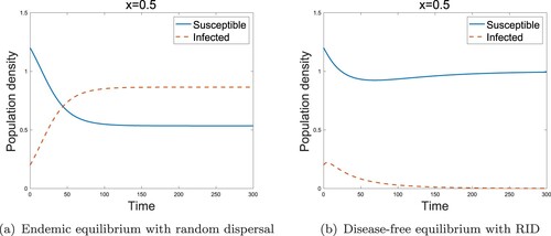
For the reaction-diffusion models, we showed analogous results to the two-patch model. Figure 6 shows that RID could transform the endemic state to a disease-free state in the low-risk domain. In the high-risk domain, we also obtained the result for the role of sensitivity as in the two-patch model. It is evident from Figure 7 that the RID model with high sensitivity, i.e. $h/\ell >M$ leads to the disease-free state. Therefore, we conclude that even though the infected individuals reside in the high-risk domain, the disease can be removed from the region if the infected individuals move with the high sensitivity ($h/\ell$) of RID as they disperse.

Figure 6. Effect of RID for reaction-diffusion models in the low-risk domain (a) Endemic equilibrium without RID (b) Disease-free equilibrium with RID. ($\beta (x)=\sin (2\mathrm{\pi x})+1.2,r(x)=\cos (2\mathrm{\pi x})+1.5$, $d_S=0.01$, $d_I=\ell =0.01$ and h = 0.15.)

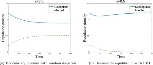
Figure 7. Effect of sensitivity $h/\ell$ for reaction-diffusion models in the high-risk domain (a) Endemic equilibrium without RID (b) Disease-free equilibrium with RID. ($\beta (x)=\sin (2\mathrm{\pi x})+1.5,r(x)=\cos (2\mathrm{\pi x})+1.3$, $d_S=0.01$, $d_I=\ell =0.01$ and h = 0.2.)

4. Conclusion and discussion

This study examines the effectiveness of a resource-based infected dispersal strategy (RID) for controlling infectious diseases in an SIS (susceptible-infected-susceptible) two-patch model and a reaction-diffusion model within spatially heterogeneous environments. The goal was to demonstrate that RID is a more efficient strategy for infected individuals than uniform movement at a constant rate, irrespective of environmental heterogeneity. To substantiate this claim, we examined the existence of unique disease-free equilibria (DFEs) and endemic equilibria (EEs) for the two-patch model and the reaction-diffusion model. We also identified the basic reproduction number, denoted as ${\mathcal{R}}_0$, for both models. The basic reproduction number, ${\mathcal{R}}_0$, is a critical value in infectious disease dynamics. It signifies the average number of new infections generated by a single infectious individual in a completely susceptible population. The value of ${\mathcal{R}}_0$ helps determine whether an infectious disease can spread in a population. If ${\mathcal{R}}_0<1$, the disease will die out over time, implying that the DFE is globally asymptotically stable. In contrast, if ${\mathcal{R}}_0>1$, the disease can spread, resulting in the existence of EE. Our results, proven in Theorems, demonstrate how the RID strategy influences ${\mathcal{R}}_0$. This is achieved through a stability analysis, shedding light on how changes in dispersal strategy can influence the dynamics of infectious diseases. In summary, the results of this study could have important implications for the management and control of infectious diseases. They highlight the potential benefits of strategies that encourage infected individuals to disperse based on resource availability rather than uniform movement, particularly in spatially heterogeneous environments.

In this paper, the scope of our investigation was confined to two-patch models and partial differential equation (PDE) models featuring two variables, which were specifically considered for mathematical analysis. It is an open question whether the results we present can be extended to models with more than two patches or to more general patch models, given the multitude of possible movement rates for infected individuals. One of the main challenges with such extensions is the loss of symmetry in the connectivity matrix as we consider more complex models. However, under certain assumptions about the movement rates, it would be possible to obtain asymptotic profiles for infected individuals, even in these more complex settings. These cases, which have not been explored within the context of two-patch models, will be the focus of a future study. This will allow us to broaden our understanding of how resource-based infected dispersal strategies can be effectively applied in more complex, real-world applications, enhancing our capacity to model and manage infectious disease spread.

Disclosure statement

No potential conflict of interest was reported by the author(s).

Additional information

Funding

This work was supported by the National Research Foundation of Korea (NRF) grant funded by the Korea government (MSIT) (NRF-2022R1F1A1063068),  Ministry of Education (NRF-2021R1A6A3A01086879) and the Korea University Grant.

 

Appendix. Reaction–diffusion model

We consider the reaction–diffusion equations with RID in (8(8) $\{\begin{array}{ll}{S}_t=d_S\mathrm{\Delta }S+I(-\frac{\beta (x)S}{S+I}+r(x))& \\ I_t=\mathrm{\Delta }(\delta (k(x))I)+I(\frac{\beta (x)S}{S+I}-r(x))& \text{in}\mathrm{\Omega }\times (0,\mathrm{\infty }),\\ \mathrm{\nabla S}\cdot \overrightarrow{n}=\mathrm{\nabla }(\delta (k)I)\cdot \overrightarrow{n}=0& \text{on}\mathrm{\partial \Omega }\times (0,\mathrm{\infty }),\\ S(x,0)=S_0(x)\ge 0,I(x,0)=I_0(x)\ge 0& \text{in}\mathrm{\Omega },\end{array}$(8) ). We will show the asymptotic behaviour of the DFE. First, we consider the linearized eigenvalue problem of (8(8) $\{\begin{array}{ll}{S}_t=d_S\mathrm{\Delta }S+I(-\frac{\beta (x)S}{S+I}+r(x))& \\ I_t=\mathrm{\Delta }(\delta (k(x))I)+I(\frac{\beta (x)S}{S+I}-r(x))& \text{in}\mathrm{\Omega }\times (0,\mathrm{\infty }),\\ \mathrm{\nabla S}\cdot \overrightarrow{n}=\mathrm{\nabla }(\delta (k)I)\cdot \overrightarrow{n}=0& \text{on}\mathrm{\partial \Omega }\times (0,\mathrm{\infty }),\\ S(x,0)=S_0(x)\ge 0,I(x,0)=I_0(x)\ge 0& \text{in}\mathrm{\Omega },\end{array}$(8) ). Let $\tilde{I}=\delta (k)I$. Then (8(8) $\{\begin{array}{ll}{S}_t=d_S\mathrm{\Delta }S+I(-\frac{\beta (x)S}{S+I}+r(x))& \\ I_t=\mathrm{\Delta }(\delta (k(x))I)+I(\frac{\beta (x)S}{S+I}-r(x))& \text{in}\mathrm{\Omega }\times (0,\mathrm{\infty }),\\ \mathrm{\nabla S}\cdot \overrightarrow{n}=\mathrm{\nabla }(\delta (k)I)\cdot \overrightarrow{n}=0& \text{on}\mathrm{\partial \Omega }\times (0,\mathrm{\infty }),\\ S(x,0)=S_0(x)\ge 0,I(x,0)=I_0(x)\ge 0& \text{in}\mathrm{\Omega },\end{array}$(8) ) can be written as: (A1) $\{\begin{array}{ll}{S}_t=d_S\mathrm{\Delta }S+I(-\frac{\beta (x)S}{S+I}+r(x))& \\ {\tilde{I}}_t=\delta (k)[\mathrm{\Delta }\tilde{I}+I(\frac{\beta (x)S}{S+I}-r(x))]& \text{in}\mathrm{\Omega }\times (0,\mathrm{\infty }),\\ \mathrm{\nabla S}\cdot \overrightarrow{n}=\mathrm{\nabla }\tilde{I}\cdot \overrightarrow{n}=0& \text{on}\mathrm{\partial \Omega }\times (0,\mathrm{\infty }),\\ S(x,0)=S_0(x)\ge 0,\tilde{I}(x,0)={\tilde{I}}_0(x)\ge 0& \text{in}\mathrm{\Omega },\end{array}$(A1) where $\widetilde{I_0}=\delta (k)I_0.$ For a fixed total population size N, it is easy to check that $(N/|\mathrm{\Omega }|,0)$ is a unique semitrivial solution of (A1(A1) $\{\begin{array}{ll}{S}_t=d_S\mathrm{\Delta }S+I(-\frac{\beta (x)S}{S+I}+r(x))& \\ {\tilde{I}}_t=\delta (k)[\mathrm{\Delta }\tilde{I}+I(\frac{\beta (x)S}{S+I}-r(x))]& \text{in}\mathrm{\Omega }\times (0,\mathrm{\infty }),\\ \mathrm{\nabla S}\cdot \overrightarrow{n}=\mathrm{\nabla }\tilde{I}\cdot \overrightarrow{n}=0& \text{on}\mathrm{\partial \Omega }\times (0,\mathrm{\infty }),\\ S(x,0)=S_0(x)\ge 0,\tilde{I}(x,0)={\tilde{I}}_0(x)\ge 0& \text{in}\mathrm{\Omega },\end{array}$(A1) ).

Lemma A.1

Let the total population N be fixed. Then, (8(8) $\{\begin{array}{ll}{S}_t=d_S\mathrm{\Delta }S+I(-\frac{\beta (x)S}{S+I}+r(x))& \\ I_t=\mathrm{\Delta }(\delta (k(x))I)+I(\frac{\beta (x)S}{S+I}-r(x))& \text{in}\mathrm{\Omega }\times (0,\mathrm{\infty }),\\ \mathrm{\nabla S}\cdot \overrightarrow{n}=\mathrm{\nabla }(\delta (k)I)\cdot \overrightarrow{n}=0& \text{on}\mathrm{\partial \Omega }\times (0,\mathrm{\infty }),\\ S(x,0)=S_0(x)\ge 0,I(x,0)=I_0(x)\ge 0& \text{in}\mathrm{\Omega },\end{array}$(8) ) has a unique DFE where $(\hat{S},0)=(N/|\mathrm{\Omega }|,0)$.

A.1. Linear stability of DFE

Let $g(x,S,\tilde{I})=I(-\frac{\beta (x)S}{S+I}+r(x))$ and $h(x,S,\tilde{I})=I(\frac{\beta (x)S}{S+I}-r(x))$. Then, by simple calculations, we obtain $\left(\begin{array}{cc}{g}_S& g_{\tilde{I}}\\ h_S& g_{\tilde{I}}\end{array}\right)=\left(\begin{array}{cc}-\frac{\beta (x)I^2}{(S+I{)}^2}& \frac{1}{\delta (k)}(-\frac{\beta (x)S}{S+I}+r(x)-\frac{\beta (x)\mathrm{SI}}{(S+I{)}^2})\\ \frac{\beta (x)I^2}{(S+I{)}^2}& \frac{1}{\delta (k)}(\frac{\beta (x)S}{S+I}-r(x)+\frac{\beta (x)\mathrm{SI}}{(S+I{)}^2})\end{array}\right).$Then, we obtain the linearized eigenvalue problem at $(\hat{S},0)$: (A2) $\{\begin{array}{ll}\mathrm{\lambda \varphi }=d_S\mathrm{\Delta \varphi }+\frac{1}{\delta (k)}(-\beta (x)+r(x))\psi & \\ \mathrm{\lambda \psi }=\delta (k)[\mathrm{\Delta \psi }+\frac{1}{\delta (k)}(\beta (x)-r(x))\psi ]& \text{in}\mathrm{\Omega },\\ \mathrm{\nabla \varphi }\cdot \overrightarrow{n}=\mathrm{\nabla \psi }\cdot \overrightarrow{n}=0& \text{on}\mathrm{\partial \Omega }.\end{array}$(A2) For the linear stability of $(\hat{S},0)$, we introduce a lemma:

Lemma A.2

If ${\lambda }_1(\mathrm{\Delta }+\frac{1}{\delta (k)}(\beta (x)-r(x)))>0$, then, $(\hat{S},0)$ is locally asymptotically unstable, and if ${\lambda }_1(\mathrm{\Delta }+\frac{1}{\delta (k)}(\beta (x)-r(x)))<0$, then $(\hat{S},0)$ is locally asymptotically stable.

Proof.

First, suppose ${\lambda }_1(\mathrm{\Delta }+\frac{\beta (x)-r(x)}{\delta (k)})>0$ and we denote ${\lambda }_1(\mathrm{\Delta }+\frac{\beta (x)-r(x)}{\delta (k)})$ by ${\lambda }_1$. We consider an eigenvalue problem $\{\begin{array}{ll}\mathrm{k\psi }=\mathrm{\Delta \psi }+\frac{1}{\delta (k)}(\beta (x)-r(x))\psi -\frac{\lambda }{\delta (k)}\psi & \text{in}\mathrm{\Omega },\\ 0=\mathrm{\nabla \psi }\cdot \overrightarrow{n}& \text{on}\mathrm{\partial \Omega }.\end{array}$and denote the principal eigenvalue by $k^{\lambda }$. When $\lambda =0$, $k^{\lambda }={\lambda }_1>0$. Moreover, $k^{\lambda }$ will be negative for sufficiently large λ. Thus, there exists $\lambda >0$ such that $k^{\lambda }=0$. It can be easily shown that $L=d_S\mathrm{\Delta }-\lambda$is invertible. Thus, $\lambda >0$ is an eigenvalue of (A2(A2) $\{\begin{array}{ll}\mathrm{\lambda \varphi }=d_S\mathrm{\Delta \varphi }+\frac{1}{\delta (k)}(-\beta (x)+r(x))\psi & \\ \mathrm{\lambda \psi }=\delta (k)[\mathrm{\Delta \psi }+\frac{1}{\delta (k)}(\beta (x)-r(x))\psi ]& \text{in}\mathrm{\Omega },\\ \mathrm{\nabla \varphi }\cdot \overrightarrow{n}=\mathrm{\nabla \psi }\cdot \overrightarrow{n}=0& \text{on}\mathrm{\partial \Omega }.\end{array}$(A2) ), which implies that $(\hat{S},0)$ is locally unstable.

Next, we assume that ${\lambda }_1(\mathrm{\Delta }+\frac{\beta (x)-r(x)}{\delta (k)})<0$. Suppose that (A2(A2) $\{\begin{array}{ll}\mathrm{\lambda \varphi }=d_S\mathrm{\Delta \varphi }+\frac{1}{\delta (k)}(-\beta (x)+r(x))\psi & \\ \mathrm{\lambda \psi }=\delta (k)[\mathrm{\Delta \psi }+\frac{1}{\delta (k)}(\beta (x)-r(x))\psi ]& \text{in}\mathrm{\Omega },\\ \mathrm{\nabla \varphi }\cdot \overrightarrow{n}=\mathrm{\nabla \psi }\cdot \overrightarrow{n}=0& \text{on}\mathrm{\partial \Omega }.\end{array}$(A2) ) has a nonnegative eigenvalue $\lambda \ge 0$ with the corresponding eigenvalue $({\varphi }_1,{\psi }_1)$. Suppose that ${\psi }_1\equiv 0$. By multiplying ${\varphi }_1$ and integrating, we obtain ${\int }_{\mathrm{\Omega }}\lambda {\varphi }_1^2={\int }_{\mathrm{\Omega }}{d}_S{\varphi }_1\mathrm{\Delta }{\varphi }_1={\int }_{\mathrm{\Omega }}-d_S|\mathrm{\nabla }{\varphi }_1{|}^2<0.$This is a contradiction. Hence, ${\psi }_1\not\equiv 0$. However, this yields that $\begin{array}{rl}{\lambda }_1& =\underset{\psi \in H^1\setminus \{0\}}{sup}\frac{{\int }_{\mathrm{\Omega }}-|\mathrm{\nabla }\psi {|}^2+\frac{\beta (x)-r(x)}{\delta (k)}{\psi }^2}{{\int }_{\mathrm{\Omega }}{\psi }^2}\\ & \ge \frac{{\int }_{\mathrm{\Omega }}-|\mathrm{\nabla }{\psi }_1{|}^2+\frac{\beta (x)-r(x)}{\delta (k)}{\psi }_1^2}{{\int }_{\mathrm{\Omega }}{\psi }_1^2}=\frac{{\int }_{\mathrm{\Omega }}\frac{\lambda }{\delta (k)}{\psi }_1^2}{{\int }_{\mathrm{\Omega }}{\psi }_1^2}\ge 0.\end{array}$This is also a contradiction. Thus, $(\hat{S},0)$ is locally unstable.

For simplicity, we denote ${\lambda }_1(\mathrm{\Delta }+\frac{1}{\delta (k)}(\beta (x)-r(x)))$ by ${\lambda }_1$ and define $M:=\frac{{\int }_{{\mathrm{\Omega }}_{+}}\beta -r}{{\int }_{{\mathrm{\Omega }}_{-}}r-\beta }.$The value M indicates the degree of infection in the domain. For example, if M>1, then the given domain is occupied more by the high-risk region.

Divide the set ${\mathrm{\Omega }}_{+}={\mathrm{\Omega }}_{+,1}\cup {\mathrm{\Omega }}_{+,\epsilon }$, where ${\mathrm{\Omega }}_{+,1}=\{x\in \mathrm{\Omega }:\beta (x)/r(x)\ge 1+\epsilon \}$ and ${\mathrm{\Omega }}_{+,\epsilon }=\{x\in \mathrm{\Omega }:1<\beta (x)/r(x)<1+\epsilon \}.$ Recall that $\delta ={\delta }^{\epsilon }$ defined by (10(10) ${\delta }^{\epsilon }(s):={\delta }^0\ast {\eta }^{\epsilon }(s)={\int }_{\mathbb{R}}{\eta }^{\epsilon }(s-y){\delta }^0(y)\mathrm{d}y,$(10) ). Before we discuss the eigenvalue problem, we first show the following lemma:

Lemma A.3

For given $\delta ,\ell$, and h,

(i)	If $\beta (x)-r(x)\ge 0$ for all $x\in \mathrm{\Omega }$, then ${\int }_{\mathrm{\Omega }}\frac{1}{\delta (k)}(\beta (x)-r(x))>0$.
(ii)	If $\beta (x)-r(x)\le 0$ for all $x\in \mathrm{\Omega }$, then ${\int }_{\mathrm{\Omega }}\frac{1}{\delta (k)}(\beta (x)-r(x))<0$.
(iii)	Suppose that $\beta (x)-r(x)$ changes sign in Ω. If $\frac{h}{\ell }<M$, then ${\int }_{\mathrm{\Omega }}\frac{1}{\delta (k)}(\beta (x)-r(x))>0$, and if $\frac{h}{\ell }>M$, then ${\int }_{\mathrm{\Omega }}\frac{1}{\delta (k)}(\beta (x)-r(x))<0$ for sufficiently small $\epsilon >0$.

Proof.

(i) and (ii) are obvious.

(iii) We assume that $\beta (x)-r(x)$ changes sign in Ω. Since ${\mathrm{\Omega }}_{+}$ and ${\mathrm{\Omega }}_{-}$ are nonempty, we have ${\int }_{{\mathrm{\Omega }}_{+}}\frac{\beta -r}{h}+{\int }_{{\mathrm{\Omega }}_{-}}\frac{\beta -r}{\ell }>0⟺\frac{h}{\ell }<\frac{{\int }_{{\mathrm{\Omega }}_{+}}\beta -r}{{\int }_{{\mathrm{\Omega }}_{-}}r-\beta }.$Since ${\mathrm{\Omega }}_{+,1}\to {\mathrm{\Omega }}_{+}$ and the integration over ${\mathrm{\Omega }}_{+,\epsilon }$ converges to 0 as $\epsilon \to 0$, we have ${\int }_{\mathrm{\Omega }}\frac{\beta -r}{\delta (k)}={\int }_{{\mathrm{\Omega }}_{+,1}}\frac{\beta -r}{h}+{\int }_{{\mathrm{\Omega }}_{+,\epsilon }}\frac{\beta -r}{\delta (k)}+{\int }_{{\mathrm{\Omega }}_{-}}\frac{\beta -r}{\ell }>0$for sufficiently small $\epsilon >0$ if $\frac{h}{\ell }<M$. Similarly, ${\int }_{\mathrm{\Omega }}\frac{\beta -r}{\delta (k)}<0$ if $\frac{h}{\ell }>M$ for sufficiently small $\epsilon >0.$

Therefore, we obtain the following result for the linear stability of $(\hat{S},0)$:

Theorem A.4

Let β and r be given.

(i)	If $\beta (x)-r(x)\ge 0$ for all $x\in \mathrm{\Omega }$, then $(\hat{S},0)$ is locally asymptotically unstable for any $\ell ,h$.
(ii)	If $\beta (x)-r(x)\le 0$ for all $x\in \mathrm{\Omega }$, then $(\hat{S},0)$ is locally asymptotically stable for any $\ell ,h$.
(iii)	Suppose $\beta (x)-r(x)$ changes sign in Ω. For $\frac{h}{\ell }<M$, $(\hat{S},0)$ is locally asymptotically unstable, and for $\frac{h}{\ell }>M$, then there exists the threshold value $d_I^{\ast }(\delta )>d_I^{\ast }(d)$ such that if $\ell <d_I^{\ast }(\delta )$ then $(\hat{S},0)$ is locally asymptotically unstable, and if $\ell >d_I^{\ast }(\delta )$ then $(\hat{S},0)$ is locally asymptotically stable for a sufficiently small $\epsilon >0$.

Proof.

By Lemma A.2, we only need to check the sign of ${\lambda }_1$.

1. Suppose that $\beta (x)-r(x)\ge 0$ for all $x\in \mathrm{\Omega }$. Then, $\begin{array}{rl}{\lambda }_1& =\underset{\varphi \in H^1(\mathrm{\Omega }),\varphi \not\equiv 0}{sup}\frac{{\int }_{\mathrm{\Omega }}-|\mathrm{\nabla }\varphi {|}^2+\frac{1}{\delta (k)}(\beta (x)-r(x)){\varphi }^2}{{\int }_{\mathrm{\Omega }}{\varphi }^2}\\ & \ge \frac{1}{|\mathrm{\Omega }|}{\int }_{\mathrm{\Omega }}\frac{1}{\delta (k)}(\beta (x)-r(x))>0.\end{array}$

2. Next, we assume that $\beta (x)-r(x)\le 0$ for all $x\in \mathrm{\Omega }$. Let ${\varphi }_1$ be the principal eigenfunction with respect to ${\lambda }_1$ such that $||{\varphi }_1|{|}_2=1$. Then, we obtain ${\lambda }_1={\int }_{\mathrm{\Omega }}-|\mathrm{\nabla }{\varphi }_1{|}^2+\frac{1}{\delta (k)}(\beta (x)-r(x)){\varphi }_1^2<0.$

3. Suppose that $\beta (x)-r(x)$ changes sign in Ω. For the case $\frac{h}{\ell }<M$, then for sufficiently small $\epsilon >0$, we have ${\int }_{\mathrm{\Omega }}\frac{\beta -r}{\delta (k)}>0.$By a similar process to (i), we have ${\lambda }_1>0$.

Next, we assume $\frac{h}{\ell }>M$. Then, ${\int }_{\mathrm{\Omega }}\frac{\beta -r}{\delta (k)}<0$ for sufficiently small $\epsilon >0$. We set $\ell =d_I^{\ast }(d)$ where $d_I^{\ast }(d)$ is from [2, Theorem 2] that satisfies ${\lambda }_1(d_I^{\ast }(d)\mathrm{\Delta }+(\beta (x)-r(x)))=0.$ By the definition of the principal eigenvalue, ${\lambda }_1(d_I^{\ast }(d)\mathrm{\Delta }+(\beta (x)-r(x)))({\varphi }_1)\le 0$. Thus, $\begin{array}{rl}{\lambda }_1& ={\int }_{\mathrm{\Omega }}-|\mathrm{\nabla }{\varphi }_1{|}^2+\frac{1}{\delta (k)}(\beta (x)-r(x)){\varphi }_1^2\\ & ={\int }_{{\mathrm{\Omega }}_{+}}-|\mathrm{\nabla }{\varphi }_1{|}^2+\frac{1}{\delta (k)}(\beta (x)-r(x)){\varphi }_1^2+{\int }_{{\mathrm{\Omega }}_{-}}-|\mathrm{\nabla }{\varphi }_1{|}^2+\frac{1}{\ell }(\beta (x)-r(x)){\varphi }_1^2\\ & <{\int }_{{\mathrm{\Omega }}_{+}}-|\mathrm{\nabla }{\varphi }_1{|}^2+\frac{1}{\ell }(\beta (x)-r(x)){\varphi }_1^2+{\int }_{{\mathrm{\Omega }}_{-}}-|\mathrm{\nabla }{\varphi }_1{|}^2+\frac{1}{\ell }(\beta (x)-r(x)){\varphi }_1^2\\ & ={\int }_{\mathrm{\Omega }}-|\mathrm{\nabla }{\varphi }_1{|}^2+\frac{1}{d_I^{\ast }(d)}(\beta (x)-r(x)){\varphi }_1^2\le 0.\end{array}$The inequality holds from the fact that $\delta (k)\ge \ell$ in ${\mathrm{\Omega }}_{+}$. Let ψ be a test function supported in ${\mathrm{\Omega }}_{+,1}$. Let $p=\frac{h}{\ell }>M$ be a fixed value. Then we can represent $h=\mathrm{p\ell }$. Thus $\begin{array}{rl}{\lambda }_1& =\underset{\varphi \in H^1(\mathrm{\Omega }),\varphi \not\equiv 0}{sup}{\int }_{\mathrm{\Omega }}-|\mathrm{\nabla \varphi }{|}^2+\frac{1}{\delta (k)}(\beta (x)-r(x)){\varphi }^2\\ & \ge {\int }_{\mathrm{\Omega }}-|\mathrm{\nabla \psi }{|}^2+\frac{1}{\delta (k)}(\beta (x)-r(x)){\psi }^2\\ & ={\int }_{{\mathrm{\Omega }}_{+,1}}-|\mathrm{\nabla \psi }{|}^2+\frac{1}{\mathrm{p\ell }}(\beta (x)-r(x)){\psi }^2>0,\end{array}$for sufficiently small ℓ. Since $\ell {\lambda }_1$ is a decreasing function for ℓ, there exists $d_I^{\ast }(\delta )<d_I^{\ast }(d)$ such that ${\lambda }_1=0$ for $\ell ={\ell }^{\ast }$.

A.2. Basic reproduction number and EE

We define the basic reproduction number ${\mathcal{R}}_0$ for (8(8) $\{\begin{array}{ll}{S}_t=d_S\mathrm{\Delta }S+I(-\frac{\beta (x)S}{S+I}+r(x))& \\ I_t=\mathrm{\Delta }(\delta (k(x))I)+I(\frac{\beta (x)S}{S+I}-r(x))& \text{in}\mathrm{\Omega }\times (0,\mathrm{\infty }),\\ \mathrm{\nabla S}\cdot \overrightarrow{n}=\mathrm{\nabla }(\delta (k)I)\cdot \overrightarrow{n}=0& \text{on}\mathrm{\partial \Omega }\times (0,\mathrm{\infty }),\\ S(x,0)=S_0(x)\ge 0,I(x,0)=I_0(x)\ge 0& \text{in}\mathrm{\Omega },\end{array}$(8) ) : (A3) ${\mathcal{R}}_0(k)=\underset{\varphi \in H^1(\mathrm{\Omega }),\varphi \not\equiv 0}{sup}\frac{{\int }_{\mathrm{\Omega }}\frac{\beta }{\delta (k)}{\varphi }^2\mathrm{d}x}{{\int }_{\mathrm{\Omega }}-|\mathrm{\nabla }\varphi {|}^2+\frac{r}{\delta (k)}{\varphi }^2\mathrm{d}x}.$(A3) Then, we have the following lemma whose proof is analogous to the proof of Lemma 2.3 in [2]. Thus, we omit the proof.

Lemma A.5

${\mathcal{R}}_0(k)>1$ when ${\lambda }_1>0$, and ${\mathcal{R}}_0(k)<1$ when ${\lambda }_1<0$.

Now, we show that EE exists when ${\mathcal{R}}_0(k)>1$. This is similar to the proof in [2]. First, we consider the alternative of (11(11) $\{\begin{array}{ll}{d}_S\mathrm{\Delta }S+I(-\frac{\beta (x)S}{S+I}+r(x))=0& \\ \mathrm{\Delta }(\delta (k)I)+I(\frac{\beta (x)S}{S+I}-r(x))=0& \text{in}\mathrm{\Omega },\\ \mathrm{\nabla S}\cdot \overrightarrow{n}=\mathrm{\nabla }(\delta (k)I)\cdot \overrightarrow{n}=0& \text{on}\mathrm{\partial \Omega },\end{array}$(11) ) as follows: (A4) $\{\begin{array}{ll}\tau =d_{S}S+\delta (k)I& \\ 0=\mathrm{\Delta }(\delta (k)I)+I(\beta -r-\frac{\mathrm{\beta I}}{S+I})& \text{in}\mathrm{\Omega },\\ 0=\mathrm{\nabla S}\cdot \overrightarrow{n}=\mathrm{\nabla }(\delta (k)I)\cdot \overrightarrow{n}& \text{on}\mathrm{\partial \Omega },\\ N={\int }_{\mathrm{\Omega }}(S+I)\mathrm{d}x,& \end{array}$(A4) where τ is some positive constant. Let $\tilde{S}=\frac{S}{\tau }$, $\tilde{I}=\frac{\delta (k)I}{\tau },$ and $f(x,u)=\frac{1}{\delta (k)}[\beta (x)(1-\frac{d_{S}u}{d_{S}u+\delta (k)(1-u)})-r(x)].$Note that f is strictly decreasing as $\frac{1}{\delta (k)}(\beta (x)-r(x))$ to $-r(x)/\delta (k)$ as u increases from 0 to 1. Hence, we have the equivalent representation: (A5) $\{\begin{array}{ll}1=d_S\tilde{S}+\tilde{I}& \\ 0=\mathrm{\Delta }\tilde{I}+\tilde{I}f(x,\tilde{I})& \text{in}\mathrm{\Omega },\\ 0=\mathrm{\nabla }\tilde{I}\cdot \overrightarrow{n}& \text{on}\mathrm{\partial \Omega },\\ \tau =\frac{N}{{\int }_{\mathrm{\Omega }}\tilde{S}+\tilde{I}/\delta (k)}.& \end{array}$(A5) Therefore, we introduce a lemma.

Lemma A.6

Suppose that ${\mathcal{R}}_0(k)>1$. Then, (A5(A5) $\{\begin{array}{ll}1=d_S\tilde{S}+\tilde{I}& \\ 0=\mathrm{\Delta }\tilde{I}+\tilde{I}f(x,\tilde{I})& \text{in}\mathrm{\Omega },\\ 0=\mathrm{\nabla }\tilde{I}\cdot \overrightarrow{n}& \text{on}\mathrm{\partial \Omega },\\ \tau =\frac{N}{{\int }_{\mathrm{\Omega }}\tilde{S}+\tilde{I}/\delta (k)}.& \end{array}$(A5) ) has a nonnegative solution $(\tilde{S},\tilde{I})$ satisfying $\tilde{S},\tilde{I}\in C^2(\overline{\mathrm{\Omega }})$ and $I\not\equiv 0$ on Ω. Furthermore, $\tilde{I}$ is unique, $\tilde{S}>0$ and $0<\tilde{I}<1$.

Proof.

By using the upper-lower solution method and the maximum principle, we can obtain the desired result. (See details in [2])

Hence, the following lemma holds.

Lemma A.7

Suppose that ${\mathcal{R}}_0(k)>1$. Then, (11(11) $\{\begin{array}{ll}{d}_S\mathrm{\Delta }S+I(-\frac{\beta (x)S}{S+I}+r(x))=0& \\ \mathrm{\Delta }(\delta (k)I)+I(\frac{\beta (x)S}{S+I}-r(x))=0& \text{in}\mathrm{\Omega },\\ \mathrm{\nabla S}\cdot \overrightarrow{n}=\mathrm{\nabla }(\delta (k)I)\cdot \overrightarrow{n}=0& \text{on}\mathrm{\partial \Omega },\end{array}$(11) ) has a unique EE, $(S^{\ast },I^{\ast })$, given by $(S^{\ast },I^{\ast })=(\tau \tilde{S},\tau \tilde{I}/\delta (k))$ such that $S^{\ast },I^{\ast }\in C^2(\overline{\mathrm{\Omega }})$ and $I^{\ast }\not\equiv 0$ on Ω, where $\tau ,\tilde{S},$ and $\tilde{I}$ are as in (A5(A5) $\{\begin{array}{ll}1=d_S\tilde{S}+\tilde{I}& \\ 0=\mathrm{\Delta }\tilde{I}+\tilde{I}f(x,\tilde{I})& \text{in}\mathrm{\Omega },\\ 0=\mathrm{\nabla }\tilde{I}\cdot \overrightarrow{n}& \text{on}\mathrm{\partial \Omega },\\ \tau =\frac{N}{{\int }_{\mathrm{\Omega }}\tilde{S}+\tilde{I}/\delta (k)}.& \end{array}$(A5) ).

Combining the results above, we obtain the following:

Theorem A.8

Let the total population N be fixed. Then

(i)	if ${\mathcal{R}}_0(k)<1,$ then the DFE is globally asymptotically stable, and
(ii)	if ${\mathcal{R}}_0(k)>1,$ then there is a unique endemic state (EE).

Proof.

It can be proved in a similar way to the proof in [2]. For the reader's convenience, we present a sketch of the proof.

(i) Let $(\overline{S},\overline{I})$ be a solution of (8(8) $\{\begin{array}{ll}{S}_t=d_S\mathrm{\Delta }S+I(-\frac{\beta (x)S}{S+I}+r(x))& \\ I_t=\mathrm{\Delta }(\delta (k(x))I)+I(\frac{\beta (x)S}{S+I}-r(x))& \text{in}\mathrm{\Omega }\times (0,\mathrm{\infty }),\\ \mathrm{\nabla S}\cdot \overrightarrow{n}=\mathrm{\nabla }(\delta (k)I)\cdot \overrightarrow{n}=0& \text{on}\mathrm{\partial \Omega }\times (0,\mathrm{\infty }),\\ S(x,0)=S_0(x)\ge 0,I(x,0)=I_0(x)\ge 0& \text{in}\mathrm{\Omega },\end{array}$(8) ). By Theorem A.4 and Lemma A.2, the DFE is locally asymptotically stable. By the similar argument in Lemma A.2, ${\lambda }_1(\delta (k)[\mathrm{\Delta }+\frac{\beta (x)-r(x)}{\delta (k)}])<0$, denoted by ${\lambda }^{\ast }$. Let ${\psi }^{\ast }>0$ be the principal eigenvalue with respect to ${\lambda }^{\ast }$. If we define $u(x,t)=M{e}^{{\lambda }^{\ast }t}{\psi }^{\ast }$ where M is large constant such that $\tilde{I}(x,0)\le u(x,0)$ and use the comparison principle, we can obtain $\overline{I}(x,t)\to 0$ as $t\to \mathrm{\infty }$.

It remains to show that $\underset{t\to \mathrm{\infty }}{lim}\overline{S}=\hat{S}$. From the boundedness and continuity of $\delta ,\beta ,$ and r, $|\frac{\mathrm{\partial }\overline{S}}{\mathrm{\partial }t}-d_S\mathrm{\Delta }\overline{S}|\le C_1{e}^{{\lambda }^{\ast }t}\to 0\text{as}t\to \mathrm{\infty },$for some constant $C_1>0$. Therefore, $\overline{S}(x,t)$ converges to some positive constant $C^{\ast }$ as $t\to \mathrm{\infty }$.

If we show $C^{\ast }=\hat{S}$, our proof is done. To show this, we write $\overline{S}(x,t)=S_1(t)+S_2(x,t)$ where $S_1(t)=\frac{1}{|\mathrm{\Omega }|}{\int }_{\mathrm{\Omega }}\overline{S}(x,t)$. Using the boundedness of $\delta ,\beta ,$ and r, we can get $\left|\frac{\mathrm{\partial }}{\mathrm{\partial }t}{\int }_{\mathrm{\Omega }}\overline{S}(x,t)\mathrm{d}x\right|\le C{e}^{{\lambda }^{\ast }t},\left|\frac{\mathrm{\partial }{S}_1}{\mathrm{\partial }t}\right|\le C_2{e}^{{\lambda }^{\ast }t}$for a generic constant C>0. From this, $S_2$ satisfies $\mathrm{\partial }{S}_2/\mathrm{\partial }t=d_S\mathrm{\Delta }{S}_2+f(x,t)\text{with}|f(x,t)|\le C_2{e}^{{\lambda }^{\ast }t}$for some constant $C_3>0$. Since ${\int }_{\mathrm{\Omega }}{S}_2(x,t)\mathrm{d}x=0$ for all $t\ge 0$ and $\overline{I}(x,t)\to 0$ as $t\to \mathrm{\infty }$ and (9(9) ${\int }_{\mathrm{\Omega }}S(x,t)+I(x,t)\mathrm{d}x=N.$(9) ), $S_1(t)\to \hat{S}$ as $t\to \mathrm{\infty }$.

Finally, we show that $\underset{t\to \mathrm{\infty }}{lim}{S}_2(x,t)=0$. Let $\{{\phi }_k\}$ be the normalized eigenfunctions with $\{{\mu }_k\},$ which are eigenvalues of Δ with the Neumann boundary condition. If we set $S_2=\sum _{k=0}^{\mathrm{\infty }}{a}_k(t){\phi }_k(x)$ and $f(x,t)=\sum _{k=0}^{\mathrm{\infty }}{b}_k(t){\phi }_k(x)$, we have $|b_k(t)|\le C_3{e}^{{\lambda }^{\ast }t},|a_k(t)|\le C_4{e}^{{\lambda }^{\ast \ast }t}\text{for every}k\ge 1,$where $C_3$ and $C_4$ are positive constants and ${\lambda }^{\ast \ast }=max\{{\mu }_1,{\lambda }^{\ast }\}<0$. Hence, $S_2(x,t)$ goes to 0 as $t\to 0$. Therefore, $\underset{t\to \mathrm{\infty }}{lim}\hat{S}(x,t)=\hat{S}$ for all $x\in \mathrm{\Omega }$.

(ii) By Theorem A.4 and Lemma A.2, an EE exists when ${\mathcal{R}}_0(k)>1$.

References

- LJS Allen, BM Bolker, Y Lou, et al. Asymptotic profiles of the steady states for an SIS epidemic patch model. SIAM J Appl Math. 2007;67(5):1283–1309. doi: 10.1137/060672522
- LJS Allen, BM Bolker, Y Lou, et al. Asymptotic profiles of the steady states for an SIS epidemic reaction-diffusion model. Discrete Contin Dyn Syst. 2008;21(1):1–20. doi: 10.3934/dcds.2008.21.1
- LJ Allen, Y Lou, AL Nevai. Spatial patterns in a discrete-time SIS patch model. J Math Biol. 2009;58(3):339–375. doi: 10.1007/s00285-008-0194-y
- BM Bolker, BT Grenfell. Space, persistence, and dynamics of measles epidemics. Philos Trans R Soc Lond B. 1995;348:309–320. doi: 10.1098/rstb.1995.0070
- C Castillo-Chavez, A-A Yakubu. Dispersal, disease and life-history evolution. Math Biosci. 2001;173:35–53. doi: 10.1016/S0025-5564(01)00065-7
- C Castillo-Chavez, A-A Yakubu. Intraspecific competition, dispersal, and disease dynamics in discrete-time patchy environments. In: Castillo-Chavez C, Blower S, van den Driessche P, Kirschner D, and Yakubu A-A, editors. Mathematical approaches for emerging and reemerging infectious diseases: an introduction. New York: Springer-Verlag; 2002. p. 165–181.
- G Hess. Disease in metapopulation models: implications for conservation. Ecology. 1996;77:1617–1632. doi: 10.2307/2265556
- A Lloyd, RM May. Spatial heterogeneity in epidemic models. J Theor Biol. 1996;179:1–11. doi: 10.1006/jtbi.1996.0042
- S Ruan. Spatial-temporal dynamics in nonlocal epidemiological models. In: Takeuchi Y, Sato K, and Iwasa Y, editors. Mathematics for life science and medicine, Vol. 2. New York: Springer-Verlag; 2006. p. 99–122.
- M Salmani, P van den Driessche. A model for disease transmission in a patchy environment. Discrete Contin Dyn Syst Ser B. 2006;6:185–202.
- J Arino, JR Jordan, P van den Driessche. Quarantine in a multi-species epidemic model with spatial dynamics. Math Biosci. 2007;206:46–60. doi: 10.1016/j.mbs.2005.09.002
- T Dhirasakdanon, HR Thieme, P Van Den Driessche. A sharp threshold for disease persistence in host metapopulations. J Biol Dyn. 2007;1(4):363–378. doi: 10.1080/17513750701605465
- Y-H Hsieh, P van den Driessche, L Wang. Impact of travel between patches for spatial spread of disease. Bull Math Biol. 2007;69:1355–1375. doi: 10.1007/s11538-006-9169-6
- MA Lewis, J Renclawowicz, P van den Driessche. Traveling waves and spread rates for a West Nile virus model. Bull Math Biol. 2006;68(1):3–23. doi: 10.1007/s11538-005-9018-z
- EB Postnikov, IM Sokolov. Continuum description of a contact infection spread in a SIR model. Math Biosci. 2007;208:205–215. doi: 10.1016/j.mbs.2006.10.004
- S Chen, J Shi, Z Shuai, et al. Asymptotic profiles of the steady states for an SIS epidemic patch model with asymmetric connectivity matrix. J Math Biol. 2020;80(7):2327–2361. doi: 10.1007/s00285-020-01497-8
- K Kuto, H Matsuzawa, R Peng. Concentration profile of endemic equilibrium of a reaction–diffusion–advection SIS epidemic model. Calc Var Partial Differ Equ. 2017;56(4):112. doi: 10.1007/s00526-017-1207-8
- R Peng, S Liu. Global stability of the steady states of an SIS epidemic reaction-diffusion model. Nonlinear Anal. 2009;71(1-2):239–247. doi: 10.1016/j.na.2008.10.043
- R Peng. Asymptotic profiles of the positive steady state for an SIS epidemic reaction-diffusion model Part I. J Differ Equ. 2009;247:1096–1119. doi: 10.1016/j.jde.2009.05.002
- R Peng, F Yi. Asymptotic profile of the positive steady state for an SIS epidemic reaction-diffusion model: effects of epidemic risk and population movement. Physica D. 2013;259:8–25. doi: 10.1016/j.physd.2013.05.006
- D Gao, CP Dong. Fast diffusion inhibits disease outbreaks. Proc Am Math Soc. 2020;148(4):1709–1722. doi: 10.1090/proc/2020-148-04
- R Cui, KY Lam, Y Lou. Dynamics and asymptotic profiles of steady states of an epidemic model in advective environments. J Differ Equ. 2017;263(4):2343–2373. doi: 10.1016/j.jde.2017.03.045
- B Li, H Li, Y Tong. Analysis on a diffusive SIS epidemic model with logistic source. Z Angew Math Phys. 2017;68(4):96. doi: 10.1007/s00033-017-0845-1
- J Ge, L Lin, L Zhang. A diffusive SIS epidemic model incorporating the media coverage impact in the heterogeneous environment. Discrete Contin Dyn Syst Ser B. 2017;22(7):2763–2776.
- X Wen, J Ji, B Li. Asymptotic profiles of the endemic equilibrium to a diffusive SIS epidemic model with mass action infection mechanism. J Math Anal Appl. 2018;458(1):715–729. doi: 10.1016/j.jmaa.2017.08.016
- C Cosner, JC Beier, RS Cantrell, et al. The effects of human movement on the persistence of vector-borne diseases. J Theor Biol. 2009;258(4):550–560. doi: 10.1016/j.jtbi.2009.02.016
- P Van den Driessche, J Watmough. Reproduction numbers and sub-threshold endemic equilibria for compartmental models of disease transmission. Math Biosci. 2002;180(1):29–48. doi: 10.1016/S0025-5564(02)00108-6
- L Altenberg. Resolvent positive linear operators exhibit the reduction phenomenon. Proc Natl Acad Sci. 2012;109(10):3705–3710. doi: 10.1073/pnas.1113833109
- L Altenberg, U Liberman, MW Feldman. Unified reduction principle for the evolution of mutation, migration, and recombination. Proc Natl Acad Sci. 2017;114(12):E2392–E2400. doi: 10.1073/pnas.1619655114
- S Karlin. Classifications of selection-migration structures and conditions for a protected polymorphism. Evol Biol. 1982;14(61):204.
- J Arino, P van den Driessche. A multi-city epidemic model. Math Popul Stud. 2003;10:175–193. doi: 10.1080/08898480306720
- Y Jin, W Wang. The effect of population dispersal on the spread of a disease. J Math Anal Appl. 2005;308:343–364. doi: 10.1016/j.jmaa.2005.01.034