Modelling and predicting the spatial dispersion of skin cancer considering environmental and socio-economic factors using a digital earth approach

ABSTRACT

Almost all causative factors of diseases depend on location. The Digital Earth approach is suitable for studying diseases globally. Geospatial information systems integrated with statistical models can be used to model the relationship between a disease and its causative factors. Through modelling, the most important causative factors can be extracted and the epidemiology of the disease can be observed. In this paper, skin cancer (the most common type of cancer) has been modelled based on its causative factors, including climate factors, people's occupations, nutrition habits, socio-economic factors, and usage of chemical fertiliser. To fit the model, a data framework was first designed, and then data were gathered and processed. Finally, the disease was modelled using Generalised Linear Models (GLM), a statistical model based on the location of the factors. The results of this study identify the most important causative factors together with their relative priority. Furthermore, a model was used to predict the change in skin cancer occurrences caused by a change in one of its causative factors. This work illustrates the ability of the model to predict disease occurrence. Thus, by using this Digital Earth approach, skincancer can be studied in all the key countries around the world.

KEYWORDS:

• Digital Earth
• skin cancer
• geo-statistics
• geospatial information systems (GIS)
• global climate change

1. Introduction

Melanoma and non-melanoma (basal and squamous cell carcinoma) skin cancer (NMSC) are now the most common types of cancer in white populations, and the incidence of skin cancer has reached epidemic proportions (Razi et al. 2015). The severity and extent of skin cancer is recognised worldwide (Pakzad et al. 2016). Australia, in particular, has long been recognised as a hotbed of skin cancer. With over 750,000 diagnosed cases each year, Australia and New Zealand have the highest incidence and mortality rates of melanoma in the world, according to Australia’s Department of Health and Ageing (Forbes and Watt 2015) Iran, like other countries, has experienced major skin cancer outbreaks during the last decade (Apalla et al. 2017; Pakzad et al. 2016), signalling the need for prevention programmes. Using new technologies such as Geospatial Information Systems (GIS), it is possible to assist decision makers in planning disease policy (Kurland and Gorr 2014; Mansour 2016; Mesgari and Masoomi 2008; Moncrieff et al. 2014; Sarfraz, Tripathi, and Kitamoto 2014; Yomralioglu, Colak, and Aydinoglu 2009) and investigate the relationship between disease and geographic location (Bristow et al. 2015; Davis and Garb 2018). Yomralioglu, Colak, and Aydinoglu (2009) used GIS in Turkey for the following five aspects: (i) to determine cancer density areas and as the guiding component for geographical analysis research to factors causing cancer on these areas, (ii) to determine the relationship between cancer types and environmental threat areas, (iii) to form guidance-based maps for implementation of cancer control programmes, (iv) to supply necessary information for epidemiological study, and (v) to test an application method for health GIS efforts.

From the three main factors affecting a disease i.e. person, time and location, analysis of location is always hard and time consuming. Using new technologies such as GIS, it is possible to assist decision makers in planning disease policy and to process location information (van Genderen 2017). The United Nations Sustainable Development Goals (SDGs) and the Group on Earth Observations (GEO), with its nine Societal Benefit Areas, both have health as one of the priorities. The use of GIS has recently become popular in healthcare systems (Bermudez 2017; Fradelos et al. 2014; Mesgari and Masoomi 2008). Many GIS systems have been created to help healthcare managers make decisions (Anderson et al. 2017; Anthamatten and Hazen 2011; Scott and Rajabifard 2017). One aspect of using GIS in healthcare is in disease monitoring and modelling when the number of studied causative factors of disease is infinite (Guest 2015; Musa et al. 2013). Modelling of a disease based on its causative factors can help public healthcare organisations and decision makers in monitoring, controlling, preventing, and predicting the disease and the locations at risk (Melnick 2002). However, with the increase in the number of effective elements in the list of a disease’s causative factors, simulations based on just geospatial analysis are difficult and sometimes impossible. To solve this problem, some statistical techniques can be used to improve the ability of spatial models and processes. Such a model is called a geo-statistical model. Developing and using geo-statistical models of a disease can help decision makers to take advantage of statistical models in spatial analyses. Thus, by using a geo-statistical model, it is possible to determine what parameters cause and increase disease occurrence and to calculate the importance and effect of each parameter. It is important to consider that some parameters have an intensifying effect on the others. Such effects and correlations are modelled in geo-statistical models so by knowing the levels of importance of the causative factors of the disease, it is possible to define the priorities for decision makers in addressing the parameters (Bristow et al. 2015). Therefore, social, economic, and environmental factors can be allocated much more efficiently (Melnick 2002). Moreover, such a model enables politicians to predict the amount and distribution of the disease in different scenarios on the basis of changes in one or several of the parameters.

Recently, several types of disease monitoring studies have been performed using GIS (Melnick 2002). The first type of study examines a finite number of causative factors of a disease and the number of cases. In this type of study, it is possible to easily describe the spatial relationship between a disease and the selected parameters using maps and simple geoprocessing functions and some statistical process (Mahesvaran and Haining 2016). For instance, Wartenberg (1993) studied the association between factors such as air and water pollution, non-ionising radiation (such as electric and magnetic fields), and chronic diseases (such as cancer) (Wartenberg 1993). One such study investigated the association between residential exposure to electric and magnetic fields and childhood cancers in Denver, Colorado (Wartenberg 1993; Wertheimer and Leeper 1979). In the study of Yomralioglu, Colak, and Aydinoglu (2009), a GIS approach was used to provide data about the distribution of cancer types in Trabzon province, Turkey. To determine the cancer occurrence density, the cancer incidence rates were calculated according to local census data, a cancer density map was produced, and the correlations between cancer types and geographical factors were examined. Mohebbipour et al. (2015) studied the place of residence in 131 cases of skin cancer with type BCC during the period 2007–2014. They investigated the relationships between the occurrence location and the age, sex, and occupation of people in the case study area (Mohebbipour et al. 2015). In this case study, at-risk locations were identified using simple processes like buffering on maps. Many other studies have been performed in this field and have considered the causative factors of diseases (MacKinnon et al. 2007; Schwartz and Hanchette 2006; Tian, Wilson, and Zhan 2011; Vieira et al. 2017; Wu, Huo, and Zhu 2008). The other type of study examines all or some known causative factors of a disease and the number of cases. In these types of studies, determining the relationship between the disease and all its causative factors can only be done using statistical modelling. In fact, modelling and controlling the residual accuracy is difficult with a greater number of parameters, so statistical models can be used to model a phenomenon with respect to the spatial characteristics of that phenomenon (Melnick 2002; Siangphoe and Wheeler 2016). For example, a case–control study of Lyme disease used GIS to model Lyme disease risk on the basis of where cases and controls lived in relation to environmental variables associated with the tick vector and deer reservoir. Using logistic regressions, the investigators developed a map of predicted Lyme disease risk based on the regression coefficients of these environmental variables (Glass 2000) Schura et al. (2013) conducted a study to obtain Schistosoma infection risk in eastern Africa. Bayesian geostatistical models based on climatic and other environmental data were used to account for potential spatial clustering in spatially structured exposures. The results show high-resolution infection risk estimates of this disease in eastern Africa; this work can guide future control interventions and provide a benchmark for subsequent monitoring and evaluation activities (Schura et al. 2013). Wheeler, Kothencz1, and Pollard (2013) studied the statistical relationships of skin cancer with factors such as bright sunshine, household radon and arsenic, and socio-economic confounders. No association was observed between environmental arsenic and skin cancer rates. Rates were associated with area-mean bright sunshine hours. An association with area-mean radon concentration was also suggested (Wheeler, Kothencz1, and Pollard 2013). Kelsall and Wakefield (2002) analysed a set of data on colorectal cancer in the U.K. district of Birmingham. The aims of the analysis were to investigate the extent of spatial variability and to investigate the extent to which this variability was associated with an area-level measure of socio-economic status (Kelsall and Wakefield 2002).

However, in such models, some factors like interactive effects between variables were not considered. In addition, the role of location in disease occurrence was not considered properly. To solve these issues in this paper, a statistical method is integrated with spatial methods, and the role of location is considered the most important factor in all stages of the research. Developing and using geo-statistical models of a disease can help researchers achieve different goals, including the following:

• It is possible to determine what parameters cause and increase disease occurrence and to calculate the importance and effect of each parameter. It is important to consider that some parameters have an intensifying effect on others. Such effects and correlations are modelled in geo-statistical models (Croner, Sperling, and Broome 1996).

• By knowing the levels of importance of the causative factors of the disease, it is possible to define the priorities for decision makers in addressing the parameters. Thus, the budget, personnel, equipment, and time can be allocated much more efficiently (Melnick 2002).

• Such a model enables us to predict the amount and distribution of the disease in different scenarios on the basis of changes in one or several of the parameters (O’Hanlon et al. 2016).

The goal of this research is to develop a model of the occurrence of skin cancer based on its more important causative factors. The spatial distribution of both the disease and its causative factors is the most important aspect of the model, which justifies the use of the geo-statistical modelling approach and the application of GIS to all stages of data manipulation and analysis. This model is developed based on knowledge gained from literature reviews and discussions with experts, together with historical data of environmental conditions in Iran. The 18 provinces of Iran are chosen as the study area, and we concentrate on reported skin cancer cases. The focus of this study is to investigate and develop an integrative approach to reduce the number of skin cancer cases in the country through the application of a range of intervention types and policy decisions, with the aid of geospatial information.

2. Materials and methods

In this part the methodology of the research including the design of the data framework, data collection, the development and calibration of the model will be discussed.

2.1. Case study area

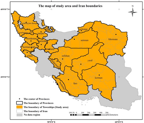
The study area is 18 provinces of Iran, in which the death rate of some cancers is registered by the Ministry of Health and Medical Education of Iran (MOH). The selected spatial unit is the township boundary. The number of townships in the study area is 192. Figure 1 shows the case study area.

Figure 1. Case study area of the research.

2.2. Design of the data framework and conceptual model

We first determined the causal parameters of skin cancer and then decided on representations for the necessary spatial and attribute data.

To do this, documents and reports from the World Health Organisation (WHO) and the MOH, the list of cancer-causing parameters published by the National Cancer Institute (NCI) of America, and other available documents were studied and discussed with experts on the subject. From these discussions, we determined that the most important parameters related to skin cancer include natural elements and climate, occupational and living environment (Pukkala et al. 2009), nutritional habits (Riboli 2013), and the usage of chemical fertilisers (Haffman 2007), which can be classified as environmental/climatic, social and economic parameters. Table 1 shows the summary of these factors and their spatial units.

Table 1. Causative factors of skin cancer and their spatial units.

Skin Cancer Causative Factors		Spatial Unit of Needed Data	Spatial Unit of Available Data	Used Attribute Data
Environmental and Climate Parameters	Solar Energy	Polygon	Point	11 year average of solar energy at measurement stations
	Hours of Sunshine and UV radiation	Polygon	Point	11 year average of hours of sunshine and UV radiation at measurement stations
	Air Humidity	Point	Average arsenic content in drinking water	Polygon
	Air Pressure	Point	Annual average air humidity at measurement stations	Polygon
	Air Temperature	Point	Annual average air pressure at measurement stations	Polygon
Parameters related to the environment of life and work	Contact with Tar	Polygon	Polygon	Number of workers that are in contact with tar
	Contact with Oil	Polygon	Polygon	Number of workers that are in contact with oil
	Contact with Coal	Polygon	Polygon	Number of workers that are in contact with coal
	Contact with Sun	Polygon	Polygon	Number of workers that are directly exposed to the sun in their occupations
Nutrition habits	Fruit and Vegetable Usage	Polygon	Polygon	Percentage of income that each family uses to buy fruit and vegetables
	Red Meat Usage			Percentage of income that each family uses to buy red meat
	Poultry Usage			Percentage of income that each family uses to buy poultry
	Sea food Usage			Percentage of income that each family uses to buy seafood
	Tobacco and Cigarette Usage			Percentage of income that each family uses to buy tobacco and cigarettes
Usage of chemical fertilisers for agriculture		Polygon	Polygon	Ratio of nitrogen, phosphoric, and potash as fertiliser in cultivated area

2.3. Data collection and processing

Based on the designed data framework and model requirements, interpolation methods and some spatial analysis, such as focal and overlay functions in a GIS environment, were used to prepare the raw spatial data. The following processes were carried out to prepare the data for entry into the model.

To consider the time variation in data and approximate them, a long-time average of causative factors is employed in this research. Actually, if a factor is problematic in long-time period its effect must be investigated in the infection of skin cancer. So in this research, the 11 years average of environmental and climatic parameters and 10 years average for other parameters are considered. The 11-year average was used because the sun’s activity has a period of 11 years (Hathaway 2010). Similar to the environmental and climatic parameters, for the other parameters the average values of the measurements in 10 years are calculated and attributed to the related townships. The reason for selecting of 10 years as the averaging period is that the effect of causative factors to infect the skin cancer is formed in a long time. Table 2 shows the time interval considered in this research.

Table 2. The considered time interval for causative factors in the model.

Factors	Time interval
Environmental and climatic parameters	11 years
Parameters related to environment of life and work	10 years
Nutrition habits	10 years
Usage of chemical fertilisers for agriculture	10 years

2.3.1. Environmental and climatic parameters

As discussed before, in this research, 11-year annual averages for the parameters of atmospheric pressure, temperature, humidity, solar energy, and bright sunshine hours were gathered for each township based on observations at existing climatologic stations and other resources. The averaging process was done using the following procedure:

• The average of the measurements of the above parameters was calculated for each observation station.

• A point layer was created for the observation stations, and the averages of the parameters were associated with their related points.

• Using the kriging method, a raster was created by interpolating the average values of the parameters between the stations. Kriging provides a solution to the problem of estimation based on a continuous model of stochastic spatial variation (Longley et al. 2015; Webster and Oliver 2007). It is preceded by an analysis of the spatial structure of the data (Wackernagel 2013). This statistical method provides an indication of the estimation error known as the kriging standard deviation, which is the square root of the kriging variance (Stein 1999). The inverse distance weighted (IDW) method was also used to assess climatic parameters. However, by selecting some control and check points, the results of the kriging method were found to be more acceptable than those of the IDW method.

  Figure 2. The maps of 11-yrars average of temperature, pressure, brightness sun shine hours, and humidity parameters.

  

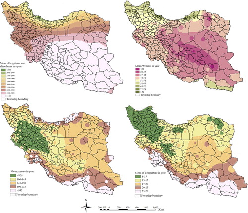
  Finally, the raster format of each parameter was overlaid with the polygon layer of the township boundaries. For each township, using focal analysis, the average of the raster cells inside township polygons is assumed to be the value of the parameter in that township. Figure 2 shows the maps produced for climatic parameters based on the 11-year averages.

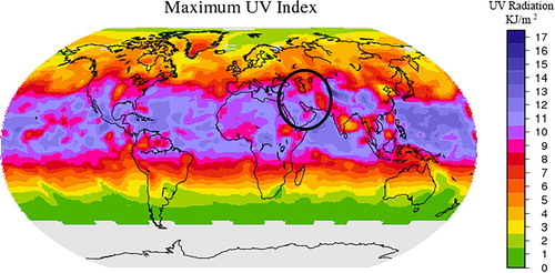
  Since one of the most important climatic parameters related to skin cancer is ultraviolet (UV) radiation (Lopo et al. 2014), in this research, the amount of UV radiation in Iran was investigated using data and maps from the ‘Longterm Multi-Sensoral UV Record’ project. This service provides long-term records of surface UV data based on several satellite instruments. As shown in Figure 3, the amount of radiation is approximately the same throughout the whole study area. Therefore, this factor was not imported into the model because this parameter does not vary among the spatial units.

2.3.2. Parameters related to the environment of life and work

According to the lists published by the US NCI and WHO and the reports and documents of the MOH, the following occupations reportedly have a higher than normal risk of skin cancer:

Figure 3. Long-term records of surface UV data produced by ‘Longterm Multi-Sensoral UV Record’ project.

• Occupations with high levels of sunlight exposure, such as farmers and fishermen.

• Occupations that allow for direct contact with tar, oil products, coal, and lead.

The International Standard Industrial Classification (ISIC) codes for mining, extraction, and production were used to define the relationship between these occupations and skin cancer. For example, for jobs related to coal, the following steps were taken:

• The ISIC codes for all occupations related to mining, production, and processing of coal were extracted.

• The number of people performing these jobs was calculated for each township and averaged over 10 years.

• This average was then associated with that township as the number of people dealing with coal.

In addition to the work environment, cancer-causing aspects of the living environment, including contamination of water and air, have been studied for decades (Skidmore 2002). Among other materials, radium and arsenic have been found to be related to several types of cancer, including skin cancer (Doyle and Wilkinson 2006). For these chemicals, the only data available for the whole country were polygon-based data on the arsenic content in drinking water resources. These data have been reported by the MOH in the township scale in Iran, which matches the resolution of our study.

2.3.3. Nutrition habits

Hospital-based case–control studies have found that several dietary factors are significantly associated with skin cancer (Elwood 2004). Moreover, according to WHO statistics, more than one-third of cancer deaths are related to diet. The only data available about dietary habits were the average annual family food budget, which is collected by the Statistical Centre of Iran (SCI). Studies have shown that the main diet-related factors associated with skin cancer include the consumption of fruit, vegetables, red meat, seafood, poultry, and tobacco (Calle et al. 2002; Prochaska et al. 2005). It is important to point out that the consumption of fruit, vegetables, seafood, and poultry decreases the risk of skin cancer, whereas the consumption of red meat and tobacco increases the risk.

2.3.4. Usage of chemical fertilisers for agriculture

The increase in the usage of chemical fertilisers has been proven to cause many diseases, including cancer, and other environmental problems (Lahans 2013). To include the effect of chemical fertilisers in the model, the usage of these materials for agriculture in the townships was entered into model.

2.4. Development Of the model

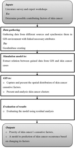
Based on the characteristics of the disease and the type of available data, a proper model should be specified. After this, the model should be calibrated using the data of both the response variable (here, skin cancer cases) and independent variables (here, the causative factors of skin cancer) (Armitage, Berry, and Matthewes 2010; Chun and Griffith 2013). Figure 4 shows the modelling process flow diagram.

Figure 4. The modelling process flow diagram.

2.4.1. Specification of the model

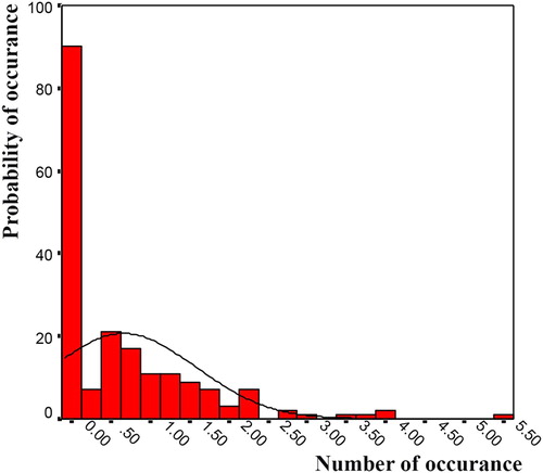
In this research, the generalised linear model (GLM) is used to define the relationship between skin cancer and its causative factors. The GLM is used for cases when the distribution function of the response variable is known and accepted with a high probability (Montgomery, Peck, and Vining 2012). The number of deaths by skin cancer, normalised by population, follows a Poisson distribution function with an acceptable probability. This is because the occurrence of death by cancer is binary. In addition, the probability of the disease occurring in high numbers is very low. These characteristics directly correspond with the Poisson function (Winkelmann 2013). Moreover, the correctness of the selection of the distribution function should be evaluated statistically. The fit of the selected function to the death data is evaluated by conducting the Kolmogorov–Smirnov test. Using this test, the probability distribution function of the deaths caused by skin cancer is determined to have a Poisson distribution with a probability of 97%. Figure 5 shows the chart of the distribution function of skin cancer data.

Figure 5. Chart of the distribution function of skin cancer data.

The GLM is actually an approach for unifying regression and experimental design models and unites the usual normal theory linear regression models and nonlinear models (Myers et al. 2010). A key assumption in the GLM is that the response variable distribution is a member of the exponential family of distributions (Hardin and Hible 2012; Montgomery, Peck, and Vining 2012; Piegorsch and Bailer 2005). This family includes the normal, binomial, Poisson, inverse normal, and gamma distributions. The general relation of the exponential family is shown in Equation (1).(1) $f(y_i,{\theta }_i,\mathrm{\Phi })=\exp \left\{\frac{[y_i{\theta }_i-b({\theta }_i\left)\right]}{a\left(\mathrm{\Phi }\right)+h(y_i,\mathrm{\Phi })}\right\}$(1)

In above relation, b(θ), a(Φ) and h(y, Φ) are the functions of known values, θ is the natural parameter of distribution function and Φ > 0 is the scale parameter of the function (Assuncao, Potter, and Cavenaghi 2002).

When the distribution function of the response variable is known and accepted with a high probability, a GLM can be used for simulation and modelling. In this research, the GLM is used to define the relationship between skin cancer and its causative factors because the number of deaths by skin cancer, normalised by population, follows a Poisson distribution function with an acceptable probability because of the occurrence of death by cancer is binary. In addition, the probability of the disease occurring in high numbers is very low. These characteristics directly correspond with the Poisson function (Winkelmann 2013). Moreover, the correctness of the selection of the distribution function can be evaluated statistically. When the distribution function is a Poisson distribution, Equation (1) converts to Equation (2) as follows:(2) $f(y_i,{\theta }_i,\mathrm{\Phi })=\exp \left\{[y_i\log (\mu )-\mu -\log (y_i!\left)\right]\right\}$(2) where μ is the mean value. Therefore, through comparison of Equation (1) and Equation (2), we can obtain Equation (3).(3) $\theta =\log \left(\mu \right),\varphi =1,a\left(\varphi \right)=1=\varphi ,b\left(\theta \right)=\mu =e^{\theta },h\left(y,\varphi \right)=-\log \left(y!\right)$(3)

There are three major elements in a GLM:

• Random element: In modelling one natural phenomenon, it is not possible to have access to a real model. Accordingly, the calculated model, when compared with the real model, always has observation and measurement errors. These errors are called the random elements of a GLM (Chun and Griffith 2013).

• Systematic element: In mathematics, when there is a relationship between two variables, this relationship is defined without any probability. For instance, Equation (4) shows the linear relation between response variable Y and dependent variable X. In this equation, β is the matrix of unknown coefficients (Atkinson and Riani 2002).(4) $Y=X_i\text{β}$(4)

However, when Equation (4) has any uncertainty, a random element enters the relationship. In Equation (5), ε is the random element.(5) $Y=X_i\text{β}+\epsilon$(5)

Thus, the part of the model that is accepted with 100% confidence is the systematic element.

• Link function: The basic idea of a GLM is the development of a linear model for an appropriate function of the expectation of the response variable. Let η_i be the linear predictor defined by Equation (6).(6) ${\eta }_i=g\left[E\right(y_i\left)\right]=g\left({\mu }_i\right)=x_i\text{β}$(6) where Y = [y₁, y₂, … , y_n] is the matrix of the response (dependent) variable, X = [x₁, x₂, … , x_n] is the matrix of the independent (regressor) variable, and β is the matrix of unknown coefficients (Lindsey 1997). Additionally, E(y_i) is driven according Equation (7).(7) $E\left(y_i\right)=g^{-1}\left({\eta }_i\right)=g^{-1}\left(x_i\text{β}\right)$(7) where g is called the link function (Rao et al. 2008). When the distribution function of the response variable is a Poisson distribution, the link function is logarithmic (Montgomery, Peck, and Vining 2012).

  Because evaluating all possible models can be computationally burdensome, various methods have been developed for evaluating only a small number of subset regression models by either adding or deleting regressors one at a time. Thus, we only examine models that fit well to the regressors (Miller, 2002). These methods are generally referred to as stepwise procedures. They can be classified into three broad categories: (1) forward selection, (2) backward elimination, and (3) stepwise regression (Lee et al. 2006; Rao et al. 2008). We now briefly describe and illustrate these procedures.

• Forward Selection: This procedure begins with the assumption that there are no regressors in the model other than the intercept. An effort is made to find an optimal subset by inserting regressors into the model one at a time. The first regressor selected for entry into the equation is the one that has the largest simple correlation with the response variable Y. Suppose that this regressor is $x_1$. This is also the regressor that will produce the largest value of the $F$ statistic for testing the significance of the regression. This regressor is entered if the $F$ statistic exceeds a preselected $F$ value, such as F_IN (or F_(to-entry)). The second regressor chosen is the one that now has the largest correlation with Y after adjusting for the effect of the first regressor ($x_1$) on Y. The procedure terminates either when the partial $F$ statistic at the particular step does not exceed F_IN or when the last candidate regressor is added to the model (Montgomery, Peck, and Vining 2012).

• Backward Elimination: Backward elimination attempts to find a good model by working in the opposite direction. This method starts a model with all of the candidates as predictors (Weiss 2005). The F statistic is then computed for each regressor as if it were the last variable to enter the model. The smallest of these F statistics is compared with a preselected value, F_out (or F_(to-remove)), for example, and if the smallest F value is less than F_out, that regressor is removed from the model. A regression model with K−1 regressors is then fit, the F statistics for this new model are calculated, and the procedure is repeated. The backward elimination algorithm terminates when the smallest F value is not less than the preselected cut-off value F_out.

• Stepwise Regression: The two procedures described above suggest a number of possible combinations. One of the most popular is the stepwise regression algorithm. Stepwise regression is the modification of forward selection in which all regressors entered into the model are reassessed via their F statistics. A regressor added at an earlier step may become redundant because of the relationships between it and the regressors now in the equation. If the F statistic for a variable is less than F_out, that variable is dropped from the model. Stepwise regression requires two cut-off values, F_IN and F_out. Some analysts prefer to choose F_IN – F_out, although this is not necessary. For large models and large data sets, stepwise procedures are a useful additional tool (Farhrmeir and Tutz 2013).

For the selection of the variables (causative factors) of skin cancer, the methods of forward selection, backward elimination, and stepwise selection were all used in this research, and the results are described in Results section.

2.4.2. Searching for interactive effects between variables

There are sometimes intrinsic correlations between variables. As mentioned by Rao et al. (2008), such correlations are mostly observed when researchers study natural phenomena with natural dependencies between parameters. Such correlations are called interactive effects. When two variables have an interactive effect, a change in one directly affects the other. Such interactive effects are represented in the model by a new variable that is the product of the two variables (Cohen et al. 2013; Montgomery, Peck, and Vining 2012).

2.4.3. Calculation of unknown coefficient

The common method for calculating unknown coefficients is the maximum likelihood estimation (MLE), which is described here. This approach considers l(β) to be the function that estimates the maximum probability, as shown in Equation (8).(8) $l\left(\text{β}\right)=\log \left[f\left(y,\theta ,\varphi \right)\right]=\log \left\{f\left[y,h\left(x\text{β}\right),\varphi \right]\right\}$(8) where θ = h(xβ). Furthermore, in Equation (9),(9) $U\left(\text{β}\right)=\frac{\mathrm{\partial }l\left(\text{β}\right)}{\mathrm{\partial }\text{β}}=\left[\begin{array}{c}\mathrm{\partial }l\left(\text{β}\right)/\mathrm{\partial }{\text{β}}_1\\ \mathrm{\partial }l\left(\text{β}\right)/\mathrm{\partial }{\text{β}}_2\\ ⋮\\ \mathrm{\partial }l\left(\text{β}\right)/\mathrm{\partial }{\text{β}}_p\end{array}\right]=\left[\begin{array}{c}{U}_1\left(\text{β}\right)\\ U_2\left(\text{β}\right)\\ ⋮\\ U_p\left(\text{β}\right)\end{array}\right].$(9) and in Equation (10),(10) $\begin{array}{rl}& A\left(\text{β}\right)=-\frac{{\mathrm{\partial }}^{2}l\left(\text{β}\right)}{\mathrm{\partial }{\text{β}}^t\mathrm{\partial }\text{β}}=-\frac{\mathrm{\partial }U\left(\text{β}\right)}{\mathrm{\partial }\text{β}}\\ & =\left[\begin{array}{cccc}\frac{-{\mathrm{\partial }}^{2}l\left(\text{β}\right)}{\mathrm{\partial }{\text{β}}_1\mathrm{\partial }{\text{β}}_1}& \frac{-{\mathrm{\partial }}^{2}l\left(\text{β}\right)}{\mathrm{\partial }{\text{β}}_1\mathrm{\partial }{\text{β}}_2}& \cdots & \frac{-{\mathrm{\partial }}^{2}l\left(\text{β}\right)}{\mathrm{\partial }{\text{β}}_1\mathrm{\partial }{\text{β}}_p}\\ \frac{-{\mathrm{\partial }}^{2}l\left(\text{β}\right)}{\mathrm{\partial }{\text{β}}_2\mathrm{\partial }{\text{β}}_1}& \frac{-{\mathrm{\partial }}^{2}l\left(\text{β}\right)}{\mathrm{\partial }{\text{β}}_2\mathrm{\partial }{\text{β}}_2}& \cdots & \frac{-{\mathrm{\partial }}^{2}l\left(\text{β}\right)}{\mathrm{\partial }{\text{β}}_2\mathrm{\partial }{\text{β}}_p}\\ ⋮& ⋮& \ddots & ⋮\\ \frac{-{\mathrm{\partial }}^{2}l\left(\text{β}\right)}{\mathrm{\partial }{\text{β}}_p\mathrm{\partial }{\text{β}}_1}& \frac{-{\mathrm{\partial }}^{2}l\left(\text{β}\right)}{\mathrm{\partial }{\text{β}}_p\mathrm{\partial }{\text{β}}_2}& \cdots & \frac{-{\mathrm{\partial }}^{2}l\left(\text{β}\right)}{\mathrm{\partial }{\text{β}}_p\mathrm{\partial }{\text{β}}_p}\end{array}\right]\\ & =\left[\begin{array}{cccc}{A}_{11}\left(\text{β}\right)& A_{12}\left(\text{β}\right)& \cdots & A_{1p}\left(\text{β}\right)\\ A_{21}\left(\text{β}\right)& A_{22}\left(\text{β}\right)& \cdots & A_{2p}\left(\text{β}\right)\\ ⋮& ⋮& \ddots & ⋮\\ A_{p1}\left(\text{β}\right)& A_{p2}\left(\text{β}\right)& \cdots & A_{pp}\left(\text{β}\right)\end{array}\right]\end{array}$(10)

If $\widehat{\text{β}}$ is the maximum likelihood estimate, then we obtain Equation (11).(11) $U\left(\widehat{\text{β}}\right)=0$(11)

Further, by the mean value theorem,(12) $-U\left({\text{β}}_0\right)=U\left(\widehat{\text{β}}\right)-U\left({\text{β}}_0\right)=\frac{\mathrm{\partial }U\left({\text{β}}^{\ast }\right)}{\mathrm{\partial }\text{β}}\left(\widehat{\text{β}}-{\text{β}}_0\right)=-A\left({\text{β}}^{\ast }\right)\left(\widehat{\text{β}}-{\text{β}}_0\right),$(12)

Thus, we obtain Equation (13).(13) $\widehat{\text{β}}-{\text{β}}_0=A^{-1}\left({\text{β}}^{\ast }\right)U\left({\text{β}}_0\right)\iff \widehat{\text{β}}={\text{β}}_0+A^{-1}\left({\text{β}}^{\ast }\right)U\left({\text{β}}_0\right).$(13)

Motivated by the last equation, two algorithms can be used to obtain the maximum likelihood estimate $\widehat{\text{β}}$;

1. Newton–Raphson method, shown in Equation (14):(14) $\begin{array}{rl}& {\widehat{\text{β}}}_{t+1}={\widehat{\text{β}}}_t+A^{-1}\left({\widehat{\text{β}}}_t\right)U\left({\widehat{\text{β}}}_t\right)\\ & \iff A\left({\widehat{\text{β}}}_t\right){\widehat{\text{β}}}_{t+1}=A\left({\widehat{\text{β}}}_t\right){\widehat{\text{β}}}_t+U\left({\widehat{\text{β}}}_t\right),t=0,1,2,\dots \end{array}$(14)

2. Fisher’s scoring method, shown in Equation (15):(15) $\begin{array}{rl}& {\widehat{\text{β}}}_{t+1}={\widehat{\text{β}}}_t+I^{-1}\left({\widehat{\text{β}}}_t\right)U\left({\widehat{\text{β}}}_t\right)\\ & \iff I\left({\widehat{\text{β}}}_t\right){\widehat{\text{β}}}_{t+1}=I\left({\widehat{\text{β}}}_t\right){\widehat{\text{β}}}_t+U\left({\widehat{\text{β}}}_t\right),t=0,1,2,\dots \end{array}$(15)

The above two algorithms will stop when $\left|U\left({\widehat{\text{β}}}_N\right)\right|<\epsilon$ or $\left|{\widehat{\text{β}}}_{N+1}-{\widehat{\text{β}}}_N\right|<\epsilon$, where ε is some prespecified small number.

2.4.4. Analysing of residuals

In any model fitting procedure, the analysis of the residuals is important in fitting the GLM. Residuals can provide guidance concerning the overall adequacy of the model, assist in verifying assumptions, and indicate the appropriateness of the selected link function (Myers et al. 2010).

It is generally recommended that residual analysis in the GLM be performed using deviance residuals. As shown in Equation (8), the ith deviance residual is defined as the square root of the contribution of the ith observation to the deviance, multiplied by the sign of the raw residual, as shown in Equation (16).(16) $r_{p_i}=\sqrt{d_i}\mathrm{s}\mathrm{i}\mathrm{g}\mathrm{n}(y_i-{\hat{y}}_i)$(16) where $d_i$ is the contribution of the ith observation to the deviance (Montgomery, Peck, and Vining 2012). For the Poisson distribution with the log link function, the deviance gives the log likelihood ratio statistic for the contingency tables (Lindsey 1997).

In this research, the deviance residuals were calculated for three methods of stepwise regression, and the results are presented in the Results section.

2.4.5. Calibration of the model

The data of both the disease and its causative factors were entered into the statistical model. As a result, a statistical formula was generated, in which the statistically significant parameters are defined along with the coefficients related to each parameter. In addition, statistical values are provided showing the significance of each parameter in the disease’s model.

The degree of freedom in the model is 163 because the research was performed in 18 provinces of Iran with 192 townships.

Because evaluating all possible models can be computationally burdensome, various methods have been developed for evaluating only a small number of subset regression models by either adding or deleting regressors one at a time. Thus, we will only examine models that fit well with the regressors (Miller, 2002). using the three broad methods described before: (1) forward selection, (2) backward elimination, and (3) stepwise regression (Lee et al. 2006; Rao et al. 2008). For the selection of the variables (causative factors) of skin cancer, the methods of forward selection, backward elimination, and stepwise selection were all used. Moreover, interactive effects between variables have been assessed.

3. Results and Discussion

The parameters that resulted from each method, in order of significance, are as follows:

• In the forward selection method: temperature, pressure, interactive effect of bright sunshine hours and solar energy, solar energy, bright sunshine hours, number of farmers, and contact with lead;

• In the backward elimination method: temperature, pressure, interactive effect of bright sunshine hours and solar energy, solar energy, bright sunshine hours, contact with lead, number of farmers, fruit and vegetable consumption, phosphate fertiliser usage, and tobacco consumption;

• In the stepwise selection method: temperature, pressure, interactive effect of bright sunshine hours and solar energy, solar energy, bright sunshine hours, number of farmers, fruit and vegetable consumption, contact with lead, potassium fertiliser usage, tobacco consumption.

These models can be compared based on their deviance values. As shown in Table 3, the deviance value related to the stepwise method is lower than the deviance values related to the other two methods. Therefore, the model using the stepwise method model is accepted as the model representing the spatial distribution of skin cancer in the study area. Table 3 shows comparisons between the deviance residual of the models based on the selected method.

Table 3. Comparison between deviance residual of parameter selection methods.

Method of parameter selection	Acceptance level of deviance	Test result
Forward selection	141.3549	Accepted
Backward elimination	139.6979	Accepted
Stepwise selection	138.7203	Accepted

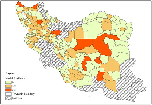
Figure 6 shows the deviance residuals of the three selection methods; forward, backward, and stepwise selection. Figures 6.1, 6.2, and 6.3 show that the deviance residuals related to the model using the stepwise selection method are smaller than those of the two other models. The residuals for the model generated by the stepwise selection method are shown in the map in Figure 7. This map shows the difference between the values predicted by the model and the real values of the disease cases. The map shows that higher residuals occur in the areas where the disease counts are much higher or much lower than the rest of the study area. This occurs because the model should fit and pass through all variations of values in the best possible way. With such an approach, the extreme values are moderated.

Figure 6. Chart showing the deviance residuals of the 3 regression methods (6.1. stepwise method, 6.2. backward elimination method, and 6.3. forward selection method).

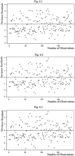
Figure 7. Map of the residuals in the stepwise approach.

The main causative factors of skin cancer are extracted using the stepwise method because of its lower residual. Equation (18) shows the statistical relationship between skin cancer and its causative factors that results from stepwise selection. Notably, in the statistical relations, the residuals are defined and can be analysed.(18) $\begin{array}{rl}f\left(y\right)& =[\exp \left(\right(+0.2265\ast \mathrm{P}23)+0.1809)\\ & \times \exp \left(\right(-0.0014\ast \mathrm{P}25)-0.3410)\\ & \times \exp \left(\right(+7.4349\ast \mathrm{P}15)-0.8563)\\ & \times \exp \left(\right(+0.0083\ast \mathrm{P}24)-0.9374)\\ & \times \exp \left(\right(+137.0906\ast \mathrm{P}1)-0.1012)\\ & \times \exp \left(\right(-0.00000134\ast \mathrm{P}18)+0.0061)\\ & \times \exp \left(\right(+111.2446\ast \mathrm{P}14)+0.0204)\\ & \times \exp \left(\right(+0.00002504\ast \mathrm{P}6)-0.0056)\\ & \times \exp \left(\right(+0.000005914\ast \mathrm{P}17)+0.0051)]\\ & /\exp \left(\right(-0.00244\ast \mathrm{P}15\ast \mathrm{P}24)+0.8667)\$\end{array}$(18)

In which, f(y) is the number of skin cancer occurrences and P_i is the causative factor, as described in Table 4. As shown in Table 4, some parameters have positive coefficients, which indicate a positive relationship between that parameter and skin cancer. In contrast, parameters with negative coefficients exhibit a negative relationship with skin cancer. The factors P18, P6 and P17 in Equation (18) appear to be quite insignificant as their coefficients are remarkably low. However, the insignificance of these factors was realised only after the implementation of the research. Therefore, as part of the research results, they are worth mentioning. On the other hand, from a pragmatic point of view, when using Equation (18), these factors can be removed from the equation.

Table 4. Variables that emerged in the model along with their positive/negative sign in the model.

Variable description	The name of Parameter in Equation 18	Sign of coefficient
Number of farmers per township population	P1	Positive
Usage of potassium fertiliser in cultivated area	P6	Positive
Number of factory workers in contact with lead per township population	P14	Positive
Solar energy per area unit	P15	Positive
Average smoking expenses per family	P17	Positive
Average fruit/vegetable expenses per family	P18	Negative
Annual average temperature	P23	Positive
Annual bright sunshine hours	P24	Positive
Annual average atmosphere pressure	P25	Negative
Interactive effect of annual hours of sunlight and solar energy	P15*P24	Negative

The above model describes the relationship between the disease counts per spatial unit and the measured value of the parameters, with each represented by a variable. Therefore, the model can be used to estimate the disease counts under different scenarios. Such a scenario could be the result of changes in the parameters made either naturally or by the decisions of welfare managers.

Before changing any of the parameters, the estimated occurrences of cancer for all townships are calculated using the formula of the model. These estimated values are certainly different from the observed (reported) values. However, to realise the effect of any change in a parameter, the estimated values calculated from the formula, rather than the real occurrence values, should be used.

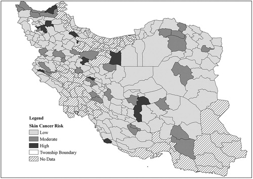
The resulting estimated (calculated) cancer occurrences for all townships are shown in Figure 8. The map shows the probability mapping of the calculated cancer occurrences. Probability mapping is a geo-statistical approach for the visualisation of polygon-based disease statistics. A description of this approach, along with its advantages and reasons for using it, can be found in Cromley and McLafferty (2012). It should be mentioned that in Figure 8, the classification to show the risk levels is as below:

Figure 8. The probability mapping of skin cancer occurrences calculated from the model.

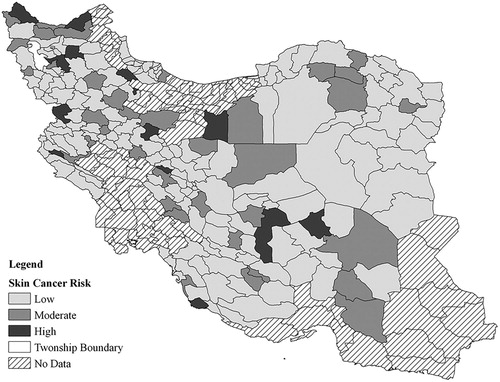
• 0–5 mortality cases: Low risk

• 5–10 mortality cases: Moderate risk

• More than 10 cases: High risk

We have based this classification on the informed opinion of cancer researchers, and we think the rates are not applicable to other parts of world, as the risk depends on the rate of mortality in a region.

To show the predictive ability of the model, we assume a case where, as a result of public education and encouragement, the consumption of fruits and vegetables increases by 20% as a scenario in the model. To represent this change, the values of fruit and vegetable consumption are increased by 20% in all townships in the study area. The values of all parameters, including the changed values, are then entered into the model formula, and the new disease occurrences are calculated for all townships. The new values for cancer occurrence are again mapped using the probability mapping approach. The results are shown in Figure 9. For ease of comparison, the risk levels in this figure are defined the same with Figure 8. Obviously, in many of the townships, the disease count is reduced and the disease crisis is improved, showing the effect of the 20% increase in fruit and vegetable consumption.

Figure 9. The probability mapping of skin cancer occurrences calculated from the model, with the consumption of fruits and vegetables increased by 20%.

Because of the large number of townships, changes in the disease counts of the individual townships are not reported. However, after introducing a 20% increase in fruit and vegetable consumption, the average cancer occurrences per township decreased by 8%. Figures 8 and 9 illustrate this change in the model.

4. Conclusions

In this research, the occurrence of skin cancer is modelled using its main causative factors employing the GLM. This model can be used in monitoring and predicting factors that cause skin cancer. Hence, the Digital Earth concept, using the interdisciplinary themes of (i) climatic parameters, such as temperature, hours of sunshine, and rainfall, (ii) geospatial technologies, (iii) environmental parameters, such as relief, geostatistical data and models, and medical data, has been shown to be a valuable approach to studying global diseases such as skin cancer and can be used in all affected countries around the world. The main conclusions from this study can be summarised as follows:

• As was expected due to its flexibility, the stepwise selection approach showed better results than the other methods. An advantage of this method is that the significance of parameters relative to each other and their relationships are studied and considered better than in the other methods. The disadvantage of this method is that when the number of parameters is large, the procedure of entering and removing parameters is complex and time consuming.

• The main parameters causing or affecting skin cancer, in order of significance, are temperature, atmospheric pressure, the interactive effect of bright sunshine hours and solar energy, solar energy, bright sunshine hours, the number of farmers, fruit and vegetable consumption, contact with lead, potassium fertiliser usage, and tobacco consumption.

• Unexpectedly, the climatic parameters all have significant roles in the model when combined with each other. This means that the removal of any one parameter causes the others to also be removed from the model, and the residuals increase greatly.

• The accuracy of the model depends strongly on the accuracy of the input data. A change in any of the parameters causes a change in the model in proportion to the significance of that parameter in the model. Therefore, in the next round of modelling, the parameter data, including both spatial and attribute data, should be collected more carefully and more accurately.

• Thus, geospatial technology, using the Digital Earth approach, enables better-informed decision-making by providing improved national statistics on skin cancer and by ensuring that the skin cancer data are geospatially explicit.

Disclosure statement

No potential conflict of interest was reported by the authors.

References

- Anderson, K., R. Barbara, S. William, K. Argyro, and F. Lawrence. 2017. “Earth Observation in Service of the 2030 Agenda for Sustainable Development.” Geo-spatial Information Science 20 (2): 77–96. doi:10.1080/10095020.2017.1333230.
- Anthamatten, P., and H. Hazen. 2011. An Introduction to the Geography of Health. New York: Routledge.
- Apalla, Zoe, Aimilios Lallas, Elena Sotiriou, Elizabeth Lazaridou, and Demetrios Ioannides. 2017. “Epidemiological Trends in Skin Cancer.” Dermatology Practical & Conceptual 7 (2): 1–6. PMC. Web. 18 June 2018. doi: 10.5826/dpc.0702a01
- Armitage, P., G. G. Berry, and J. N. S. Matthewes. 2010. Statistical Methods in Medical Research. 4th ed. Blackwell: Oxford, 357.
- Assuncao, R. M., J. E. Potter, and S. M. Cavenaghi. 2002. “A Bayesian Space Varying Parameter Model Applied to Estimating Fertility Schedules.” Statistics in Medicine 21 (4): 2057–2075. doi: 10.1002/sim.1153
- Atkinson, A., and M. Riani. 2002. Robust Diagnostic Regression Analysis. New York, USA: Springer, 16–18.
- Bermudez, L. 2017. “New Frontiers on Open Standards for Geo-Spatial Science.” Geo-spatial Information Science 20 (2): 126–133. doi: 10.1080/10095020.2017.1325613
- Bristow, R. E., J. Chang, A. Ziogas, D. L. Gillen, L. Bai, and V. M. Vieira. 2015. “Spatial Analysis of Advanced-Stage Ovarian Cancer Mortality in California.” American Journal of Obstetrics and Gynecology 213 (1): 43.e1–43.e8. doi:10.1016/j.ajog.2015.01.045.
- Calle, E. E., C. Rodriguez, E. J. Jacobs, M. L. Almon, A. Chao, M. L. McCullough, H. S. Feigelson, and M. J. Thun. 2002. “The American Cancer Society Cancer Prevention Study II Nutrition Cohort: Rationale, Study Design, and Baseline Characteristics.” Cancer 15; 94 (2): 500–511. doi: 10.1002/cncr.10197
- Chun, Y., and D. A. Griffith. 2013. Spatial Statistics and Geostatistics: Theory and Applications for Geographic Information Science. Thousand Oaks, CA: SAGE.
- Cohen, J., P. Cohen, S. G. West, and L. S. Aiken. 2013. Applied Multiple Regression Correlation Analyses for the Behaviour Sciences. 3rd ed, 64–99. London: Routledge.
- Cromley, E. K., and S. L. McLafferty. 2012. GIS and Public Health. 2nd ed, 133–157. New York: The Guilford Press.
- Croner, C. M., J. Sperling, and F. R. Broome. 1996. “Geographic Information Systems (GIS): New Perspectives in Understanding Human Health and Environmental Relationships.” Statistics in Medicine 15 (18): 1961–1977. doi: 10.1002/(SICI)1097-0258(19960930)15:18<1961::AID-SIM408>3.0.CO;2-L
- Davis, J. M., and Y. Garb. 2018. “A Strong Spatial Association between e-Waste Burn Sites and Childhood Lymphoma in the West Bank, Palestine.” International Journal of Cancer 6 (1).
- Doyle, P., and P. Wilkinson. 2006. “Radiation and Hazardous Waste: Ionizing Radiation.” In Environmental Epidemiology: Understanding Public Health, edited by P. Wilkinson, 69–80. London: Open University Press.
- Elwood, M. 2004. “Who Gets Skin Cancer: Individual Risk Factors?” In Prevention of Skin Cancer, edited by D. Hill, M. Elwood, and D. R. English, 3–20. Berlin: Springer.
- Farhrmeir, L., and G. Tutz. 2013. Multivariate Statistical Modeling Based on Generalized Linear Models. 2nd ed, 140–145. New York, USA: Spinger.
- Forbes, H., and E. Watt. 2015. Jarvis’s Physical Examination and Health Assessment. 2nd ed, 830. Melbourne: Elsevier Publications.
- Fradelos, E. C., I. V. Papathanasiou, D. Mitsi, K. Tsaras, C. F. Kleisiaris, and L. Kourkouta. 2014. “Health Based Geographic Information Systems (GIS) and Their Applications.” Acta Informatica Medica 22 (6): 402–405. doi:10.5455/aim.2014.22.402-405.
- Glass, G. E. 2000. “Geographic Information Systems.” In Infectious Disease Epidemiology: Theory and Practice, edited by K. Nelson and C. Williams, 231–254. Gaithersburg, MD: Apsen Publishers Inc.
- Guest, G. 2015. “Introduction to Public Health Research Methods.” In Public Health Research Methods, edited by G. Guest, and E. E. Namey, 1–30. London: SAGE Publications.
- Haffman, E. J. 2007. Cancer and the Search for Selective Biochemical Inhibitors. New York: CRC Press.
- Hardin, J. W., and J. M. Hible. 2012. Generalized Linear Models and Extensions, 7–13. Lubbock, TX: Sata Press.
- Hathaway, D. H. 2010. “The Solar Cycle.” Living Reviews in Solar Physics 7 (1): 6–65. doi: 10.12942/lrsp-2010-1
- Kelsall, J., and J. Wakefield. 2002. “Modeling Spatial Variation in Disease Risk: a Geostatistical Approach.” Journal of the American Statistical Association 97 (459): 692–701. doi: 10.1198/016214502388618438
- Kurland, K. S., and W. Gorr. 2014. GIS Tutorial for Health. 5th ed. New York, USA: ESRI press.
- Lahans, T. 2013. The Geology of the Modern Cancer Epidemic: Through the Lens of Chinese Medicine. London: World Scientific.
- Lee, Y., J. Nelder, Y. Pawitan, N. Reid, S. Murphy, R. Tibshirani, T. Louis, H. Tong, N. Keiding, and V. Isham. 2006. Generalized Linear Models with Random Effects. New York: Chapman and Hall/CRC.
- Lindsey, J. K. 1997. Applying Generalized Linear Models, 210–211. New York, USA: Springer.
- Longley, P. A., M. F. Goodchild, D. J. Maguire, and D. W. Rhind. 2015. Geographic Information Systems and Science. 4th ed. Hoboken, NJ: Wiley Publication.
- Lopo, A. B., M. H. Spyrides, P. S. Lucio, and J. Sigró. 2014. “UV Index Modeling by Autoregressive Distributed lag (ADL Model.” Atmospheric and Climate Sciences 4: 323–333. doi: 10.4236/acs.2014.42033
- MacKinnon, J. A., R. C. Duncan, Y. Huang, D. J. Lee, L. E. Fleming, L. Voti, M. Rudolph, and D. Wilkinson. 2007. “Detecting an Association Between Socioeconomic Status and Late Stage Breast Cancer Using Spatial Analysis and Area-Based Measures.” Cancer Epidemiology Biomarkers and Prevention 16 (4): 756–762. doi: 10.1158/1055-9965.EPI-06-0392
- Mahesvaran, R., and R. P. Haining. 2016. “Disease Mapping and Spatial Analysis.” In GIS in Public Health Practice, edited by R. Mahesvaran, and M. Craglia, 13–30. New York: CRC press.
- Mansour, S. 2016. “Spatial Analysis of Public Health Facilities in Riyadh Governorate, Saudi Arabia: A GIS-Based Study to Assess Geographic Variations of Service Provision and Accessibility.” Geo-Spatial Information Science 19 (1): 26–38. doi: 10.1080/10095020.2016.1151205
- Melnick, A. L. 2002. Introduction to Geographic Information Systems in Public Health, 61–62. Gaithersburg, Maryland: Aspen Publishers.
- Mesgari, M. S., and Z. Masoomi. 2008. “GIS Applications in Public Health as a Decision Making Support System and It’s Limitation in Iran.” World Applied Sciences Journal 3 (1): 73–77.
- Miller, A. J. 2002. Subset Selection in Regression, 39–46. Washington, DC: CRC Press.
- Mohebbipour, A., S. Alipour, S. Sadeghiyeh, F. Amani, and E. Farzaneh. 2015. “Investigating the Geographical Distribution of Skin Cancer (BCC Type) in Ardabil Province via GIS.” International Journal of Research in Medical Sciences 3 (8): 2093–2098. doi: 10.18203/2320-6012.ijrms20150332
- Moncrieff, S., G. West, J. Cosford, N. Mullan, and A. Jardine. 2014. “An Open Source, Server-Side Framework for Analytical web Mapping and its Application to Health.” International Journal of Digital Earth 7 (4): 294–315. doi: 10.1080/17538947.2013.786143
- Montgomery, D., E. Peck, and G. Vining. 2012. Introduction to Linear Regression Analysis. 5th ed, 466–487. New York: Wiley Interscience Publication.
- Musa, G. J., P. H. Chiang, T. Sylk, R. Bavley, W. Keating, B. Lakew, H. C. Sou, and C. W. Hoven. 2013. “Use of GIS Mapping as a Public Health Tool—From Cholera to Cancer.” Health Service Insights 6: 111–116. doi: 10.4137/HSI.S10471
- Myers, R. H., D. C. Montgomery, G. G. Vining, and T. J. Robinson. 2010. Generalized Linear Models: with Applications in Engineering and the Sciences. 2nd ed. Hoboken, NJ: John Willey and Sons.
- O’Hanlon, S. J., H. C. Slater, R. A. Cheke, B. A. Boatin, L. E. Coffeng, S. D. Pion, M. Boussinesq, H. G. M. Zouré, W. A. Stolk, and M. G. Basáñez. 2016. “Model-Based Geostatistical Mapping of the Prevalence of Onchocerca Volvulus in West Africa.” Neglected Tropical Disease 10 (1): 1–36.
- Pakzad, R., M. Ghoncheh, Z. Pournamdar, Pakzad I. Momenimovahed, H. Salehiniya, F. Towhidi, and B. R. Makhsosi. 2016. “Spatial Analysis of Skin Cancer Incidence in Iran.” Asian Pacific Journal of Cancer Prevention, Cancer Control in Western Asia 17 ( Special Issue): 33–37. doi: 10.7314/APJCP.2016.17.S3.33
- Piegorsch, W. W., and A. J. Bailer. 2005. Analysing Environmental Data, 104–105. Sussex: John Wiley and Sons.
- Prochaska, J. O., W. F. Velicer, C. Redding, J. S. Rossi, M. Goldstein, J. DePue, G. W. Greene, et al. 2005. “Stage-based Expert Systems to Guide a Population of Primary Care Patients to Quit Smoking, Eat Healthier, Prevent Skin Cancer, and Receive Regular Mammograms.” Preventive Medicine 41 (2): 406–416. doi: 10.1016/j.ypmed.2004.09.050
- Pukkala, E., J. I. Martinsen, E. Lynge, H. K. Gunnarsdottir, P. Sparén, L. Tryggvadottir, E. Weiderpass, and K. Kjaerheim. 2009. “Occupation and Cancer – Follow-up of 15 Million People in Five Nordic Countries.” Acta Oncologica 48 (5): 646–790. doi:10.1080/02841860902913546.
- Rao, C. R., H. Toutenburg, C. Shalabh, and C. Heumann. 2008. Linear Models and Generalizations: Least Squares and Alternatives, 164–394. New York: Springer.
- Razi, S., M. Enayatrad, A. Mohammadian-Hafshejani, H. Salehiniya, M. Fathali-loy-dizaji, and S. Soltani. 2015. “The Epidemiology of Skin Cancer and its Trend in Iran.” International Journal of Preventive Medicine 6 (1): 64.
- Riboli, E. 2013. “The Role of Metabolic Carcinogenesis in Cancer Causation and Prevention Into Cancer From the European Perspective Investigation Into Cancer and Nutrition.” In Advances in Nutrition and Cancer, edited by V. Zappia, S. Panico, G. L. Russo, A. Budillon, and F. D. Ragione. Berlin: Springer Science & Business Media.
- Sarfraz, M. S., N. K. Tripathi, and A. Kitamoto. 2014. “Near Real-Time Characterisation of Urban Environments: a Holistic Approach for Monitoring Dengue Fever Risk Areas.” International Journal of Digital Earth 7 (11): 916–934. doi: 10.1080/17538947.2013.786144
- Schura, N., E. Hürlimanna, A. S. Stensgaardd, K. Chimfwembef, G. Mushingef, C. Simoongag, N. Kabatereineh, T. Kristensene, J. Utzingera, and P. Vounatsoua. 2013. “Spatially Explicit Schistosoma Infection Risk in Eastern Africa Using Bayesian Geostatistical Modelling.” Acta Tropica 128: 365–377. doi: 10.1016/j.actatropica.2011.10.006
- Schwartz, G. G., and C. L. Hanchette. 2006. “UV, Latitude, and Spatial Trends in Prostate Cancer Mortality: All Sunlight is Not the Same (United States).” Cancer Causes & Control 17: 1091–1101. doi: 10.1007/s10552-006-0050-6
- Scott, G., and A. Rajabifard. 2017. “Sustainable Development and Geospatial Information: A Strategic Framework for Integrating a Global Policy Agenda Into National Geospatial Capabilities.” Geo-spatial Information Science 20 (2): 59–76. doi: 10.1080/10095020.2017.1325594
- Siangphoe, U., and D. C. Wheeler. 2016. “Modelling Spatial Variation in Disease Risk in Epidemiologic Studies.” In Spatial Analysis in Health Geography, edited by P. Kanaroglou, E. Delmelle, and A. Paez, 121–136. New York: Routledge.
- Skidmore, A. 2002. Environmental Modeling with GIS and Remote Sensing, 8–55. London: Taylor & Francis.
- Stein, M. L. 1999. Interpolation of Spatial Data: Some Theory for Kriging, 8–10. New York: Springer.
- Tian, N., J. Wilson, and F. Zhan. 2011. “Spatial Association of Racial/Ethnic Disparities between Late-Stage Diagnosis and Mortality for Female Breast Cancer: Where to Intervene?” International Journal of Health Geographics 10 (24): 1–9.
- van Genderen, J. L. 2017. “Perspectives on the Nature of Geospatial Information.” Geo-Spatial Information Science 20 (2): 57–58. doi:10.1080.10095020.2017.1337320 doi: 10.1080/10095020.2017.1337320
- Vieira, V. M., C. Villanueva, J. Chang, A. Ziogas, and R. E. Bristow. 2017. “Impact of Community Disadvantage and air Pollution Burden on Geographic Disparities of Ovarian Cancer Survival in California.” Environmental Research 156: 388–393. doi: 10.1016/j.envres.2017.03.057
- Wackernagel, H. 2013. Multivariate Geostatistics: An Introduction with Applications. 2nd ed, 96–99. Berlin: Springer.
- Wartenberg, D. 1993. “Identification and Characterization of Populations Living Near High-Voltage Transmission Lines: A Pilot Study.” Environmental Health Perspectives 101: 626–632. doi: 10.1289/ehp.93101626
- Webster, R., and M. A. Oliver. 2007. Geostatistics for Environmental Scientists, 154–155. Chichester: John Wiley and Sons.
- Weiss, R. E. 2005. Modeling Longitudinal Data, 151–152. New York, USA: Springer.
- Wertheimer, N., and E. Leeper. 1979. “Electric Wiring Configuration and Childhood Cancer.” American Journal of Epidemiology 109: 273–284. doi: 10.1093/oxfordjournals.aje.a112681
- Wheeler, B. W., G. Kothencz1, and A. S. Pollard. 2013. “Geography of Non-Melanoma Skin Cancer and Ecological Associations with Environmental Risk Factors in England.” British Journal of Cancer 109: 235–241. doi: 10.1038/bjc.2013.288
- Winkelmann, R. 2013. Econometric Analysis of Count Data. 2nd ed, 8–10. New York, USA: Springer.
- Wu, K., X. Huo, and G. Zhu. 2008. “Relationships between Esophageal Cancer and Spatial Environment Factors by Using Geographic Information System.” Science of the Total Environment 393 (2–3): 219–225. doi: 10.1016/j.scitotenv.2007.12.029
- Yomralioglu, T., E. Colak, and A. C. Aydinoglu. 2009. “Geo-Relationship Between Cancer Cases and the Environment by GIS: A Case Study of Trabzon in Turkey.” International Journal of Environmental Research and Public Health 6: 3190–3204. doi: 10.3390/ijerph6123190