Analysis of dependence of grey wolf optimizer to shift-transformations and its shift-invariant improved methods adaptively controlling the search areas

ABSTRACT

As a metaheuristic method for the continuous optimization problem, the grey wolf optimizer (GWO) has attracted much attention from researchers because the method is reported to be superior to other methods. However, some works show that the GWO is too specialized only to problems having the zero-optimal solution, which can lead to a significant deterioration of the efficiency for other problems. In this paper, we, first, theoretically prove the shift-dependence of the GWO, which is the underlying cause of the over-specialization of the GWO, and we experimentally analyze the property by using a larger number of problems. Secondly, we propose am shift-invariant GWO, GWO-SR, and, modify the GWO-SR by adding two methods: an adjustment technique the size of the search area and a mutation process to enhance the diversity of the search (GWO-AS) Finally, we show advantages of two proposed GWOs by comparing them with other metaheuristic methods.

KEYWORDS:

• Grey wolf optimizer
• global optimization
• shift-invariance
• reference point
• control of the sizes of search areas
• metaheuristics

1. Introduction

The grey wolf optimizer (GWO) is one of the nature-inspired metaheuristic methods which exploits hunting techniques and social hierarchy of the grey wolves in order to solve global optimization problems [1, 2]. The GWO has attracted significant attention from researchers because the method has been reported to have high performance in seeking high-quality solutions regardless its simple algorithm according to many studies [3–8], and thus, it has been applied to a wide range of fields [9–12].

However, a previous work [13] shows that the GWO is not invariant to shift-transformations in the orthogonal coordinate representation of the optimization problem. In addition, the some works [14, 15] show that the performance of the GWO is often considerably low when the optimal solution is far from the origin. In addition, a work [16] showed that the search behavior of the GWO is too specialized for problems having the optimal solution at the origin through numerical experiments, and that the updating systems of the GWO widely depend on the distance of the origin to the best solution found so far. The property can lead to a significant deterioration of the efficiency of the search process for other problems whose optimal solution is not the origin. Thus, many improved GWOs, which have been investigated [3–8], can have the same drawbacks if its updating systems are not shift-invariant similar to the original GWO. Furthermore, in the work, authors proposed a shift-invariant method GWO with reference points (GWO-R) to overcome the drawback, in which grey wolves are updated by shift-invariant systems exploiting the reference points instead of the origin.

In this paper, we first analyze the underlying causes of too specialized properties of the GWO in more detail. We theoretically show that the GWO is not invariant to shift-transformations, and experimentally clarify ineffective search of the GWO due to the property by using more shifted problems than in work [16]. These results show that the performance evaluations of the GWO in many studies are not fair for a general-purpose metaheuristic method for global optimization problems.

Secondly, we propose a modified GWO-R, GWO-SR, to improve the insufficient intensive search of GWO-R in the final stages, in which the size of search areas are adjusted more reasonably with respect to the distance between the reference point and the best solutions. Then, we experimentally show that the search is effective if the reference point is chosen appropriately. Moreover, we improve the GWO-SR by adding an adjusting method of search areas and a mutation process in order to strengthen the diversity of the search, which is called the GWO with adjustment of the search area (GWO-AS). Finally, we show the good performance of the proposed GWOs, GWO-SR and GWO-AS, by comparing them with other metaheuristic methods such as particle swarm optimization (PSO) [17, 18] and firefly algorithm (FA) [19, 20].

This paper is organized as follows. In Section 2, we introduce the GWO, and in Section 3, we analyze the property of its search process, and point out the shift-dependence and the over-specialization of its search process. In Sections 4 and 5, we propose new modified GWOs exploiting a reference point or an adjustment of search area and a mutation process, which overcome the above drawbacks. In Section 6, through numerical experiments, we verify the effectiveness of the proposed methods. Finally, we conclude this paper in Section 7.

2. Grey wolf optimizer

The GWO is one of metaheuristic methods for continuous global optimization, in which the hunting technique and the social hierarchy of grey wolves are mathematically exploited in order to solve global optimization problems [1, 2]. Regardless of its simple algorithm, the GWO is reported to have a high performance of finding desirable solutions of the optimization. In this section, we introduce the standard GWO.

Throughout this paper, we mainly consider the following continuous optimization problems having many local minima and the rectangular constraint. $\begin{array}{r}\text{(P1)}\underset{\mathit{x}}{\text{min}}f\left(\mathit{x}\right)\text{s.t.}\mathit{x}\in X:=\prod _{j=1}^n[x_j^l,x_j^u].\end{array}$Here, $f:{\mathrm{\Re }}^n\to \mathrm{\Re }$ denotes the objective function to be minimized, and X $\subset {\mathrm{\Re }}^n$ does the feasible region. In order to solve the problem, the GWO uses a number of search agents called grey wolves. The position of each grey wolf i, $i\in W$ denotes a candidate solution of the problem, which are represented as ${\mathit{x}}^{\left(i\right)}\left(t\right)$ $\in {\mathrm{\Re }}^n$ at iteration t, where W denotes an index set of all grey wolves. These positions are updated in a way that models the social hierarchy and tracking, encircling, and attacking a prey of the grey wolves as follows: (1) $\begin{array}{rl}& {\mathit{d}}^{(p,i)}\left(t\right):=|2{\mathit{r}}^{(p,1)}\otimes {\mathit{x}}^{\left(p\right)}(t)-{\mathit{x}}^{\left(i\right)}(t\left)\right|,\end{array}$(1) (2) $\begin{array}{rl}& \mathrm{\Delta }{\mathit{x}}^{(p,i)}\left(t\right):=\mathit{a}\left(t\right)\otimes (2{\mathit{r}}^{(p,2)}-\mathbf{1})\otimes {\mathit{d}}^{(p.i)}\left(t\right),\\ & p\in \{\alpha ,\text{β},\delta \}\end{array}$(2) (3) $\begin{array}{rl}& {\mathit{x}}^{\left(i\right)}(t+1):={\mathit{x}}^{\left(i\right)}\left(t\right)+\frac{1}{3}\sum _{p\in \{\alpha ,\text{β},\delta \}}\mathrm{\Delta }{\mathit{x}}^{(p,i)}\left(t\right),\end{array}$(3) where ${\mathit{x}}^{\left(\alpha \right)}\left(t\right)$, ${\mathit{x}}^{\left(\text{β}\right)}\left(t\right)$ and ${\mathit{x}}^{\left(\delta \right)}\left(t\right)$ denote the first, second and third best solutions obtained by grey wolves until iteration t, respectively, which are called the alpha, beta and delta wolves. In addition, $\mathbf{1}$ denotes the vector whose components are all one, and $\left|\mathit{u}\right|$ for a vector $\mathit{u}$ $\in {\mathrm{\Re }}^n$ denotes a vector whose components are $\left|u_i\right|$, $i\in N:=\{1,\dots ,n\}$, and ⊗ denotes the element-wise product of two vectors. The vector $\mathit{a}\left(t\right)$ $\in {\mathrm{\Re }}^n$ is a coefficient vector whose components are linearly decreased from 2 to 0 over the course of iterations, and components of ${\mathit{r}}^{(p,1)}$, ${\mathit{r}}^{(p,2)}$ are random numbers which are independently and uniformly chosen from $(0,1)$ for each p and i. In Matlab code [21], the vector $\mathit{a}\left(t\right)$ is given by ${\displaystyle \mathit{a}\left(t\right)=2(1-t/t_{max})\mathbf{1}}$, where $t_{max}$ denotes the maximal number of iterations. We also used the above linear function $\mathit{a}\left(t\right)$ in numerical experiments at 3.3.

In numerical experiments in this paper, in order to keep the feasibility of ${\mathit{x}}^{\left(i\right)}\left(t\right)$, $i\in W$, ${\mathit{x}}^{\left(i\right)}(t+1)$ obtained in (3(3) $\begin{array}{rl}& {\mathit{x}}^{\left(i\right)}(t+1):={\mathit{x}}^{\left(i\right)}\left(t\right)+\frac{1}{3}\sum _{p\in \{\alpha ,\text{β},\delta \}}\mathrm{\Delta }{\mathit{x}}^{(p,i)}\left(t\right),\end{array}$(3) ) are projected onto the feasible region X of (P1) for the original GWO and the proposed GWOs. In the GWO, the size of search area of each wolf i depends on ${\mathit{d}}^{(p,i)}\left(t\right)$ and $\mathrm{\Delta }{\mathit{x}}^{(p,i)}\left(t\right)$ by updating systems (1(1) $\begin{array}{rl}& {\mathit{d}}^{(p,i)}\left(t\right):=|2{\mathit{r}}^{(p,1)}\otimes {\mathit{x}}^{\left(p\right)}(t)-{\mathit{x}}^{\left(i\right)}(t\left)\right|,\end{array}$(1) )–(3(3) $\begin{array}{rl}& {\mathit{x}}^{\left(i\right)}(t+1):={\mathit{x}}^{\left(i\right)}\left(t\right)+\frac{1}{3}\sum _{p\in \{\alpha ,\text{β},\delta \}}\mathrm{\Delta }{\mathit{x}}^{(p,i)}\left(t\right),\end{array}$(3) ). In (2(2) $\begin{array}{rl}& \mathrm{\Delta }{\mathit{x}}^{(p,i)}\left(t\right):=\mathit{a}\left(t\right)\otimes (2{\mathit{r}}^{(p,2)}-\mathbf{1})\otimes {\mathit{d}}^{(p.i)}\left(t\right),\\ & p\in \{\alpha ,\text{β},\delta \}\end{array}$(2) ), $\Vert \mathrm{\Delta }{\mathit{x}}^{(p,i)}\Vert$ is uniformly reduced by using $\mathit{a}\left(t\right)$ for all i $\in W$, $p\in \{\alpha ,\text{β},\delta \}$, which works to enhance the diversification of the search at the early stages and the intensification at the last stages according to only iteration t.

On the other hand, ${\mathit{d}}^{(p,i)}$ is determined by (1(1) $\begin{array}{rl}& {\mathit{d}}^{(p,i)}\left(t\right):=|2{\mathit{r}}^{(p,1)}\otimes {\mathit{x}}^{\left(p\right)}(t)-{\mathit{x}}^{\left(i\right)}(t\left)\right|,\end{array}$(1) ) to adjust the search area for each grey wolf i according to its position or alpha, beta and delta wolves: When random variables $r_j^{(p,1)}$, $j\in N$ are all close to 0.5, then $d_j^{\left(p\right)}\left(t\right)=\left|x_j^{\left(p\right)}\right(t)-x_j^{\left(i\right)}(t\left)\right|$ and thus, the wolf i can search for solutions around ${\mathit{x}}^{\left(p\right)}\left(t\right)$, $p\in \{\alpha ,\text{β},\delta \}$. Conversely, when $r_j^{(p,1)}$, $j\in N$ are all close to 1 or 0, then ${\mathit{d}}^{(p,i)}\left(t\right)=\left|2{\mathit{x}}^{\left(p\right)}\right(t)-{\mathit{x}}^{\left(i\right)}(t\left)\right|$ or ${\mathit{d}}^{(p,i)}\left(t\right)=|-{\mathit{x}}^{\left(i\right)}(t\left)\right|$, which means that wolf i can explore a wider area. In many studies, the GWO is reported to have excellent intensification ability, while it is relatively weak in the extensive search, and thus, various improvement methods have been proposed such as improving updating mechanisms, introducing new operators, encoding scheme of the solutions and social hierarchy of grey wolves [3–8].

However, the GWO is not invariant to the shift-transformations and is too specialized only for problems having the zero-optimal solution, which can cause the ineffectiveness of the search for other problems. Therefore, in the next section, we point out its drawbacks and analyze the properties.

3. Analysis of the search behavior of GWO

3.1. Shift-dependence of original GWO

In this subsection, we show that the GWO is not invariant to shift-transformations in the orthogonal coordinate representation of the optimization problem, and compare it with other metaheuristic methods. Although the previous work [13] shows that the GWO is not invariant to affine transformations, in this subsection, we show more precisely that the GWO is not invariant to shift-transformations as well as affine transformations.

First, let's consider the orthogonal coordinate system which is shifted by a constant vector $\mathit{s}\ne \mathbf{0}\in {\mathrm{\Re }}^n$ from the original orthogonal coordinate system of (P1). In the shifted coordinate system, the position $\mathit{x}$ in the original coordinate system is represented as $\overline{\mathit{x}}=\mathit{x}+\mathit{s}$. Then, the problem (P1) can be expressed in the shifted-coordinate system as follows: $\begin{array}{rl}& \text{(P2)}\underset{\overline{\mathit{x}}}{\text{min}}{f}_s\left(\overline{\mathit{x}}\right)=f(\overline{\mathit{x}}-\mathit{s})\text{s.t.}\\ & \overline{\mathit{x}}\in \prod _{i=1}^n[x_i^l+s_i,x_i^u+s_i],\end{array}$where note that problems (P1) and (P2) are essentially the same except the coordinate system.

Now, we define the invariance of a metaheuristic method for shift-transformations in the coordinate representation of optimization problems. If the updating system is invariant to any shift-transformation, the metaheuristic method is called to be invariant, where for the sake of simplicity, we assume that all random variables used in the updating system are same in the original and shifted systems.

Definition 3.1

Suppose that for a constant vector $\mathit{s}\ne \mathbf{0}$ and all search agents i ∈I of a metaheuristic method, the positions ${\mathit{x}}^{\left(i\right)}$ and ${\overline{\mathit{x}}}^{\left(i\right)}$ of search agent i are feasible solutions for (P1) and (P2), respectively, such that (4) $\begin{array}{r}{\overline{\mathit{x}}}^{\left(i\right)}={\mathit{x}}^{\left(i\right)}+\mathit{s},i\in I,\end{array}$(4) where I denotes the index set of all search agents. In addition, ${\mathit{x}}_{\mathrm{new}}^{\left(i\right)}$ and ${\overline{\mathit{x}}}_{\mathrm{new}}^{\left(i\right)}$ are the next points which are obtained by updating ${\mathit{x}}^{\left(i\right)}$ and ${\overline{\mathit{x}}}^{\left(i\right)}$, respectively. If ${\mathit{x}}_{\mathrm{new}}^{\left(i\right)}$ and ${\overline{\mathit{x}}}_{\mathrm{new}}^{\left(i\right)}$ satisfy the relation (5) $\begin{array}{r}{\overline{\mathit{x}}}_{\mathrm{new}}^{\left(i\right)}={\mathit{x}}_{\mathrm{new}}^{\left(i\right)}+\mathit{s},i\in I,\end{array}$(5) then the metaheuristic method is said to be shift-invariant.

The shift-invariance guarantees that the method can search for solutions in exactly the same way and independently to the shift-transformations. Conversely, if a metaheuristic method is not invariant to shift transformations, the search performance can vary depending on the choice of the coordinate representation of even the same problem, which can cause difficulties in executing an efficient search for each problem. Therefore, the property is significant with respect to the general purpose metaheuristic method. Moreover, many metaheuristic methods such as variations of PSO, FA, DE and others have the property because, in those methods, ${\mathit{x}}^{\left(i\right)}(t+1)-{\mathit{x}}^{\left(i\right)}\left(t\right)$ is determined by only difference vectors between two points, which are independent of the vector $\mathit{s}$. On the other hand, the GWO is not shift-invariant as follows:

Theorem 3.2

The GWO is not shift-invariant in the coordinate representation of the optimization problem.

Proof.

Now, we focus on a grey wolf i and assume that ${\mathit{x}}^{\left(i\right)}$, ${\overline{\mathit{x}}}^{\left(i\right)}$, ${\mathit{x}}^{\left(p\right)}$ and ${\overline{\mathit{x}}}^{\left(p\right)}$, $p\in \{\alpha ,\text{β},\delta \}$ satisfy (4(4) $\begin{array}{r}{\overline{\mathit{x}}}^{\left(i\right)}={\mathit{x}}^{\left(i\right)}+\mathit{s},i\in I,\end{array}$(4) ). In addition, we have that ${\mathit{r}}^{(p,1)}$ and ${\mathit{r}}^{(p,2)}$ $p\in \{\alpha ,\text{β},\delta \}$ are the same constant vectors in the different coordinate systems. Then, from (1(1) $\begin{array}{rl}& {\mathit{d}}^{(p,i)}\left(t\right):=|2{\mathit{r}}^{(p,1)}\otimes {\mathit{x}}^{\left(p\right)}(t)-{\mathit{x}}^{\left(i\right)}(t\left)\right|,\end{array}$(1) ), we can derive that $\begin{array}{rl}{\mathit{d}}^{(p,i)}& =|2{\mathit{r}}^{(p,1)}\otimes {\mathit{x}}^{\left(p\right)}-{\mathit{x}}^{\left(i\right)}|,\\ {\overline{\mathit{d}}}^{(p,i)}& =|2{\mathit{r}}^{(p,1)}\otimes {\overline{\mathit{x}}}^{\left(p\right)}-{\overline{\mathit{x}}}^{\left(i\right)}|\\ & =|(2{\mathit{r}}^{(p,1)}\otimes {\mathit{x}}^{\left(p\right)}-{\mathit{x}}^{\left(i\right)})+(2{\mathit{r}}^{(p,1)}-\mathbf{1})\otimes \mathit{s})|,\\ & p\in \{\alpha ,\text{β},\delta \}.\end{array}$We can easily show that ${\mathit{d}}^{(p,i)}\left(t\right)\ne {\overline{\mathit{d}}}^{(p,i)}\left(t\right)$ unless random variables ${\mathit{r}}^{(p,1)}$ are all 0.5 or $r_j^{(p,1)}=(2x_j^{\left(i\right)}+s_j)/(4x_j^{\left(p\right)}+2s_j)$, $j\in N$. In addition, from (2(2) $\begin{array}{rl}& \mathrm{\Delta }{\mathit{x}}^{(p,i)}\left(t\right):=\mathit{a}\left(t\right)\otimes (2{\mathit{r}}^{(p,2)}-\mathbf{1})\otimes {\mathit{d}}^{(p.i)}\left(t\right),\\ & p\in \{\alpha ,\text{β},\delta \}\end{array}$(2) ) and (3(3) $\begin{array}{rl}& {\mathit{x}}^{\left(i\right)}(t+1):={\mathit{x}}^{\left(i\right)}\left(t\right)+\frac{1}{3}\sum _{p\in \{\alpha ,\text{β},\delta \}}\mathrm{\Delta }{\mathit{x}}^{(p,i)}\left(t\right),\end{array}$(3) ), we have that (6) $\begin{array}{rl}{\mathit{x}}_{\mathrm{new}}^{\left(i\right)}-{\overline{\mathit{x}}}_{\mathrm{new}}^{\left(i\right)}& ={\mathit{x}}^{\left(i\right)}-{\overline{\mathit{x}}}^{\left(i\right)}\\ & +\frac{1}{3}\sum _{p\in \{\alpha ,\text{β},\delta \}}(\mathrm{\Delta }{\mathit{x}}^{(p,i)}-\mathrm{\Delta }{\overline{\mathit{x}}}^{(p,i)}),\\ & =\mathit{s}+\frac{1}{3}\sum _{p\in \{\alpha ,\text{β},\delta \}}\mathit{a}\left(t\right)\otimes (2{\mathit{r}}^{(p,2)}-\mathbf{1})\\ & \otimes ({\mathit{d}}^{(p,i)}-{\overline{\mathit{d}}}^{(p,i)}).p\in \{\alpha ,\text{β},\delta \}.\end{array}$(6) The second term of (6(6) $\begin{array}{rl}{\mathit{x}}_{\mathrm{new}}^{\left(i\right)}-{\overline{\mathit{x}}}_{\mathrm{new}}^{\left(i\right)}& ={\mathit{x}}^{\left(i\right)}-{\overline{\mathit{x}}}^{\left(i\right)}\\ & +\frac{1}{3}\sum _{p\in \{\alpha ,\text{β},\delta \}}(\mathrm{\Delta }{\mathit{x}}^{(p,i)}-\mathrm{\Delta }{\overline{\mathit{x}}}^{(p,i)}),\\ & =\mathit{s}+\frac{1}{3}\sum _{p\in \{\alpha ,\text{β},\delta \}}\mathit{a}\left(t\right)\otimes (2{\mathit{r}}^{(p,2)}-\mathbf{1})\\ & \otimes ({\mathit{d}}^{(p,i)}-{\overline{\mathit{d}}}^{(p,i)}).p\in \{\alpha ,\text{β},\delta \}.\end{array}$(6) ) is not zero unless random variables ${\mathit{r}}^{(p,2)}$ are all 0.5 or ${\mathit{d}}^{(p,i)}={\overline{\mathit{d}}}^{(p,i)}$, $p\in \{\alpha ,\text{β},\delta \}$. As a result, we can see that (5(5) $\begin{array}{r}{\overline{\mathit{x}}}_{\mathrm{new}}^{\left(i\right)}={\mathit{x}}_{\mathrm{new}}^{\left(i\right)}+\mathit{s},i\in I,\end{array}$(5) ) does not necessarily hold. Thus, the GWO is not invariant.

3.2. Search area control of GWO

Next, let us consider that the updating system of GWO is also too specialized only for optimization problems having the zero-optimal solution. In the previous work [16] inefficient searches of the GWO were analyzed by the relations between the size of search area and the degree of degradation of search.

Figure 1. Relations of ${\mathit{d}}^{(p,i)}$, ${\mathit{x}}^{\left(p\right)}$ and ${\mathit{x}}^{\left(i\right)}$.

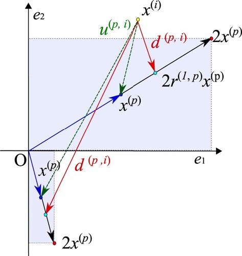
Now, we focus on the size of the search area of grey wolf i, $i\in W$ at iteration t. Since the size is mainly determined by ${\mathit{d}}^{(p,i)}\left(t\right)=|2{\mathit{r}}^{(p,1)}\otimes {\mathit{x}}^{\left(p\right)}(t)-{\mathit{x}}_j^{\left(i\right)}(t\left)\right|$, $p\in \{\alpha ,\text{β},\delta \}$, let us consider the upper bound ${\hat{d}}_j^{(p,i)}$ of jth component of ${\mathit{d}}^{(p,i)}\left(t\right)$ at iteration t, which is shown in Figure 1. Here, we define ${\mathit{u}}^{(p,i)}\left(t\right):={\mathit{x}}^{\left(p\right)}\left(t\right)-{\mathit{x}}^{\left(i\right)}\left(t\right)$. We can see that the jth component of $2{\mathit{r}}^{(p,1)}\otimes {\mathit{x}}^{\left(p\right)}$ is varied in $(0,2x_j^{\left(p\right)}(t\left)\right)$ or $\left(2x_j^{\left(p\right)}\right(t),0)$, $j\in N$, which are represented as light blue areas in Figure 1. Therefore, the upper bound ${\hat{d}}_j^{(p,i)}\left(t\right)$ is given by (7) $\begin{array}{rl}{\hat{d}}_j^{(p,i)}\left(t\right)& =max\left\{\right|x_j^{\left(i\right)}\left(t\right)|,|2x_j^{\left(p\right)}\left(t\right)-x_j^{\left(i\right)}\left(t\right)\left|\right\}\\ & =max\left\{\right|x_j^{\left(p\right)}\left(t\right)-u_j^{(p,i)}\left(t\right)|,\\ & +\left|x_j^{\left(p\right)}\right(t)+u_j^{(p,i)}(t\left)\right|\}\end{array}$(7) (8) $\begin{array}{rl}& =\{\begin{array}{ll}{x}_j^{\left(p\right)}\left(t\right)+\left|u_j^{(p,i)}\right(t\left)\right|& \text{if}{x}_j^{\left(p\right)}\left(t\right)\ge 0,\\ -x_j^{\left(p\right)}\left(t\right)+\left|u_j^{(p,i)}\right(t\left)\right|& \text{if}{x}_j^{\left(p\right)}\left(t\right)<0,\end{array}\\ & =\left|x_j^{\left(p\right)}\right(t\left)\right|+\left|u_j^{(p,i)}\right(t\left)\right|,j\in \{1,\dots ,n\}.\end{array}$(8) From the results we can see that $\Vert {\mathit{d}}^{(p,i)}\left(t\right)\Vert$ increases as $\Vert {\mathit{x}}^{\left(p\right)}\left(t\right)\Vert$ or $\Vert {\mathit{u}}^{\left(p\right)}\left(t\right)\Vert$ increases. It is reasonable to choose a large $\Vert {\mathit{d}}^{(p,i)}\left(t\right)\Vert$ for a large $\Vert {\mathit{u}}^{(p,i)}\left(t\right)\Vert$ because the solution ${\mathit{x}}^{\left(i\right)}\left(t\right)$ which is far from the three best solutions ${\mathit{x}}^{\left(p\right)}\left(t\right)$, $p\in \{\alpha ,\text{β},\delta \}$ should be changed drastically. However, it is not well-founded to choose a large $\Vert {\mathit{d}}^{(p,i)}\left(t\right)\Vert$ for a large $\Vert {\mathit{x}}^{\left(p\right)}\left(t\right)\Vert$ because $\Vert {\mathit{x}}^{\left(p\right)}\left(t\right)\Vert$ just represents the distance from the origin, which is simply a reference point in the coordinate representation, and thus, $\Vert {\mathit{x}}^{\left(p\right)}\left(t\right)\Vert$ does not contain any useful information for a search. This property can cause an inefficient search, which is discussed in Ref. [16].

From these results, we can see that when the problem has the global optimal solution at the origin, an intensive search around the origin, and an extensive search far from the origin can effectively work in the GWO. On the other hand, when the optimal solutions are far from the origin, the intensive and extensive searches cannot be expected to work so effectively. In the next subsection, we experimentally clarify the ineffective search of the GWO due to the property by using a large number of shifted problems in more detail than in work [16].

3.3. Numerical experiments

In this subsection, we investigate how search efficiency of GWO for (P2) changes as the shift vector $\mathit{s}$ is varied through numerical experiments, which analyzes the quantitative relevance such as the relationship between the size of the shift vector and the mean size of the search areas, the means of $\Vert {\mathit{d}}^{(\alpha ,i)}(t,l)\Vert$ and $\Vert \mathrm{\Delta }{\mathit{x}}^{(\alpha ,i)}(t,l)\Vert$, (9) $\begin{array}{rl}{d}_{\mathrm{m}}^{\left(\alpha \right)}\left(t\right)& =\sum _{l=1}^{50}\sum _{i\in W}\frac{\Vert {\mathit{d}}^{(\alpha ,i)}(t,l)\Vert }{50\left|W\right|},\\ \mathrm{\Delta }{x}_{\mathrm{m}}^{\left(\alpha \right)}\left(t\right)& =\sum _{l=1}^{50}\sum _{i\in W}\frac{\Vert \mathrm{\Delta }{\mathit{x}}^{(\alpha ,i)}(t,l)\Vert }{50\left|W\right|},\end{array}$(9) on 50 trials at iteration t, where ${\mathit{d}}^{(\alpha ,i)}(t,l)$ and $\mathrm{\Delta }{\mathit{x}}^{(\alpha ,i)}(t,l)$ denote vectors obtained at iteration t on trial l, respectively. In addition, we observed the mean of the best function values obtained on 50 trials at iteration t, (10) $\begin{array}{r}{f}_{\mathrm{m}}^{\left(\alpha \right)}\left(t\right)=\sum _{l=1}^{50}\frac{f_s\left({\mathit{x}}^{\left(\alpha \right)}\right(t,l\left)\right)}{50},\end{array}$(10) where ${\mathit{x}}^{\left(\alpha \right)}(t,l)$ denotes the best solution obtained at iteration t on trial l. The maximal number of iteration $t_{\max }$ is 5000, the number of wolves $\left|W\right|$ was 80, and we used $\mathit{a}\left(t\right)=2(1-t/t_{max})\mathbf{1}$ as mentioned at Section 2.

We used 18 basic functions of CEC'17 benchmark problems [22] (C1: BentCigar, C2: Sum of Different Power, C3: Zakharov, C4: Rosenbrock, C5: Rastrigin, C6: Expanded Schaffer F6, C7: Levy, C8: Modified Schwefel, C9: High Conditioned Elliptic, C10: Discus, C11: Ackley, C12: Weierstrass, C13: Griewank, C14: Katsuura, C15: HappyCat, C16: HGBat, C17: Expanded Griewank plus Rosenbrock, C18: Schaffer F7 ). In the experiments, relatively simple functions were used to compare the behavior of the original GWO for shift transformations. All functions have a hypercube constraint whose sides are 100, and functions C4, C15–C17 have the optimal solution at $\mathbf{1}$ or $-\mathbf{1}$ $\in {\mathrm{\Re }}^n$, while others have the zero-optimal solution. In addition, we used other two problems: O1:2n-minima Func. and O2:Schwefel Func., which have the optimal solution far from the origin as shown in Table 1. All problems have a hypercube constraint whose side is the same constant $c_s$, namely, $x_i^l=x_i^u=c_s$, $i\in N$. As a shift vector $\mathit{s}$, four vectors $\rho c_s\mathit{u}$, ρ ∈$\{0.0,0.1,0.5,0.9\}$ were used, where $\mathit{u}$ is a randomly selected unit vector, and thus, ρ determines the relative size of $\mathit{s}$ toward $c_s$. Note that (P2) with $\rho =0$ is equivalent to (P1).

Table 1. Benchmark problems.

Func.	Objective function and constraint	Optimal solution
$O1$: $2n$-minima	$\begin{array}{ll}min& \sum _{i=1}^n(x_i^4-16x_i^2+5x_i)-78.319n\\ \text{s.t.}& -5\le x_i\le 5,i\in N\end{array}$	$f\left({\mathit{x}}^{\ast }\right)=0$, ${\mathit{x}}^{\ast }=(-2.9,\dots ,-2.9{)}^{\mathrm{\top }}$
$O2$: Schwefel	$\begin{array}{ll}min& \sum _{i=1}^n-x_i\sin \left(\sqrt{\left|x_i\right|}\right)-418.98288727\times n\\ \text{s.t.}& -512\le x_i<512,i\in N\end{array}$	$f\left({\mathit{x}}^{\ast }\right)=0$, $\begin{array}{l}{\mathit{x}}^{\ast }=(420.968750,\dots ,\\ 420.968750{)}^{\mathrm{\top }}\end{array}$

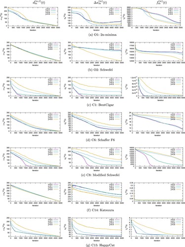
Figure 2 depicts the results of seven problems for which typical transitions of each of (9(9) $\begin{array}{rl}{d}_{\mathrm{m}}^{\left(\alpha \right)}\left(t\right)& =\sum _{l=1}^{50}\sum _{i\in W}\frac{\Vert {\mathit{d}}^{(\alpha ,i)}(t,l)\Vert }{50\left|W\right|},\\ \mathrm{\Delta }{x}_{\mathrm{m}}^{\left(\alpha \right)}\left(t\right)& =\sum _{l=1}^{50}\sum _{i\in W}\frac{\Vert \mathrm{\Delta }{\mathit{x}}^{(\alpha ,i)}(t,l)\Vert }{50\left|W\right|},\end{array}$(9) ) and (10(10) $\begin{array}{r}{f}_{\mathrm{m}}^{\left(\alpha \right)}\left(t\right)=\sum _{l=1}^{50}\frac{f_s\left({\mathit{x}}^{\left(\alpha \right)}\right(t,l\left)\right)}{50},\end{array}$(10) ) were observed. They are selected from all results obtained by the GWO to 20 benchmark problems with four shift vectors, respectively.

Figure 2. Means of $\Vert \mathrm{\Delta }{\mathit{x}}^{(\alpha ,i)}\left(t\right)\Vert$, $\Vert {\mathit{d}}^{(\alpha ,i)}\left(t\right)\Vert$, and $f\left({\mathit{x}}^{\left(\alpha \right)}\right(t\left)\right)$ for four shift vectors.

Furthermore, Table 2 indicates the mean function values and their standard deviations (SD) obtained by GWO for 20 benchmark problems with four shift vectors on 50 trials, where the first and second best values of the means or SDs obtained for the same problem with four shift vectors are indicated by bold and italic numbers, respectively.

Table 2. Comparison of results obtained by GWO for 20 benchmark problems (P1) and (P2) with three kinds of shift vectors ($\rho =0.1,0.5,0.9$).

	$\rho =0.0$		$\rho =0.1$		$\rho =0.5$		$\rho =0.9$
	Mean	SD	Mean	SD	Mean	SD	Mean	SD
O1	9.45E+02	1.55E+02	8.97E+02	1.56E+02	8.08E+02	1.07E+02	7.35E+02	1.25E+02
O2	1.47E+04	1.26E+03	1.44E+04	1.64E+03	1.41E+04	1.79E+03	1.22E+04	2.56E+03
C1	0.00E+00	0.00E+00	1.40E+08	5.83E+07	3.03E+09	1.19E+09	7.16E+09	2.48E+09
C2	0.00E+00	0.00E+00	1.39E+40	6.90E+40	1.52E+52	7.30E+52	1.13E+61	3.85E+61
C3	0.00E+00	0.00E+00	2.51E+02	9.33E+01	5.97E+03	1.72E+03	1.47E+04	5.48E+03
C4	4.55E+01	7.82E−01	5.46E+01	2.76E+00	2.63E+02	8.43E+01	5.81E+02	2.56E+02
C5	0.00E+00	0.00E+00	5.62E+01	1.27E+01	1.30E+02	2.12E+01	1.99E+02	2.50E+01
C6	1.33E+01	4.10E+00	1.32E+01	4.49E+00	1.81E+01	1.90E+00	2.00E+01	1.06E+00
C7	2.15E+00	2.66E−01	5.78E+01	1.74E+01	8.24E+02	1.90E+02	3.27E+03	2.20E+03
C8	1.82E−11	0.00E+00	1.10E+03	3.90E+02	5.01E+03	1.51E+03	5.02E+03	1.12E+03
C9	0.00E+00	0.00E+00	1.93E+06	1.19E+06	3.64E+07	1.76E+07	9.40E+07	5.14E+07
C10	0.00E+00	0.00E+00	6.77E+02	1.66E+02	1.33E+04	2.76E+03	3.32E+04	1.02E+04
C11	2.05E+01	5.54E−02	2.05E+01	5.44E−02	2.05E+01	5.03E−02	2.05E+01	6.35E−02
C12	0.00E+00	0.00E+00	6.28E+00	1.25E+00	1.68E+01	3.15E+00	2.37E+01	3.60E+00
C13	0.00E+00	0.00E+00	2.31E+00	5.82E−01	2.80E+01	1.11E+01	6.76E+01	3.11E+01
C14	2.18E−02	5.15E−03	2.05E−02	4.53E−03	2.38E−02	4.60E−03	2.45E−02	6.12E−03
C15	5.80E−01	6.45E−02	5.60E−01	7.21E−02	5.41E−01	7.21E−02	7.02E−01	1.96E−01
C16	4.11E−01	6.45E−02	3.76E−01	7.86E−02	1.67E+00	3.87E+00	1.66E+01	1.09E+01
C17	1.85E+01	2.51E+00	1.47E+01	5.19E+00	2.57E+02	2.13E+02	8.56E+03	1.41E+04
C18	5.09E−01	1.25E+00	9.24E−01	1.15E+00	2.43E+00	3.42E+00	2.77E+00	4.83E+00

First, we focus on the results of problems C1–C18 which have the optimal solution at the origin or close to the origin. From the figure and table, we can see in most of problems with a small ρ, the GWO can find exactly the global optimal solutions or considerably high-quality solutions, and that $\Vert \mathrm{\Delta }{\mathit{x}}^{(\alpha ,i)}\left(t\right)\Vert$ and $\Vert {\mathit{d}}^{(\alpha ,i)}\left(t\right)\Vert$ are large at early stages of the search, gradually decrease and finally approach zero, which shows that the adjustment of the size of search area is appropriate. On the other hand, GWO finds considerably low-quality solutions for the problems with a large ρ. In this case, although $\Vert \mathrm{\Delta }{\mathit{x}}^{(\alpha ,i)}\left(t\right)\Vert$ and $\Vert {\mathit{d}}^{(\alpha ,i)}\left(t\right)\Vert$ are decreasing, the rate of decrease becomes slower as ρ becomes larger. In particular, $\Vert {\mathit{d}}^{(\alpha ,i)}\left(t\right)\Vert$ is relatively large until the final stage, which means that the search is not sufficiently intensified. Moreover, the function value does not decrease as smoothly as the problem with smaller ρ, and the function values obtained finally are considerably worse for the problem with a larger ρ. These results show that adjustment of the search area is not appropriate, which are consistent with the previous discussion.

Next, let us consider the two problems, O1 and O2, in which the optimal solution is far from the origin. In these cases, the mean of obtained function values is smallest for (P2) with $\sigma =0.9$, and the obtained solutions are not overwhelmingly high quality, which are considerably different from the case for problems having the zero-optimal solution. In these cases, we find that the search of GWO is not so efficient regardless of the shift transformations.

From the above observations, the following conclusions can be derived. Since, in general, many global optimization problems can be expected to have many local solutions other than the origin, the technique of adjusting the search area in GWO as mentioned above can be regarded as a fatal drawback as a metaheuristic method, and it is difficult to find high-quality solutions by the GWO to many real-world problems. Therefore, in the subsequent sections, we propose modified GWOs to overcome the drawbacks which were pointed out in this section.

4. Shift-invariant GWO

4.1. Modification of GWO-R

In this subsection, we first introduce the GWO-R, which was proposed in Ref. [16], and show that it is shift-invariant to overcome the drawback of the original GWO. Secondly, we theoretically and experimentally point out that the intensification of the GWO-R is insufficient in the final stages and propose its modified method such that its search areas are more reasonably controlled than GWO-R. Then, we show theoretically the shift-invariance of the GWO-R and the modified GWO-R.

In GWO-R, the point $\mathit{\mu }\left(t\right)$ called a reference point is used to adjust adaptively the search area of each grey wolf i $\in W$ on the basis of the distance of $\mathit{\mu }\left(t\right)$ to ${\mathit{x}}^{\left(p\right)}\left(t\right)$, $p\in \{\alpha ,\text{β},\delta \}$ or ${\mathit{x}}^{\left(i\right)}\left(t\right)$: (11) $\begin{array}{rl}& {\mathit{d}}^{(p,i)}\left(t\right):=\left|2c_{m}b\right(t){\mathit{r}}^{(p,1)}\\ & \otimes ({\mathit{x}}^{\left(p\right)}-\mathit{\mu }(t\left)\right)-\left({\mathit{x}}^{\left(i\right)}\right(t)-\mathit{\mu }(t\left)\right)|,\end{array}$(11) (12) $\begin{array}{rl}& {\mathit{\xi }}^{(p,i)}\left(t\right):={\mathit{x}}^{\left(i\right)}\left(t\right)+2b\left(t\right)(2{\mathit{r}}^{(p,2)}-1)\otimes {\mathit{d}}^{(p.i)}\left(t\right),\\ & p\in \{\alpha ,\text{β},\delta \}\end{array}$(12) (13) $\begin{array}{rl}& {\mathit{x}}^{\left(i\right)}(t+1):=\frac{1}{3}\sum _{p\in \{\alpha ,\text{β},\delta \}}{\mathit{\xi }}^{(p,i)}\left(t\right),\end{array}$(13) where (11(11) $\begin{array}{rl}& {\mathit{d}}^{(p,i)}\left(t\right):=\left|2c_{m}b\right(t){\mathit{r}}^{(p,1)}\\ & \otimes ({\mathit{x}}^{\left(p\right)}-\mathit{\mu }(t\left)\right)-\left({\mathit{x}}^{\left(i\right)}\right(t)-\mathit{\mu }(t\left)\right)|,\end{array}$(11) ) was derived by replacing $2{\mathit{r}}^{(p,1)}$ with $c_{m}b\left(t\right){\mathit{r}}^{(p,1)}$ in (1(1) $\begin{array}{rl}& {\mathit{d}}^{(p,i)}\left(t\right):=|2{\mathit{r}}^{(p,1)}\otimes {\mathit{x}}^{\left(p\right)}(t)-{\mathit{x}}^{\left(i\right)}(t\left)\right|,\end{array}$(1) ), $b\left(t\right)$ is given by $b\left(t\right)=1-t/t_{max}$, and $c_m$ is a positive value for adjusting the search area. The GWO using (11(11) $\begin{array}{rl}& {\mathit{d}}^{(p,i)}\left(t\right):=\left|2c_{m}b\right(t){\mathit{r}}^{(p,1)}\\ & \otimes ({\mathit{x}}^{\left(p\right)}-\mathit{\mu }(t\left)\right)-\left({\mathit{x}}^{\left(i\right)}\right(t)-\mathit{\mu }(t\left)\right)|,\end{array}$(11) )–(13(13) $\begin{array}{rl}& {\mathit{x}}^{\left(i\right)}(t+1):=\frac{1}{3}\sum _{p\in \{\alpha ,\text{β},\delta \}}{\mathit{\xi }}^{(p,i)}\left(t\right),\end{array}$(13) ) is called GWO with reference points (GWO-R).

The reference point $\mathit{\mu }\left(t\right)$ was selected by using information obtained until iteration t through the search process. As the reference point, three candidates were proposed as follows:

1. Centroid of all pbests:${\mathit{\mu }}^{\left(1\right)}\left(t\right)=\frac{1}{\left|W\right|}\sum _{i\in W}{\mathit{p}}^{\left(i\right)}\left(t\right)$,

2. Centroid of all grey wolves:${\mathit{\mu }}^{\left(2\right)}\left(t\right)=\frac{1}{\left|W\right|}\sum _{i\in W}{\mathit{x}}^{\left(i\right)}\left(t\right)$,

3. Centroid of three best solutions:${\mathit{\mu }}^{\left(3\right)}\left(t\right)=\frac{1}{3}\left({\mathit{x}}^{\left(\alpha \right)}\right(t)+{\mathit{x}}^{\left(\text{β}\right)}(t)+{\mathit{x}}^{\left(\delta \right)}(t\left)\right)$,

where ${\mathit{p}}^{\left(i\right)}\left(t\right)$, $i\in W$ denotes the personal bests (pbests), which is the best solution found by grey wolf i until iteration t as follows: $\begin{array}{r}{\mathit{p}}^{\left(i\right)}\left(t\right)=\mathrm{argmin}\left\{f\right(\mathit{x}\left)|\mathit{x}\in \{{\mathit{x}}^{\left(i\right)}\left(\tau \right){\}}_{\tau \in \{1,\dots ,t\}}\right\}.\end{array}$The pbests have been used in PSO, which exploits information obtained by each search agent. In addition, as reference points, authors introduced internally dividing point of two reference points, ${\mathit{\mu }}^{\left(i\right)}\left(t\right)$ and ${\mathit{\mu }}^{\left(j\right)}\left(t\right)$, selected from the three kinds of candidates, in which its weights vary linearly as follows: $\begin{array}{rl}{\mathit{\mu }}^{(i,j)}& =\frac{1}{t_{max}}\left((t_{max}-t){\mathit{\mu }}^{\left(i\right)}\right(t)+t{\mathit{\mu }}^{\left(j\right)}(t\left)\right),\\ & i\ne j\in \{1,2,3\}.\end{array}$By using these kinds of reference points, updating systems (11(11) $\begin{array}{rl}& {\mathit{d}}^{(p,i)}\left(t\right):=\left|2c_{m}b\right(t){\mathit{r}}^{(p,1)}\\ & \otimes ({\mathit{x}}^{\left(p\right)}-\mathit{\mu }(t\left)\right)-\left({\mathit{x}}^{\left(i\right)}\right(t)-\mathit{\mu }(t\left)\right)|,\end{array}$(11) )–(13(13) $\begin{array}{rl}& {\mathit{x}}^{\left(i\right)}(t+1):=\frac{1}{3}\sum _{p\in \{\alpha ,\text{β},\delta \}}{\mathit{\xi }}^{(p,i)}\left(t\right),\end{array}$(13) ) of the GWO-R are shift-invariant, as shown at the end of this subsection,

Moreover, in Ref. [16], the relations between the upper bound of ${\mathit{d}}^{(p,i)}\left(t\right)$ and the difference vector between the best solution and the reference point, namely ${\mathit{v}}^{\left(p\right)}:={\mathit{x}}^{\left(p\right)}\left(t\right)-\mathit{\mu }\left(t\right)$, were derived in the similar way in 3.2 as follows: (14) $\begin{array}{rl}{\hat{d}}_j^{(p,i)}\left(t\right)& =max\{\left|v_j^{\left(p\right)}\right(t)-u_j^{(p,i)}(t\left)\right|,\\ & \left|\right(2c_{m}b\left(t\right)-1\left)v_j^{\left(p\right)}\right(t)+u_j^{(p,i)}(t\left)\right|\},\end{array}$(14) The relations indicate that the search process can be classified into three stages: in the first stage the upper bound ${\hat{d}}_j^{(p,i)}\left(t\right)$ increases with a large proportional constant to $\left|v_j^{\left(p\right)}\right|$, which can be considered to be an extensive search, and in the second and third stages, it increases with a small proportional constant, which means an intensive search. These results show that independently of the distance between the optimal solution and the origin, GWO-R gradually shifts from diverse to intensive search as the search progresses. At the same time, the effective search by GWO-R was reported through numerical experiments in Ref. [16].

Furthermore, we can observe that in the first and second stages, under the assumption that ${\mathit{u}}^{(p,i)}\left(t\right)={\mathit{x}}^{\left(p\right)}\left(t\right)-{\mathit{x}}^{\left(i\right)}\left(t\right)$ is fixed, ${\hat{d}}_j^{(p,i)}\left(t\right)$ is minimal when $x_j^{\left(p\right)}\left(t\right)={\mu }_j\left(t\right)$. The observation means that the search area is minimal when the best solution is equal to the reference point. Such behavior is reasonable because if additionally ${\mathit{u}}^{\left(p\right)}\left(t\right)=\mathbf{0}$ holds, namely, ${\mathit{x}}^{\left(i\right)}\left(t\right)={\mathit{x}}^{\left(p\right)}\left(t\right)=\mathit{\mu }\left(t\right)$, the size of the search area is zero.

On the other hand, under the same assumption, only in the third stage, ${\hat{d}}_j^{(p,i)}\left(t\right)$ is not minimal even if $x_j^{\left(p\right)}\left(t\right)={\mu }_j\left(t\right)$, which is not reasonable. In such cases, the detailed search may be insufficient.

Therefore, in this paper, we modify the updating system (11(11) $\begin{array}{rl}& {\mathit{d}}^{(p,i)}\left(t\right):=\left|2c_{m}b\right(t){\mathit{r}}^{(p,1)}\\ & \otimes ({\mathit{x}}^{\left(p\right)}-\mathit{\mu }(t\left)\right)-\left({\mathit{x}}^{\left(i\right)}\right(t)-\mathit{\mu }(t\left)\right)|,\end{array}$(11) ) such that ${\hat{d}}_j^{(p,i)}\left(t\right)$ is minimal when ${\mathit{x}}^{\left(p\right)}\left(t\right)=\mathit{\mu }\left(t\right)$ as follows: (15) $\begin{array}{rl}{\mathit{d}}^{(p,i)}\left(t\right)& :=|\left(c_{m}b\right(t){\mathit{r}}^{(p,1)}+1)\\ & \otimes \left({\mathit{x}}^{\left(p\right)}\right(t)-\mathit{\mu }(t\left)\right)-\left({\mathit{x}}^{\left(i\right)}\right(t)-\mathit{\mu }(t\left)\right)|.\end{array}$(15) The GWO with updating systems (12(12) $\begin{array}{rl}& {\mathit{\xi }}^{(p,i)}\left(t\right):={\mathit{x}}^{\left(i\right)}\left(t\right)+2b\left(t\right)(2{\mathit{r}}^{(p,2)}-1)\otimes {\mathit{d}}^{(p.i)}\left(t\right),\\ & p\in \{\alpha ,\text{β},\delta \}\end{array}$(12) ), (13(13) $\begin{array}{rl}& {\mathit{x}}^{\left(i\right)}(t+1):=\frac{1}{3}\sum _{p\in \{\alpha ,\text{β},\delta \}}{\mathit{\xi }}^{(p,i)}\left(t\right),\end{array}$(13) ) and (15(15) $\begin{array}{rl}{\mathit{d}}^{(p,i)}\left(t\right)& :=|\left(c_{m}b\right(t){\mathit{r}}^{(p,1)}+1)\\ & \otimes \left({\mathit{x}}^{\left(p\right)}\right(t)-\mathit{\mu }(t\left)\right)-\left({\mathit{x}}^{\left(i\right)}\right(t)-\mathit{\mu }(t\left)\right)|.\end{array}$(15) ) is called simplified GWO-R (GWO-SR), in which the search process can be classified into two stages, and under the same assumptions as above, the upper bound ${\hat{d}}_j^{(p,i)}\left(t\right)$ is minimal in all stages when ${\mathit{x}}^{\left(i\right)}\left(t\right)$, ${\mathit{x}}^{\left(p\right)}\left(t\right)$ and $\mathit{\mu }\left(t\right)$ are equal. The properties can be shown as follows.

Now, we analyze the search area of each grey wolf. First, let us consider the upper bound ${\hat{d}}_j^{(p,i)}\left(t\right)$ of ${\mathit{d}}^{\left(i\right)}\left(t\right)$ in (15(15) $\begin{array}{rl}{\mathit{d}}^{(p,i)}\left(t\right)& :=|\left(c_{m}b\right(t){\mathit{r}}^{(p,1)}+1)\\ & \otimes \left({\mathit{x}}^{\left(p\right)}\right(t)-\mathit{\mu }(t\left)\right)-\left({\mathit{x}}^{\left(i\right)}\right(t)-\mathit{\mu }(t\left)\right)|.\end{array}$(15) ). In the same way to derivate (14(14) $\begin{array}{rl}{\hat{d}}_j^{(p,i)}\left(t\right)& =max\{\left|v_j^{\left(p\right)}\right(t)-u_j^{(p,i)}(t\left)\right|,\\ & \left|\right(2c_{m}b\left(t\right)-1\left)v_j^{\left(p\right)}\right(t)+u_j^{(p,i)}(t\left)\right|\},\end{array}$(14) ), we have that (16) $\begin{array}{rl}{\hat{d}}_j^{(p,i)}\left(t\right)& =max\{\left|x_j^{\left(i\right)}\right(t)-{\mu }_j(t\left)\right|,\\ & \times \left|\right(c_{m}b\left(t\right)+1)\left(x_j^{\left(p\right)}\right(t)-{\mu }_j(t\left)\right)\\ & -\left(x_j^{\left(i\right)}\right(t)-{\mu }_j(t\left)\right)|\}\\ & =max\{\left|v_j^{\left(p\right)}\right(t)-u_j^{(p,i)}(t\left)\right|,\\ & \times \left|c_{m}b\right(t\left)v_j^{\left(p\right)}\right(t)+u_j^{(p,i)}(t\left)\right|\}.\end{array}$(16) Thus, ${\hat{d}}_j^{(p,i)}\left(t\right)$ can be evaluated by dividing into the following cases: (17) $\begin{array}{rl}& \text{If}{c}_{m}b\left(t\right)=1,\text{then}{\hat{d}}_j^{(p,i)}\left(t\right)=\left|v_j^{\left(p\right)}\right(t\left)\right|+\left|u_j^{(p,i)}\right(t\left)\right|,\end{array}$(17) (18) $\begin{array}{rl}& \text{If}{\delta }_j^{(p,i)}\left(t\right)v_j^{\left(p\right)}\left(t\right)\in [\frac{2\left|u_j^{(p,i)}\right|}{1-c_{m}b\left(t\right)},0],c_{m}b\left(t\right)>1,\\ & \text{or}{\delta }_j^{(p,i)}\left(t\right)v_j^{\left(p\right)}\left(t\right)\notin [0,\frac{2\left|u_j^{(p,i)}\right|}{1-c_{m}b\left(t\right)}],c_{m}b\left(t\right)<1,\\ & \text{then}{\hat{d}}_j^{(p,i)}\left(t\right)=\left|v_j^{\left(p\right)}\right(t)-u_j^{(p,i)}(t\left)\right|\\ & \le \left|v_j^{\left(p\right)}\right(t\left)\right|+\left|u_j^{(p,i)}\right(t\left)\right|,\end{array}$(18) (19) $\begin{array}{rl}& \text{If}{\delta }_j^{(p,i)}\left(t\right)v_j^{\left(p\right)}\left(t\right)\notin [\frac{2\left|u_j^{(p,i)}\right|}{1-c_{m}b\left(t\right)},0],c_{m}b\left(t\right)>1,\\ & \text{or}{\delta }_j^{(p,i)}\left(t\right)v_j^{\left(p\right)}\left(t\right)\in [0,\frac{2\left|u_j^{(p,i)}\right|}{1-c_{m}b\left(t\right)}],c_{m}b\left(t\right)<1,\\ & \text{then}{\hat{d}}_j^{(p,i)}\left(t\right)=\left|c_{m}b\right(t\left)v_j^{\left(p\right)}\right(t)+u_j^{(p,i)}|\\ & \le \left|c_{m}b\right(t\left)v_j^{\left(p\right)}\right(t\left)\right|+\left|u_j^{(p,i)}\right|,\end{array}$(19) where we define ${\delta }_j^{(p,i)}\left(t\right):=u_j^{(p,i)}\left(t\right)/\left|u_j^{(p,i)}\right(t\left)\right|$.

Note that $c_{m}b\left(t\right)<1$ and $c_{m}b\left(t\right)>1$ mean the first and second halves of the search such that $t<t_s$ and $t>t_s$, respectively, and $t_s:=(1-\frac{1}{c_m})t_{max}$ is the iteration at which the two kinds of searches are switched, as mentioned below:

From (17(17) $\begin{array}{rl}& \text{If}{c}_{m}b\left(t\right)=1,\text{then}{\hat{d}}_j^{(p,i)}\left(t\right)=\left|v_j^{\left(p\right)}\right(t\left)\right|+\left|u_j^{(p,i)}\right(t\left)\right|,\end{array}$(17) ), (18(18) $\begin{array}{rl}& \text{If}{\delta }_j^{(p,i)}\left(t\right)v_j^{\left(p\right)}\left(t\right)\in [\frac{2\left|u_j^{(p,i)}\right|}{1-c_{m}b\left(t\right)},0],c_{m}b\left(t\right)>1,\\ & \text{or}{\delta }_j^{(p,i)}\left(t\right)v_j^{\left(p\right)}\left(t\right)\notin [0,\frac{2\left|u_j^{(p,i)}\right|}{1-c_{m}b\left(t\right)}],c_{m}b\left(t\right)<1,\\ & \text{then}{\hat{d}}_j^{(p,i)}\left(t\right)=\left|v_j^{\left(p\right)}\right(t)-u_j^{(p,i)}(t\left)\right|\\ & \le \left|v_j^{\left(p\right)}\right(t\left)\right|+\left|u_j^{(p,i)}\right(t\left)\right|,\end{array}$(18) ) and (19(19) $\begin{array}{rl}& \text{If}{\delta }_j^{(p,i)}\left(t\right)v_j^{\left(p\right)}\left(t\right)\notin [\frac{2\left|u_j^{(p,i)}\right|}{1-c_{m}b\left(t\right)},0],c_{m}b\left(t\right)>1,\\ & \text{or}{\delta }_j^{(p,i)}\left(t\right)v_j^{\left(p\right)}\left(t\right)\in [0,\frac{2\left|u_j^{(p,i)}\right|}{1-c_{m}b\left(t\right)}],c_{m}b\left(t\right)<1,\\ & \text{then}{\hat{d}}_j^{(p,i)}\left(t\right)=\left|c_{m}b\right(t\left)v_j^{\left(p\right)}\right(t)+u_j^{(p,i)}|\\ & \le \left|c_{m}b\right(t\left)v_j^{\left(p\right)}\right(t\left)\right|+\left|u_j^{(p,i)}\right|,\end{array}$(19) ), we can see that in the first half, ${\hat{d}}_j^{(p,i)}\left(t\right)$ increases with proportional constant $c_{m}b\left(t\right)$ $(>1)$ for large $\left|v_j^{\left(p\right)}\right(t\left)\right|$, and does with 1 for small $\left|v_j^{\left(p\right)}\right(t\left)\right|$, respectively, which widens the search area at a relatively high rate according to $\Vert {\mathit{v}}^{\left(p\right)}\left(t\right)\Vert$, and that in the second half of the search, ${\hat{d}}_j^{(p,i)}\left(t\right)$ increases with the proportional constant 1 for large $\left|v_j^{\left(p\right)}\right(t\left)\right|$, and does with $c_{m}b\left(t\right)(<1)$ for small $\left|v_j^{\left(p\right)}\right(t\left)\right|$, respectively, which means that the effect of $\Vert {\mathit{v}}^{\left(p\right)}\left(t\right)\Vert$ 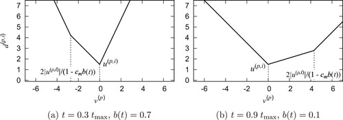on the search area is relatively small. These relations are depicted in Figure 3, in which $c_m$ was chosen to be 3.0, and the switching occurs at $t_s=(1-\frac{1}{c_m})t_{max}=\frac{2}{3}{t}_{max}$. The same $c_m$ was used in the numerical experiment at the next subsection. The results coincide with the above results. Furthermore, note that the results show that the upper bound ${\hat{d}}_j^{(p,i)}\left(t\right)$ is always minimal at $x_j^{\left(p\right)}\left(t\right)={\mu }_j\left(t\right)$ under the assumption that ${\mathit{u}}^{(p,i)}\left(t\right)$ is fixed, which means that the intensive search of GWO-SR is more reasonable than that of GWO-R.

Figure 3. Relation between ${\hat{d}}^{(p,i)}\left(t\right)$ and $v^{\left(p\right)}\left(t\right)$ when $c_m=3$ and $u^{(p,i)}=1.5$.

As discussed above, the search of the GWO-SR aims to suitably adjust the search area in a feasible way for more general cases. Note that $c_m$ determines not only the proportional constant $c_{m}b\left(t\right)$ of the search but also the switching iteration $t_s$. Thus, an appropriate selection of $c_m$ can tune the balance between diversification and intensification of the search.

Finally, we theoretically show the invariance of GWO-R and GWO-SR. Since in the updating systems (11(11) $\begin{array}{rl}& {\mathit{d}}^{(p,i)}\left(t\right):=\left|2c_{m}b\right(t){\mathit{r}}^{(p,1)}\\ & \otimes ({\mathit{x}}^{\left(p\right)}-\mathit{\mu }(t\left)\right)-\left({\mathit{x}}^{\left(i\right)}\right(t)-\mathit{\mu }(t\left)\right)|,\end{array}$(11) ), (12(12) $\begin{array}{rl}& {\mathit{\xi }}^{(p,i)}\left(t\right):={\mathit{x}}^{\left(i\right)}\left(t\right)+2b\left(t\right)(2{\mathit{r}}^{(p,2)}-1)\otimes {\mathit{d}}^{(p.i)}\left(t\right),\\ & p\in \{\alpha ,\text{β},\delta \}\end{array}$(12) ), (13(13) $\begin{array}{rl}& {\mathit{x}}^{\left(i\right)}(t+1):=\frac{1}{3}\sum _{p\in \{\alpha ,\text{β},\delta \}}{\mathit{\xi }}^{(p,i)}\left(t\right),\end{array}$(13) ) of GWO-R, or in (12(12) $\begin{array}{rl}& {\mathit{\xi }}^{(p,i)}\left(t\right):={\mathit{x}}^{\left(i\right)}\left(t\right)+2b\left(t\right)(2{\mathit{r}}^{(p,2)}-1)\otimes {\mathit{d}}^{(p.i)}\left(t\right),\\ & p\in \{\alpha ,\text{β},\delta \}\end{array}$(12) ), (13(13) $\begin{array}{rl}& {\mathit{x}}^{\left(i\right)}(t+1):=\frac{1}{3}\sum _{p\in \{\alpha ,\text{β},\delta \}}{\mathit{\xi }}^{(p,i)}\left(t\right),\end{array}$(13) ), (15(15) $\begin{array}{rl}{\mathit{d}}^{(p,i)}\left(t\right)& :=|\left(c_{m}b\right(t){\mathit{r}}^{(p,1)}+1)\\ & \otimes \left({\mathit{x}}^{\left(p\right)}\right(t)-\mathit{\mu }(t\left)\right)-\left({\mathit{x}}^{\left(i\right)}\right(t)-\mathit{\mu }(t\left)\right)|.\end{array}$(15) ) of GWO-SR, the position of grey wolf i is updated by using only difference vectors between $\mathit{\mu }\left(t\right)$ and ${\mathit{x}}^{\left(i\right)}$ or ${\mathit{x}}^{\left(p\right)}$, we can show shift-invariance of them as follows:

Theorem 4.1

GWO-R and GWO-SR are shift-invariant in the coordinate representation of the optimization problem.

Proof.

In the same way to Theorem 3.2, we assume that ${\mathit{x}}^{\left(i\right)}$, ${\overline{\mathit{x}}}^{\left(i\right)}$, ${\mathit{x}}^{\left(p\right)}$ and ${\overline{\mathit{x}}}^{\left(p\right)}$, $p\in \{\alpha ,\text{β},\delta \}$ satisfy (4(4) $\begin{array}{r}{\overline{\mathit{x}}}^{\left(i\right)}={\mathit{x}}^{\left(i\right)}+\mathit{s},i\in I,\end{array}$(4) ). In addition, $\mathit{\mu }\left(t\right)$ and $\overline{\mathit{\mu }}\left(t\right)$ denote the reference points in the original and shifted coordinate systems, namely for (P1) and (P2), respectively. Then, since from the definition of the reference point, $\mathit{\mu }\left(t\right)$ is a weighted sum of points satisfying the relation (4(4) $\begin{array}{r}{\overline{\mathit{x}}}^{\left(i\right)}={\mathit{x}}^{\left(i\right)}+\mathit{s},i\in I,\end{array}$(4) ), we have that $\overline{\mathit{\mu }}\left(t\right)=\mathit{\mu }\left(t\right)+\mathit{s}$, which means that ${\mathit{x}}^{\left(p\right)}\left(t\right)-\mathit{\mu }\left(t\right)={\overline{\mathit{x}}}^{\left(p\right)}\left(t\right)-\overline{\mathit{\mu }}\left(t\right)$, p $\in \{\alpha ,\text{β},\delta \}$, and ${\mathit{x}}^{\left(i\right)}\left(t\right)-\mathit{\mu }\left(t\right)={\overline{\mathit{x}}}^{\left(i\right)}\left(t\right)-\overline{\mathit{\mu }}\left(t\right)$, $i\in W$. Therefore, the relation ${\mathit{d}}^{(p,i)}\left(t\right)={\overline{\mathit{d}}}^{(p,i)}\left(t\right)$ always holds at t + 1 if all random variables are the same in both systems. As a results, the position of any grey wolf satisfies the relation (5(5) $\begin{array}{r}{\overline{\mathit{x}}}_{\mathrm{new}}^{\left(i\right)}={\mathit{x}}_{\mathrm{new}}^{\left(i\right)}+\mathit{s},i\in I,\end{array}$(5) ).

4.2. Numerical experiments

In this subsection, we applied GWO-R and GWO-SR to the same problems (P) with no shift-transformation as 3.3, namely, twenty 50-dimensional problems. Note that even if they are applied to (P2) with different shift vectors, the same results are obtained because of shift-invariance of them. We compared GWO-SRs with different reference points and GWO-R with ${\mathit{\mu }}^{(1,2)}$. In Ref. [16], GWO-R with ${\mathit{\mu }}^{(1,2)}$ was shown to have better performance than others. We compared the mean function values of the best solutions obtained by GWO-R and GWO-SR on 50 trials. The maximal number of iteration $t_{\max }$ was 5000, the number of wolves $\left|W\right|$ was 80, the constant $c_m$ of GWO-R was 1.5, and $c_m$ of GWO-SR was 3, which was selected in the preliminary experiments.

Table 3. Comparison of results obtained by GWO-SRs with seven different reference points and GWO-R with ${\mathit{\mu }}^{(1,2)}$ for 20 benchmark problems (P1).

Prob.	GWO-SR							GWO-R
No.	${\mathit{\mu }}^{\left(1\right)}$	${\mathit{\mu }}^{\left(2\right)}$	${\mathit{\mu }}^{\left(3\right)}$	${\mathit{\mu }}^{(1,2)}$	${\mathit{\mu }}^{(2,1)}$	${\mathit{\mu }}^{(1,3)}$	${\mathit{\mu }}^{(3,1)}$	${\mathit{\mu }}^{(1,2)}$
O1	3.99E+02	4.25E+02	4.33E+02	3.86E+02	4.14E+02	3.94E+02	4.52E+02	4.24E+02
O2	6.54E+03	6.82E+03	6.80E+03	6.49E+03	6.56E+03	6.47E+03	6.31E+03	6.08E+03
C1	1.79E−11	2.78E−09	1.60E+09	1.52E−14	4.19E−14	4.56E−12	1.24E−06	7.41E−09
C2	2.35E+50	1.45E+62	2.04E+72	1.46E+43	2.53E+60	1.36E+37	1.41E+72	1.94E+46
C3	4.34E−08	9.39E+02	9.27E+03	4.00E−06	1.18E+02	3.56E−06	8.95E+02	1.61E−03
C4	5.19E+01	7.21E+01	4.05E+02	5.40E+01	7.48E+01	5.31E+01	8.01E+01	5.67E+01
C5	7.84E+01	1.94E+02	2.16E+02	7.51E+01	1.83E+02	8.02E+01	2.07E+02	1.19E+02
C6	1.72E+01	1.76E+01	1.85E+01	1.77E+01	1.73E+01	1.76E+01	1.88E+01	1.80E+01
C9	1.53E+03	8.77E+03	9.70E+03	1.98E+03	8.19E+03	1.96E+03	8.00E+03	3.00E+03
C10	2.82E+03	5.40E+03	6.13E+03	2.77E+03	4.97E+03	2.98E+03	5.80E+03	3.53E+03
C11	4.50E−15	4.70E−09	3.99E+07	9.60E−18	4.04E−13	2.31E−15	2.04E−04	1.16E−10
C12	7.26E−16	8.01E−16	1.38E+04	5.06E−20	1.44E−19	1.57E−18	1.48E−08	2.87E−14
C13	2.06E+01	2.01E+01	2.00E+01	2.06E+01	2.05E+01	2.06E+01	2.02E+01	2.09E+01
C14	7.84E−01	3.91E+00	7.39E+00	8.72E−01	3.39E+00	1.06E+00	6.56E+00	4.72E+00
C15	2.81E−02	3.69E−02	2.00E+01	1.95E−02	5.58E−02	1.17E−02	1.13E−01	3.29E−02
C16	4.70E−02	2.27E−17	0.00E+00	4.80E−02	1.02E−03	4.69E−02	1.08E−17	9.05E−02
C17	4.48E−01	5.40E−01	6.01E−01	4.89E−01	5.30E−01	4.51E−01	5.91E−01	4.93E−01
C18	6.12E−01	6.04E−01	5.10E+00	6.33E−01	6.33E−01	5.54E−01	6.25E−01	5.18E−01
C19	1.41E+01	6.36E+01	1.12E+04	1.92E+01	3.03E+01	2.35E+01	4.85E+01	1.84E+01
C20	4.67E−02	1.14E−01	3.06E−01	4.48E−02	5.24E−02	6.21E−02	1.24E−01	4.85E−02

Table 3 shows the result obtained by GWO-R using ${\mathit{\mu }}^{(1,2)}$ and GWO-SRs using ${\mathit{\mu }}^{\left(i\right)}$, i = 1, 2, 3 and four internally dividing points, ${\mathit{\mu }}^{(1,2)}$, ${\mathit{\mu }}^{(2,1)}$, ${\mathit{\mu }}^{(1,3)}$ and ${\mathit{\mu }}^{(3,1)}$, which are the first to fourth best results in ones obtained by GWO-SRs using internally dividing points of all combinations of two points, ${\mathit{\mu }}^{(i,j)}$, $i\ne j$ ∈$\{1,2,3\}$. We can see that GWO-SRs with ${\mathit{\mu }}^{\left(1\right)}$, ${\mathit{\mu }}^{(1,2)}$ and ${\mathit{\mu }}^{(1,3)}$ obtained better solutions than others, which demonstrates that it is advantageous to use the centroid of pbests for the diversification in the first half of the search, and the centroid of ${\mathit{x}}^{\left(i\right)}$, $i\in W$ or ${\mathit{x}}^{\left(p\right)}$, $i\in \{\alpha ,\text{β},\delta \}$ for the intensification in its second half. At the same time, the results indicate that the selection of the reference point is considerably important because the reference point is a significant criterion to adjust the size of the search area.

Next, comparing GWO-R with GWO-SR using the same ${\mathit{\mu }}^{(1,2)}$, we can observe that GWO-SR is superior to GWO-R, which indicates that the method of adjusting reasonably the search area works effectively in GWO-SR due to (15(15) $\begin{array}{rl}{\mathit{d}}^{(p,i)}\left(t\right)& :=|\left(c_{m}b\right(t){\mathit{r}}^{(p,1)}+1)\\ & \otimes \left({\mathit{x}}^{\left(p\right)}\right(t)-\mathit{\mu }(t\left)\right)-\left({\mathit{x}}^{\left(i\right)}\right(t)-\mathit{\mu }(t\left)\right)|.\end{array}$(15) ). In addition, since most of the results of the GWO-SR are better than those of the original GWO for (P2) with different shift vectors ($\rho \ne 0$) shown in Table 2, we can conclude that the proposed GWO-SR is more useful than the original GWO. These results and the reasonable control of the search areas in GWO-SR show that if the reference point is a temporal prey, GWO-SR can be considered to search for solutions reasonably around the prey, which means that GWO-SR more naturally and effectively simulates the hunting mechanism of grey wolves than the original GWO or GWO-R.

On the other hand, GWO-SR has a search ability that is almost comparable to other metaheuristic methods, as shown in Section 6, while it does not have significant advantages over others. The limitation of its search ability can be mainly caused by the fact that the search areas are controlled only on the basis of the distance from the reference points, and in addition, there is room for improvement in the method. Therefore, in the next section, we add two techniques to the proposed GWO, which can control the search areas adaptively as the search progresses.

5. GWO with adjustment of search area

In this section, first, we propose a method which adaptively selects the size of the search area for each grey wolf by evaluating objective function values at candidates of its next point additionally. Its updating system is given as follows: (20) $\begin{array}{rl}& {\mathit{d}}^{(k,i)}\left(t\right)=|\left(c_{k}b\right(t){\mathit{r}}^{(k,1)}+1)\otimes \left({\mathit{x}}^{\left(\alpha \right)}\right(t)-\mathit{\mu }(t\left)\right)\\ & -\left({\mathit{x}}^{\left(i\right)}\right(t)-\mathit{\mu }(t\left)\right)|,\end{array}$(20) (21) $\begin{array}{rl}& {\mathit{\xi }}^{(k,i)}\left(t\right)={\mathit{x}}^{\left(i\right)}\left(t\right)-2b\left(t\right)(2{\mathit{r}}^{(k,2)}-1)\otimes {\mathit{d}}^{(k.i)}\left(t\right),\\ & k\in \{1,2,3\},\end{array}$(21) (22) $\begin{array}{rl}& {\mathit{x}}^{\left(i\right)}(t+1)\\ & =\mathrm{argmin}\left\{f\right(\mathit{x})|\mathit{x}\in \left\{{\mathit{\xi }}^{(1,i)}\right(t),{\mathit{\xi }}^{(2,i)}(t),{\mathit{\xi }}^{(3,i)}(t\left)\right\}\}.\end{array}$(22) In this method, at the beginning, ${\mathit{d}}^{(k,i)}\left(t\right)$, $k\in \{1,2,3\}$ are calculated by using the best solution ${\mathit{x}}^{\left(\alpha \right)}\left(t\right)$ with different $c_k$, $k\in \{1,2,3\}$, such that $c_1<c_2<c_3$ by (20(20) $\begin{array}{rl}& {\mathit{d}}^{(k,i)}\left(t\right)=|\left(c_{k}b\right(t){\mathit{r}}^{(k,1)}+1)\otimes \left({\mathit{x}}^{\left(\alpha \right)}\right(t)-\mathit{\mu }(t\left)\right)\\ & -\left({\mathit{x}}^{\left(i\right)}\right(t)-\mathit{\mu }(t\left)\right)|,\end{array}$(20) ) for grey wolf i. Then, three candidate points ${\mathit{\xi }}^{(k,i)}\left(t\right)$, $k\in \{1,2,3\}$ for i are selected from the search areas determined by ${\mathit{d}}^{(k,i)}\left(t\right)$, $k\in \{1,2,3\}$, respectively, by (21(21) $\begin{array}{rl}& {\mathit{\xi }}^{(k,i)}\left(t\right)={\mathit{x}}^{\left(i\right)}\left(t\right)-2b\left(t\right)(2{\mathit{r}}^{(k,2)}-1)\otimes {\mathit{d}}^{(k.i)}\left(t\right),\\ & k\in \{1,2,3\},\end{array}$(21) ). Next, among three candidate points, the point with the smallest objective function value is selected as the next point of ${\mathit{x}}^{\left(i\right)}\left(t\right)$ by (22(22) $\begin{array}{rl}& {\mathit{x}}^{\left(i\right)}(t+1)\\ & =\mathrm{argmin}\left\{f\right(\mathit{x})|\mathit{x}\in \left\{{\mathit{\xi }}^{(1,i)}\right(t),{\mathit{\xi }}^{(2,i)}(t),{\mathit{\xi }}^{(3,i)}(t\left)\right\}\}.\end{array}$(22) ). Namely, the next point of each grey wolf is the best point of three candidates selected from search areas with different sizes.

Here, note that since function values of three candidate points are evaluated for each grey wolf per iteration, with regard to the number of evaluations of function values the method requires three times greater than GWO-SR. In addition, although selection from more candidates based on all of ${\mathit{x}}^{\left(p\right)}\left(t\right)$, $p\in \{\alpha ,\text{β},\delta \}$ might improve current solutions more significantly, it requires a larger amount of computational resources. Thus, this method uses only three candidates based on ${\mathit{x}}^{\left(\alpha \right)}\left(t\right)$.

Next, let us remind that $c_m$ in (11(11) $\begin{array}{rl}& {\mathit{d}}^{(p,i)}\left(t\right):=\left|2c_{m}b\right(t){\mathit{r}}^{(p,1)}\\ & \otimes ({\mathit{x}}^{\left(p\right)}-\mathit{\mu }(t\left)\right)-\left({\mathit{x}}^{\left(i\right)}\right(t)-\mathit{\mu }(t\left)\right)|,\end{array}$(11) ), which corresponds to $c_k$ in (20(20) $\begin{array}{rl}& {\mathit{d}}^{(k,i)}\left(t\right)=|\left(c_{k}b\right(t){\mathit{r}}^{(k,1)}+1)\otimes \left({\mathit{x}}^{\left(\alpha \right)}\right(t)-\mathit{\mu }(t\left)\right)\\ & -\left({\mathit{x}}^{\left(i\right)}\right(t)-\mathit{\mu }(t\left)\right)|,\end{array}$(20) ), determines the switching iteration $t_s=(1-1/c_m)t_{max}$ between the extensive and intensive searches, as discussed in 4.1. Since $t_s^k:=(1-1/c_k)t_{max}$ is different for different $c_k$, the balance between extensive and intensive searches is also different for each $c_k$. Hence, we can expect the various searches by selecting different $c_k$. In the numerical experiments in the next section, we selected $(c_1$, $c_2$, $c_3)=(3.0,4.5,6.0)$, in which we have $t_s^1=\frac{2}{3}{t}_{max}$, $t_s^2=\frac{7}{9}{t}_{max}$ and $t_s^3=\frac{5}{6}{t}_{max}$.

Secondly, we introduce a mutation procedure for a more extensive search because the diversity of the search may be relatively weakened due to selecting the next point from three candidates based on the same ${\mathit{x}}^{\alpha }$. In the procedure, at each iteration t, a mutation procedure is executed with a probability of $(1-t/t_{max})$ at t as follows: A grey wolf i $\in W$ and an index $k$ $\in \{1,2,3\}$ are selected uniformly at random, respectively, and the jth component of ${\mathit{\xi }}^{(i,k)}\left(t\right)$ is also selected uniformly at random among $\{1,\dots ,n\}$. Then, after updating ${\mathit{\xi }}^{(i,k)}\left(t\right)$ by (21(21) $\begin{array}{rl}& {\mathit{\xi }}^{(k,i)}\left(t\right)={\mathit{x}}^{\left(i\right)}\left(t\right)-2b\left(t\right)(2{\mathit{r}}^{(k,2)}-1)\otimes {\mathit{d}}^{(k.i)}\left(t\right),\\ & k\in \{1,2,3\},\end{array}$(21) ), a mutational modification of $\mathrm{\Delta }{x}_m{r}_m$ is added as follows: (23) $\begin{array}{r}{\xi }_j^{(k,i)}\left(t\right)={\xi }_j^{(k,i)}\left(t\right)+\mathrm{\Delta }{x}_m{r}_m,\end{array}$(23) where $r_m$ is a uniform random variable from $(-1,1)$, and $\mathrm{\Delta }{x}_m$ is the upper bound of modification amount.

This modified GWO-SR is called the GWO with adjustment of the search area (GWO-AS). Here, note that we can easily show that the modified GWO-AS is also invariant to shift-transformations in the same way as Theorem 4.1 because the updating systems (20(20) $\begin{array}{rl}& {\mathit{d}}^{(k,i)}\left(t\right)=|\left(c_{k}b\right(t){\mathit{r}}^{(k,1)}+1)\otimes \left({\mathit{x}}^{\left(\alpha \right)}\right(t)-\mathit{\mu }(t\left)\right)\\ & -\left({\mathit{x}}^{\left(i\right)}\right(t)-\mathit{\mu }(t\left)\right)|,\end{array}$(20) )–(22(22) $\begin{array}{rl}& {\mathit{x}}^{\left(i\right)}(t+1)\\ & =\mathrm{argmin}\left\{f\right(\mathit{x})|\mathit{x}\in \left\{{\mathit{\xi }}^{(1,i)}\right(t),{\mathit{\xi }}^{(2,i)}(t),{\mathit{\xi }}^{(3,i)}(t\left)\right\}\}.\end{array}$(22) ) and (23(23) $\begin{array}{r}{\xi }_j^{(k,i)}\left(t\right)={\xi }_j^{(k,i)}\left(t\right)+\mathrm{\Delta }{x}_m{r}_m,\end{array}$(23) ) include only difference vectors between $\mathit{\mu }\left(t\right)$ and ${\mathit{x}}^{\left(i\right)}$ or ${\mathit{x}}^{\left(p\right)}$ similarly to GWO-SR.

6. Numerical experiments

6.1. Experimental conditions

In this section, we apply the proposed GWOs, GWO-SR and GWO-AS, and other metaheuristic methods, FA and PSO, to 18 basic functions of CEC'17 benchmark problems and the other two problems, which were used in 3.3 and 4.2. Note that in order to evaluate the characteristics of the proposed methods, the search behavior was investigated by comparing them with the original metaheuristic methods rather than the various modifications of them. Since the four methods differ in the number of function evaluation per iteration, we selected the maximum number of iteration for each method such that the total number of function evaluations $f_{max}$ were equal in four methods. We set $f_{max}=1200000$ and 4800000 for 50 and 200-dimensional problems, respectively, in which 50 trials were performed for 50-dimensional and 30 trials were 200-dimensional problems. All methods used 80 search agents such as particles, fireflies and grey wolves. In addition, the parameter values of PSO were selected as the recommended ones [23]. Those of FA and the proposed methods were done by preparatory experiments. For GWO-SR, $c_m=3.0$ and the reference point was ${\mathit{\mu }}^{(1,2)}$, while for GWO-AS, $\mathrm{\Delta }{x}_m=0.6c_s$ and $(c_1,c_2,c_3)=(3.0,4.5,6.0)$ the reference point was ${\mathit{\mu }}^{(2,1)}$.

First, we compared the mean and standard deviations of function values obtained on 50 trials of four methods for twenty 50-dimensional benchmark problems, and compared those on 30 trials for nineteen 200-dimensional benchmark problems, where all four methods did not obtain any computable objective function value for 200-dimensional problem $C2$, which are shown in Tables 4 and 5, respectively.

Table 4. Comparison of PSO, FA, GWO-SR and GWO-AS for 50-dimensional problems ($f_{max}=1200000$).

	PSO		FA		GWO-SR		GWO-AS
	Mean	SD	Mean	SD	Mean	SD	Mean	SD
O1	5.50E+02	9.39E+01	5.81E+02	8.96E+01	3.92E+02	9.09E+01	1.35E+02	6.89E+01
O2	7.05E+03	1.06E+03	1.58E+04	1.86E+03	6.67E+03	6.72E+02	3.41E+03	4.59E+02
C1	2.45E−179	0.00E+00	7.61E+06	4.61E+05	9.73E−62	5.25E−61	1.64E−22	3.88E−22
C2	2.00E+40	1.41E+41	0.00E+00	0.00E+00	1.79E+22	1.25E+23	8.80E+10	6.22E+11
C3	5.93E−165	0.00E+00	8.54E+00	5.26E−01	2.25E−34	1.23E−33	6.54E−14	2.68E−13
C4	1.42E+01	5.93E+00	4.31E+01	5.46E−01	4.52E+01	2.45E+01	4.17E+01	1.51E+00
C5	1.22E+02	3.32E+01	2.35E+01	4.64E+00	6.20E+01	1.36E+01	1.20E+01	3.27E+00
C6	1.48E+01	1.35E+00	9.85E+00	7.86E−01	1.58E+01	1.75E+00	2.56E+00	5.96E−01
C9	8.01E+02	6.37E+02	4.18E+02	8.88E+01	1.53E+03	1.10E+03	2.64E+00	3.12E+00
C10	3.80E+03	7.13E+02	1.32E+03	5.00E+02	2.24E+03	7.12E+02	3.12E+02	2.11E+02
C11	6.70E+03	3.24E+04	2.67E+05	5.50E+04	1.33E−65	5.51E−65	1.38E−25	7.61E−25
C12	6.15E−185	0.00E+00	1.84E+03	9.70E+02	4.46E−67	2.16E−66	4.73E−28	1.78E−27
C13	2.00E+01	2.25E−03	3.07E+00	5.32E−02	2.06E+01	5.52E−02	2.02E+01	5.60E−02
C14	1.14E+01	3.63E+00	1.50E+01	2.64E+00	2.56E−01	5.56E−01	1.48E−02	2.44E−02
C15	2.47E−02	3.31E−02	1.07E+00	4.41E−03	6.71E−03	1.59E−02	4.53E−03	6.63E−03
C16	6.68E−05	2.26E−04	2.23E−01	2.79E−02	3.68E−02	1.46E−02	5.15E−03	1.70E−03
C17	5.81E−01	9.65E−02	7.30E−01	1.31E−01	4.07E−01	8.12E−02	4.61E−01	7.61E−02
C18	5.76E−01	2.58E−01	5.05E−01	9.97E−02	6.25E−01	2.91E−01	4.99E−01	2.78E−01
C19	1.23E+01	3.38E+00	2.27E+01	1.47E+00	1.01E+01	7.83E+00	4.68E+00	9.54E−01
C20	2.81E−02	4.09E−02	2.60E−01	9.20E−02	2.51E−02	4.41E−02	4.04E−03	5.05E−03

Table 5. Comparison of PSO, FA, GWO-SR and GWO-AS for 200-dimensional problems ( $f_{max}=4800000$ ).

	PSO		FA		GWO-SR		GWO-AS
	Mean	SD	Mean	SD	Mean	SD	Mean	SD
O1	2.46E+03	2.22E+02	2.50E+03	1.36E+02	2.25E+03	2.17E+02	1.20E+03	1.73E+02
O2	3.29E+04	2.67E+03	6.57E+04	6.27E+03	2.67E+04	1.41E+03	1.06E+04	7.98E+02
C1	3.00E+03	4.66E+03	6.15E+07	1.42E+06	9.46E−18	5.18E−17	1.02E−05	7.35E−06
C3	1.68E−23	9.22E−23	7.41E+01	4.76E+00	1.66E−03	5.92E−03	2.42E−02	5.47E−02
C4	1.86E+02	3.55E+01	1.90E+02	5.45E−01	3.56E+02	6.83E+01	2.44E+02	5.04E+01
C5	7.52E+02	7.90E+01	1.17E+02	2.47E+01	7.23E+02	8.25E+01	5.38E+01	7.69E+00
C6	7.50E+01	2.08E+00	5.57E+01	4.96E+00	8.44E+01	4.18E+00	1.45E+01	2.04E+00
C9	1.49E+04	2.27E+03	2.58E+03	5.09E+02	9.33E+04	4.85E+04	3.50E+01	1.96E+01
C10	2.19E+04	1.52E+03	7.30E+03	2.03E+03	2.09E+04	1.69E+03	3.16E+03	5.08E+02
C11	1.15E+06	2.34E+06	3.06E+06	2.16E+05	1.18E−18	6.48E−18	9.39E−09	1.14E−08
C12	1.33E+03	4.34E+03	1.05E+03	1.03E+04	1.12E−27	1.53E−27	1.11E−11	1.11E−11
C13	2.00E+01	3.12E−04	3.77E+00	3.56E−02	2.10E+01	3.30E−02	2.05E+01	3.58E−02
C14	1.43E+02	1.24E+01	7.37E+01	7.47E+00	3.97E+01	8.50E+00	1.64E+00	5.10E−01
C15	8.65E−01	1.22E+00	1.56E+00	1.15E−02	2.83E−01	3.95E−01	9.44E−02	1.48E−01
C16	4.38E−06	9.81E−06	2.52E−01	1.31E−01	3.59E−02	4.81E−03	1.64E−03	2.66E−04
C17	7.89E−01	7.33E−02	9.21E−01	3.88E−02	6.69E−01	4.63E−02	7.21E−01	5.58E−02
C18	5.84E−01	2.96E−01	5.29E−01	8.33E−02	5.17E−01	2.94E−01	6.74E−01	2.71E−01
C19	3.33E+02	1.01E+02	1.19E+02	6.85E+00	1.84E+03	6.56E+02	3.06E+01	4.59E+00
C20	7.93E−02	5.53E−02	7.21E−01	2.15E−01	9.46E−02	4.66E−02	1.57E−02	1.05E−02

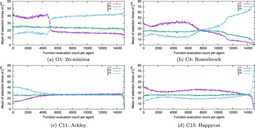
Next, we evaluated the transitions of the best function values obtained by four methods with $f_{max}=1200000$ for all 50-dimensional problems, and selected six typical results in them, which are shown in Figure 4. In the figures, its horizontal axis denotes the function evaluation count per agent, and its vertical axis does the mean of the best function values in the search process of each method on 50 trials. Finally, we focus on the number of times ${\mathit{\xi }}^{(k,i)}(t+1)$, $k\in \{1,2,3\}$ is selected in (22(22) $\begin{array}{rl}& {\mathit{x}}^{\left(i\right)}(t+1)\\ & =\mathrm{argmin}\left\{f\right(\mathit{x})|\mathit{x}\in \left\{{\mathit{\xi }}^{(1,i)}\right(t),{\mathit{\xi }}^{(2,i)}(t),{\mathit{\xi }}^{(3,i)}(t\left)\right\}\}.\end{array}$(22) ) of GWO-AS at iteration t + 1 as follows: $W^{\left(k\right)}(t+1):=\{i\in W|{\mathit{x}}^{\left(i\right)}(t+1)={\mathit{\xi }}^{(k,i)}\left(t\right)\},k\in \{1,2,3\}$, and compare the mean of $\left|W^{\left(k\right)}\right(t+1\left)\right|$ on 50 trials at each iteration in GWO-AS for four typical results, which are shown in Figure 5.

Figure 4. Means of the best function values obtained by four methods, PSO, FA, GWO-SR and GWO-AS, until function evaluation count per agent for 50-dimensional six benchmark problems.

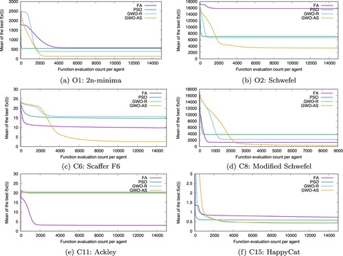
Figure 5. Means of $\left|W^{\left(k\right)}\right(t+1\left)\right|$, $k\in \{1,2,3\}$ for three candidates on 50 trials at each count when GWO-AS is applied to 50-dimensional four benchmark problems.

6.2. Discussion of results

First of all, we discuss obtained function values by four methods, as shown in Tables 4 and 5. Now, comparing the results of four methods and the original GWO with $\rho \ne 0$, which are shown in Table 2, we can see that four methods obtained better solutions than the original GWO with $\rho \ne 0$ for many problems, especially, GWO-SR and GWO-AS did. These results well demonstrate the disadvantages of the original GWO and the advantages of GWO-SR and GWO-AS. Next, concerning the comparison of three methods, PSO, FA and GWO-SR, the number of the problems for which the least objective functions was obtained by three methods are almost the same, which indicates that GWO-SR is not only invariant to shift-transformations by just introducing the reference point, but also has a similar search ability to other two methods. In addition, let us compare four methods, PSO, FA, GWO-SR and GWO-AS. From the above two tables, we can see that GWO-AS has better search ability than other three methods: GWO-AS obtained the first least function value for ten or eleven problems, and the second least function value for five ones in four methods. From these results, we can conclude that even though the GWO has serious drawbacks, the drawbacks can be overcome by applying the proposed methods, which implies that the basic concept for search in GWO is still promising, comparing other metaheuristic methods.

Secondly, we focus on the two proposed methods, GWO-SR and GWO-AS. From preparatory experiments for the methods with different reference points, which are shown in Tables 3 for GWO-SR, we observed that the appropriate reference points for GWO-SR were ${\mathit{\mu }}^{\left(1\right)}$ and ${\mathit{\mu }}^{(1,2)}$, while those for GWO-AS were ${\mathit{\mu }}^{\left(2\right)}$ and ${\mathit{\mu }}^{(2,1)}$, respectively. It means that the pbests are effective as the reference point for the search in GWO-SR, while the three best solutions are effective in GWO-AS. The difference can be attributed to the different search characteristics of the two methods. Although GWO-AS using the three best solutions may enhance the intensive search too strongly than GWO-SR, the balance between diversification and intensification is considered to be kept due to the proposed adaptive selection and mutation. Moreover, GWO-AS has better performance than GWO-SR in Tables 4 and 5, which indicates that the two proposed methods,the adaptive selection of search areas and the mutation procedure, are effective.

Thirdly, we discuss the relationship between computational complexity and search ability. In Figure 4, we can observe that all four methods decrease the objective function values sequentially as the search progresses. On the other hand, in the early stage of the search, the GWO-AS decreases more slowly than others, where the slow decline can be explained by the fact GWO-AS requires three times more function evaluations per iteration than the others, as mentioned previous section, while in the middle to end of the search, the GWO-AS decreases the function value significantly faster for many problems. In addition, as discussed above, the final function value obtained by GWO-AS was the least for many problems. These results suggest that the performance of search ability of GWO in terms of computational complexity is higher than others.

Finally, we analyze the mean of selection times of ${\mathit{\xi }}^{(k,i)}\left(t\right)$ per each count in GWO-AS, as shown in Figure 5, in which we can see that three kinds of candidates ${\mathit{\xi }}^{(k,i)}\left(t\right)$, $k\in \{1,2,3\}$ are variously selected as the search progresses: The candidate ${\mathit{\xi }}^{(k,i)}\left(t\right)$ which is most often selected is different in the first and second halves of the search, and its switching count is between 5000 and 8000. In the first half of the search, ${\mathit{\xi }}^{(1,i)}\left(t\right)$ with $c_1=3$ was most often selected, which is relatively small, while in its second half, ${\mathit{\xi }}^{(3,i)}\left(t\right)$ with $c_3=6$ was most often selected. From these results, we can see that three kinds of search areas are adaptively selected in GWO-AS for each problem as the search progresses.

7. Conclusion

In this paper, we have theoretically shown that the original GWO relies on a shift transformation of the problem, and have experimentally shown that its search is too specialized for problems with an optimal solution at the origin, which can significantly reduce its effectiveness of the search for other problems.

Next, we have proposed a modified method of GWO-R (GWO-SR) that is not only invariant to shift-transformations, and that can adjust reasonably its search areas. In addition, we have experimentally shown that its search area can be appropriately varied as the search progresses, in which GWO-SR is more efficient than GWO-R, and as efficient as PSO and FA. Moreover, we have proposed the GWO-AS by adding two methods, an adaptive selection method of the size of search area and a mutation procedure, to GWO-SR. Through numerical experiments, we have verified that the GWO-AS outperforms other methods. From these results, we can conclude that the basic concept of the search inspired by the hunting mechanism of grey wolves is promising despite of its serious drawbacks of the orignal GWO because the drawbacks can be easily overcome by the proposed methods.

Furthermore, since various methods have been investigated for the original GWO [3–8], the proposed GWO can be also modified by some of them. As a future issue, the performance evaluation of the proposed GWOs with such modifications should be verified. In addition, note that the whale optimization algorithm (WOA) [24], which is also one of the popular metaheuristic methods, uses basically the same update systems as the GWO. Thus, the method has the same drawbacks, as mentioned in Ref. [15]. It is possible to add the shift-invariance to WOA and modify its search ability as a general-purpose metaheuristic method by applying the methods used in GWO-SR and GWO-AS. Therefore, we would like to verify how useful those methods are when they are applied to the WOA, or what variations are particularly effective.

Disclosure statement

No potential conflict of interest was reported by the author(s).

Additional information

Notes on contributors

Keiji Tatsumi

Keiji Tatsumi, received the Ph. D. degree from Kyoto University, Japan, in 2006. In 1998, he joined Osaka University, where he is currently an Associate Professor of the Graduate School of Engineering. His research interests comprise metaheuristics for global optimization and machine learning.

Nao Kinoshita

Nao Kinoshita, received his M.S. degrees from Osaka University, Japan, in 2022. He is currently working for Nippon Steel Corp. His research interests are in metaheuristics for global optimization.

References

- Mirjalili S, Mirjalili SM, Lewis A. Grey wolf optimizer. Adv Eng Softw. 2014;69:46–61. doi: 10.1016/j.advengsoft.2013.12.007
- Muro C, Escobedo R, Spector L, et al. Wolf-pack (Canis lupus) hunting strategies emerge from simple rules in computational simulations. Behav Processes. 2011;88:192–197. doi: 10.1016/j.beproc.2011.09.006
- Mosav SK, Jalalian E, Gharahchopog FS. A comprehensive survey of grey wolf optimizer algorithm and its application. Int J Adv Robot & Expert Syst (JARES). 2018;1(6):23–45.
- Faris H, Mirjalili S. Grey wolf optimizer: a review of recent variants and applications. Neural Comput Appl. 2018;30:413–435. doi: 10.1007/s00521-017-3272-5
- Panda M, Dan B. Grey wolf optimizer and its applications: a survey. In: Proceedings of the Third International Conference on Microelectronics, Computing and Communication Systems. 2019.p. 179–194.
- Ali S, Sharma A, Jadon S. A survey on grey wolf optimizer. J Emerg Technol Innov Res (JETIR). 2020;7(11):789–790.
- Almufti SM, Ahmad HB, Marqas RB, et al. Grey wolf optimizer: overview, modifications and applications. Int Res J Sci Technol Educ Manage. 2021;1(1):44–56.
- Wu G, Mallipeddi R, Suganthan P. Ensemble strategies for population-based optimization algorithms – A survey. Swarm Evol Comput. 2019;44:695–711. doi: 10.1016/j.swevo.2018.08.015
- Mirjalili S. How effective is the grey wolf optimizer in training multi-layer perceptrons. Appl Intell. 2015;43:150–161. doi: 10.1007/s10489-014-0645-7
- Muangkote N, Sunat K, Chiewchanwattana S. An improved grey wolf optimizer for training q-Gaussian Radial Basis Functional-link nets, 2014 International Computer Science and Engineering Conference (ICSEC); 2014.
- Saremi S, Mirjalili SZ, Mirjalili SM. Evolutionary population dynamics and grey wolf optimizer. Neural Comput Appl. 2015;26:1257–1263. doi: 10.1007/s00521-014-1806-7
- Shankar K, Eswaran P. A secure visual secret share (VSS) creation scheme in visual cryptography using elliptic curve cryptography with optimization technique. Aust J Basic Appl Sci. 2015;9(36):150–163.
- Jian Z, Zhu G. Affine invariance of meta-heuristic algorithms. Inf Sci (Ny). 2021;576:37–53. doi: 10.1016/j.ins.2021.06.062
- Niu P, Niu S, Liu N, et al. The defect of the grey wolf optimization algorithm and its verification method. Knowl Based Syst. 2019;171:37–43. doi: 10.1016/j.knosys.2019.01.018
- Askari Q, Younas I, Saeed M. Emphasizing the importance of shift invariance in metaheuristics by using whale optimization algorithm as a test bed. Soft Comput. 2021;25:14209–14225. doi: 10.1007/s00500-021-06101-9
- Tatsumi K, Kinoshita N. Shift-invariant grey wolf optimizer exploiting reference points and random selection of step-sizes. Proc SICE Ann Conf. 2022;2022:1201–1206.
- Kennedy J, Eberhart RC. Particle swarm optimization. Proc IEEE Int Jt Conf Neural Netw. 1995;4:1942–1948.
- Poli R, Kennedy J, Blackwell T. Particle swarm optimization – an overview. Swarm Intell. 2007;1:33–57. doi: 10.1007/s11721-007-0002-0
- Yang XS. Nature-Inspired metaheuristic algorithms. Frome: Luniver Press; 2008.
- Fister I, Fister J.I, Yang XS, et al. A comprehensive review of firefly algorithms. Swarm Evol Comput. 2013;13:34–46. doi: 10.1016/j.swevo.2013.06.001
- Grey Wolf Optimizer (GWO) version 1.6 (1.85 MB) by Mirjalili S. GWO is a novel meta-heuristic algorithm for global optimization. https://www.mathworks.com/matlabcentral/fileexchange/44974-grey-wolf-optimizer-gwo.
- Awad NH, Ali MZ, Suganthan PN, et al. Problem definitions and evaluation criteria for the CEC 2017 special session and competition on single objective real-parameter numerical optimization, Technical Report of Nanyang Technological Univ., Jordan Univ. and Zhengzhou Univ., 2016.
- Clerc M. Particle swarm optimization. London: ISTE Publishing; 2006.
- Mirjalili S, Lewis A. The whale optimization algorithm. Adv Eng Softw. 2016;95:51–67. doi: 10.1016/j.advengsoft.2016.01.008