High precision localization for periodic tunnel inspections

Abstract

In tunnel inspections, it is important to check for the progression of cracks and other deformations. The point clouds of tunnels are not reproducible due to accumulated errors in mobile mapping systems using GNSS/IMU navigation. Therefore, it has been impossible to confirm the progression of deformations with the original point cloud because the shapes of the acquired point clouds do not match. Therefore, the position of the point cloud has been corrected by surveying or by manual alignment of the point cloud. This was time-consuming and costly. In this paper, we propose a new positioning method for two-time difference comparisons based on a scan-matching technique that matches tunnel features and describe the evaluation results. The results of evaluation experiments show that the average error before alignment was 0.831 m. The proposed method achieves alignment with an average error of less than 0.040 m, which is unprecedentedly accurate.

KEYWORDS:

• Tunnel inspection
• localization in GNSS invisible environment
• scan matching
• mobile mapping system
• point cloud

1. Introduction

Japan’s topography is rugged, with mountainous terrain covering approximately 75% of the country. For this reason, 10,000 road tunnels have been constructed in Japan as of 2022. By 2033, about 42% of these tunnels will be more than 50 years old. Therefore, periodic inspections of tunnels are conducted every five years to maintain the infrastructure.

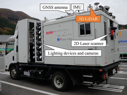
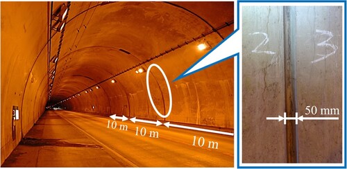
Although periodic inspections have traditionally involved close visual inspection of the entire tunnel and full-surface sound inspections, manpower shortages and cost issues have created a need for more efficient inspections through pre-screening and alternative methods. Among them, an inspection using a Mobile Mapping System (MMS), in which sensors are mounted on the vehicle without the need for traffic control, has been proposed, as shown in Figure 1. These systems include the Mobile Imaging Technology System, which uses multiple cameras mounted on the sides of the vehicle to collect images of the tunnel lining surface, and the Mobile Laser Scanning System, which uses a laser scanner to measure the shape of the tunnel. In inspections using these systems, it is important to compare past and current inspection results to determine the progression of tunnel deformations. Since comparison of inspection results is based on location information, experience has shown that the precision of MMS localization should be within 5 cm. Most MMS used for tunnel inspections are equipped with a GNSS/IMU combined navigation system as a localization device. However, GNSS/IMU combined navigation is a system that reduces the cumulative error of IMU dead reckoning by periodically observing GNSS. Therefore, in tunnels where GNSS is not available for long periods of time, errors accumulate. For example, it is known that if GNSS is unavailable for 75 s, an error of more than 1 m will occur at the centre of the tunnel [1]. Therefore, there is a need for a method for highly accurate localization in tunnels where GNSS cannot be used.

Figure 1. MMS for tunnel inspection.

There are already several localization methods that do not use GNSS. Among them, we have developed a 3D LiDAR scan matching method that extracts lighting as a feature in tunnels and uses it as a landmark, as a method that does not require construction of equipment in tunnels and is easy to integrate into existing MMS [2]. Although this method has shown a certain level of precision improvement, the location and shape of lighting and other ancillary equipment are replaced every few years, and their installation positions and shapes may differ each time they are periodically inspected. Therefore, they are not suitable as features in tunnels. In the conference paper [3] presented at the SICE Annual Conference 2023, we proposed a localization method that selects alternative features to lighting and uses scan matching with features in the tunnel.

This paper is a revised version of that conference paper, with the following changes.

1. Added explanations about the results of validation using existing methods and about the hardware.

2. Implemented multiple types of filters and compared their accuracies.

3. Visualized the errors of all points and evaluated the presence of minor distortions.

4. Modified the procedures for sensor calibration and scan matching.

For I–III, additional descriptions and discussions were made on the points that were not sufficiently explained or evaluated in the conference paper.

For IV, the method in the conference paper directly registers a 3D LiDAR point cloud with a measurement precision of ±15 mm and an MMS point cloud with a measurement precision of ±0.3 mm, and the final precision is affected by the error of the 3D LiDAR. The new method unifies the point clouds of MMS with the same measurement precision, thereby improving precision.

In the method described in the conference paper, the sensor calibration and scan matching procedures are separated, and the positional calibration of the 3D LiDAR and 2D laser scanner is performed only once at the beginning of the process. On the other hand, this method recalculates the positional relationship between the 3D LiDAR and 2D laser scanner after each of the above registration steps. This method is also meant to compensate for the synchronization error between the sensors, which cannot be perfectly synchronized by the sensor synchronization method described below.

2. Related works

Many methods of localization in environments where GNSS is not available have already been studied. One method used in MMS is to correct the position by manually specifying a previously surveyed point as a correction point [4]. This method is also used in current position correction in tunnels, but it requires separate surveying, which is costly and time-consuming, and diminishes the advantages of mobile measurement.

There are also methods using pseudolite [5,6] and Wi-Fi [7,8]. However, these methods have the fundamental problem that multipath and reflections of radio waves from surrounding walls make accurate localization difficult. Although several multipath and noise suppression algorithms have been proposed in recent literature, such algorithms are complex and require high processing power. In addition, the cost of installing and maintaining equipment for each tunnel is a significant challenge in situations such as tunnel inspections.

There are several methods for localization that do not require new infrastructure facilities, such as Simultaneous Localization and Mapping (SLAM) and scan matching, which is a localization method for a pre-made map. In SLAM, the amount of movement is sequentially estimated by matching point clouds, and self-localization is estimated by adding up the amount of movement. There are two types of this: visual-based [9,10] and LiDAR-based [11–14], with LiDAR-based methods generally being more accurate. One method suitable for LiDAR is Laser Odometry and Mapping (LOAM), which extracts feature points on edges and points on planes from a point cloud and uses them for registration [11,12].

Scan matching with LiDAR point clouds uses the Iterative Closest Point (ICP) algorithm [15], which determines and minimizes the sum of squares of distances between point clouds, and the Normal Distributions Transform (NDT) algorithm [16], which divides the search space into grids and optimizes alignment. Filter processing for nonlinear data, such as particle filters (PF), extended Kalman filters (EKF), and unscented Kalman filters (UKF), are often used to smooth scan-matching results and fuse them with other sensor data [17–22]. These methods are extensively used to estimate the self-position of mobile objects. For instance, the studies in [23,24] use ground vehicles to update 3D maps of human living environments. In contrast, the works presented in [25,26] employ UAVs for localization and mapping.

On the other hand, it is known that in places where the same shape continues in the travel direction, such as a tunnel or a corridor in a building, it is not easy to align the point clouds in the travel direction [13,14]. Therefore, the shape of tunnels breaks down when using existing SLAM public packages, as shown in Table 1.

Table 1. Localization in tunnel using SLAM.

To address this problem, our previous work proposed scan matching with extracted lighting as a feature. As a result, Root Mean Square Error (RMSE) was estimated to be within 0.2 m in all xyz-axis directions [2]. In addition, Kyuwon Kim et al. proposed a method to compensate for positional errors based on the location of detected hydrants and lanes. As a result, RMSE was estimated to be within 0.2 m both laterally and longitudinally of the lane [27]. These studies have shown the effectiveness of localization with features in tunnels method, but the precision of the method is insufficient for use in inspections. In addition, ancillary equipment is not suitable as a feature for localization because it is replaced every few years. This work proposes a method to solve these problems.

3. Methods

The method proposed in this work assumes that a high-precision point cloud of the tunnel is created in advance by combining surveying with the first measurement of the tunnel’s 3D geometry. Hereafter, the collective point cloud of the entire tunnel obtained through inspection is denoted as M_n, where the subscript n indicates the number of inspections. In this system, the point cloud M₁ measured during the first inspection is used as the reference. For subsequent inspections, the location of the measured point cloud M₂ is corrected, and the progression of anomalies is determined based on their correspondence. This method proposes a highly accurate localization technique through scan matching that extracts features in the tunnel with minimal long-term changes and uses them as landmarks. This approach enables high-precision localization during regular inspections without the need for new infrastructure installation in the tunnel or manual correction work.

This chapter provides a detailed explanation of the proposed positioning method.

3.1. Hardware configuration

3.1.1. Mobile mapping system

This section describes the MMS used for the verification of this method. The MMS used in this method is a measurement vehicle known as MIMM. It combines two-dimensional point clouds measured by a 2D laser scanner with positional information obtained from a GNSS/IMU combined navigation system, enabling the reconstruction of three-dimensional point clouds.

The 2D laser scanner equipped on the MMS rotates at 200 Hz and can measure a grey object at a distance of 5 metres with an accuracy of 0.3 mm, capturing one million points per second. The measurement density varies with the travel speed. In the travel direction, points are measured at intervals of 5.5 cm at a speed of 40 km/h, while in the transverse direction, the intervals vary depending on the tunnel radius. However, for a tunnel with a radius of about 6 metres, the measurements are taken at approximately 7 mm intervals. Table 2 shows the specifications of each device mounted on MIMM.

Table 2. Specifications of devices on MIMM.

Device name	Specification
2D laser scanner (S-2100)	Data acqusition rate: 1,016,000 points/sec.
	Range: 119 m
	Rotation speed: 200 Hz
	Resolution range: 0.1 mm
	Accuracy (1σ): 0.3 mm (Target distance 5 m, Intensity >37%)
GNSS	3 units (1 dual-frequency, 2 single-frequency)
IMU	3-axis FOG, 3-axis accelerometer

3.1.2. Synchronization system for localization sensors

Figure 2 shows the system configuration, and Figure 3 shows the appearance of the added hardware. In this method, 3D LiDAR and GNSS are additionally mounted on the existing MMS. The GNSS used in this system is not for localization, but as a system for time synchronization between sensors. Time synchronization between sensors is important for improving the precision of localization and 3D reconstruction. Normally, it is desirable to synchronize within a single measurement system, but since this system is a device additionally installed on the existing MMS, the measurement system is divided into multiple parts. Therefore, it is necessary to synchronize the time between different systems.

Figure 2. Synchronization system for localization sensors.

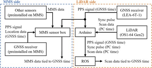
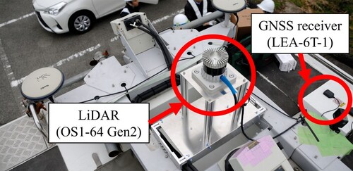
Figure 3. Appearance of the added hardware.

The existing MMS records the time of each sensor based on GNSS time. This time synchronization system uses the Pulse Per Second (PPS) signal output from the GNSS receiver, and synchronization is maintained using the PPS signal even when GNSS cannot be received. Therefore, it is desirable for this system to also record sensor time based on GNSS time, aligning with MMS practices. For this reason, in this system, time synchronization is achieved by branching the GNSS’s PPS signal to both the MMS and this system. This approach parallels the method proposed by L. Mengtong et al. [28].

The specifications of the 3D LiDAR used in this system are shown in Table 3. This 3D LiDAR emits 64 lasers simultaneously and is a sensor that can measure the 3D shape around LiDAR all at once. In this method, the point cloud obtained from this 3D LiDAR is used for position estimation. The sensor rotates at 10 Hz and can measure about 1.3 million points per second with 64 lasers. The measurement density is approximately 3.8 cm intervals on the tunnel wall directly beside the sensor in the rotational direction, and 5 cm intervals in the vertical direction. The measurement accuracy is within ±15 mm distance error. Therefore, compared to the laser mounted on the MMS, the density and accuracy of the point cloud are lower. Hereafter, the collection of point clouds measured by the 3D LiDAR will be denoted as ${\mathbf{s}}_{\mathbf{n}}{\mathbf{=}\{\mathbf{s}}_{\mathbf{n}}^{\mathbf{1}}{\mathbf{,}\mathbf{s}}_{\mathbf{n}}^{\mathbf{2}}{\dots \mathbf{s}}_{\mathbf{n}}^{\mathbf{t}}{\mathbf{,}\mathbf{s}}_{\mathbf{n}}^{\mathbf{t}\mathbf{+}\mathbf{1}}\dots \}$. s_n represents all the point clouds of the 3D LiDAR measured during the n-th inspection. ${\mathbf{s}}_{\mathbf{n}}^{\mathbf{t}}$ represents the collection of one rotation’s worth of point clouds acquired at the time t during the n-th measurement.

Table 3. Specifications of 3D LiDAR (OS1-64 Gen2).

Number of channels (vertical)	64
Resolution (horizontal)	1024
Viewing angle (vertical)	33.2° (±16.6°)
Angular resolution (vertical)	0.53°
Range	120 m
Precision	±15 mm
Rotation speed	10 Hz
Data acqusition rate	1,310,720 points/sec

3.2. Localization method using tunnel features based scan matching

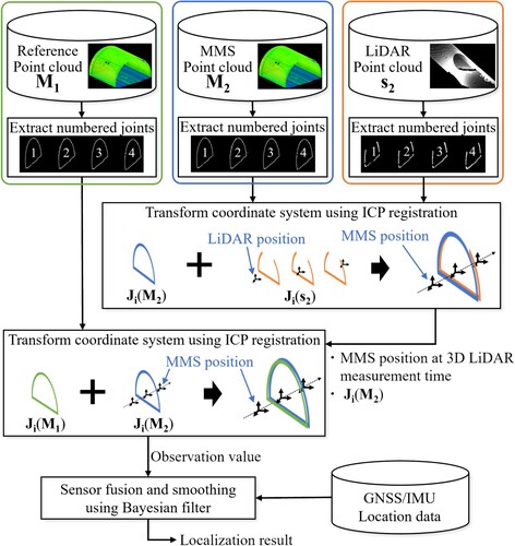
The flow of the proposed method is shown in Figure 4. First, tunnel-specific features are extracted from each of the point clouds M₁, M₂ and s₂. Then, the point clouds are aligned with each other using ICP matching based on the positional relationship of the features.

Figure 4. Flow of proposed localization method in tunnels.

3.2.1. Feature extraction from tunnel point clouds

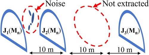
In this section, we describe the features in the tunnel used in the proposed method. There is much ancillary equipment in tunnels, such as jet fans, fire hydrants, emergency telephones, cables, and lighting and so on. However, most of the ancillary equipment is limited in quantity, and the cables are installed along the travel direction. Lighting, used as a feature in a previous work [2], is installed in large numbers in the tunnel. However, lighting is replaced every few years, and the location and placement of lighting may change with each periodic inspection. Therefore, we focused on the joints of blocks or segments in the tunnel structure, as illustrated in Figure 5. This seam is a shape feature that exists transversely along the inner wall of the tunnel and is present at regular intervals in the travel direction. Unlike other ancillary equipment, these cannot be replaced, making them suitable as a reference for comparing point clouds measured at different times. Hence, in this work, we utilize these joints as the features.

Figure 5. Example of joints in a tunnel.

In this method, the position and orientation of the newly measured point cloud M₂ are aligned with the previously measured point cloud M₁.

First, joint point clouds are extracted as features from all point clouds used for alignment. The point clouds used vary in point cloud density and measurement precision depending on the measurement device. Therefore, different methods need to be employed to extract features from each point cloud.

3.2.1.1. Feature extraction from high-precision and high-density point cloud

First, I will explain the details of the method for extracting features from the point cloud M_n measured by the MMS. The collection of feature point clouds extracted from M_n is denoted as J∈M_n, and hereafter referred to as J(M_n).

1. The point cloud is then moved to the origin using the following procedure, as shown in Figure 6.

Figure 6. Align point cloud to the XY plane.

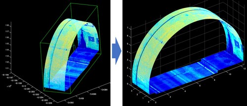
First, the tunnel point cloud is separated at regular intervals in the travel direction. Then, an Oriented Bounding Box (OBB) is calculated for the separated tunnel point cloud.

Then, rotate the point cloud around the z-axis so that the x-axis is in the travel direction crossing and the y-axis is in the travel direction using the calculated OBB end point coordinates. The Random Sample Consensus (RANSAC) and least squares methods were then used to detect the point cloud in the road surface area and to compute a planar model of the road surface. Finally, the planar model of the road surface is used to calculate the gradient of the road surface and the road surface is rotated and shifted so that it is in the by-plane.

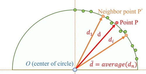
• If the points are a short distance apart in the direction of travel, the section can be considered a straight line. Therefore, when the tunnel wall is projected onto the oz. plane, the distance from the tunnel centre to the wall is approximately equidistant. On the other hand, the joints are grooved with respect to the wall surface, making the distance longer than the tunnel centre. Auxiliary facilities such as lighting and jet fans are also shorter distances from the tunnel centre. This feature is used to extract the joint point cloud.

The previous point cloud is projected onto the oz. plane. First, the road surface point cloud is removed and then the approximate circle of the point cloud on the tunnel wall is obtained using curve fitting. Next, the distance $d$ from the centre O of the approximate circle to a point P on a certain wall surface is determined. Then, the average distance $\overline{d}$ between the neighbouring points within a threshold from point P and the centre O is determined. The radius of the neighbourhood search is empirically set to 0.2 m. Points where the difference between d and the $\overline{d}$ is greater than the threshold are extracted as candidate points for ancillary equipment. The threshold is empirically set to 2 cm. Figure 7 shows an image of candidate point cloud extraction for ancillary equipment.

Figure 7. Extraction of candidate ancillary facility points.

The candidate points are a group of points away from the tunnel wall, include lights, cables and joints as shown in Figure 8.

Figure 8. Extracted ancillary equipment point cloud.

The joints are grooves perpendicular to the tunnel. Therefore, the point cloud of the joint can be extracted by using RANSAC to extract segments of the point cloud with a vertical linear component.

1. Joints extracted from the tunnel point cloud were extracted were returned to their original coordinates. Subsequently, the point clouds close to the xy-coordinates were extracted from the original point clouds and combined to obtain the road-surface point cloud. The final extraction results are shown in Figure 9.

2. As shown in Figure 10, for the extracted point cloud J(M_n), numbers i are assigned to the points in sequence starting from the mine entrance. This point cloud is denoted as J_i(M_n). Among the point cloud data extracted in the process up to step (iii), those that were equally spaced were treated as a joint, and the numbers were assigned in order starting from the one nearest to the entrance. If noise existed between the joints, it was eliminated; if a joint was not extracted, its number was skipped.

Figure 9. Joint extraction result from MMS point cloud.

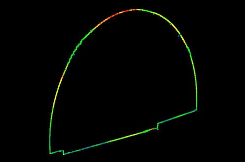
Figure 10. Assign numbers to joints in sequence.

3.2.1.2. Feature extraction from LiDAR point cloud

The point cloud s₂ measured by 3D LiDAR has a lower density compared to the point cloud M₂, making it difficult to perform feature extraction using the same method as in the previous section 3.2.1.1. Therefore, this section will describe the details of the method for extracting the feature point cloud J(s₂) from low-density and low-precision point clouds.

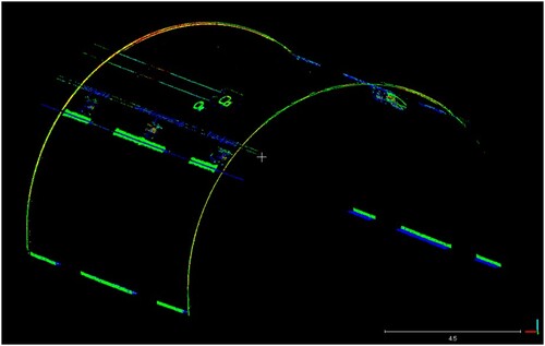
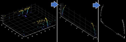
1. First, 3D LiDAR continuously measures the shape data of the entire 360-degree circumference at 10 Hz. From this data, one round of point cloud data is extracted as a single scan data, and the joint point cloud is extracted.

Figure 11 shows the point cloud of one scan of 3D LiDAR. The left side of Figure 11 shows the data acquired at the mine entrance, and there is a difference between the left and right point clouds. This is because it takes 0.1 s to acquire one scan of data, so for example, if the vehicle is travelling at a speed of 40 km/h, it will advance about 0.11 m. As a result, the point clouds are distorted. This results in distortion of the point clouds. The distortion of the point clouds are corrected by calculating the MMS measurement speed at each time from the odometry data. The right side of Figure 11 shows the corrected point cloud data, indicating that the distortion has been correctly corrected.

1. Next, the point cloud for one scan was divided into point clouds for each scan line. The LiDAR used in this work had 64 lines. Therefore, it was divided into 64 sections. A straight line was calculated that consisted of two points, P_i and P_i-1. Similarly, a line that consisted of two points, P_i and P_i+1, was calculated as show in Figure 12, and the cosine similarity was calculated based on the two lines. In this case, the calculation was not performed in 3D but in two dimensions (xy-plane). Threshold processing was applied to the calculated cosine similarity to extract areas with large curvature variations. The results are shown in Figure 13.

2. From the point cloud extracted in (ii), remove the road and ceiling point clouds based on their heights. Next, segment the point cloud of the wall surface using nearest neighbour search. An OBB is applied to each segment. Focusing on the height direction of each OBB, the segment with the longest OBB in the height direction is extracted as a candidate point cloud for the joint. Finally, RANSAC is applied to these candidate points to extract only the linear points that constitute the point cloud of the joint. The result is shown in Figure 14. ICP matching using only this joint point cloud results in circle-to-circle matching. Therefore, mismatching occurs in the roll direction. To prevent mismatching, a point cloud of the road surface on the same line as the joint is also extracted.

3. Finally, the extracted point cloud J(s₂) is assigned numbers starting from the tunnel entrance. At this time, the joint number i is determined by calculating the observation time t of J_i(M₂) based on the positional relationship between each sensor and the joint, the travel speed, and the measurement time of the 3D LiDAR. Number i is then assigned to J(s₂) measured in the vicinity of the same time.

Figure 11. Distortion correction.

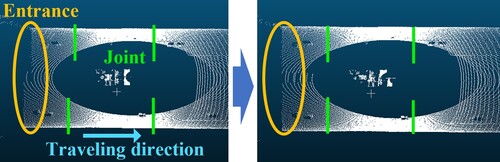
Figure 12. Curvature change point extraction per scan line.

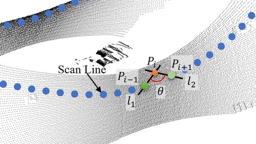
Figure 13. Thresholding based on cosine similarity.

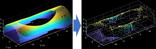
Figure 14. Joint extraction result from LiDAR point cloud.

3.2.2. Localization using joint point clouds

This section discusses a localization method using the joint point clouds extracted in the previous section. This method is an improvement on one previously proposed in a conference paper [3].

First, the point cloud J_i(M₂) measured by the MMS’s 2D laser scanner and the point cloud J_i(s₂), measured simultaneously with J_i(M₂) by the 3D LiDAR, are aligned. This alignment estimates the position of the MMS relative to J_i(M₂) at the time of the 3D LiDAR measurement, thereby correcting the positioning results obtained through MMS’s dead reckoning. At this point, the positional relationship between the 3D LiDAR and other sensors of the MMS has already been measured and calibrated.

Next, the point cloud J_i(M₂) is aligned with the previously measured point cloud J_i(M₁), which serves as a reference for the tunnel shape. This alignment estimates the position of the MMS relative to J_i(M₁). This estimated position is then input into a Bayesian filter as an observed value. The alignment in these processes employed registration using the ICP algorithm.

3.2.3. Smoothing using Bayesian filter

In this section, state estimates obtained by scan matching are smoothed using Bayesian filters [17–22].

In the conference paper [3], the g-h Filter was employed. While this method is simple and easy to implement, high precision cannot be expected. Therefore, in this paper, we applied the particle filter (PF), the extended Kalman filter (EKF), and the unscented Kalman filter (UKF), which can handle nonlinear data and are widely used in general, respectively, and compared their results. Additionally, in the g-h filter of conference paper [3], processing was conducted solely in time series order. Furthermore, when updating the state at a certain time t, the update was also reflected in the states following time t. However, in this paper, we unified all processing procedures except for the inherent processing of each filter in order to compare their precision. Therefore, the g-h filter in this paper is processed differently from the method used in the conference paper.

First, we explain the processing common to each filter. The state vector x at each time is defined as (1) $\mathit{x}=[\mathrm{xyz\varphi \theta \psi }{]}^T$(1) The observation vector $\mathit{z}$ obtained by scan matching is also defined in the same way. The control input $\mathit{u}$ consists of the linear and angular velocities obtained by the MMS navigation system and is defined as (2) $\mathit{u}=[v_x{v}_y{v}_z{\omega }_{\varphi }{\omega }_{\theta }{\omega }_{\psi }{]}^T$(2) The state at each time is estimated through the processing of the prediction and update steps by each method. This is done from both the time-series and reverse time-series order of the data, and the results are integrated. As an integration method, the later in the filtering process, the higher the confidence level.

Next, the processing specific to each filter is explained.

3.2.3.1. g-h filter

The g-h filter does not require a detailed system model.

In the prediction step, the current estimated state $\mathit{x}$, the control input $\mathit{u}$, and the time interval $\mathrm{\Delta t}$ are used to compute a time-evolved prediction vector $\overline{\mathit{x}}$, instead of using a scaling factor h for changes in the observed values as in the usual g-h filter. (3) $\overline{\mathit{x}}=\mathit{x}+\mathit{u}\mathrm{\Delta t}$(3) In the update step, the state vector $\mathit{x}$ is updated using the observation vector $\mathit{z}$, the prediction vector $\overline{\mathit{x}}$, and the scaling factor $g$ for the observations. (4) $\mathit{x}=\overline{\mathit{x}}+g\left(\mathit{z}-\overline{\mathit{x}}\right)$(4) The above is the g-h filter process.

3.2.3.2. Particle filter

PF does not assume an error distribution as such, but instead generates several hypotheses of states, called particles, and calculates the robot’s position based on the distribution of these hypotheses.

In the prediction step, the prediction vector $\overline{\mathit{x}}$ of each time-evolved particle is computed using the current estimated state $\mathit{x}$, the control input $\mathit{u}$, the time interval $\mathrm{\Delta t}$, and the motion noise $ϵ$ according to the covariance matrix $\mathit{Q}$. (5) $\overline{\mathit{x}}=\mathit{x}+\mathit{u}\mathrm{\Delta t}+ϵ$(5) In the update step, the weight of each particle is calculated, and the particles are resampled based on this weight. The weights are based on the agreement between the particle’s predicted state $\overline{\mathit{x}}$ and the observed value $\mathit{z}$. If the weight of particle $k$ is ${\mathit{w}}_k$ and the observed noise variance according to the covariance matrix R is ${\sigma }^2$, the weight calculation follows the formula. (6) ${\mathit{w}}_k={\mathit{w}}_k\frac{1}{\sqrt{2\pi {\sigma }^2}}\text{exp}\left(-\frac{{\left(\overline{\mathit{x}}-\mathit{z}\right)}^2}{2{\sigma }^2}\right)$(6) calculate the effective sample size $N_e$ and perform resampling if it is below the threshold. The number of particles is $N_p$ and the weight of each particle ${\overline{\mathit{x}}}_i$ is ${\mathit{w}}_{\mathit{i}}$. Resampling was performed using the low variance sampling algorithm. (7) $N_e=\frac{1}{{\sum }_{i=1}^{N_p}{\left({\mathit{w}}_i\right)}^2}$(7) Compute the updated estimated state $\mathit{x}$ using the weights of each particle. (8) $\mathit{x}=\sum _{i=1}^{N_p}{\overline{\mathit{x}}}_i{\mathit{w}}_i$(8) The above is the g-h filter process.

3.2.3.3. Extended Kalman filter

EKF is a nonlinear version of the Kalman filter that linearizes the current mean and covariance estimates. The EKF is widely used in systems that perform nonlinear state estimation.

In the prediction step, when the control input is $u$ and the current estimated state is $\mathit{x}$, the predicted state is $\overline{\mathit{x}}$ computed using the nonlinear function $f$. (9) $\overline{\mathit{x}}=f\left(\mathit{x},\mathit{u}\right)$(9) The error covariance matrix $\mathit{P}$ represents the uncertainty in the state estimation. The prediction $\overline{\mathit{P}}$ of the error covariance matrix is computed using the Jacobi matrix $\mathit{F}$, the process noise covariance matrix $\mathit{Q}$. This Jacobi matrix is used to linearize the motion model. (10) $\overline{\mathit{P}}=\mathit{FP}{\mathit{F}}^T+\mathit{Q}$(10) In the update step, the covariance matrix S of the observed residuals is first calculated using the Jacobi matrix H of the observation model, the observed noise covariance R, and the prediction error covariance matrix $\overline{\mathit{P}}$.

The Kalman gain K is then computed. (11) $\begin{array}{rl}& \mathit{S}=\mathit{H}\overline{\mathit{P}}{\mathit{H}}^T+\mathit{R}\end{array}$(11) (12) $\begin{array}{rl}& \mathit{K}=\overline{\mathit{P}}{\mathit{H}}^T{\mathit{S}}^{-1}\end{array}$(12) Finally, the nonlinear function h is used to compute the residuals of the observations and update the state estimate x and the error covariance matrix P. (13) $\begin{array}{rl}& \mathit{x}=\overline{\mathit{x}}+K\left(\mathit{z}-h\left(\overline{\mathit{x}}\right)\right)\end{array}$(13) (14) $\begin{array}{rl}& \mathit{P}=\left(\mathit{I}-\mathit{KH}\right)\overline{\mathit{P}}\end{array}$(14) The above is the EKF process.

3.2.3.4. Unscented Kalman filter

UKF, like EKF, is used for nonlinear state estimation. However, UKF does not linearize the nonlinear function itself. Some representative points (sigma points) representing the state distribution are propagated directly through to the nonlinear function. It then uses the mean and covariance estimated from the results.

The prediction step first generates sigma points ${\mathit{X}}_i$ to approximate the nonlinear dynamics of the system. In the n-dimensional Gaussian distribution of the mean $\mu$ and covariance $\mathbf{\Sigma }$, the following equation is obtained. (15) $\begin{array}{rl}& \lambda ={\alpha }^2\left(n+\kappa \right)-n\end{array}$(15) (16) $\begin{array}{rl}& {\mathit{X}}_0=\mu \end{array}$(16) (17) $\begin{array}{rl}& {\mathit{X}}_i=\mu +{\left[\sqrt{\left(n+\lambda \right)\mathrm{\Sigma }}\right]}_i\text{for}i=1,\dots ,n\end{array}$(17) (18) $\begin{array}{rl}& {\mathit{X}}_i=\mu -{\left[\sqrt{\left(n+\lambda \right)\mathrm{\Sigma }}\right]}_{i-n}\text{for}i=n+1,\dots ,2n\end{array}$(18)

In these equations, the subscript I denotes the itch row vector of the matrix. $\alpha$ and $\kappa$ are scaling parameters that determine how far away from the centre the sigma points are chosen. Two weights are associated with each sigma point ${\mathit{X}}_i$. ${\mathit{w}}_0^m$ is used when computing the mean, and $w_0^c$ is used when computing the covariance. These weights are defined as follows, (19) $\begin{array}{rl}& {\mathit{w}}_0^m=\frac{\lambda }{n+\lambda }\end{array}$(19) (20) $\begin{array}{rl}& {\mathit{w}}_0^c=\frac{\lambda }{n+\lambda }+\left(1-{\alpha }^2+\text{β}\right)\end{array}$(20) (21) $\begin{array}{rl}& {\mathit{w}}_0^m={\mathit{w}}_0^c=\frac{\lambda }{2\left(n+\lambda \right)}\text{for}i=1,\dots ,2n\end{array}$(21) In this equation, $\text{β}$ is a parameter to reflect the knowledge about the distribution, which is approximated by a Gaussian distribution. Each sigma point is then passed to the function f. The sigma points are projected by the process model to the next time and constitute a new prior distribution. Let Y be the set of sigma points after passing through f. (22) $\mathit{Y}=f\left(\mathit{X}\right)$(22) Compute the mean $\overline{\mathit{x}}$ and covariance matrix $\overline{\mathit{P}}$ of the prior distribution with the unscented transform for the transformed sigma points. (23) $\begin{array}{rl}& \overline{\mathit{x}}=\sum _{i=0}^{2n}{\mathit{w}}_i^m{\mathit{X}}_i\end{array}$(23) (24) $\begin{array}{rl}& \overline{\mathit{P}}=\sum _{i=0}^{2n}{\mathit{w}}_i^c\left({\mathit{X}}_i-\overline{\mathit{x}}\right)({\mathit{X}}_i-\overline{\mathit{x}}{)}^T+\mathit{Q}\end{array}$(24) In the update step, the sigma points Y representing the prior distribution are first transferred to the observation space by the observation function h. Let Z be the set of sigma points Y after passing through h. (25) $\mathit{Z}=h\left(\mathit{Y}\right)$(25) From here, the mean ${\mathit{\mu }}_z$ and the covariance matrix ${\mathit{P}}_z$ are calculated using the unscented transform. The subscript z denotes the transfer to the observation space. (26) $\begin{array}{rl}& {\mathit{\mu }}_z=\sum _{i=0}^{2n}{\mathit{w}}_i^m{\mathit{Z}}_i\end{array}$(26) (27) $\begin{array}{rl}& {\mathit{P}}_z=\sum _{i=0}^{2n}{\mathit{w}}_i^c\left({\mathit{Z}}_i-{\mathit{\mu }}_z\right)({\mathit{Z}}_i-{\mathit{\mu }}_z{)}^T+\mathit{R}\end{array}$(27) The calculation of the Kalman gain requires the mutual covariance ${\mathit{P}}_{\mathrm{xz}}$ of the states and observables. This is defined as (28) ${\mathit{P}}_{\mathrm{xz}}=\sum _{i=0}^{2n}{\mathit{w}}_i^c\left({\mathit{Y}}_i-\overline{\mathit{x}}\right)({\mathit{Z}}_i-{\mathit{\mu }}_z{)}^T$(28) The Kalman gain K is defined as (29) $\mathit{K}={\mathit{P}}_{\mathrm{xz}}{\mathit{P}}_z^{-1}$(29) Finally, the new state estimate x and covariance P are computed by the following equation, (30) $\begin{array}{rl}& \mathit{x}=\overline{\mathit{x}}+\mathit{K}\left(\mathit{z}-{\mathit{\mu }}_z\right)\end{array}$(30) (31) $\begin{array}{rl}& \mathit{P}=\overline{\mathit{P}}-\mathit{K}{\mathit{P}}_z{\mathit{K}}^T\end{array}$(31) The above is the UKF process.

4. Evaluation test of the proposed method

4.1. Outline of the experiment

To evaluate the performance of the method, an experiment was conducted using an actual tunnel. Figure 15 shows the experimental environment.

Figure 15. Experimental environment.

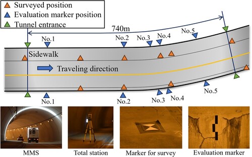
The measured tunnel has a total length of 740 m and Cannot see both entrances from inside the tunnel. There is also a sidewalk along the side of the road. Eight evaluation markers were placed in the tunnel for evaluation purposes, and seven other evaluation markers were placed for surveying purposes. MMS was used to measure the tunnel multiple times at a speed of 40 km/h, all on the same day. Therefore, the shape of the tunnel remains unchanged.

In this work, one of these measurements was used as the point cloud M₁, and the other measurements were assumed to be the point cloud after the inspection. Tunnel data used for the point cloud M₁ is position-corrected in advance using the method of Sakuma et al. [4], using survey marker positions. This experiment compares the precision before and after applying the proposed method. In addition, the performance of different Bayesian filters is also evaluated. Two methods were used to evaluate the precision of the location estimation results.

4.2. Precision evaluation using markers

For the first evaluation method, the evaluation markers shown in the lower row of Figure 15 were placed at the blue triangles in the tunnel. The evaluation marker can be clearly recognized on the point cloud because the laser reflection intensity is very different from the surrounding wall surface. The evaluation marker positions in the uncorrected point cloud M₂ and the corrected point cloud M’₂ groups were compared with the evaluation marker positions in the point cloud M₁, respectively. Figure 16 shows a comparison of evaluation markers. The positions of the evaluation markers in the point cloud M₁ and the position errors in the uncorrected point cloud M₂ and the corrected point cloud M’₂ are shown in Table 4.

Figure 16. Comparison of evaluation marker positions.

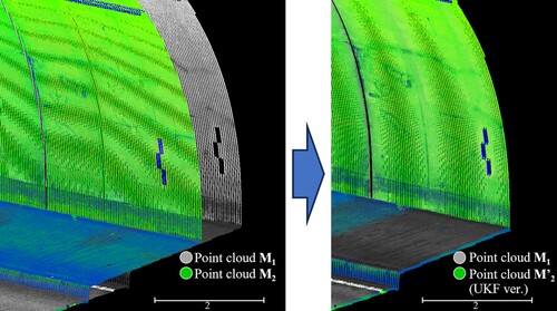
Table 4. Error comparison before and after correction.

No.	Uncorrected (m)	g-h F (m)	PF (m)	EKF (m)	UKF (m)
1	0.199	0.034	0.038	0.037	0.037
2	0.800	0.044	0.042	0.037	0.037
3	0.938	0.040	0.026	0.022	0.022
4	1.006	0.035	0.033	0.027	0.027
5	1.214	0.035	0.034	0.033	0.033
Avg.	0.831	0.038	0.035	0.031	0.031

For the uncorrected point cloud M₂, the cumulative error is relatively small for No. 1 because it was placed near the entrance of the tunnel. However, as the travel distance from No. 2 to No. 5 increases, the error increases.

After position correction using the proposed method, the average error was less than 0.05 m, which is the required precision for all filters, and there was little variation in precision for each compared position. The difference in precision between the filters could not be clearly seen in the results.

4.3. Evaluation by shape comparison of point clouds

In the second evaluation method, since the locations of the MMS runs are not the same, they are evaluated based on the 3D reconstruction results of the tunnels.

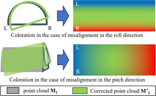
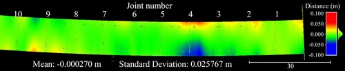
Since the measurements were taken on the same day, the higher the precision of the localization, the more consistent the tunnel shape will be. Therefore, the M3C2 distance function of Cloud Compare was used to compare and visualize the z-axis distances of the point cloud M₁ and the corrected point cloud M’₂. As shown in Figure 17, when the corresponding points are compared, the corrected point cloud M’₂ is displayed in red if it is higher and in blue if it is lower.

Figure 17. Difference in colouration due to shape difference.

Figures 18–22 show the comparison results. The uncorrected point cloud M₂ in Figure 18 shows a larger deviation than the point cloud M’₂ after the application of this method. The correction using the g-h filter shown in Figure 19 achieves a precision of less than ±5 cm, but stripe-like distortions can be seen. The corrections using the PF, EKF, and UKF shown in Figures 20–22 provide precision within ±5 cm of the distribution, but the same tendency of offset is observed on the left side of the direction of travel near joint 4. As mentioned earlier, both the point cloud M₁ and M₂ were measured on the same day, so no shape change can occur. Since there is little difference observed in the filtering results, it is believed that the distortion is due to a slight misalignment in the ICP registration.

Figure 18. Uncorrected point cloud comparison.

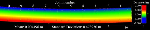
Figure 19. Corrected point cloud comparison (g-h Filter).

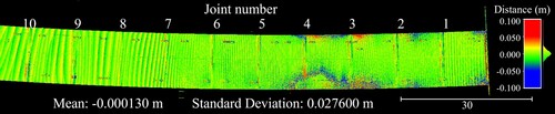
Figure 20. Corrected point cloud comparison (Particle Filter).

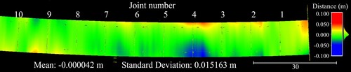
Figure 21. Corrected point cloud comparison (Extended Kalman Filter).

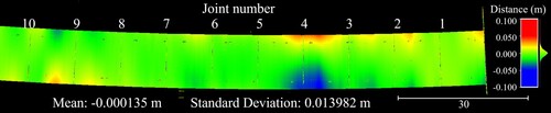
Figure 22. Corrected point cloud comparison (Unscented Kalman Filter).

5. Conclusion

In tunnels, where GNSS is not available and the environment has few features, precise localization using GNSS/IMU positioning systems or conventional scan matching is difficult due to cumulative errors. As a result, point clouds measured by MMS are distorted in shape, and correcting this distortion is costly and time-consuming.

In this work, a new method using joints in tunnels as features is proposed to improve the precision of localization in the second and subsequent differential analyses of tunnel inspections. In this method, localization was estimated by scan matching using joints as landmarks, and the point cloud data was corrected based on the estimated results. This is a method that does not diminish the advantages of mobile surveying technology, as it does not require additional surveying or traffic regulation. In addition, several types of Bayesian filters were used in this work for comparison. In all cases, the cumulative error observed before correction was corrected to less than the required precision of 0.05 m. This is expected to make it easier to compare the changes in cracks and other deformations over time in images and other media.

On the other hand, the external force nature required for the analysis of crack initiation factors is determined by comparing the 3D shapes of two different time periods, but the local distortion in the corrected point clouds makes it difficult to use them as they are. The fact that there is no significant difference in the results using each filter suggests that this local distortion is due to misalignment of the ICP registration used for sensor calibration and scan matching. Therefore, it is necessary to further reduce the registration error and to consider methods that do not cause local distortion in the future. The usefulness of the proposed registration method for determining the progression of cracks and other defects should be further validated by collecting inspection data periodically over a longer period of time.

Disclosure statement

No potential conflict of interest was reported by the author(s).

Additional information

Funding

This work was supported by the Research Committee on Technological Development for Infrastructure.

Notes on contributors

Kiichiro Ishikawa

Kiichiro Ishikawa received his B.E., M.E., and Ph.D. degrees from Waseda University in 2004, 2006, and 2010, respectively. He has been a research associate at Waseda University from 2010 to 2012, Assistant Professor at Waseda University from 2012 to 2013, Assistant Professor at Nippon Institute of Technology from 2013 to 2016; and from 2019, he has been serving as an Associate Professor. His research interests include 3D mobility measurement system and outdoor autonomous mobility systems. He is a member of The Japan Society of Mechanical Engineers, The Japan Society for Precision Engineering and The Society of Instrument and Control Engineers.

Taiga Odaka

Taiga Odaka received his B.E. degree in Mechanical Engineering from Nippon Institute of Technology, Japan in 2023. He is currently a Master course student at Nippon Institute of Technology. His research interests include localization and point cloud processing. He is a member of the Society of Instrument and Control Engineers.

References

- Ishikawa K, Takiguchi J, Amano Y, et al. Tunnel cross-section measurement system using a mobile mapping system. J Robot Mechatron. 2009;21(2):193–199. doi:10.20965/jrm.2009.p0193
- Satou A, Esaki R, Amano Y, et al. Tunnel location estimation for periodic tunnel inspections. In: JSME Conference on Robotics and mechatronics. 2020. Kanazawa (Japan): 2020. p. 1P2–L09.
- Odaka T, Ishikawa K. Localization in tunnels using feature-based scan matching. In: SICE Annual Conference September 6–9, 2023. Tsu (Japan): Mie University; 2023. p. 1284–1289.
- Sakuma Y, Ishikawa K, Yamazaki T, et al. Evaluation of a positioning correction method in GPS blockage condition. In: SICE Annual Conference September 13–18, 2011. Tokyo (Japan): Waseda University; 2011. p. 1670–1674.
- Zafari F, Gkelias A, Leung KK. A survey of indoor localization systems and technologies. IEEE Commun Surv Tutorials. 2019;21(3):2568–2599. doi:10.1109/COMST.2019.2911558
- Gan X, Yu B, Wang X, et al. A new array pseudolites technology for high precision indoor positioning. IEEE Access. 2019;7:153269–153277. doi:10.1109/ACCESS.2019.2948034
- Sun W, Xue M, Yu H, et al. Augmentation of fingerprints for indoor WiFi localization based on Gaussian process regression. IEEE Trans Veh Technol. 2018;67(11):10896–10905. doi:10.1109/TVT.2018.2870160
- Jang B, Kim H. Indoor positioning technologies without offline fingerprinting map: a survey. IEEE Commun Surv Tutorials. 2019;21(1):508–525. doi:10.1109/COMST.2018.2867935
- Mur-Artal R, Tardós JD. ORB-SLAM2: an open-source SLAM system for monocular, stereo, and RGB-D cameras. IEEE Trans Robot. 2017;33(5):1255–1262. doi:10.1109/TRO.2017.2705103
- Merzlyakov A, Macenski S. A comparison of modern general-purpose visual SLAM approaches. 2021 IEEE/RSJ International Conference on Intelligent Robots and Systems (IROS), Prague, Czech Republic; 2021. p. 9190–9197.
- Shan T, Englot B. LeGO-LOAM: lightweight and ground-optimized LiDAR odometry and mapping on variable terrain. 2018 IEEE/RSJ International Conference on Intelligent Robots and Systems (IROS), Madrid, Spain; 2018. p. 4758–4765.
- Shan T, Englot B, Meyers D, et al. LIO-SAM: tightly-coupled LiDAR inertial odometry via smoothing and mapping. 2020 IEEE/RSJ International Conference on Intelligent Robots and Systems (IROS), Las Vegas, NV, USA; 2020. p. 5135–5142.
- Chan TH, Hesse H, Ho SG. LiDAR-based 3D SLAM for indoor mapping. 2021 7th International Conference on Control, Automation and Robotics (ICCAR), Singapore; 2021. p. 285–289.
- Wang L, Zhu Y, Liu H, et al. Research on mobile robot localization and mapping method for underground long-narrow tunnels. 2022 4th International Conference on Robotics and Computer Vision (ICRCV), Wuhan, China; 2022. p. 345–349.
- Besl PJ, McKay ND. A method for registration of 3-D shapes. IEEE Trans Pattern Anal Mach Intell. 1992;14(2):239–256. doi:10.1109/34.121791
- Biber P, Strasser W. The normal distributions transform: a new approach to laser scan matching. Proceedings 2003 IEEE/RSJ International Conference on Intelligent Robots and Systems (IROS 2003) (Cat. No.03CH37453), Las Vegas, NV, USA; 2003. Vol. 3. p. 2743–2748.
- Brookner E. Tracking and Kalman filtering made easy. 1st ed., Vol. 4. New York: Wiley-Interscience; 1998.
- Thrun S, Burgard W, Fox D. Probabilistic robotics. Cambridge (MA): Massachusetts Institute of Technology; 2006.
- Kitagawa G. A Monte Carlo filtering and smoothing method for non-Gaussian nonlinear state space models. Proceedings of the 2nd U.S.-Japan Joint Seminar on Statistical Time Series Analysis Honolulu, Hawaii, January 25–29; 1993.
- Doucet A. On sequential simulation-based methods for Bayesian filtering, Technical report CUED/F-INFENG/TR.310. 1998.
- Kalman RE. A new approach to linear filtering and prediction problems. J Basic Eng. 1960;82:35–45. doi:10.1115/1.3662552
- Julier SJ, Uhlmann JK. Unscented filtering and nonlinear estimation. Proc IEEE. 2004;92(3):401–422. doi:10.1109/JPROC.2003.823141
- Jinno I, Sasaki Y, Mizoguchi H. 3D map update in human environment using change detection from LiDAR equipped mobile robot. 2019 IEEE/SICE International Symposium on System Integration (SII), Paris, France; 2019. p. 330–335.
- Chang Y-C, Chen Y-L, Hsu Y-W, et al. Integrating V-SLAM and LiDAR-based SLAM for map updating. 2021 IEEE 4th International Conference on Knowledge Innovation and Invention (ICKII), Taichung, Taiwan; 2021. p. 134–139.
- Chiang K-W, Tsai G-J, Li Y-H, et al. Development of LiDAR-based UAV system for environment reconstruction. IEEE Geosci Remote Sens Lett. 2017;14(10):1790–1794. doi:10.1109/LGRS.2017.2736013
- Tang Y, Hu Y, Cui J, et al. Vision-aided multi-UAV autonomous flocking in GPS-denied environment. IEEE Trans Ind Electron. 2019;66(1):616–626. doi:10.1109/TIE.2018.2824766
- Kim K, Im J, Jee G. Tunnel facility based vehicle localization in highway tunnel using 3D LiDAR. IEEE Trans Intell Transp Syst. 2022;23(10):17575–17583. doi:10.1109/TITS.2022.3160235
- Mengtong L, Linwei T. Synchronization technology and system based on 1 pulse per second signal. 2021 IEEE International Conference on Signal Processing, Communications and Computing (ICSPCC), Xi'an, China; 2021, p. 1–5.