Safe cooperative control of CAVs at signal-free intersection under realistic scenarios

ABSTRACT

This research deals with the cooperative control of CAVs (Connected and Automated Vehicles) at signal-free intersection. CAVs communicate with each other and adjust their speeds to safely pass through the intersection without having to stop. This is expected to improve intersection throughput and reduce fuel consumption. In order to execute cooperative control, a two-stage control structure is considered. In the first stage, the merging time, defined for each CAV as the time at which the CAV reaches the intersection, is obtained by solving mixed integer linear programming (MILP). In the second stage, each CAV solves an optimal control problem to determine the control input that allows it to reach the intersection at the merging time obtained in the first stage. In this research, a nonlinear model that considers air resistance, rolling resistance, and slope resistance is used to take into account the real environment. We propose a method using a control barrier function to guarantee the safety of CAVs even with nonlinear models , and an input correction method using a disturbance observer to suppress modelling errors caused by complex dynamics. We also propose a method that consists of establishing a speed regulation zone to avoid the possibility of passing through an intersection at an unsafe speed to improve throughput. Finally, a comparison with previous studies shows the superiority of the proposed method in reducing fuel consumption.

KEYWORDS:

• Control barrier function
• optimal control
• signal-free intersection
• mixed integer programming problem
• CAV

1. Introduction

Traffic management at intersections is important in terms of accidents and congestion on public roads. 2,583 traffic fatalities occurred in Japan in 2021, 46.6 $\mathrm{\%}$ of which were intersection-related [1]. The main cause of these fatalities is human error. As for traffic congestion, the annual traffic loss time per person is about 40 hours, which is equivalent to 40$\mathrm{\%}$ of the approximately 100 hours of riding time spent in traffic congestion [2]. Currently, traffic signals are the main cause of accidents and congestion at intersections, and there are many problems to be solved.

CASE has been attracting attention in recent years for such intersection management. CASE stands for Connected, Autonomous, Shared, Service, and Electric. Among these systems, CAVs (Connected and Automated Vehicles) are expected to be put into practical use. CAVs can communicate with each other and with the infrastructure to adjust the timing of crossing at intersections and are expected to make intersections unsignalized. Signal-free intersection is expected to reduce traffic congestion and improve throughput by reducing unnecessary stops, which CAVs are likely to reduce traffic accidents by reducing human error.

In general, control at signal-free intersections can be divided into two types [3]: centralized [4] and decentralized [5]. In the centralized type, a computing device with communication functions is installed at the centre of the intersection, and each vehicle passes through the intersection while communicating individually with this device. This method increases the computational load because the information is computed in a single location. In decentralized method, Vehicles communicate with each other in order to path through the intersection hence there still be no central device in such a method. This method is expected to reduce the computational load, but it requires vehicles unit high performance and may cause deadlock.

In general, control at unsignalized intersections is a two-stage problem, with the first stage determining the order and timing at which the vehicles cross the intersection, and the second stage determining the control inputs for the vehicle to respect their order and timing. For the first stage, FIFO (First In First Out) is often used to determine the order of crossing intersections from the viewpoint of fairness [6, 7], but from the viewpoint of efficiency, mixed integer linear programming (MILP) is used to determine the crossing schedule [8]. There are also methods that use game theory [9] and heuristic methods [10, 11]. For the second step, optimal control [12] and model predictive control (MPC) [13, 14] are used to determine the control inputs.

To reduce computational load, a method grouping several vehicles into a platoon and considering them as a single group has been proposed [15]. There is also a method using deep reinforcement learning for intersections with different shapes [16], and research focusing on ride comfort [17]. In addition, there have been many studies on safety, and many studies using control barrier functions have recently been proposed [18, 19]. Control barrier functions have attracted attention because they can determine control inputs without increasing the computational load, even for complex dynamics. Therefore, they can maintain safety even in nonlinear systems where air resistance is introduced. Safety at signal-free intersections is particularly important, but previous studies have not set a terminal speed at which vehicles pass through intersections, so safety may not be guaranteed, such as passing through an intersection at high speed. In addition, no studies have considered more specific environments, such as road surface conditions.

Based on the above studies, this study proposes a more realistic cooperative control method for CAVs at signal-free intersections that can consider air resistance and road surface conditions by using control barrier functions and disturbance observers. In addition, a speed regulation zone is established to allow the vehicle to cross the intersection at a defined terminal speed. The proposed method also allows vehicles to safely cross the intersection by avoiding crossing at unrealistic speeds due to the emphasis on efficiency.

This paper is a revised version of Ref. [20] presented at SICE Annual Conference 2023. In Chapter 3, a more detailed description of the formulated MILP optimization problem is added. Chapter 4, which describes the optimal control problem, contains the algorithm along with the formulation. Chapter 5 compares the proposed method with simulations of simple situations and conventional methods, but more complex scenarios are also examined to demonstrate the superiority of the proposed method. The computation time is also evaluated, showing that the proposed system can be operated in real-time.

2. Problem formulation

2.1. Intersection model

Consider the single-lane intersection model shown in Figure 1.

Figure 1. Intersection Model.

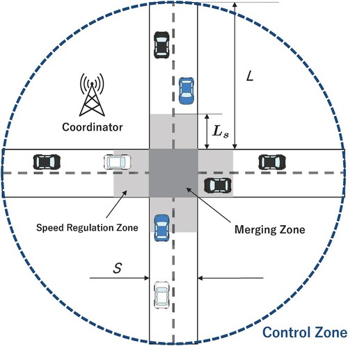
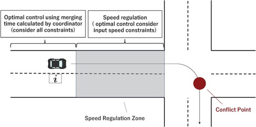
The intersection model defines three regions, the first of which is the Control Zone (CZ) delimited by a blue circle. In the CZ, it is assumed that there is a coordinator that communicates with the CAV. In the CZ, the coordinator and the CAV can communicate with each other. The second area is the Speed Regulation Zone (SRZ), a light grey area where each CAV automatically decelerates and passes through an intersection at a predetermined terminal speed. The third area is the dark grey Merging Zone (MZ), which encompasses the intersection area where conflicts may arise between CAVs in different lanes

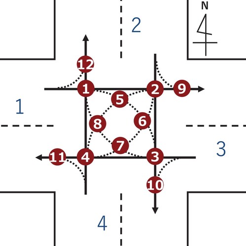
In the MZ, Conflict Point (CP) is set up as shown in the following Figure 2. CP refers to the point at which CAV${}_i$ is likely to conflict with CAV${}_j$ entering the MZ from another lane when crossing the MZ. Also, let the lanes be denoted by lane1∼4, respectively.

Figure 2. Conflict Point.

2.2. Vehicle model

The vehicle model used in this study is considered to be a model with a torque τ as shown in Figure 3.

Figure 3. Vehicle Model.

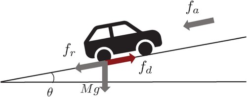
The equation of motion is (1) $M\dot{v}\left(t\right)=f_d\left(t\right)-f_a\left(t\right)-f_r\left(t\right)-f_g\left(t\right)$(1) where (2) $\begin{array}{rl}{f}_d\left(t\right)& =\frac{\tau \left(t\right)}{R_w},f_a\left(t\right)=\frac{1}{2}\rho A_f{C}_d{v}^2\left(t\right)\\ f_r\left(t\right)& =\mathrm{\mu Mgcos}\theta ,f_g\left(t\right)=\mathrm{Mgsin}\theta \end{array}$(2) where $f_d$ is the driving force of the vehicle, $f_a$ is air resistance, $f_r$ is rolling resistance, and $f_g$ is slope resistance. M is the vehicle weight and $R_w$ is the tire radius. Explanations for each letter are given in Table 1. The vehicle is equipped with automatic driving and communication functions to perform cooperative control alongside multiple vehicles. From the equations of motion, we have $\frac{1}{2}\rho A_f{C}_d{v}_i^2\left(t\right)+\mathrm{\mu Mgcos}\theta +\mathrm{Mgsin}\theta =F\left(v_i\right(t\left)\right)$. Hence we can represent the state space model of some CAV${}_i$ as (3) $\left[\begin{array}{c}{\dot{p}}_i\left(t\right)\\ {\dot{v}}_i\left(t\right)\end{array}\right]=\left[\begin{array}{c}{v}_i\left(t\right)\\ -\frac{F\left(v_i\right(t\left)\right)}{M}\end{array}\right]+\left[\begin{array}{c}0\\ \frac{1}{M{R}_w}\end{array}\right]{\tau }_i\left(t\right)$(3) where $p_i$ is the position of CAV${}_i$ and $v_i$ is the speed of CAV${}_i$. In addition, from the viewpoint of vehicle performance and passenger comfort, input and speed constraints are set as shown in (4(4) $\begin{array}{rl}{\tau }_{min}& \le {\tau }_i\left(t\right)\le {\tau }_{max}\\ v_{min}& \le v_i\left(t\right)\le v_{max}\end{array}$(4) ). (4) $\begin{array}{rl}{\tau }_{min}& \le {\tau }_i\left(t\right)\le {\tau }_{max}\\ v_{min}& \le v_i\left(t\right)\le v_{max}\end{array}$(4) Let us assume that the following assumptions hold for CAV.

Assumption 2.1

At a signal-free intersection, only CAVs of at least Level 4 shall be present, with no communication problems such as errors or delays, pedestrians, and all CAVs shall have the same width and length, mass, and equipment.

Table 1. Symbol.

Symbols	Definition
M	Weight of vehicle [kg]
$R_w$	Tire radius [m]
ρ	Air density [$\mathrm{kg}/{\mathrm{m}}^3$]
$C_d$	Air resistance coefficient
$A_f$	Vehicle frontal area [${\mathrm{m}}^2$]
μ	Rolling resistance coefficient
θ	Road tilt angle [rad]

2.3. Control structure

In this study, we consider an optimization control structure divided into two levels: the coordinator level and the CAV level. In the coordinator-level optimization, the optimal merging time is calculated based on the information from each CAV, so that no conflicts occur between CAVs from the time they enter the SRZ to the time they exit the MZ. The merging time represents the duration for CAVs to reach the SRZ, and the calculation is performed either at a specified time step or when a new CAV enters the CZ. Coordinator-level optimization is a static optimization problem, and CAV-level optimization is a dynamic optimization problem. In terms of the perspective of computational load, we consider a control structure that is divided into two as shown in Figure 4.

Figure 4. Control Structure.

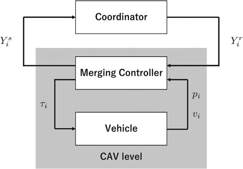
where $Y_i^s\triangleq \{{\eta }_i,p_i,v_i,t_{i,\mathrm{prev}}^m\}$ is the dataset sent from CAV${}_i$ to Coordinator, $Y_i^r\triangleq \{{t^m}_i^{\ast },p_i({t^m}_i^{\ast })$,$v_i\left({t_i^m}^{\ast }\right)\}$ is the dataset sent from Coordinator to CAV${}_i$. Also, ${\eta }_i$ is the travel lane, ${t_i^m}^{\ast }$ is the optimal merging time calculated by the Coordinator and $t_{i,\mathrm{prev}}^m$ is the merging time calculated by the Coordinator at the previous sampling time.

2.4. Speed regulation zone

SRZ performs deceleration using a predetermined speed regulation time $t_i^{\mathrm{sr}}$ as shown in Figure 5.

Figure 5. Speed Regulation Zone.

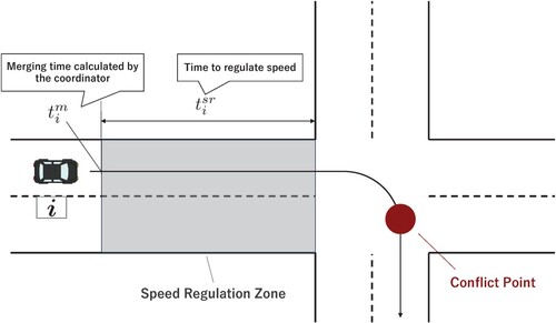
The speed is reduced to a predetermined terminal speed using the speed regulation time $t_i^{\mathrm{sr}}$ and the right/left turn and straight ahead information of each CAV. If the terminal speed is not fixed, drivers may turn right or left at higher speed to improve throughput, which may cause comfort and safety problems. Since this study uses a two-stage control structure, fixing the terminal speed at the Coordinator-level optimization has the advantage that it is easier to find a collision-free merging time.

3. Coordinator-level optimization

This chapter shows how Coordinator determines the optimal merging time for each CAV, which is the optimal time at which each CAV crosses the intersection to avoid conflicts with other CAVs and increase the throughput at the intersection.

3.1. Objective function

The objective of the coordinator-level optimization is to make the CAV pass through the intersection as safely and as quickly as possible. Therefore, the objective function is set as follows. (5) $\underset{T}{\min }\sum _{i=1}^{N\left(t\right)}{t}_i^m$(5) where $N\left(t\right)$ is the number of CAVs in the CZ and T is the decision variable $T=[{t_1^m}^{\ast },{t_2^m}^{\ast },\dots ,t_{N\left(t\right)}^{m\ast }]$ for the optimization problem.

3.2. Constraints

First, We consider the lower boundary of the merging time. This boundary is related to CAVs performance. For this reason, the following constraint equation is used (6) $t_i^m\ge t_{i,min}^m$(6) This is the time it takes for the CAV to reach the SRZ at its fastest speed from its current position. CAV accelerates at the maximum input and travels at a constant speed once it reaches the maximum speed. When the CAV enters SRZ, it decelerates with the minimum input because the terminal speed is fixed as in the MZ. Depending on the current position and speed, the maximum speed may not be reached, the minimum merging time can be classified into two patterns as shown in Figures 6 and 7.

Figure 6. Minimum merging time pattern (a).

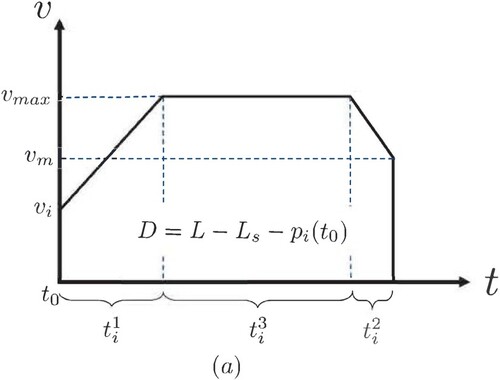
Figure 7. Minimum merging time pattern (b).

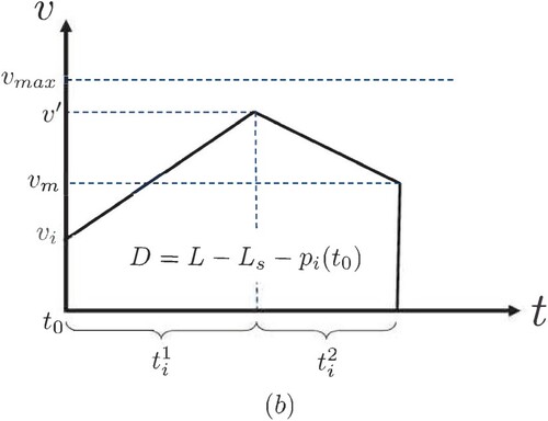
where $D=L-L_s-p_i\left(t\right)$ in Figures 6 and 7 is the distance from the current distance to the SRZ. Pattern (a) is the case where the vehicle accelerates at maximum acceleration and reaches maximum speed. Conversely, Pattern (b) is the case where the vehicle accelerates at the maximum acceleration but does not reach the maximum speed. The specific values for each pattern are as follows. (7) $\begin{array}{rl}{t}_{i,min}^m& =\frac{M{R}_w(v_{max}-v_i)}{{\tau }_{max}}+\frac{M{R}_w(v_m-v_{max})}{{\tau }_{min}}\\ & +\frac{D-\frac{M{R}_w(v_{max}^2-v_i^2)}{2{\tau }_{max}}-\frac{M{R}_w(v_m^2-v_{max}^2)}{2{\tau }_{min}}}{v_{max}}\dots \left(a\right)\\ t_{i,min}^m& =\frac{M{R}_w(v^{\prime }-v_i)}{{\tau }_{max}}+\frac{M{R}_w(v_m-v^{\prime })}{{\tau }_{min}}\dots \left(b\right)\\ & \mathrm{where}{v}^{\prime }=\sqrt{\frac{\frac{2D}{M{R}_w}+\frac{{v_i}^2}{{\tau }_{max}}-\frac{{v_m}^2}{{\tau }_{min}}}{\frac{1}{{\tau }_{max}}-\frac{1}{{\tau }_{min}}}}\end{array}$(7) (a) is the case where the maximum speed in Equation (4(4) $\begin{array}{rl}{\tau }_{min}& \le {\tau }_i\left(t\right)\le {\tau }_{max}\\ v_{min}& \le v_i\left(t\right)\le v_{max}\end{array}$(4) ) is reached between the current position and the entrance to the SRZ. When the maximum speed is reached, the vehicle cannot accelerate anymore, so it runs at a constant speed and then decelerates so that it can eventually enter the SRZ at the terminal speed. (b) is the case where the maximum speed is not reached. In this case, the vehicle does not travel at a constant speed, but accelerates at maximum torque and decelerates at minimum torque to enter the SRZ at the terminal speed.

Next, constraints are set to avoid a rear-end conflict with a preceding vehicle (CAV${}_k$) in the same lane. Rear-end conflict constraints are as (8) $t_i^m-t_k^m\ge \frac{{\alpha }_i\left(t\right)}{v_{m,k}}=h_R,{\eta }_k={\eta }_i$(8) where ${\alpha }_i\left(t\right)=\delta +l_k+\phi v_i\left(t\right)$ and δ is the safety distance between the CAV${}_k$ rear bumper and the CAV${}_i$ front bumper, φ is the reaction time of CAV${}_i$, and $l_k$ is the length of the CAV${}_k$. η is a lane of CAVs. With this constraint, rear-end conflict can be avoided in the MZ. In order to avoid rear-end conflict in the SRZ, a speed regulation time $t_i^{\mathrm{sr}}$ is added to the Equation (8(8) $t_i^m-t_k^m\ge \frac{{\alpha }_i\left(t\right)}{v_{m,k}}=h_R,{\eta }_k={\eta }_i$(8) ). The equation for the rear-end conflict constraint is (9) $(t_i^m+t_i^{\mathrm{sr}})-(t_k^m+t_k^{\mathrm{sr}})\ge h_R$(9) The rear-end conflict constraints shown here are intended to avoid conflicts from entering the SRZ until passing through the MZ. In other words, rear-end conflict before entering the SRZ is not considered. Therefore, CAVs must communicate with each other to avoid collisions until they enter the SRZ.

Next, consider a constraint to avoid a lateral conflict with a CAV running in a different lane. The likelihood of a conflict is determined from Figure 2. As shown in Figure 8, the Conflict Zone is a circle with a radius of r centred at the CP. The time taken by the CAV${}_i$ to enter the Conflict Zone after entering the MZ is $t_i^e$, the time taken by the CAV${}_i$ to exit the Conflict Zone after entering the MZ is $t_i^l$.

Figure 8. Lateral Headway Time.

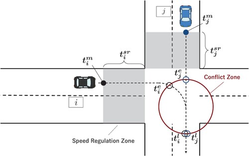
Using these to consider the lateral conflict constraints, we consider the speed regulation time $t_i^{\mathrm{sr}}$ as well as the rear-end conflict constraints, and we obtain (10) $\begin{array}{r}\begin{array}{rl}& (t_i^m+t_i^e+t_i^{\mathrm{sr}})+M_{\mathrm{big}}{b}_{\mathrm{ij}}\ge (t_j^m+t_j^l+t_j^{\mathrm{sr}})+h_L\\ & \mathrm{AND}\\ & (t_j^m+t_j^e+t_j^{\mathrm{sr}})+M_{\mathrm{big}}(1-b_{\mathrm{ij}})\ge (t_i^m+t_i^l+t_i^{\mathrm{sr}})+h_L\end{array}\end{array}$(10) where $h_L$ represents the time required for the CAV to completely exit the Conflict Zone. In this case, the position of the CAV is the front bumper, so consider the time it takes for the rear bumper of the CAV to completely exit the conflict zone. In addition, if the equation is expressed with OR, it becomes discontinuous, so it is expressed with an AND equation using the Big-M method [21], where $b_{\mathrm{ij}}$ is a binary variable.

The Coordinator performs calculations at each defined time step or when a new CAV enters the CZ. In such cases, there may be a large difference between the previously calculated merging time and the newly calculated merging time. In such a case, the CAV may need to perform a sudden acceleration/deceleration. However sudden changes in acceleration should be minimized to ensure comfort, safety, and fuel efficiency. For this reason, an objective function is added as follows. (11) $\underset{T,T^{\mathrm{abs}}}{\min }w\sum _{i=1}^{N\left(t\right)}{t}_i^m+(1-w)\sum _{i=1}^{N\left(t\right)}{t}_i^{\mathrm{abs}}$(11) where $t_i^{\mathrm{abs}}=|t_i^m-t_{i,\mathrm{prev}}^m|$ and w is the weight. From the above, we add to the constraint the following ones. (12) $\begin{array}{rl}{t}_i^{\mathrm{abs}}& \ge (t_i^m-t_{i,\mathrm{prev}}^m)\end{array}$(12) (13) $\begin{array}{rl}{t}_i^{\mathrm{abs}}& \ge -(t_i^m-t_{i,\mathrm{prev}}^m)\end{array}$(13) In summary, the optimal merging times calculated by the Coordinator can be obtained by solving (14) $\begin{array}{rl}\underset{T,B,T^{\mathrm{abs}}}{\min }& w\sum _{i=1}^{N\left(t\right)}{t}_i^m+(1-w)\sum _{i=1}^{N\left(t\right)}{t}_i^{\mathrm{abs}}\\ & T\in {\mathbb{R}}^{N\left(t\right)},T^{\mathrm{abs}}\in {\mathbb{R}}^{N\left(t\right)}\\ & B\in \{0,1{\}}^{K\left(t\right)},K(t)\le \frac{N^2\left(t\right)-N\left(t\right)}{2}\\ \mathrm{subject}\mathrm{to}:& t_i^m\ge t_{i,min}^m\\ & (t_i^m+t_i^{\mathrm{sr}})-(t_k^m+t_k^{\mathrm{sr}})\ge h_R{\eta }_i={\eta }_k\\ & (t_i^m+t_i^e+t_i^{\mathrm{sr}})+M_{\mathrm{big}}{b}_{\mathrm{ij}}\\ & \ge (t_j^m+t_j^l+t_j^{\mathrm{sr}})+h_L\\ & (t_j^m+t_j^e+t_j^{\mathrm{sr}})+M_{\mathrm{big}}(1-b_{\mathrm{ij}})\\ & \ge (t_i^m+t_i^l+t_i^{\mathrm{sr}})+h_L\\ & t_i^{\mathrm{abs}}\ge (t_i^m-t_{i,\mathrm{prev}}^m)\\ & t_i^{\mathrm{abs}}\ge -(t_i^m-t_{i,\mathrm{prev}}^m),\end{array}$(14) $T_i^{\mathrm{abs}}$, $N\left(t\right)$ is the set of $T_i^{\mathrm{abs}}$ and the total number of CAVs in the CZ, respectively. Also, B is a set of binary variables $b_{\mathrm{ij}}$ to determine the order in which CAV${}_i$ and CAV${}_j$ intersect.

The difference between the merging time $t_i^m$ and the previous merging time $t_i^{\mathrm{abs}}$ is a real number, while the binary variable $b_{\mathrm{ij}}$ takes on integer values of 0 or 1. Optimization problems in which the decision variables are a mixture of real numbers and integers are called mixed integer linear programming (MILP).

Finally the algorithm is given below.

4. CAV-level optimization

In this section, we formulate the problem of determining the control input for the CAV by solving the optimal control problem based on the optimal merging time calculated by the Coordinator. In addition to speed and input constraints, a cooperative control framework is presented to allow the CAV to pass through an intersection without conflict with other CAVs.

4.1. Formulation of the optimal control problem

The optimal control problem solved by each CAV is as follows. (15) $\begin{array}{r}\begin{array}{rl}\underset{{\tau }_i\left(t\right)}{\min }& {\displaystyle {\int }_{t_i^0}^{t_i^m}\frac{1}{2}{\tau }_i^2\left(t\right)\mathrm{d}t}\\ \mathrm{subject}\mathrm{to}:& \mathrm{CAV}\mathrm{model}\left(3\right)\\ & {\tau }_{min}\le {\tau }_i\left(t\right)\le {\tau }_{max}\\ & v_{min}\le v_i\left(t\right)\le v_{max}\\ & p_k\left(t\right)-p_i\left(t\right)\ge \phi v_i\left(t\right)+\delta \\ & \mathrm{given}{p}_i\left(t_i^0\right),v_i\left(t_i^0\right),v_i\left(t_i^m\right),p_i\left(t_i^m\right)\end{array}\end{array}$(15) The constraints are an input constraint, a speed constraint, and a rear-end conflict constraint to prevent conflict before entering SRZ. The $t_i^0$ is the current time.

Our goal is to find an analytical solution to the optimal control problem. However, this task is complicated due to the presence of $v_i$ in the resistance term, like air resistance in (15(15) $\begin{array}{r}\begin{array}{rl}\underset{{\tau }_i\left(t\right)}{\min }& {\displaystyle {\int }_{t_i^0}^{t_i^m}\frac{1}{2}{\tau }_i^2\left(t\right)\mathrm{d}t}\\ \mathrm{subject}\mathrm{to}:& \mathrm{CAV}\mathrm{model}\left(3\right)\\ & {\tau }_{min}\le {\tau }_i\left(t\right)\le {\tau }_{max}\\ & v_{min}\le v_i\left(t\right)\le v_{max}\\ & p_k\left(t\right)-p_i\left(t\right)\ge \phi v_i\left(t\right)+\delta \\ & \mathrm{given}{p}_i\left(t_i^0\right),v_i\left(t_i^0\right),v_i\left(t_i^m\right),p_i\left(t_i^m\right)\end{array}\end{array}$(15) ). To overcome this complexity, we first obtain an analytical solution in an ideal scenario where there is no resistance. The analytical solution is as follows. (16) $\begin{array}{rl}{\tau }_i^{\ast }& =C_{1}t+C_2\\ v_i^{\ast }& =\frac{1}{M{R}_w}(\frac{1}{2}{C}_1{t}^2+C_{2}t+C_3)\\ p_i^{\ast }& =\frac{1}{M{R}_w}(\frac{1}{6}{C}_1{t}^3+\frac{1}{2}{C}_2{t}^2+C_{3}t+C_4)\end{array}$(16) where $C_1,C_2,C_3,C_4$ are integration constants that can be obtained using the boundary conditions $p_i\left(t_i^0\right),v_i\left(t_i^0\right),v_i\left(t_i^m\right),p_i\left(t_i^m\right)$.

4.2. Input correction

In the real environment, even if the analytical solution is used, the speed and position will deviate from the trajectory when there is a resistance such as (2(2) $\begin{array}{rl}{f}_d\left(t\right)& =\frac{\tau \left(t\right)}{R_w},f_a\left(t\right)=\frac{1}{2}\rho A_f{C}_d{v}^2\left(t\right)\\ f_r\left(t\right)& =\mathrm{\mu Mgcos}\theta ,f_g\left(t\right)=\mathrm{Mgsin}\theta \end{array}$(2) ). Therefore, in order to eliminate modelling errors, we consider a method to correct the input using a disturbance observer such as the following. (17) ${\tau }_i^{\mathrm{ref}}\left(t\right)={\tau }_i^{\ast }\left(t\right)+\widehat{d_i}\cdot R_w$(17) where $\widehat{d_i}$ is the estimated resistance $F\left(v_i\right(t\left)\right)$. The purpose of this disturbance observer is to estimate the resistance $F\left(v_i\right(t\left)\right)$, and add it to the input to cancel resistance out and track the trajectory. Using ${\tau }_i^{\mathrm{ref}}$ obtained from the input correction, CAV solves the optimal control problem.

4.3. Formulation with control barrier function

In the constraints outlined in Equation (15(15) $\begin{array}{r}\begin{array}{rl}\underset{{\tau }_i\left(t\right)}{\min }& {\displaystyle {\int }_{t_i^0}^{t_i^m}\frac{1}{2}{\tau }_i^2\left(t\right)\mathrm{d}t}\\ \mathrm{subject}\mathrm{to}:& \mathrm{CAV}\mathrm{model}\left(3\right)\\ & {\tau }_{min}\le {\tau }_i\left(t\right)\le {\tau }_{max}\\ & v_{min}\le v_i\left(t\right)\le v_{max}\\ & p_k\left(t\right)-p_i\left(t\right)\ge \phi v_i\left(t\right)+\delta \\ & \mathrm{given}{p}_i\left(t_i^0\right),v_i\left(t_i^0\right),v_i\left(t_i^m\right),p_i\left(t_i^m\right)\end{array}\end{array}$(15) ), the input variable ${\tau }_i$ is not explicitly incorporated into the constraint equation. As a result, when constraints become active, it is difficult to determine inputs based on these constraints. To address this issue, we adopt a formulation involving a control barrier function. For simplicity, we consider the vehicle model as depicted in (18(18) $\dot{x}=f\left(x\right)+g\left(x\right)u$(18) ). (18) $\dot{x}=f\left(x\right)+g\left(x\right)u$(18) Then define the control barrier function. First, we define the safe set.

Definition 4.1

safe set of CAV${}_i$

Consider a $C^1$ class function $h:X\to \mathbb{R}$ and a set $\mathcal{C}\subset X$ expressed as follows. (19) $\begin{array}{rl}\mathcal{C}& =\{x_i\in X\mid h(x_i)\ge 0\}\\ \mathrm{\partial }\mathcal{C}& =\{x_i\in X\mid h(x_i)=0\}\\ \mathrm{Int}\left(\mathcal{C}\right)& =\{x_i\in X\mid h(x_i)>0\}\end{array}$(19) If the state $x_i$ of CAV${}_i$ satisfies $x\in \mathcal{C}$, then $\mathcal{C}$ is a safe set.

This safe set is only for CAV${}_i$. For the rear-end conflict constraint, information on the preceding vehicle, CAV${}_k$, is also required, hence a 2 CAVs safe set is also needed.

Definition 4.2

safe set of CAV${}_i$, CAV${}_k$

Consider a $C^1$ class function $H:X_i\times X_k\to \mathbb{R}$ and a safe set ${\mathcal{C}}^{\prime }\subset X_i\times X_k$ expressed as follows. (20) $\begin{array}{rl}{\mathcal{C}}^{\prime }& =\left\{\right(x_i,x_k)\in X_i\times X_k\mid H(x_i,x_k)\ge 0\}\\ \mathrm{\partial }{\mathcal{C}}^{\prime }& =\left\{\right(x_i,x_k)\in X_i\times X_k\mid H(x_i,x_k)=0\}\\ \mathrm{Int}\left({\mathcal{C}}^{\prime }\right)& =\left\{\right(x_i,x_k)\in X_i\times X_k\mid H(x_i,x_k)>0\}\end{array}$(20)

Next, we define a forward invariant set obtained from a safe set.

Definition 4.3

forward invariant set

A set $\mathcal{C}$ is said to be a forward invariant set if the initial state $x\left(0\right)$ of the system (3(3) $\left[\begin{array}{c}{\dot{p}}_i\left(t\right)\\ {\dot{v}}_i\left(t\right)\end{array}\right]=\left[\begin{array}{c}{v}_i\left(t\right)\\ -\frac{F\left(v_i\right(t\left)\right)}{M}\end{array}\right]+\left[\begin{array}{c}0\\ \frac{1}{M{R}_w}\end{array}\right]{\tau }_i\left(t\right)$(3) ) is contained in the set $\mathcal{C}$ and $x\in \mathcal{C}$ at any time $t\in [0,\mathrm{\infty })$.

This forward invariant set can likewise be defined for the safe set of 2 CAVs. Next, we define the extended class $\mathcal{K}$ function.

Definition 4.4

extended class $\mathcal{K}$ function

Consider a continuous function $\alpha :\mathbb{R}\to \mathbb{R}$. When this function is strictly monotonically increasing and satisfies $\alpha \left(0\right)=0$, it is called an extended class $\mathcal{K}$ function.

Finally, we define the control barrier function.

Definition 4.5

control barrier function

Let h be a $C^1$ function and let $\mathcal{C}\subset X$ be the safe set of CAV${}_i$ for the vehicle model (3(3) $\left[\begin{array}{c}{\dot{p}}_i\left(t\right)\\ {\dot{v}}_i\left(t\right)\end{array}\right]=\left[\begin{array}{c}{v}_i\left(t\right)\\ -\frac{F\left(v_i\right(t\left)\right)}{M}\end{array}\right]+\left[\begin{array}{c}0\\ \frac{1}{M{R}_w}\end{array}\right]{\tau }_i\left(t\right)$(3) ). If there exists an extended class $\mathcal{K}$ function α that satisfies the following inequality (21(21) $\underset{u_i\in U_i}{sup}\dot{h}\left(x_i\right)+\alpha \left(h\right(x_i\left)\right)\ge 0$(21) ), then the function h is called a control barrier function defined on $\mathcal{C}$. (21) $\underset{u_i\in U_i}{sup}\dot{h}\left(x_i\right)+\alpha \left(h\right(x_i\left)\right)\ge 0$(21)

Here, $\dot{h}\left(x_i\right)$ can be expressed as $\dot{h}\left(x_i\right)=L_{f}h\left(x_i\right)+L_{g}h\left(x_i\right)u_i$ by the Lie derivative We can define the following set $K_i\left(x_i\right)$ from this control barrier function h.

Definition 4.6

$K_i\left(x_i\right)$

(22) $K_i\left(x_i\right)=\{u_i\in U_i:\dot{h}(x_i)+\alpha (h\left(x_i\right))\ge 0\}$(22)

Definition 4.7

control barrier function

Let ${\mathcal{C}}^{\prime }$ be the safe set of CAV${}_i$ and CAV${}_k$, and let $H:X_i\times X_k\to \mathbb{R}$ be a $C^1$ function. If there exists an extended class $\mathcal{K}$ function that satisfies the following inequality for the safe set ${\mathcal{C}}^{\prime }$, H is called a control barrier function. (23) $\underset{(u_i,u_k)\in U_i\times U_k}{sup}\dot{H}(x_i,x_k)\ge -\alpha \left(H\right(x_i,x_k\left)\right)$(23)

We can define the following set $K_H\left(x\right)$ from this control barrier function H

Definition 4.8

$K_H\left(x\right)$

(24) $\begin{array}{rl}{K}_H\left(x\right)& =\left\{\right(u_i,u_k)\in U_i\times U_k:\dot{H}(x_i,x_k)\\ & \ge -\alpha \left(H\right(x_i,x_k\left)\right)\}\end{array}$(24)

A control barrier function is then defined. Using the input obtained from the control barrier function, it can be said that the input stays within the safe set, i.e. forward invariance is satisfied.

Theorem 4.1

Let $\mathcal{C}$ be a safe set of CAV${}_i$. When $h\left(x_i\right)$ is a control barrier function, the Lipschitz continuous input $u\in K_i\left(x_i\right)$ satisfies forward invariance on the safe set.

Proof.

Since $\dot{h}\left(x_i\right)$ is always greater than or equal to 0 at the boundary of the safe set, it satisfies forward invariance by Nagumo's theorem [22].

Theorem 4.2

Let ${\mathcal{C}}^{\prime }$ be the safe set of ${\mathrm{CAV}}_i$ and ${\mathrm{CAV}}_k$, and $H:X_i\times X_k\to \mathbb{R}$ be a $C^1$ class function. When H is a control barrier function, the Lipschitz continuous $(u_i,u_k)\in K_H(x_i,x_k)$ satisfies forward invariance on the safe set.

Proof.

We consider $\begin{array}{rl}z& =\left[\begin{array}{c}{x}_i\\ x_k\end{array}\right],u^{\prime }=\left[\begin{array}{c}{u}_i\\ u_k\end{array}\right],F\left(z\right)=\left[\begin{array}{c}f\left(x_i\right)\\ f\left(x_k\right)\end{array}\right],\\ G\left(z\right)& =\left[\begin{array}{c}g\left(x_i\right)\\ g\left(x_k\right)\end{array}\right]\end{array}$we can set $H(x_i,x_k)=H\left(z\right)$, which satisfies forward invariance by Nagumo's theorem as well as Theorem 4.1. [19, 23].

Therefore, it is confirmed that forward invariance is satisfied.

The candidate control barrier functions used in this study are then shown in (25(25) $\begin{array}{rl}{h}_1\left(x_i\right)& =v_i\left(t\right)-v_{min}\\ h_2\left(x_i\right)& =v_{max}-v_i\left(t\right)\\ H(x_i,x_j)& =p_k\left(t\right)-p_i\left(t\right)-\phi v_i\left(t\right)-\delta \end{array}$(25) ). (25) $\begin{array}{rl}{h}_1\left(x_i\right)& =v_i\left(t\right)-v_{min}\\ h_2\left(x_i\right)& =v_{max}-v_i\left(t\right)\\ H(x_i,x_j)& =p_k\left(t\right)-p_i\left(t\right)-\phi v_i\left(t\right)-\delta \end{array}$(25) where $h_1,h_2$ are the minimum and maximum speed constraints, respectively. Also, H is the rear-end conflict constraint.

Finally, using this control barrier function, the optimal control problem (15(15) $\begin{array}{r}\begin{array}{rl}\underset{{\tau }_i\left(t\right)}{\min }& {\displaystyle {\int }_{t_i^0}^{t_i^m}\frac{1}{2}{\tau }_i^2\left(t\right)\mathrm{d}t}\\ \mathrm{subject}\mathrm{to}:& \mathrm{CAV}\mathrm{model}\left(3\right)\\ & {\tau }_{min}\le {\tau }_i\left(t\right)\le {\tau }_{max}\\ & v_{min}\le v_i\left(t\right)\le v_{max}\\ & p_k\left(t\right)-p_i\left(t\right)\ge \phi v_i\left(t\right)+\delta \\ & \mathrm{given}{p}_i\left(t_i^0\right),v_i\left(t_i^0\right),v_i\left(t_i^m\right),p_i\left(t_i^m\right)\end{array}\end{array}$(15) ) can be rewritten (26) $\begin{array}{rl}\underset{{\tau }_i\left(t\right)}{\min }& {\displaystyle {\int }_{t_i^0}^{t_i^m}\frac{1}{2}{\left({\tau }_i^{\mathrm{ref}}\right(t)-{\tau }_i(t\left)\right)}^2\mathrm{d}t}\\ \mathrm{subject}\mathrm{to}:& \mathrm{CAV}\mathrm{model}\left(3\right)\\ & {\tau }_i\left(t\right)-{\tau }_{min}\ge 0\\ & {\tau }_{max}-{\tau }_i\left(t\right)\ge 0\\ & -\frac{F\left(v_i\right(t\left)\right)}{M}+\frac{1}{M{R}_w}{\tau }_i\left(t\right)+v_i\left(t\right)-v_{min}\\ & \ge 0\\ & \frac{F\left(v_i\right(t\left)\right)}{M}-\frac{1}{M{R}_w}{\tau }_i\left(t\right)+v_{max}-v_i\left(t\right)\\ & \ge 0\\ & v_k\left(t\right)-v_i\left(t\right)+\frac{F\left(v_i\right(t\left)\right)}{M}-\frac{\phi }{M{R}_w}{\tau }_i\left(t\right)\\ & +p_k\left(t\right)-p_i\left(t\right)-\phi v_i\left(t\right)-\delta \ge 0\\ & \mathrm{given}{p}_i\left(t_i^0\right),v_i\left(t_i^0\right),v_i\left(t_i^m\right),p_i\left(t_i^m\right)\end{array}$(26) The objective function $\left({\tau }_i^{\mathrm{ref}}\right(t)-{\tau }_i(t){)}^2$ is used to track the torque ${\tau }_i^{\mathrm{ref}}$ after input correction.

4.4. Optimal control problem in speed regulation zone

Finally, we explain optimal control in the SRZ. In SRZ, deceleration is performed using a predetermined speed regulation time $t^{\mathrm{sr}}$. Also, since conflicts within the SRZ are taken into account in the optimization at the coordinator level, unlike (26(26) $\begin{array}{rl}\underset{{\tau }_i\left(t\right)}{\min }& {\displaystyle {\int }_{t_i^0}^{t_i^m}\frac{1}{2}{\left({\tau }_i^{\mathrm{ref}}\right(t)-{\tau }_i(t\left)\right)}^2\mathrm{d}t}\\ \mathrm{subject}\mathrm{to}:& \mathrm{CAV}\mathrm{model}\left(3\right)\\ & {\tau }_i\left(t\right)-{\tau }_{min}\ge 0\\ & {\tau }_{max}-{\tau }_i\left(t\right)\ge 0\\ & -\frac{F\left(v_i\right(t\left)\right)}{M}+\frac{1}{M{R}_w}{\tau }_i\left(t\right)+v_i\left(t\right)-v_{min}\\ & \ge 0\\ & \frac{F\left(v_i\right(t\left)\right)}{M}-\frac{1}{M{R}_w}{\tau }_i\left(t\right)+v_{max}-v_i\left(t\right)\\ & \ge 0\\ & v_k\left(t\right)-v_i\left(t\right)+\frac{F\left(v_i\right(t\left)\right)}{M}-\frac{\phi }{M{R}_w}{\tau }_i\left(t\right)\\ & +p_k\left(t\right)-p_i\left(t\right)-\phi v_i\left(t\right)-\delta \ge 0\\ & \mathrm{given}{p}_i\left(t_i^0\right),v_i\left(t_i^0\right),v_i\left(t_i^m\right),p_i\left(t_i^m\right)\end{array}$(26) ), no rear-end conflict constraint is set in the optimal control problem in Figure 9. (27) $\begin{array}{rl}\underset{{\tau }_i\left(t\right)}{\min }& {\displaystyle {\int }_{t_i^m}^{t_i^m+t_i^{\mathrm{sr}}}\frac{1}{2}{\left({\tau }_i^{\mathrm{ref}}\right(t)-{\tau }_i(t\left)\right)}^2\mathrm{d}t}\\ \mathrm{subject}\mathrm{to}:& \mathrm{CAVmodel}\left(3\right)\\ & {\tau }_i\left(t\right)-{\tau }_{min}\ge 0\\ & {\tau }_{max}-{\tau }_i\left(t\right)\ge 0\\ & -\frac{F\left(v_i\right(t\left)\right)}{M}+\frac{1}{M{R}_w}{\tau }_i\left(t\right)+v_i\left(t\right)-v_{min}\\ & \ge 0\\ & \frac{F\left(v_i\right(t\left)\right)}{M}-\frac{1}{M{R}_w}{\tau }_i\left(t\right)+v_{max}-v_i\left(t\right)\ge 0\\ & \mathrm{given}{p}_i\left(t_i^m\right),v_i\left(t_i^m\right),v_i(t_i^m+t_i^{\mathrm{sr}}),\\ & p_i(t_i^m+t_i^{\mathrm{sr}})\end{array}$(27)

Figure 9. Optimal Control in SRZ.

4.5. Algorithm of optimal control

Finally, we include the algorithm for the optimal control problem solved by each CAV, which determines its inputs according to Algorithm 2 below.

5. Simulation verification

5.1. Simulation conditions

In order to verify the simulation, we set the parameters as in Table 2.

Table 2. Simulation parameter.

Parameter	Symbol	Value
Number of vehicles	$N_{max}$	50
Vehicle arrival rate(1/h)	$f^a$	720
Control Zone(m)	L	300
Speed Regulation Zone(m)	$L_s$	30
Size of Merging Zone(m)	S	10
Radius of conflict point zone(m)	r	4
Weight of optimization problem (14(14) $\begin{array}{rl}\underset{T,B,T^{\mathrm{abs}}}{\min }& w\sum _{i=1}^{N\left(t\right)}{t}_i^m+(1-w)\sum _{i=1}^{N\left(t\right)}{t}_i^{\mathrm{abs}}\\ & T\in {\mathbb{R}}^{N\left(t\right)},T^{\mathrm{abs}}\in {\mathbb{R}}^{N\left(t\right)}\\ & B\in \{0,1{\}}^{K\left(t\right)},K(t)\le \frac{N^2\left(t\right)-N\left(t\right)}{2}\\ \mathrm{subject}\mathrm{to}:& t_i^m\ge t_{i,min}^m\\ & (t_i^m+t_i^{\mathrm{sr}})-(t_k^m+t_k^{\mathrm{sr}})\ge h_R{\eta }_i={\eta }_k\\ & (t_i^m+t_i^e+t_i^{\mathrm{sr}})+M_{\mathrm{big}}{b}_{\mathrm{ij}}\\ & \ge (t_j^m+t_j^l+t_j^{\mathrm{sr}})+h_L\\ & (t_j^m+t_j^e+t_j^{\mathrm{sr}})+M_{\mathrm{big}}(1-b_{\mathrm{ij}})\\ & \ge (t_i^m+t_i^l+t_i^{\mathrm{sr}})+h_L\\ & t_i^{\mathrm{abs}}\ge (t_i^m-t_{i,\mathrm{prev}}^m)\\ & t_i^{\mathrm{abs}}\ge -(t_i^m-t_{i,\mathrm{prev}}^m),\end{array}$(14) )	w	0.3
Length of CAV(m)	$l_i$	4
Standstill safe distance(m)	δ	8
CAV reaction time(s)	φ	0.8
SpeedRegulation time(straight)(s)	$t_S^{\mathrm{sr}}$	3.0
SpeedRegulation time(right)(s)	$t_R^{\mathrm{sr}}$	3.6
SpeedRegulation time(left)(s)	$t_L^{\mathrm{sr}}$	4.5
Speed when going straight(m/s)	$v_S$	10
Speed when turning right(m/s)	$v_R$	7
Speed when turning left(m/s)	$v_L$	3
Minimum speed(m/s)	$v_{min}$	0
Maximum speed(m/s)	$v_{max}$	16
Minimum input($\mathrm{kg}{\mathrm{m}}^2/{\mathrm{s}}^2$ )	${\tau }_{min}$	$-1200$
Maximum input($\mathrm{kg}{\mathrm{m}}^2/{\mathrm{s}}^2$)	${\tau }_{max}$	1200
Slope of lane1(${}^{\circ }$)	–	1
Slope of lane2(${}^{\circ }$)	–	1
Slope of lane3(${}^{\circ }$)	–	$-1$
Slope of lane4(${}^{\circ }$)	–	$-1$

With regard to the input constraint, the input is set to a threshold of 0.3G, which is considered to cause discomfort [24]. The slope of lane1 (lane from the west) and lane2 (lane from the north) is set to $1^{\circ }$, and the slope of lane3 (lane from the east) and lane4 (lane from the south) is set to a downhill slope of $1^{\circ }$. The poles of the disturbance observer are set to [ −84, −85, −86].

5.2. Simulation results

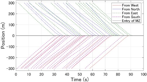
Below are the simulation results presented graphically. Figures 10 and 11 illustrate the input data for each CAV. Meanwhile, Figures 12 and 13 depict the velocity of each CAV. In the position graph, representing Figures 14 and 15, the central point corresponds to the MZ, and the upper and lower boundaries represent the entrances to the CZ. The graph also traces the path of each CAV from its entry into the CZ to its arrival at the central MZ. If the entry is from the north or east, the trajectory is displayed from the top. Conversely, if the entry is from the south or west, the trajectory is shown from the bottom.

Figure 10. Input for each CAV with no Input Correction.

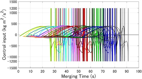
Figure 11. Input for each CAV with Disturbance Observer.

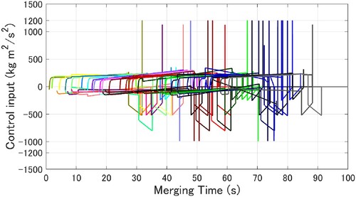
Figure 12. Speed for each CAV with no Input Correction.

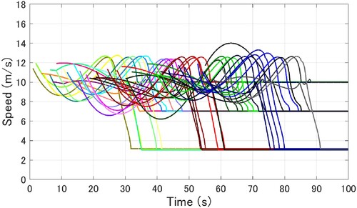
Figure 13. Speed for each CAV with Disturbance Observer.

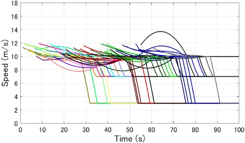
Figure 14. Position for each CAV with no Input Correction.

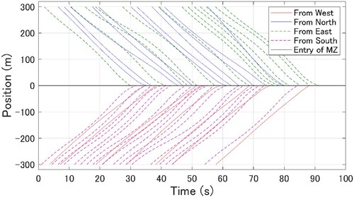
Figure 15. Position for each CAV with Disturbance Observer.

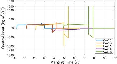
First, Figures 10 and 11 for the inputs show that both input constraints are followed. Now we extract the inputs for 5 of the 50 CAVs, which are shown in Figures 16 and 17.

Figure 16. Input for 5 CAVs with no Input Correction.

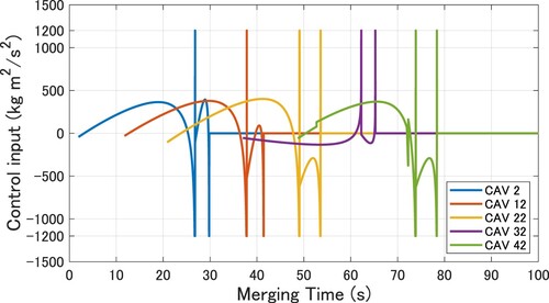
Figure 17. Input for 5 CAVs with Disturbance Observer.

As shown in Figure 16, in the case of no input correction, the input changes significantly, but in the case of input correction using a disturbance observer, as shown in Figure 17, the input changes are suppressed.

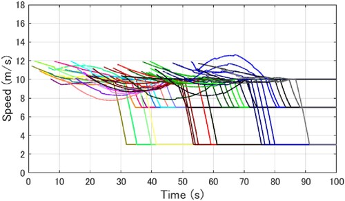
Next, for speed, Figures 12 and 13 show that the speed constraint is observed in both cases. Both graphs show that CAVs pass through the intersection at the terminal speed determined by the right/left turn. Figures 18 and 19 below show the speed trajectories of 5 of the 50 CAVs as in the input case. Figure 18 is the case with no input correction, and Figure 19 is the case with input correction using a disturbance observer.

Figure 18. Speed for 5 CAVs with no Input Correction.

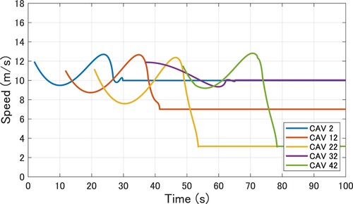
Figure 19. Speed for 5 CAVs with Disturbance Observer.

In case Figure 18, modelling error occurs and the CAV accelerates to meet the merge time $t_i^m$ as it approaches the SRZ, while in case Figure 19, the CAV does not accelerate even near the SRZ and its trajectory is parabolic. These results indicate that the modelling error is suppressed by correcting the input, and that the velocity and position trajectories can be tracked.Finally, the position graphs in Figures 14 and 15 show that no rear-end conflict occurred between CAVs in the same lane. This indicates that the rear-end conflict constraint using the control barrier function is effective, and that the control barrier function is beneficial in addressing the optimal control problem, as it ensures compliance with both speed and input constraints.

The application of optimal control through control barrier functions enables cooperative control without breaching arbitrary constraints. Furthermore, SRZ facilitates CAVs to navigate intersections at specified terminal speeds. Additionally, utilizing a disturbance observer for input correction can effectively mitigate modelling errors.

Next, we simulate a more complex scenario. In the previous example, the slope was assumed to be constant, but as in Figure 20, the slope changes midway through the simulation.

Figure 20. Complex Scenario.

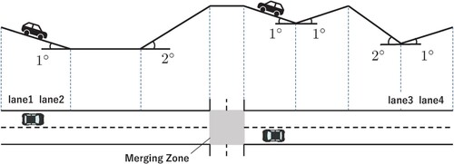
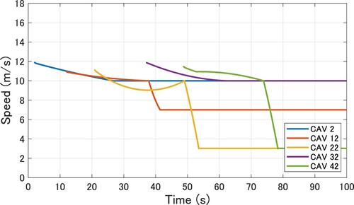
If the vehicle is coming from lane 1 or lane 2, the road starts with a $1^{\circ }$ downhill and then becomes flat. Finally, the road ascends $2^{\circ }$ uphill to reach the intersection. If the vehicle is coming from lanes 3 or 4, it will first $1^{\circ }$ downhill, then $2^{\circ }$ uphill, $1^{\circ }$ downhill, and $1^{\circ }$ uphill, in that order. To verify the effectiveness of the input correction, only the velocity of each CAV with and without the input correction using the disturbance observer is compared. Other conditions remain the same as in Table 2. The results are shown in Figures 21 and 22.

Figure 21. Speed at Complex Scenario (no Input Correction).

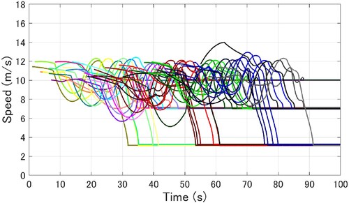
Figure 22. Speed at Complex Scenario (with Disturbance Observer).

Looking at Figures 17 and 18, the results with input correction using a disturbance observer are almost the same as in Figure 13, while the velocity without input correction changes significantly compared to Figure 12. This also demonstrates the effectiveness of input correction in suppressing modelling errors. The input correction using the disturbance observer was also found to be useful for such a complex scenario.

We then examine the computational load: the average computation time for determining the merging time by the coordinator and the average computation time for each CAV, respectively. For the calculations, we used an Intel(R) Core(TM) i5-11400. The results are given in Table 3.

Table 3. Computational load.

Level	Average computation time (s)
Coordinator Optimization	0.0184
CAV Optimization	0.0016

Table 4. Fuel consumption.

Method	Fuel consumption (L)
Proposed	0.9098
Fractional type [18]	0.9758
PI control [19]	0.9332
None	0.9758

The results show that all of them are within the time steps shown in Table 2. The two-stage control structure reduces the computational load and can be applied in the real world.

Finally, we compare with previous studies. In this study we compare fuel consumption with two papers, Xu et al. [18] and Chalaki and Malikopoulos [19]. Both employ optimal control with control barrier functions. However, they employ different input compensation methods. Reference [18] uses an input correction based on the current position and the position of the optimal control solution. The method is expressed as (28) ${\tau }_i^{\mathrm{ref}}\left(t\right)=\frac{p_i^{\ast }\left(t\right)}{p_i\left(t\right)}{\tau }_i^{\ast }\left(t\right)$(28) Reference [19] uses PI control from the viewpoint of speed. The difference between the position and speed of the optimal control solution and the current position and speed is used for the input correction. The method is expressed as (29) $\begin{array}{rl}{\tau }_i^{\mathrm{ref}}\left(t\right)& ={\tau }_i^{\ast }\left(t\right)+K_p\left(p_i^{\ast }\right(t)-p_i(t\left)\right)\\ & +K_v\left(v_i^{\ast }\right(t)-v_i(t\left)\right)\end{array}$(29) For comparison, we consider four methods: the proposed method with input correction by disturbance observer, the input correction methods from References [18, 19], and no input correction (none). Fuel consumption is calculated as the sum of the fuel consumed by all 50 CAVs. The parameters are the same as in Table 2. In this study, we compare these input correction methods. Note that only the input correction methods are compared in Reference [18, 19], since both assume a two-lane intersection and direct comparison is difficult. The gains of the PI controller were set to $K_p=\mathrm{35,000}$ and $K_v=\mathrm{30,000}$. The fuel consumption calculation method is based on Reference [25].

The results are shown in Table 4.

It can be seen that the proposed method has the lowest fuel consumption. The results from the Fractional type [18] are not significantly different from those of the case without input correction. For the PI control method [19], it can be seen that the fuel consumption is reduced by the input correction. The above demonstrates the effectiveness of input correction using a disturbance observer.

6. Conclusion

This study proposed a safe cooperative control algorithm for CAVs at unsignalized intersections that takes into account more realistic conditions such as air resistance and road surface environment. Specifically, we proposed a method for optimal control that avoids conflicts with other vehicles while preserving the vehicle's own constraints such as input and speed by using a control barrier function, a method for input compensation using a disturbance observer to suppress modelling errors, and a method for passing through an intersection at a predetermined terminal speed by setting up a speed regulation zone.

Future works include operation in mixed traffic scenarios with HDV (human-driven vehicle) and CAVs, reduction of the computational load by decentralization, and consideration of uncertainties such as communication errors and delays.

Disclosure statement

No potential conflict of interest was reported by the author(s).

Additional information

Notes on contributors

Yuta Nakai

Yuta Nakai a student of engineering, writes on control theory and on traffic control in the public sphere. Among his recent publication is Cooperative Control of CAVs Using Control Barrier Function at Signal-free Intersection Considering Real Environment (SICE 2023).

Toru Namerikawa

Toru Namerikawa a professor of control theory, writes on control of cyber physical human systems in the public sphere. Among his recent books are Advanced Data Analytics for Power Systems (Cambridge 2021) and Economically Enabled Energy Management: Interplay Between Control Engineering and Economics (Springer 2020).

References

- Ministry of Land, Infrastructure, Transport and Tourism: WHITE PAPER ON TRAFFIC SAFETY IN JAPAN. 2022. Available from: https://www8.cao.go.jp/koutu/taisaku/r04kou-haku/index-zenbun-pdf
- Ministry of Land, Infrastructure, Transport and Tourism: Basic policy for “initiatives to use roads wisely” centered on expressways. Available from: https://www.mlit.go.jp/policy/shingikai/road01-sg-000218
- Zhong Z, Nejad M, Lee EE. Autonomous and semiautonomous intersection management: a survey. IEEE Intell Transp Syst Mag. 2021;13(2):53–70. doi: 10.1109/MITS.2020.3014074
- Mohamad Nor MH, Namerikawa T. Optimal motion planning of connected and automated vehicles at signal-free intersections with state and control constraints. SICE J Control Meas Syst Integr. 2020;13(2):30–39. doi: 10.9746/jcmsi.13.30
- Bian Y, Li SE, Ren W, et al. Cooperation of multiple connected vehicles at unsignalized intersections: distributed observation, optimization, and control. IEEE Trans Ind Electron. 2020;67(12):10744–10754. doi: 10.1109/TIE.41
- Malikopoulos AA, Cassandras CG, Zhang Y. A decentralized energy-optimal control framework for connected automated vehicles at signal-free intersections. Automatica. 2018;93:244–256. doi: 10.1016/j.automatica.2018.03.056
- Medina AIM, van de Wouw N, Nijmeijer H. Cooperative intersection control based on virtual platooning. IEEE Trans Intell Transp Syst. 2018;19(6):1727–1740. doi: 10.1109/TITS.2017.2735628
- Fayazi SA, Vahidi A. Mixed-integer linear programming for optimal scheduling of autonomous vehicle intersection crossing. IEEE Trans Intell Veh. 2018;3(3):287–299. doi: 10.1109/TIV
- Li N, Yao Y, Kolmanovsky I, et al. Game-theoretic modeling of multi-vehicle interactions at uncontrolled intersections. IEEE Trans Intell Transp Syst. 2022;23(2):1428–1442. doi: 10.1109/TITS.2020.3026160
- Chouhan AP, Banda G. Autonomous intersection management: a heuristic approach. IEEE Access. 2018;6:53287–53295. doi: 10.1109/ACCESS.2018.2871337
- Belkhouche F. Collaboration and optimal conflict resolution at an unsignalized intersection. IEEE Trans Intell Transp Syst. 2019;20(6):2301–2312. doi: 10.1109/TITS.6979
- Murgovski N, de Campos GR, Sjöberg J. Convex modeling of conflict resolution at traffic intersections. In: 54th IEEE conference on decision and control (CDC); 2015. p. 4708–4713.
- Katriniok A, Sopasakis P, Schuurmans M, et al. Nonlinear model predictive control for distributed motion planning in road intersections using PANOC. In: 58th IEEE conference on decision and control (CDC); 2019. p. 5272–5278.
- Molinari F, Raisch J. Automation of road intersections using consensus-based auction algorithms. In: Proc American control conference (ACC); 2018. p. 5994–6001.
- Kumaravel SD, Malikopoulos AA, Ayyagari R. Optimal coordination of platoons of connected and automated vehicles at signal-free intersections. IEEE Trans Intell Veh. 2022;7(2):186–197. doi: 10.1109/TIV.2021.3096993
- Antonio G-P, Maria-Dolores C. Multi-agent deep reinforcement learning to manage connected autonomous vehicles at tomorrow's intersections. IEEE Trans Veh Technol. 2022;71(7):7033–7043. doi: 10.1109/TVT.2022.3169907
- Kuchiki A, Namerikawa T. Cooperative control of connected and automated vehicles at signal-freeintersections considering passenger comfort. In: 61st annual conference of the society of instrument and control engineers (SICE); 2022. p. 909–914.
- Xu H, Xiao W, Cassandras CG, et al. A general framework for decentralized safe optimal control of connected and automated vehicles in multi-lane signal-free intersections. IEEE Trans Intell Transp Syst. 2022;23(10):17382–17396. doi: 10.1109/TITS.2022.3151080
- Chalaki B, Malikopoulos AA. A barrier-certified optimal coordination framework for connected and automated vehicles. In: 61st IEEE conference on decision and control; 2022. p. 2264–2269.
- Nakai Y, Namerikawa T. Cooperative control of CAVs using control barrier function at signal-free intersection considering real environment. In: 2023 62nd Annual conference of the society of instrument and control engineers (SICE); 2023. p. 1001–1006.
- Bertsimas D, Tsitsiklis JN. Introduction to linear optimization. Belmont (MA): Athena Scientific Belmont; 1997.
- Blanchini F. Set invariance in control. Automatica. 1999;35(11):1747–1767. doi: 10.1016/S0005-1098(99)00113-2
- Molnar TG, Kiss AK, Ames AD, et al. Safety-critical control with input delay in dynamic environment. IEEE Trans Control Syst Technol. 2022;31(4):1–14.
- Ministry of Land, Infrastructure, Transport and Tourism: Further efficient and effective efforts to reduce traffic accidents. Available from: https://www.mlit.go.jp/common/000221867.pdf
- Kamal MAS, Mukai M, Murata J, et al. Model predictive control of vehicles on urban roads for improved fuel economy. IEEE Trans Control Syst Technol. 2013;21(3):831–841. doi: 10.1109/TCST.2012.2198478