Electric bus arrival and charging station placement assessment using machine learning techniques

ABSTRACT

The goal of this study is to create a dynamic model that can accurately forecast the estimated time of arrival of a bus at a specific bus stop using data obtained from the global positioning system (GPS) in Addis Ababa, Ethiopia. Both operators and customers use accurate and timely bus arrival information. In turn, it helps determine the correct placement of charging stations when green-energy vehicles are introduced in the urban mass transit system. A plethora of machine learning models have been used for prediction. Additionally, we tailored an ensemble method based on the average prediction. The performances of these machine learning methods were estimated and compared using conventional measures, such as Mean Absolute Error (MAE), Mean Squared Error (MSE), Root Mean Squared Error (RMSE), and R-squared (R²) values. The results showed that the performance of the Random Forest technique used in this study was impressive, with MAE of 0.137, MSE of 0.054, RMSE of 0.233, and R² value of 0. 999. The findings demonstrate that the proposed method is reliable for predicting the arrival times of urban and rural buses. Next, in order to position the charging points for Electric Vehicles (EV) along specific bus routes, self-organising map (SOM) is employed to optimise EV charging point placement locations, and the result signify better performance than the kNN and DBSCAN clustering approaches.

KEYWORDS:

• Electric vehicle
• charging points
• arrival prediction
• machine learning
• ensemble technique
• SDG 4
• SDG 7

1. Introduction

1.1. Background

For a long time, public transportation services, such as buses and railroads, relied only on static timetables to plan their trips. Passengers and operators had no means of knowing whether their buses were running late, early, or on schedule. In the 1960s, the first vehicle tracking systems were trailed in Germany and the United States of America (Dhivyabharathi, Anil Kumar, and Vanajakshi 2016). Early systems relied on sensors placed along the route that the bus could detect, allowing it to supply the service provider with real-time location information (Furth 2000).

The modernisation of bus operations and management to focus on supply efficiency and effectiveness in satisfying user needs will be a critical aspect of any strategy to improve public transportation services and use public transportation as a tool for the city’s green growth-oriented initiatives. To reduce the impact on the environment and dependency on fossil fuels, a shift to electric vehicles (EVs) is essential. The provision of effective infrastructure for charging is a crucial component in enabling this shift. With the rise in the popularity of EVs, the transportation sector is experiencing a significant upheaval. It is imperative to address the problem of determining the location of charging stations to meet this shift. Inappropriate positioning of charging stations may affect smooth operation of the power grid causing voltage instability, increased power loss, harmonics and lower reliability indices (Deb et al. 2018). Additionally, charging stations should be easily accessible to EV drivers preferably causing no extra congestion. The use of electric bus arrival prediction is one approach for solving this issue.

The goal of this study is to predict the arrival of electric buses with accuracy so that the right charging station location may be settled on. This is significant because access to charging stations is essential for ensuring the reliability and effectiveness of electric bus services. The location of the charging station can be found, and the bus can be charged at the proper moment by anticipating the arrival of electric buses, ensuring smooth and continuous service.

The most recent research on estimating bus arrival times bases its findings on elements including traffic conditions, the condition of the road system, and the bus schedule (Nanthawichit, Nakatsuji, and Suzuki 2003). However, it is crucial to consider the additional element of choosing the location of charging stations when the use of electric buses increases. By including the features of charging station position determination in electric bus arrival prediction, the current study seeks to advance existing research.

Several methods can be used to attain the objectives of electric bus arrival information and location of charging stations. One such method is the employment of machine learning (ML) algorithms, which can predict the arrival of electric buses by analysing massive volumes of data. The information used in this process can include information on traffic, road networks, transit schedules, and the accessibility of charging stations. In order to assure the reliability and efficiency of electric bus transportation, it can be said that predicting electric bus arrival times and identifying charging stations are essential parts of the transportation sector. The location of the charging station can be determined, and the bus can be charged at the proper moment by accurately forecasting the arrival of electric buses, ensuring a smooth and continuous service.

Intelligent transportation systems (ITS) are transportation services and technologies that aim to improve the efficiency, safety, dependability, and environmental sustainability of transportation systems while avoiding the construction of new infrastructure. Advanced Traffic Management Systems (ATMS), Advanced Vehicle Control Systems (AVCS), Advanced Public Transit Systems (APTS), Commercial Vehicle Operations (CVO), and Advanced Traveler Information Systems (ATIS) are only a few ITS subsystems (Alam, Ferreira, and Fonseca 2016]).

1.2. Motivation

Bus arrival prediction time in public transportation systems is a direct measure of their efficiency and usefulness. Arrival time information is also important in planning operations, route assignments, and determining charging station positions for future electric vehicles.

The design and implementation of ITS tools depend on accurate predictions of arrival by extrapolation of the existing travel time data. In the past, there have been many reports of short-term travel time prediction. These investigations were conducted under homogeneous traffic conditions. Such models and algorithms may not be directly applicable to traffic conditions in Addis Ababa. The traffic in Addis Ababa is heterogenic in composition (Spaliviero and Cheru 2017). A variety of vehicles, two-, three-, and four-wheelers, in addition to a large pedestrian population, share the Addis Ababa urban road (Abebaw 2019). This heterogeneity, coupled with poor lane discipline, makes travel time prediction more challenging when handled using conventional methods. There have been no earlier studies on understanding traffic behaviour under the Addis Ababa road conditions.

Electric buses require access of proper charging stations for charging. Their batteries are heavy, large, and expensive, resulting in a limited driving range (Ullah et al. 2021). Moreover, charging infrastructure is limited, and charging EVs takes a longer time than refuelling diesel vehicles (Liu et al. 2021). These main drawbacks impede EV adoption. Because EVs have limited driving ranges and prolonged charging times duration. To further encourage the use of EVs in the future, a problem that needs to be solved is how to distribute charging stations evenly so that charging stations must be easily accessible at the bus stop point. The importance of Electric bus arrival time is crucial and has direct connection with charging infrastructure. For an example, at a particular junction several buses reach simultaneously and there is single charging station nearby. In this case, there will be a long queue for charging and it is also not possible to accommodate several buses simultaneously as it takes hours for charging heavy vehicles. Hence, we need to understand the density of buses plying in the vicinity of a particular charging station and the nearby stop points. This can be possible by accurately predicting Bus arrival time. The prediction will be also useful for town planners to layout the charging infrastructure.

1.3. Statement of the problem

Electric Vehicles (EVs) have emerged as a mode of transportation free from local emissions. The signatories of the Paris Agreement are planning to use more EVs in the urban transit systems. The use of EVs cannot be successful without a proper charging-station network. In the initial phase of the transition to EV buses in urban mass transit systems, accurate bus arrival prediction will help determine the position of the charging station. The bus arrival prediction in public transportation systems is a direct measure of their efficiency and usefulness. Arrival time information is also important in planning operations, route assignments, and determining charging station positions for future EVs.

1.4. Research questions

In this study, machine learning regression techniques were used to predict bus arrival, and an unsupervised learning algorithm was used to determine the locations of the charging points. Therefore, this study addressed the following research questions:

RQ1:

What are the key factors or features that help develop and predict the bus arrival time prediction model?

RQ2:

Which machine learning algorithm could be used to predict bus arrival time?

RQ3:

How the bus arrival data can be used for placing charging stations?

RQ4:

How to optimise the placement positions of charging points in a city?

Furthermore, the contribution of the paper are as follows:

• We explored the key factors or features of AVL system data that have immense influence on bus arrival prediction model

• We identified the particular machine learning algorithm which is more effective in predicting bus arrival time

• We unearthed how the bus arrival information at the stop points can be useful for effective placement of charging stations.

• We optimised the placement of EV charging points in the Addis Ababa city.

2. Related works

Electric vehicles can help reduce global air pollution and are a promising choice for contributing to greenhouse gas emission reduction goals. However, its success depends on deploying adequate EV charging infrastructure in urban areas. Inappropriate positioning of charging stations may affect smooth operation of the power grid causing voltage instability, increased power loss, harmonics and lower reliability indices. Additionally, charging stations should be easily accessible to EV drivers preferably causing no extra congestion.

The benefits and issue of bus travel time prediction is discussed by Kieu et al. (2012) by highlighting key factors that influence bus transit time. Similarly, another factor, passenger waiting time, at the bus stops when the data is incomplete is studied by McLeod (2007). To this end, Shanthi et al. (2022) developed a web-based application which will be dynamically notify with estimated time of arrival (ETA) of the buses. They used SVR algorithms for prediction.

Liu, Sun, and Wang (2020) proposed a framework for analysing KNN, delay, kernel regression (KR), additive model and RNN based on LSTM for bus arrival time prediction. They used bus schedule data and GPS data in the Dublin city for their analysis. They performed the experiments for 500,10000, 1500 … 4311 bus trips and realised that RNN-LSTM is most efficient one.

Researchers studied a model using a dataset obtained from São Paulo City, which includes bus fleet position data, real-time traffic data, and traffic forecasts from Google Maps (Sloan 2018). They collected geographic data (extensions, bus stops) by cleaning, formatting, and interpreting the data, as well as configuring and training datasets to determine which datasets and hyper-parameters to use and give the best result. Finally, they obtained the bus journey time as forecast after the validation procedure. With the influence of traffic congestion, correlations of the data and the most relevant data for ANN training could be assessed correctly 8.97 present (in comparison, the Nave technique resulted in 12.47 MAPE errors). The stronger the dataset’s correlation, the more precise the prediction, with an error rate of approximately 9%.

Gu et al. (2021) proposed a reliability prediction method to assess the reliability of arrival of bus at stops by using real data of a bus route in Dalian, China. They inferred that accurate online support vector machine (AOSVM) with reasonable parameters can predict the reliability of transit service accurately.

Another study predicted by dividing the problem into two parts: the road travel time and stop time (Wang 2021). Two different models were compared with the (SVR + KNN) method and historical data-based prediction method. The testing findings showed that the (SVR + KNN) method performed better than the historical data-based prediction method for estimating the arrival time of a bus on the same road section. The results showed that the method used in this study was more accurate, with a maximum error of 84 s, a minimum error of 10 s, average relative error of 5.74%, and an average error of 42.5 seconds.

A study compared multiple neural network architectures using historical data and trained three models to predict Boston municipal buses: multilayer perceptron (MLP), convolutional neural network (CNN), and recurrent neural network (RNN) in order to predict Boston municipal buses. Furthermore, model traffic networks employ historical, statistical, and learning-based models, with learning-based models employing GPS data from buses, including latitude, longitude, route, and direction. As a result, the MLP and CNN architectures achieved similar accuracy of 0.88 and 0.85, respectively, but the RNN architecture achieved the best coefficient of determination of approximately 0.89.

The researchers relied on the use of Support Vector Machine (SVM) models to predict bus arrival times tested with real data and compared it with three other models: k-NN (k-nearest neighbours), ANN, and LR. The raw data were collected from public transport providers, including bus ID, time, current location (latitude and longitude), heading, average speed, number of boarding/alighting passengers at bus stops, and so on from a bus route in Dalian, China. The results showed that the SVM models had high accuracy in predicting the bus arrival times.

Another study employed AVL data and passenger flow data (Prakash et al. 2019) of four bus routes of Auckland city, performed both time series and regression based analysis and concluded that time series ANN provided more promising result about bus arrival prediction.

Gurmu looked at numerous ways to predict journey time, including historical and real-time approaches, statistical techniques, machine learning techniques, and model-based techniques (Gurmu 2010). Zhou et al. (2019) developed a bus arrival time prediction model using raw data from Jinan Public Transportation Corporation in Jinan, China, using various traffic data such as line number, bus identification, station number, arrival time, departure time, length of the road segment, number of intersections, number of lanes, and number of passengers. The RNN, SVM, Kalman filter, and MLP were employed for experimentation. They revealed that prediction accuracy of RNN with an attention mechanism is better than RNN with no attention mechanism. Another interesting study find total travel time involving multiple bus trips (He et al. 2018), taking into account riding time, waiting time at the transfer points. They developed the framework and the developed a LSTM model for accurate prediction.

In a study of analysing road accident (Beshah and Hill 2010), they studied severity of accident and its relation with road characteristics by using sevaral ML classification algorithms. We consolidated the extracts of related works and are presented in Table 1.

Table 1. Summary of literatures pertaining to bus arrival prediction.

Studies	ML algorithms used	Best performing algorithm	Performance
Beshah and Hill (2010)	DT,NB,KNN	KNN	AUC-0.965 Accuracy-80.8%
Gu et al. (2021)	AOSVM, KNN, LR and ANN	AOSVM	MAPE- 9.9%
Liu, Sun, and Wang (2020)	RNN-LSTM, KR, KNN Delay and Additive	RNN-LSTM	LSTM > KR > k-NN > Delay > Additive
Wang (2021)	SVR, KNN	SVR+KNN	Maximum error of 84 s, a minimum error of 10 s, an average error of 42.5 s, average relative error of 5.74%.
Shanthi et al. (2022)	SVR, RFR, DTR, KNNR,GBR	SVR	Error value of 30 secs
Zhou et al. (2019)	RNN, SVM, MLP	DARNN	MAE and RMSE of DARNN is better than LSTM-RNN
Prakash et al. (2019)	DT,GEP-TS, GEP-REG,ANN-TS,ANN-REG and MLR	Time series ANN	MAE-10, RMSE-19
Li et al. (2017)	Three stage mixed model involving KNN, Kalman Filter and Markov model	Single step model	MAPE − 0.3
Treethidtaphat et al. (2017)	Deep neural network(DNN)	DNN	MAPE-0.55
Ou (2022)	LSTM	LSTM	MAE- 0.5 min, RMSE-0.72 min
Fan and Gurmu (2015)	Historical average, Kalman Filtering and ANN	ANN	Average MAPE- 8.5%

For EV charging, a study used a multi-objective framework considering the economic factors and power grid characteristics, such as voltage stability, reliability, and power loss, as well as EV user convenience and random road traffic to determine the position of the charging station (Deb et al. 2019). Another study employed the multiple criteria decision-making (MCDM) method in a Pythagorean fuzzy environment to determine the position of the charging station (Yang et al. 2021). Furthermore, the application of machine learning to determine EV charging station positions has been studied by several authors (Kalakanti and Rao 2022). A recent study by Ullah et al (2023) examines EV charging station choice behaviour and aims to find the best prediction method. This study suggests that combining ML models with SHAP (SHapley Additive exPlanations) (Lundberg and Lee 2017) has the potential to develop an interpretable ML model for predicting EV charging station choice behaviour and determining most important factors for normal and fast charging stations. They used ML algorithms (LR, NB, RF, and XGBoost) to train and test the data and revealed that XGBoost model outperformed other ML models.

From the existing literature review, we concluded that several literatures are availble pertaining to bus arrival time prediction using ML techniques. Further, few authors are also discussed charging station placement in a particular study area. However, our research aims to connect arrival time estimation with laying down charging infrastructure in the study area.

3. Methodology

This section details how the data were collected, the understanding of the collected data, feature selection, preprocessing such as data cleaning, data formatting, and methodologies that have been used for model building.

3.1. Data collection

Automatic Vehicle Location (AVL) systems were used to collect the dataset. GPS receivers are commonly interfaced with GSM modules and are installed in buses in these systems. They primarily keep records of point locations in latitude-longitude pairs, bus speeds, and date and time daily, from 6:00 AM to 7:30 PM. The most important records were the arrival and departure times at each bus stop. A snapshot of the data-collection scheme is presented in Figure 1. Information was gathered from Sheger Public Transport, Addis Ababa, Ethiopia, for a period of one year.

Figure 1. Data collection scheme in the study area.

A snapshot of data collection framework for the study area.

3.2. Business process understanding

In many cities, public bus services are still the most common mode of transportation, and millions of people rely on them every day to reach their destinations. However, in many places, this service is known for its unpredictable scheduling and substantial time differences. While the system is inherently dependent on external elements that cannot be controlled, such as traffic and weather, some infrastructure enhancements can be made in an attempt to reduce concerns and provide a better experience for riders.

Public transport systems are increasingly equipped with information and communication technologies such as automatic vehicle location (AVL) and automatic passenger counts (APC). Many AVL systems, designed primarily for real-time applications, fail to capture and/or archive data items that would be valuable for off-line analysis (Cats and Loutos 2016). Moreover, off-line analysis has different data needs than online (real-time) monitoring. Hence, AVL systems designed for real-time monitoring may not deliver the type and quality of data needed for offline analysis. Considering the ways off-line data can be used to improve operations and management, and considering the way AVL system design affects what data is captured as well as its quality, Furth et al (2006) presents findings related to AVL system design. Most off-line analyses, including analyses of running time and schedule adherence, require knowledge of departure time from standard locations. Therefore, stop and timepoint records are inherently better suited to off-line analysis of AVL data

Several cities across the globe have begun to implement real-time monitoring systems that track the locations of each bus in their fleet and make that information public via the internet. This study describes the process for converting real-time vehicle data into a format suitable for machine learning as well as the strategies utilised to generate precise vehicle arrival time predictions from GPS data.

The data used in this study were collected from the Sheger bus services in Addis Ababa, Ethiopia, which operate and manage both public and private transportation. TransLink operates a fleet of 20 buses on approximately 123 routes, many of which are fitted with the AVL system, which tracks each bus’s precise GPS coordinates. The complete bus route is illustrated in Figure 2. However, alternative public transportation options, such as the Anbessa bus and other Sheger buses, have no fleet management and still use manual systems.

Figure 2. Bus route in the city.

Complete Bus Route in Addis Ababa city.

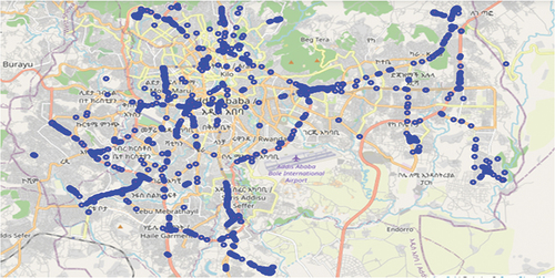
The complete bus route of the city is shown in Figure 2.

3.3. Feature selection

The process of producing a subset from an initial feature set according to a feature selection criterion that selects the relevant features of the dataset is known as feature selection. It aids in the compression of data-processing scales by removing superfluous and extraneous characteristics. Learning algorithms can be preprocessed using feature selection techniques, and effective feature selection results can enhance learning accuracy, shorten learning time, and simplify learning outcomes (Acharjya and Das 2017).

In this study, more relevant features that might help develop a bus arrival time prediction model were identified. Features from the GPS data that were irrelevant for this study were removed based on domain experts’ suggestions.

According to domain experts, the 11 variables listed in Table 2, including the dependent feature, were identified as the most important features for bus arrival time prediction. These features are believed to play a role in predicting actual bus arrival times. Consequently, the model building was based on the 11 most important features.

Table 2. Description of the selected features.

No.	Features Name	Data Type	Description
1	Beginning Date	Numerical	Initial Date of the trip
2	Beginning Time	Numerical	Initial Time of the trip
3	End Date	Numerical	End Date of the trip
4	Peak/off peak	Categorical	Shows the time of crowding/traffic congestion
5	Mileage	Numerical	Total distance in kilometer of the trip
6	Duration	Numerical	The difference between the projected arrival time and the actual arrival time
7	Initial latitude	Numerical	Source Latitude of vehicle
8	Initial longitude	Numerical	Source Latitude of vehicle
9	Final latitude	Numerical	Destination Latitude of vehicle
10	Final longitude	Numerical	Destination Latitude of vehicle
11	End Time	Numerical	End Time of the trip

3.4. Data preprocessing

Replacing, changing, or deleting dirty or noisy data is the process of finding and fixing (or removing) corrupt or inaccurate entries in a record set, table, or database. However, there were no missing data or outlines in the collected dataset. In the event of data containing noise, techniques for data cleaning and imputation can be incorporated into the model. In general, most AVL systems generate data, which are not free from anomalies (Barabino, Di Francesco, and Mozzoni 2013, 2017). Furthermore, various architectures for AVL-based systems are also being employed for capturing vehicular information (Dhurandher et al. 2010; Hounsell and Shrestha 2005). In the case of data consisting missing values, outliers can be easily handled in the data pre-processing phase

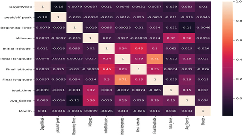
Tasks, such as reducing the number of feature attribute values and tuples, are integrated into this technique. These activities can be performed in various ways. Some of these tasks were performed in this study. For example, irrelevant features were removed from the feature selection section. After applying data cleaning and obtaining the cleaned dataset, a significant dependency or association between the independent variables or predictor variables must be considered to confirm the presence or absence of multi-collinearity. From Figure 3, it can be concluded that there was no multicollinearity in the features. Therefore, all features were considered when building the model.

Figure 3. Feature correlation (heat map).

Features present in the data and correlation between them.

The process of converting data into a format suitable for model building involves data transformation (data consolidation). In this section, the selected data features are transformed into the most suitable format for training the machine-learning algorithms. Among the selected features, one was categorical, and the remaining attributes were numerical. This type of mixed data causes problems in ML algorithms. Hence, the categorical feature (peak/off-peak) was changed to a numerical value using the label encoding technique. The dataset also contained features with date and time formats. These features should be changed to a more suitable format for the model. Hence, the features are converted into numeric values. The module is used to transform the date into weekday, month, and year and the time into hourly numerical values.

3.5. Performance evaluation metrics

The following four measures were used to assess regression model performance: Mean Absolute Error (MAE), Mean Square Error (MSE), Root Mean Squared Error (RMSE), and R-squared (R²) (Bebarta et al. 2021). The fraction of variation in the observed data explained by the model is denoted as R². Normally, R² takes values between zero and one. Closer values of 1 are better because the model explains more of the variance.

The MAE is a measure of the differences in errors between paired observations that reflect the same phenomena. Comparisons of predicted versus observed, subsequent time versus starting time, and one measuring technique versus other measurement techniques are examples of Y versus X. Equations (1) to 4 represent the formulas for the MAE, MSE, RMSE, and R², respectively.

(1) $\mathit{MAE}=\frac{1}{n}{\sum }_{i,j=1}^n\left|y_j-y_i\right|$(1)

MSE is a metric that evaluates the difference between the expected and desired solutions, and may be calculated using (2).

(2) $\mathit{MSE}=\frac{1}{n}{\sum }_{i,j=1}^n{\left(y_j-y_i\right)}^2$(2)

where y_i is the predicted value of instance j; y_j is the real target value of instance j; and n is the total number of instances.

The RMSE measures the difference between known and interpolated or digitised places. The RMSE is calculated by combining the differences between the known and unknown points, dividing by the number of test points, and calculating the square root of the result.

(3) $\mathit{RMSE}=\sqrt{\frac{1}{n}{\sum }_{i,j=1}^n{\left(y_j-y_i\right)}^2}$(3)

R² Score: For model validation, the coefficient of determination (R²) between the outcome and predicted values was also used. Equation (4) was used to compute the coefficient of determination (R²).

(4) $R^2=\frac{\mathit{S}{\mathit{S}}_{\mathit{reg}}}{\mathit{S}{S}_{\mathit{tot}}}=\frac{{\sum }_j{\left(y_j-\bar{y}\right)}^2}{{\sum }_i{\left(y_i-\bar{y}\right)}^2}$(4)

where the predicted labels are denoted by yj, and the genuine labels are denoted by yi. where SStot is the total sum of squares, which is proportional to the variance of the data, and SSreg is the regression sum of squares.

3.6. Proposed model

As illustrated in Figure 4, the system architecture initiates with the collection of GPS data, followed by converting the acquired Excel file data into CSV format. The dataset is used for feature selection. From the selected feature the ordinal values are subsequently quantified. In the preprocessing the features like total time and distance are derived. The resulting dataset consists of features DayofWeek, peak/off peak, Beginning Time, End Time, Mileage, Initial latitude, Initial longitude, Final latitude, Final longitude, total_time, Avg_Speed, Month and distance.

Figure 4. Proposed machine learning model.

Proposed framework for testing with individual and ensemble-based regression models.

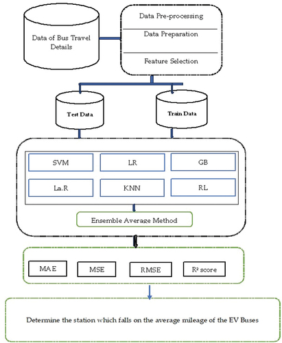
Next, the prepared dataset is partitioned into training and testing sets with a ratio of 90% for training and 10% for testing. The model is train using training dataset. Various algorithms including Random Forest, Gradient Boosting, Linear Regressor, Lasso Regressor, K Nearest Neighbor, and Support Vector Regressor are trained. The performance of the models is assessed using metrics such as R2, MAE, RMSE, and MSE during the model evaluation step. Following evaluation, the algorithm having high accuracy results is selected. Finally, the chosen best model is deployed to forecast bus arrival times. This arrival time is used to identify stations that fall within the range of the average milage of the EVs.

Once the bus arrival data are in hand, we use it for charging station installation for urban mass transit systems. The station location was determined by considering the average milage of the EV vehicle in full charge. The bus stations near the average milage of the EV can serve as potential charging stations.

3.7. Charging station location identification

Bus arrival prediction information and average bus mileage were used to select the location of the charging station. This information was also used to determine the delay of the vehicle in the charging station once the charging stations were set.

This research uses Self-Organizing Maps (SOMs) to identify possible EV charging-point clusters. SOMs are a type of artificial neural network that use similarity to arrange data. In this case, SOMs assist in identifying areas with high-density paths, suggesting ideal sites for charging stations. Every route was mapped to a particular neuron on the SOM grid, and the SOM algorithm was trained using this dataset. Every neuron in the dataset represents a distinct area once training is completed. By examining these neurons, we can find clusters of paths that indicate good places for EV charging stations. With this strategy, it is possible to determine the best charging locations based on route density and dispersion using a data-driven approach. The operational steps of this process are listed in Table 3.

Table 3. Description of charging point selection steps.

Sl. No of Steps	Descriptions
Step 1. Data Collection	Gather dataset with route information
Step 2. Data Preprocessing	Clean, format date/time, ensure coordinates are numeric
Step 3. Exploratory Data Analysis (EDA)	Gain insights from dataset
Step 4 Feature Engineering	Create useful features if needed.
Step 5 Clustering Algorithm Selection	Choose K-Means, DBSCAN, or SOM.
Step 6 Apply Clustering Algorithms	Identify potential charging points.
Step 7 Visualize Clusters	Plot routes and clusters
Step 8 Select Optimal Points	Identify strategic locations based on clustering.
Step 9 Additional Filtering	Apply extra criteria.
Step 10 Map Visualization	Plot charging points on real map.
Step 11 Evaluation and Validation	Assess charging points based on criteria.
Step 12 Final Selection	Choose optimal EV charging points
Step 13 Generate Reports	Summarize process, criteria, and recommendations.

The first stage was a comprehensive preparation of the data, which included managing missing values, translating formats for dates and times, and identifying pertinent characteristics for the analysis. For consistency, the latitude and longitude coordinates were standardised.

4. Experimental result and discussion

The tools used for implementation were installed on a personal computer with an Intel® Core™ i7-8750 H CPU @2.20 GHz, 2208 Mhz, 6 Core(s), 12 Logical Processor (s), 16 Gigabytes of RAM, 18.8 Gigabyte of total virtual memory, and 500 Gigabytes hard disk storage capacities. The operating system is Windows 10 Enterprise, 64 bits.

4.1. Preliminary analysis

Before building the machine learning model, additional features that helped the model were derived from the collected GPS data. The derived features are discussed as follows.

4.1.1. Time series analysis

In this study, time is an important feature because it reveals how the data change over time, and the final outcome is also a time feature. Hence, all the time and date features in the dataset were handled using the Python datetime function. It helps to transform the date into month, day, and year, and time into minutes, hours, and seconds. In addition, the beginning and end times were changed to hours.

4.1.2. Deriving average speed of the bus

The average speed is one of the factors that might influence the final arrival time of the bus. It was derived by subtracting the start time from the end time and dividing the mileage by the total time. After deriving the average speed, the dataset was increased with a new column called Avg_Speed, as shown in Figure 5. The average speed plays a vital role in determining the position of a charging station.

Figure 5. Dataset after adding average speed.

A snapshot of the Dataset with average speed attribute.

4.1.3. Calculating distance between two locations

Because one bus travels from one initial location to a predetermined destination, it is possible to calculate the distance travelled using the Haversine distance formula. The Haversine distance formula determines the great-circle distance between two locations on a sphere using geolocation information (longitude and latitude). This was performed using a Python module called haversine. The Python function calculates the distance a bus travels from the initial location (using the initial latitude and longitude) to the final location (using the final latitude and longitude).

Figure 6 shows the dataset after calculating the haversine distance between the initial and final locations of the bus trip.

Figure 6. Dataset after distance calculation.

A snapshot of dataset with Haversine distance between initial and final locations.

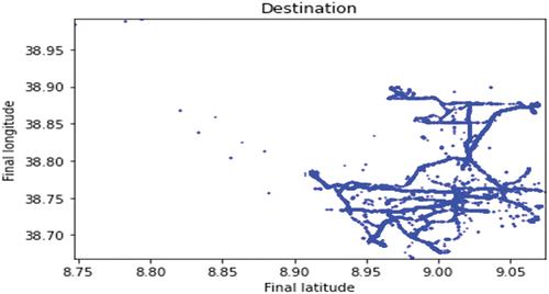
The dataset covers areas with a minimum latitude and longitude range of (8.74698, 38.668259) and a maximum range of (9.07393, 38.990913), as shown in Figure 7.

Figure 7. Bus trip locations.

Bus trip localization with latitude and longitude.

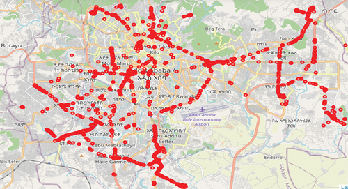
Based on the GPS data, the buses cover and travel 123 routes, as shown in Figure 8.

Figure 8. Bus trip routes.

Complete Bus Trip Routes in the Addis Ababa city.

4.2. Feature scaling

Because of the highly diverse range of input features, the data must be scaled before being fed into the model. For example, the duration range can be tens to thousands of seconds, with 1 and 0 representing the peak and off-peak hours, respectively. Large differences in the input features might lead to a fitting problem because a feature with a large number may be given different weights than a feature with a small number. To improve the prediction model, min-max scaling was utilised to scale the value of the data between 0 and 1 in this study.

4.3. Model building

The dataset must be split into training and testing sets to make the model more efficient by training the model using the training set and then evaluating its performance using the testing set. Therefore, from the total 140,589 instances of the data, 90% were used for training and 10% for testing purposes.

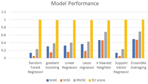
After completing all necessary data preparation and preprocessing steps, the next step is to build the model, which is the main aim of this research. Six different machine learning regression algorithms were selected to develop the models, and the model that achieved the best performance was selected as the best model. Additionally, we created an ensemble average by considering these six models. Table 4 illustrates the model training and evaluation results of each developed model, that is, random forest, gradient boosting, linear regression, lasso regression, k-nearest neighbour, support vector regressor, and ensemble averaging (Mohapatra et al. 2021). The details of the execution time, R² score, MAE, MSE, and RMSE of all seven models are presented in Table 4.

Table 4. Execution time, R² score, MAE, MSE and RMSE of each Model.

Model Name	Execution Time (In Second)	MAE	MSE	RMSE	R^2 score
Random Forest Regressor	179.254699	0.13677	0.05404	0.23247	0.9995
Gradient Boosting	45.98444605	0.304526	0.149515	0.386671	0.99039
Linear Regressor	6661.479553	0.324486	0.162654	0.403303	0.989363
Lasso Regressor	4257.271728	0.364665	0.182817	0.427571	0.987939
K- Nearest Neighbor	7054.738146	0.469807	0.463268	0.680638	0.979969
Support Vector Regressor	7651.254699	0.136771	0.054043	0.232471	0.999496
Ensemble Averaging	7657.145359	0.494396	0.473161	0.691622	0.999967

4.4. Model comparison and discussion

The fact that the dataset used in this study did not have any missing values or outliers and a large number of instances helped stabilise the performance of the model. All models achieved very interesting scores. However, from the selected algorithms, the model built with Random Forest (RF) achieved the best result compared to the other six techniques by achieving a lower error value and a very high R² score because when the determinant factor approaches 1, the model can predict the value by having a lower error rate. The performance of all six regression models, along with the ensemble average model, is shown in Figure 9.

Figure 9. Comparison of models’ performances.

Performance Comparison of all the Six Models’ and Ensemble model.

4.5. Model testing

As illustrated in Figure 9, the random forest regressor model outperformed the other models by achieving less error. Therefore, in this phase, the model is tested, and predictions are made using unseen/test data.

The model testing results depicted in Figure 10 demonstrate that the model built with the RF regressor model predicts the arrival time with less error. Therefore, it can be concluded that the RF algorithm can be used to predict the arrival times of buses in Addis Ababa City.

Figure 10. Model testing result.

Testing Result of Random Forest model.

4.6. Regression analysis

We conducted linear regression to assess the predicted bus arrival time with the actual arrival time. In the equation y = ax+ b, y is the predicted value and x is the actual value. The results of the regression were tested using the standard error(SE), p-value(p), and t-value(t).

The value of ‘A’ in Table 5 is close to 1, and the SE value is relatively small, indicating that the predicted value is very close to the real value. The p value for ‘A’ is below the standard 0.05 and the t for ‘A’ is very high. This indicated the accuracy of the model. The correlation between the predicted and actual models is shown in Figure 11. The points were very close to the regression line, indicating a positive correlation between the actual and predicted values.

Figure 11. Predicted and actual values of different models.

Predicted and actual values as generated by various models (A) Random Forest (B) Gradient boosting (C) Linear Regressor (D) Lasso Regressor (E) K Nearest Neighbor (F) Support Vector Regressor (G) Ensemble Averaging model.

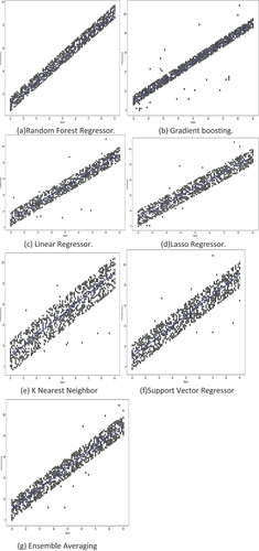
Table 5. Linear regression analysis of the individual models.

Model	Parameter	Approximated Value	SE	p	t
Random Forest Regressor	A	0.9913	0.005	0	187.342
	B	28.5336	16.121	0.75	1.86
Gradient boosting	A	1.0012	0.06	0.098	176.143
	B	−12.2083	153.165	0.931	−0.08
Linear Regressor	A	0.9844	0.005	0	192.189
	B	44.7213	16.195	0.006	2.762
Lasso regressor	A	0.9099	0.005	0	196.178
	B	104.2845	62.836	0.098	1.66
K Nearest Neighbor	A	0.9876	0.05	0	179.143
	B	−13.1023	149.135	0.9021	−0.08
Support Vector Regressor	A	0.9612	0.005	0	189.189
	B	45.3421	16.005	0.006	2.3001
Ensemble	A	0.9311	0.005	0	183.184
Averaging	B	46.0421	15.005	0.006	2.2001

Once the arrival time is accurately predicted, using the average speed of the electric vehicle, we can locate the position of the charging station in the urban mass transit system.

4.7. Feature important analysis based on SHAP

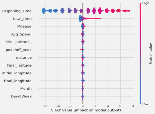
SHAP (Shapley Additive Explanations) helps to understand impact of features on decision variable. We used SHAP to assess the relative importance of features in predicting the arrival time. A higher value of SHAP indicate that the independent variable has significant impact on the determination of dependent variable.

From Figure 12, clearly, day of week, month, final latitude have very less effect on the bus arrival estimation. Distance, has both positive and negative SHAP value but the magnitude is not so much. However, peak hour has a positive SHAP value on the prediction. Beginning time, has both positive and negative SHAP values and it is highly influencing factor for the arrival time prediction.

Figure 12. Variables and their SHAP values of the random forest model.

SHAP analysis results for the Random Forest model.

4.8. Charging station location identification

Self-Organizing Maps (SOMs) play a vital role in optimising EV charging point placement by analysing large datasets and unlike static models, SOMs continuously learn and adjust as new data becomes available, reflecting evolving EV adoption rates, user preferences, and infrastructure changes. Their grid-based structure offers an intuitive understanding of cluster distribution, facilitating informed decision-making and communication with stakeholders. They group areas with high EV ownership, driving patterns, population density, and charging station usage, pinpointing locations with strong charging point needs. Therefore, SOMs offer a powerful tool for optimising EV charging point placement, contributing to a more efficient, equitable, and sustainable EV charging infrastructure.

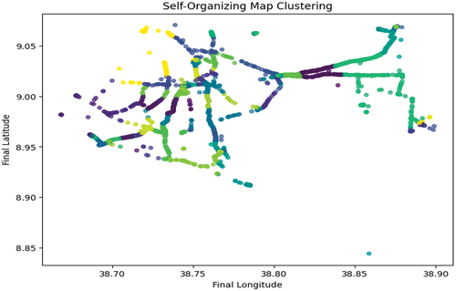
Using SOMs, an unsupervised learning method (Raptodimos and Lazakis 2018), high-dimensional data can be shown on a 2D grid while maintaining its underlying structure. In this study, the best locations for EV charging stations were identified by grouping bus routes according to their final coordinates using SOMs, as presented in Figure 13.

Figure 13. Bus routes according to their final coordinates.

Bus routes and self-organising map clustering schema.

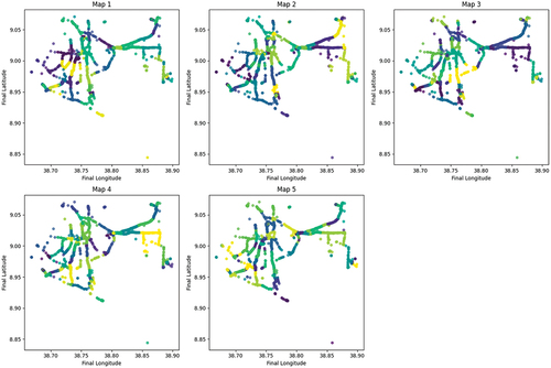
The bus routes were clustered into discrete groups using the SOM method; each group represented a possible site for an EV charging station. The results are shown graphically on a map to aid comprehension and judgement. According to various clusters of data for bus routes, possible maps are shown in the maps presented in Figure 14.

Figure 14. Maps according to possible cluster of the data for bus routes.

Varied generated Maps according to possible charging station placements.

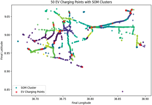
Promising findings were obtained from SOM clustering, which was able to locate groups of bus routes with comparable end locations. Considering route popularity and geographic dispersion, our clustering technique offers insightful information regarding possible locations for EV charging stations. In Figure 15, the optimal locations for the EV charging points are shown as a red cross. The SOM clustering method identified 50 points for the EV charging stations.

Figure 15. Possible locations for EV charging stations according to SOM.

Possible locations for EV charging stations as resulted by applying SOM.

Comparison with K-means and DBSCAN: We compared the outcomes with those of more conventional clustering techniques, such as K-means and DBSCAN, to verify the efficacy of the SOM methodology. The SOM approach performed better than the others, demonstrating its applicability to this particular optimisation problem. A comparison of the clustering performance is shown in Figure 16.

Figure 16. Comparative clustering performances.

Comparison of various clustering performances (a) Silhouette score based comparision (b) Number of clusters (c) Silhouette score vs Homogeneity score.

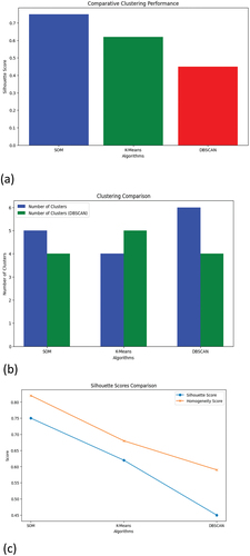
The performance of SOM depends upon grid structure, aids in understanding cluster distribution, adaptation to new data and capturing evolving trends. It has capability to incorporate accessibility, land availability, charger mix, and equity. SOMs continuously learn and adjust as new data becomes available, reflecting evolving EV adoption rates, user preferences, and infrastructure changes. However, KNN and DBSCAN lacks visual representation of clusters, making interpretation challenging. It has also a problem for choosing appropriate density parameters which influences cluster identification.

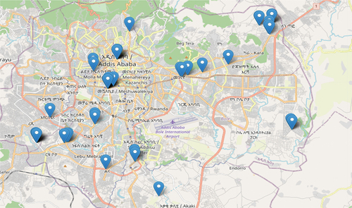
Finally, the charging-point locations are represented in the city map, as shown in Figure 17.

Figure 17. Optimal EV charging point locations in the map of Addis Ababa.

EV charging point locations in Addis Ababa city.

Transportation, particularly bus transportation, is subject to many problems in Addis Ababa, Ethiopia’s capital city. In particular, the arrival time of buses at stations is yet to be predicted accurately. In addition, research conducted elsewhere could not be directly applied to this city because of the unique nature of transportation problems, such as traffic heterogeneity in the composition and variety of vehicles and a large pedestrian population coupled with poor lane utilisation. In addition, the city’s transportation management system involves disintegrated manual systems, which results in poor delivery of transportation services. To overcome these problems, we used ML algorithms (Arhin, Manandhar, and Baba-Adam 2020) together with real-time Global Positioning System (GPS) data to provide a better solution to the existing problem.

The model developed will impact the efficiency and sustainability in the following ways:

• The findings try to reduce the distance that the EV will travel to access the charging station and this impacts the state of the charge of the electric vehicle

• The proper location of the CS reduces the total expected cost of the charging process and increases the EV owner’s convenience.

• A righteous CS need estimation for a region improves the customer satisfaction-involved operational cost, while considering the potential uncertainties

5. Conclusions

It has become increasingly important for modern public transportation to sustain and improve quality of life by providing mobility and accessibility. It is better to have a network of EVes in our urban transit system. It also helps safeguard the environment, promote economic development, and foster social solidarity. Various public transportation improvement ideas have been presented in the past, but they face challenges owing to a lack of travel information. The focus of this study was the use of ML regression techniques for bus arrival time prediction. It is part of the pre-construction work of the charging station for Addis Ababa’s Advanced Public Transportation System. To the best of our knowledge, no attempt has ever been made before for such exercises. For such an APTS system, real-time data-gathering techniques are required for better arrival-time prediction. This arrival prediction can be used to determine charging stations for urban transit. To create the models, GPS data, which were relatively new at the time, and seven ML techniques were employed. Then, the performance of each model is tested and compared to obtain a model that can efficiently predict the arrival time of buses. The overall findings of this study are encouraging and show that the proposed Random Forest model can be used to advance and modernise the public transportation system by predicting bus arrival times at bus stops in the study area with undisciplined traffic flow, particularly since the fleeting monitoring system is new in the area.

Furthermore, the study demonstrates the potential of SOM in optimising EV charging-point placement along specific bus routes. By leveraging unsupervised learning, strategic locations that cater to a wide range of commuters can be effectively identified. Urban planners can use our findings for endorsing charging station placement decisions when many charging stations (in the order of hundreds or more) need to be placed at different locations of a planned area, i.e. considering the clustering efficiency and the EV owner’s convenience. This approach contributes to the sustainable development of the transportation infrastructure and encourages the adoption of electric vehicles. Future endeavours may focus on expanding the scope of the analysis to consider additional factors, such as traffic density, proximity to public amenities, and real-time data feeds. Moreover, collaboration between urban planning authorities and energy providers could lead to the implementation of recommended EV charging points.

Author contributions

Conceptualization, H.R. and S.K.M.; methodology, T.K.D. and S.K.D.; data curation, H.R.; formal analysis, S.K.M.; investigation, S.K.D.; writing – original draft preparation, T.K.D. and S.K.M.; Review and editing, T.K.D. and S.K.D. All authors have read and agreed to the published version of the manuscript.

Disclosure statement

No potential conflict of interest was reported by the author(s).

Data availability statement

The data that support the findings of this study are available from the corresponding author, T.K.Das, upon reasonable request.

Additional information

Funding

No funding was received

Notes on contributors

Habtu Reda

Habtu Reda received his M. Sc (Software Engineering) from Addis Ababa Science and Technology University, Addis Ababa, Ethiopia and a Bachelor’s in software engineering from Micro Link Information Technology College. He is currently working in Addis Ababa City Bus Service Enterprise as Director in ICT directorate and Manager in TRNSIP ITS/ICT World Bank project, Govt. of Ethiopia. His research interest is in Machine Learning applications in e-governance.

Sudhir Kumar Mohapatra

Sudhir Kumar Mohapatra received Ph.D. degree in Computer Science & Engineering from SOA University, Bhubaneswar, India in 2016 and MTech from Utkal University, Bhubaneswar, India in 2011. His research interests are machine learning, software testing, soft computing, regression testing, computational intelligence, and evolutionary computations. He has around 55 research articles in reputed international journals and conferences, 1 book, and 20 book chapters in his credit. He has 15 years of experience in teaching and research. Currently, he is working as an Associate Professor in the Faculty of Engineering & Technology, Sri Sri University, Cuttack, India.

Tapan Kumar Das

Tapan Kumar Das is currently working as a Professor in the School of Computer Science Engineering and Information Systems, Vellore Institute of Technology, Vellore. He graduated from Berhampur University, received M. Tech from Utkal University in 2003, and a Ph.D. degree in Computer Science and Information Technology from VIT University, India in 2015. He has about 20 years of experience in various capacities in the IT industry and academics. He has authored more than 50 journals conference research articles, and book chapters with various reputed publishers. His research interests include Artificial Intelligence, Machine Learning and Data Analytics, Medical informatics, and cognitive computing. He is a senior member of IEEE and, life Member of the Computer Society of India and the Indian Science Congress Association.

Santanu Kumar Dash

Santanu Kumar Dash received the B. Tech degree in Electronics Engineering from Biju Pattnaik University of Technology Rourkela in 2011 and M. Tech from Sambalpur University, Burla, India in 2013. He has received the Ph.D. degree in Electrical Engineering from National Institute of Technology Rourkela, India in 2019. He is now working as Senior Assistant Professor at TIFAC-CORE Research Center, Vellore Institute of Technology, Vellore, India. His research interests include Electric Vehicle, grid connected systems, distributed generations and embedded system application for power converter control.

References

- Abebaw, A. 2020. “Why Should Ethiopians Care About Urbanization? Jobs, Infrastructure, and Formal Land and Housing.” Blog, May 21, 2019. https://blogs.worldbank.Org/africacan/why-shouldethiopians-care-about-urbanization-jobs-infrastructure-and-formal-land-and-housing.
- Acharjya, D. P., and T. K. Das. 2017. “A Framework for Attribute Selection in Marketing Using Rough Computing and Formal Concept Analysis.” IIMB Management Review 29 (2): 122–135.
- Alam, M., J. Ferreira, and J. Fonseca. 2016. “Introduction to Intelligent Transportation Systems.” Intelligent Transportation Systems: Dependable Vehicular Communications for Improved Road Safety 1–17.
- Arhin, S., B. Manandhar, and H. Baba-Adam. 2020. “Predicting Travel Times of Bus Transit in Washington, DC Using Artificial Neural Networks.” Civil Engineering Journal 6 (11): 2245–2261.
- Barabino, B., M. Di Francesco, and S. Mozzoni. 2013. “Regularity Analysis on Bus Networks and Route Directions by Automatic Vehicle Location Raw Data.” IET Intelligent Transport Systems 7 (4): 473–480.
- Barabino, B., M. Di Francesco, and S. Mozzoni. 2017. “Time Reliability Measures in Bus Transport Services from the Accurate Use of Automatic Vehicle Location Raw Data.” Quality and Reliability Engineering International 33 (5): 969–978.
- Bebarta, D. K., T. K. Das, C. L. Chowdhary, and X.-Z. Gao. 2021. “An Intelligent Hybrid System for Forecasting Stock and Forex Trading Signals Using Optimized Recurrent FLANN and Case-Based Reasoning.” International Journal of Computational Intelligence Systems 14 (1): 1763–1772.
- Beshah, T., and S. Hill. 2010. “Mining Road Traffic Accident Data to Improve Safety: Role of Road-Related Factors on Accident Severity in Ethiopia.” In 2010 AAAI Spring symposium series.
- Cats, O., and G. Loutos. 2016. “Evaluating the Added-Value of Online Bus Arrival Prediction Schemes.” Transportation Research Part A: Policy and Practice 86:35–55.
- Deb, S., K. Tammi, K. Kalita, and P. Mahanta. 2018. “Impact of Electric Vehicle Charging Station Load on Distribution Network.” Energies 11 (1): 178. https://doi.org/10.3390/en11010178.
- Deb, S., K. Tammi, K. Kalita, and P. Mahanta. 2019. “Charging Station Placement for Electric Vehicles: A Case Study of Guwahati City, India.” Institute of Electrical and Electronics Engineers Access 7:100270–100282.
- Dhivyabharathi, B., B. Anil Kumar, and L. Vanajakshi. 2016. “Real Time Bus Arrival Time Prediction System Under Indian Traffic Condition.” In 2016 IEEE International Conference on Intelligent Transportation Engineering (ICITE), pp. 18–22. IEEE.
- Dhurandher, S. K., S. Misra, M. S. Obaidat, M. Gupta, K. Diwakar, and P. Gupta. 2010. “Efficient Angular Routing Protocol for Inter-Vehicular Communication in Vehicular Ad Hoc Networks.” IET Communications 4 (7): 826–836.
- Fan, W., and Z. Gurmu. 2015. “Dynamic Travel Time Prediction Models for Buses Using Only GPS Data.” International Journal of Transportation Science and Technology 4 (4): 353–366.
- Furth, P. G., B. Hemily, T. H. Muller, and J. G. Strathman. 2006. “Using Archived AVL-APC Data to Improve Transit Performance and Management.” No. Project H-28.
- Furth, P. G. 2000. “Data Analysis for Bus Planning and Monitoring.” In No. Vol. 34. Transportation Research Board.
- Gu, X., C. Chen, Y. Yang, X. Miao, and B. Yao. 2021. “Reliability Prediction of Further Transit Service Based on Support Vector Machine.” Measurement and Control 54 (5–6): 845–855.
- Gurmu, Z. K. 2010. “A dynamic prediction of travel time for transit time for transit vehicles in Brazil using GPS data.” Master’s thesis, University of Twente.
- He, P., G. Jiang, S.-K. Lam, and D. Tang. 2018. “Travel-Time Prediction of Bus Journey with Multiple Bus Trips.” IEEE Transactions on Intelligent Transportation Systems 20 (11): 4192–4205.
- Hounsell, N. B., and B. P. Shrestha. 2005. “AVL Based Bus Priority at Traffic Signals: A Review and Case Study of Architectures.” European Journal of Transport and Infrastructure Research 5 (1).
- Kalakanti, A. K., and S. Rao. 2022. “Charging Station Planning for Electric Vehicles.” Systems 10 (1): 6.
- Kieu, L. M., A. Bhaskar, and E. Chung. 2012. “Benefits and Issues of Bus Travel Time Estimation and Prediction.” In 2012 Australasian Transport Research Forum (ATRF) Papers, 1–16. Australasian Transport Research Forum (ATRF).
- Li, J., J. Gao, Y. Yang, and H. Wei. 2017. “Bus Arrival Time Prediction Based on Mixed Model.” China Communications 14 (5): 38–47.
- Liu, D., J. Sun, and S. Wang. “Bustime: Which Is the Right Prediction Model for My Bus Arrival Time?.” In 2020 5th IEEE International Conference on Big Data Analytics (ICBDA), pp. 180–185. IEEE, 2020.
- Liu, K., H. Gao, Z. Liang, M. Zhao, and C. Li. 2021. “Optimal Charging Strategy for Large-Scale Electric Buses Considering Resource Constraints.” Transportation Research, Part D: Transport & Environment 99:103009. https://doi.org/10.1016/j.trd.2021.103009.
- Lundberg, S. M., and S.-I. Lee. 2017. A unified approach to interpreting model predictions. Proceedings of the 31st international conference on neural information processing systems, p. 4768–4777.
- McLeod, F. 2007. “Estimating bus passenger waiting times from incomplete bus arrivals data.” The Journal of the Operational Research Society 58 (11): 1518–1525.
- Mohapatra, S. K., S. Prasad, D. K. Bebarta, T. K. Das, K. Srinivasan, and Y. C. Hu. 2021. “Automatic Hate Speech Detection in English-Odia Code Mixed Social Media Data Using Machine Learning Techniques.” Applied Sciences 11 (18): 8575. https://doi.org/10.3390/app11188575.
- Nanthawichit, C., T. Nakatsuji, and H. Suzuki. 2003. “Application of Probe-Vehicle Data for Real-Time Traffic-State Estimation and Short-Term Travel-Time Prediction on a Freeway.” Transportation Research Record 1855, no. (1): 49–59.
- Ou, Y. 2022. “AI for Real-Time Bus Travel Time Prediction in Traffic Congestion Management.” Humanity Driven AI: Productivity, Well-Being, Sustainability and Partnership 63–84.
- Prakash, R., L.-S. Tey, E. Chakravorty, and K. L. Hurley. 2019. “Bus Arrival Time Modeling Based on Auckland Data.” Transportation Research Record 2673 (6): 1–9.
- Raptodimos, Y., and I. Lazakis. 2018. “Using Artificial Neural Network-Self-Organising Map for Data Clustering of Marine Engine Condition Monitoring Applications.” Ships and Offshore Structures 13 (6): 649–656.
- Shanthi, N., V. E. Sathishkumar, K. Upendra Babu, P. Karthikeyan, S. Rajendran, and S. Muhammad Allayear. 2022. “Analysis on the Bus Arrival Time Prediction Model for Human-Centric Services Using Data Mining Techniques.” Computational Intelligence and Neuroscience 2022.
- Sloan, C. S. 2018. “Neural bus networks.” PhD diss., Massachusetts Institute of Technology.
- Spaliviero, M., and F. Cheru. 2017. “The State of Addis Ababa 2017: The Addis Ababa We Want.” The State of Addis Ababa 2017: The Addis Ababa We Want.
- Treethidtaphat, W., W. Pattara-Atikom, and S. Khaimook. 2017. “Bus Arrival Time Prediction at Any Distance of Bus Route Using Deep Neural Network Model.” In 2017 IEEE 20th International Conference on Intelligent Transportation Systems (ITSC), pp. 988–992. IEEE.
- Ullah, I., K. Liu, T. Yamamoto, M. Zahid, and A. Jamal. 2021. “Electric Vehicle Energy Consumption Prediction Using Stacked Generalization: An Ensemble Learning Approach.” International Journal of Green Energy 18 (9): 896–909. https://doi.org/10.1080/15435075.2021.1881902.
- Ullah, I., K. Liu, T. Yamamoto, M. Zahid, and A. Jamal. 2023. “Modeling of Machine Learning with SHAP Approach for Electric Vehicle Charging Station Choice Behavior Prediction.” Travel Behaviour and Society 31:78–92.
- Wang, Y. 2021. “Intellectualization of the Urban and Rural Bus: The Arrival Time Prediction Method.” Journal of Intelligent Systems 30 (1): 689–697.
- Yang, L., Z. Cheng, B. Zhang, and F. Ma. 2021. “Electric Vehicle Charging Station Location Decision Analysis for a Two-Stage Optimization Model Based on Shapley Function.” Journal of Mathematics 2021:1–9.
- Zhou, X., P. Dong, J. Xing, and P. Sun. 2019. “Learning Dynamic Factors to Improve the Accuracy of Bus Arrival Time Prediction via a Recurrent Neural Network.” Future Internet 11 (12): 247.