Mapping the Soundscape Off the Southeastern USA by Using Passive Acoustic Glider Technology

Abstract

The purpose of this study was to explore the soundscape of shelf-edge Atlantic waters of the southeastern USA (SEUS) during winter by using passive acoustic and autonomous glider technologies, with a focus on the distribution of groupers. An autonomous glider was deployed off the SEUS coast near Cape Canaveral, Florida, on March 3, 2014, and transited to Cape Fear, North Carolina, where it was retrieved on April 1, 2014. Using satellite and hydrodynamic model data for guidance, the glider piloted in and out of the Gulf Stream, taking advantage of the high currents to reach the targeted sampling area. Ambient noise was recorded by an integrated passive acoustic recorder during the 29-d mission, in which the glider traveled 895 km and reached waters 267 m deep. A variety of sounds was identified in the acoustic recordings, including sounds generated by Red Grouper Epinephelus morio and toadfishes Opsanus sp.; two sounds previously documented in the Gulf of Mexico that were suspected to be produced by fish; whistles and echolocation from marine mammals; and extensive vessel noise. Numerous sounds from previously undocumented sources were also recorded. The Red Grouper was the only serranid that was consistently identified from the sound data, with detections occurring within and outside of South Atlantic Fishery Management Council marine protected areas. This research demonstrates the potential utility of a glider-based passive acoustic approach as a component of a program to map fish, marine mammal, and vessel distributions over large scales.

Received February 16, 2016; accepted October 20, 2016

Spatial and temporal fishery management closures (e.g., during spawning seasons or when fishing quotas are reached) are frequently employed management measures for snapper–grouper complex species in Atlantic waters of the southeastern USA (SEUS; Coleman et al. 2000; Gell and Roberts 2002; SAFMC 2015a, 2015b). Such closures limit the availability and utility of fishery-dependent data for use in stock assessment models. Partially in response to this result, fishery-independent survey efforts have increased in the region during recent years, primarily through the evolution of the Southeast Reef Fish Survey (SERFS), a cooperative effort between the National Marine Fisheries Service’s (NMFS) Southeast Fisheries Science Center (National Oceanic and Atmospheric Administration [NOAA]) and the South Carolina Department of Natural Resources (SCDNR). Through this program, fish traps and video cameras are used to survey reef fish in SEUS waters (Bacheler et al. 2013) and to collect species-specific information on age composition and reproductive characteristics, with the ultimate goal of supporting stock assessment activities. The SERFS sampling targets a finite universe of known hard-bottom sites (currently ~3,500 sites) and is conducted from approximately April to October of each year. Because many economically and ecologically important reef fish species in SEUS waters reproduce during winter months, when the SERFS does not occur, data on the reproductive dynamics of those species tend to be limited relative to species that reproduce during the SERFS sampling period. The main purpose of the present study was to determine the utility of locating grouper distributions by using passive acoustic recordings from an autonomous glider in SEUS waters.

Autonomous underwater vehicles represent emerging platforms with which to extend, complement, and guide fishery-independent survey efforts in the USA (Wall et al. 2014). Autonomous underwater gliders are capable of sampling continuously throughout the water column to 1,000-m depth by soaring on wings and adjusting their buoyancy and attitude (Rudnick et al. 2004). Slocum gliders (Teledyne Webb Research) are also configured to operate in shallow shelf environments (<200 m) by adjusting the characteristics of the buoyancy drivers that control their profiling capability. Deployments can last over 1 month and transit hundreds of kilometers, with periodic surfacing to obtain GPS locations and to communicate through the Iridium satellite communications system. Slocum gliders, which have been primarily used to record oceanographic and chemical parameters to feed data-assimilative ocean circulation models, can carry sensors that are capable of measuring physical, chemical, and biological parameters. Emerging technologies include the integration of optical sensors (e.g., radiance, irradiance, and backscatter; Schofield et al. 2007; Zhao et al. 2013) and passive acoustic recorders (Matsumoto et al. 2011; Bingham et al. 2012; Wall et al. 2012; Baumgartner et al. 2013).

In the present study, a buoyancy-driven glider was piloted near the Gulf Stream, which is highly dynamic and moves at a higher speed than the glider. Piloting in this area was achieved using ocean velocity predictions that were made by a regional circulation model, the South Atlantic Bight and Gulf of Mexico Circulation Nowcast/Forecast (SABGOM; Hyun and He 2010; Xue et al. 2015). The distribution of glider-recorded sounds in relation to marine protected areas (MPAs) and the concurrently recorded environmental conditions are presented and discussed.

METHODS

A hydrophone was integrated into the aft cowling of a Slocum electric underwater glider to record sound while simultaneously collecting a suite of environmental measurements, including chlorophyll-a concentration (Chl-a), dissolved oxygen concentration (DO), depth in the water column, and bottom depth. A WET Labs ECO Triplet instrument measured optical scattering and fluorescence, and reported values were derived by using the manufacturer’s calibration coefficients. An Aanderaa Oxygen Optode 3835 was used to measure DO. Glider depth was determined using the pressure recorded by the onboard conductivity–temperature–depth (CTD) profiler (Seabird SBE 19Plus CTD instrument). Latitude and longitude were collected via satellite link when the glider was at the surface. The position of the glider when not at the surface was estimated from the surface latitude and longitude coordinates by using linear temporal interpolation between glider GPS fixes that were obtained just prior to diving and immediately upon surfacing of the glider.

Forward propulsion in the glider was created by varying the vehicle buoyancy and attitude, causing the glider to move downward when it was denser than the water and upward when it was less dense. Changes in the glider’s pitch complemented by the glider’s wings created forward movement as the buoyancy changed; this movement created sawtooth-like profiles through the water column. The absence of a drive motor and propellers in the glider minimized self-generated mechanical noise and enabled the glider’s use for passive acoustic research.

Acoustic data were recorded by using a Digital Spectrogram Recorder (DSG; Loggerhead Instruments, Inc.). The DSG is a low-power acoustic recording system controlled by script files that are stored on a 32-GB secure digital memory card and by an onboard real-time clock (RTC). The RTC maintains accuracy with temperature-compensated drift. The DSG data structure associates RTC data with acoustic data and other time-stamped glider data. Signals from the hydrophone (HTI-96-MIN; sensitivity = −170 decibel volts, ±3 dB from 2 Hz to 37 kHz; High Tech, Inc.) were digitized with 16-bit resolution by the DSG. Throughout the glider’s deployment, the DSG recorded sound for 30 s every 5 min at a sample rate of 20 kHz.

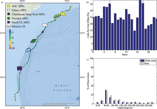
The glider was deployed northeast of Cape Canaveral, Florida, on March 3, 2014, and was recovered southeast of Cape Fear, North Carolina, on April 1, 2014 (Figure 1). The glider was operated near the highly dynamic Gulf Stream, which moves at a higher speed than the glider. Navigation was achieved via modeling of the Gulf Stream’s location and velocity based on glider data and satellite data. The glider’s track traversed several South Atlantic Fishery Management Council MPAs during deployment. The dynamics of the Gulf Stream made some portions of the transit challenging, thus resulting in loops along the glider’s path. The glider first skirted the southeastern corner of the North Florida MPA, approached the Georgia MPA, passed through the Charleston Deep Reef MPA, skirted the southeastern corner of the Edisto MPA, and finally traversed into and out of the western side of the Northern South Carolina (NSC) MPA.

FIGURE 1. Location of autonomous glider deployment off the southeastern U.S. coast in relation to (a) marine protected areas (MPAs; the Northern South Carolina [NSC] MPA, Edisto MPA, Charleston Deep Reef MPA, Georgia MPA, and North Florida [North FL] MPA) and (b) the Gulf Stream. The glider was deployed off Cape Canaveral, Florida, on March 3, 2014, and was recovered off Cape Fear, North Carolina, on April 1, 2014. The red box within the inset in panel (a) illustrates the location of the study area at a broader scale. The black line in both images depicts the location of the glider track.

All acoustic files were analyzed visually and by listening to identify the presence of fish sounds, marine mammal whistles and echolocation, and boat noise. Visual analysis was performed on spectrograms created in MATLAB (MathWorks) using 4,096-point Hanning-windowed fast Fourier transforms (FFTs) with 50% overlap. Due to the frequent occurrence of overlapping calls, both intraspecific and interspecific, each fish sound was documented as either present or absent within an acoustic file, representing a 30-s period. A composite spectrogram was constructed by concatenating a time series of FFTs (100-Hz resolution) from each sound file; this spectrogram illustrated the frequency distribution of sound energy over time. Self-generated glider noise was prevalent across nearly all frequencies. We attempted to remove the influence of such intermittent noise in the composite spectrogram by extracting the median rather than the mean FFT value within each 100-Hz bin.

To calculate the potential detection range of the glider with respect to sound production by the Red Grouper Epinephelus morio (an anticipated focal species), we used a spherical spreading loss model (Urick 1983) and the most intense sound pressure level for this demersal species, which was recorded at 142 dB referenced to (re) 1-μPa root mean square (RMS) in the Gulf of Mexico (GOM; Nelson et al. 2011). Assuming that Red Grouper sounds produced in the GOM do not differ from those produced in Atlantic waters, we used this value as a proxy for source level (SL). The spherical spreading loss model provides a conservative estimate of transmission loss (TL_spherical) for Red Grouper given interactions with the sea floor,

(1)

where R is the range in meters. The signal-to-noise ratio (SNR) was determined as

(2)

where SL is the intensity of a Red Grouper call at 1 m away (estimated as 142 dB re 1-μPa RMS); and NL is the background noise level of the ocean in the 100–200-Hz band. Red Grouper sounds have a peak frequency of 180 Hz; therefore, the 100–200-Hz band represents the main frequency range in which these calls are produced (Nelson et al. 2011; Wall et al. 2014). The NL was calculated from a subset of values that were extracted from the composite spectrogram for periods absent of high noise resulting from anthropogenic or biological sounds. The maximum range in which Red Grouper sounds can be detected given transmission loss and SNR at the source is therefore estimated as

(3)

where R_max is the maximum distance in meters. This model does not account for environmental factors that are known to affect sound transmission, such as depth, bottom type, and temperature profile, and it assumes that humans can detect the presence of a signal in a spectrogram at a 0-dB SNR. Still, it provides a conservative estimate given other studies that have measured fish sound propagation in shallow water (Fine and Lenhardt 1983; Mann and Lobel 1997; Locascio and Mann 2011).

The detection range for marine mammal whistles was also calculated using the same equations and assumptions above and based on an SL of 138 dB re 1 μPa at 1 m, which corresponds to the median SL of common bottlenose dolphins Tursiops truncatus and Atlantic spotted dolphins Stenella frontalis measured in the GOM (Frankel et al. 2014). Based on call characteristics, these two species are the most likely sources of the marine mammal whistles identified in this study (Au and Hastings 2008a). The NL was calculated from the average of a subset of values extracted from the composite spectrogram across 2–10 kHz, the frequency range in which whistles are typically produced, capped by the sample rate of the acoustic recorder (Frankel et al. 2014).

RESULTS

In total, 8,331 files were recorded during the autonomous glider’s mission, which lasted 29 d; the glider traveled 895 km and reached waters 267 m deep. The composite spectrogram illustrates the distribution of sound energy between 0 and 2 kHz recorded over time by the glider (Figure 2). The composite spectrogram was useful for identifying variability in sound levels at different frequencies over time; however, it did not show individual animal sounds. Plots of the glider’s location throughout deployment provided a spatial reference to time stamps marked within the composite spectrogram.

FIGURE 2. Composite spectrogram, showing the band sound pressure level (dB referenced to 1 μPa; 100-Hz resolution) up to 2 kHz, with four date marks (all dates are from 2014; upper panel); and the corresponding position of the autonomous glider along the southeastern U.S. coast on those dates (lower panels). The yellow symbol in the lower panels represents the glider; the direction the icon is facing indicates the glider’s heading. The white flags represent waypoints that were used to navigate the glider during the mission.

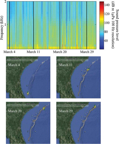
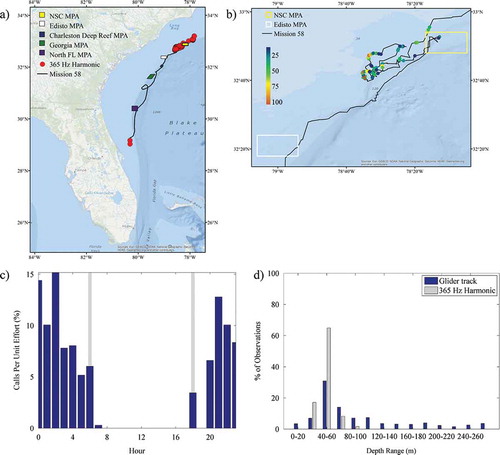
Sounds that were identified throughout the mission included calls from Red Grouper, toadfish Opsanus sp., a 300-Hz FM harmonic (Wall et al. 2012), a 365-Hz harmonic (Wall et al. 2012), marine mammal whistles and echolocation, and noise from vessels. The 300-Hz FM harmonic and 365-Hz harmonic have been previously identified in the GOM; their origin is not known, but they are likely from fish based on their structure and similarity to other fish sounds. See Supplementary Figures S.1–S.5 (available separately online with this article) for example spectrograms of the Red Grouper, 300-Hz FM harmonic, 365-Hz harmonic, marine mammal whistle, and echolocation sounds recorded. The number of files, depth range, and occurrence during the day for these sounds are presented in Table 1. Red Grouper sounds were identified in 120 files (1.44%; Figure 3a). Most of the files (92%; 110 of 120) were recorded in the northern portion of the glider track off North Carolina, with 18% (22 of 120) being observed within the NSC MPA (the only MPA in which Red Grouper sounds were documented; Figure 3b). Red Grouper sound production peaked in the afternoon and lessened between sunset and sunrise (Figure 3c). Over 83% of Red Grouper sound production was observed in waters between 40 and 80 m deep (Figure 3d) within an area where this species has been previously identified in trap surveys (Figure 4). Toadfish calls were rare and were only present off Florida (Figure 5a). The few observations of toadfish occurred in the hours just before sunset (Figure 5b) and in waters of 40–60-m depth (Figure 5c). The 300-Hz FM harmonic sound was observed across a range of depths (Figure 6a), and only 30% (21 of 70) of the detections occurred in the northern portion of the glider track (Figure 6b). Sounds were recorded at night (between sunset and sunrise) as well as in the afternoon (from 1200 to 1600 hours; Figure 6c). Overall, 50% of the 300-Hz FM harmonic sound production was observed in waters of 60–80-m depth (Figure 6d). Only two detections for the 365-Hz FM harmonic occurred off Florida (Figure 7a), while the remaining detections were focused in the shallowest waters within the northern portion of the mission (Figure 7b). The 365-Hz FM harmonic occurred primarily at night (Figure 7c) and in waters 40–60 m deep (Figure 7d).

TABLE 1. Number (N) and percentage of 30-s files that were observed to contain specific sounds; the mean, SD, and range of bottom depths when those sounds were recorded by the autonomous glider; and the percentage of detections that were recorded during daytime hours.

		Depth (m)
Sound	N (%)	Mean ± SD	Range	Daytime detections (%)
Fish
Red Grouper	120 (1.4)	54.2 ± 14.6	38–85.8	70.8
Toadfish Opsanus sp.	4 (0.1)	40.9 ± 0.5	40.6–41.6	100.0
300-Hz FM harmonic	70 (0.8)	71.9 ± 17.5	47.1–137.7	35.7
365-Hz harmonic	373 (4.5)	46.0 ± 9.4	35.6–93.7	0.3
Marine mammals
Whistles	60 (0.7)	77.8 ± 49.2	38.5–241.1	56.7
Echolocation	28 (0.3)	117.9 ± 96.5	34.0–263.0	32.1
Other
Boat	2,151 (25.8)	86.6 ± 56.5	13.9–273.5	45.1

FIGURE 3. (a) Locations of acoustic files that contained Red Grouper sounds across the entire glider track (red circles; N = 120); (b) locations of those same files zoomed in to the northern portion of the track and binned as a percentage of 30-s files per hour; (c) percentage of 30-s files containing Red Grouper sounds normalized by the total number of files that were recorded during each hour (gray bars indicate local sunrise and sunset); and (d) percentage of Red Grouper observations and the overall glider track present within 20-m bottom depth intervals. Site abbreviations used in panels (a) and (b) are defined in Figure 1.

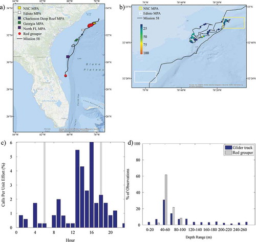
FIGURE 4. Locations of Red Grouper caught in traps (green circles) in southeastern U.S. waters off the South Carolina coast; and locations of Red Grouper sounds recorded by the autonomous glider (red circles). Trap data are from the Southeast Reef Fish Survey (SERFS; see Methods for details).

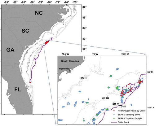
FIGURE 5. (a) Location of acoustic files that contained toadfish sounds across the entire glider track (red circles; N = 4); (b) percentage of 30-s files containing toadfish sound production normalized by the total number of files that were recorded during each hour (gray bars indicate local sunrise and sunset); and (c) percentage of toadfish observations and the overall glider track present within 20-m bottom depth intervals. Site abbreviations used in panel (a) are defined in Figure 1.

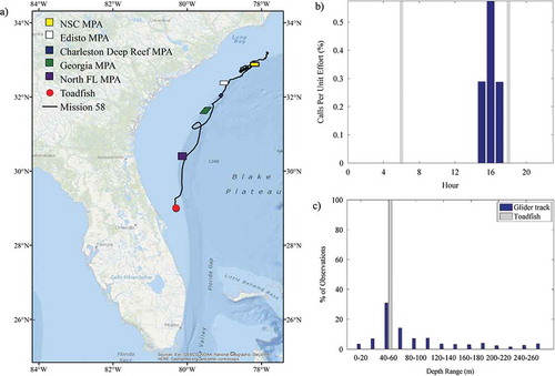
FIGURE 6. (a) Locations of acoustic files that contained 300-Hz FM harmonic sounds across the entire glider track (red circles; N = 70); (b) locations of those same files zoomed in to the northern portion of the track and binned as a percentage of 30-s files per hour; (c) percentage of 30-s files containing 300-Hz FM harmonic sound production normalized by the total number of files that were recorded during each hour (gray bars indicate local sunrise and sunset); and (d) percentage of 300-Hz FM harmonic observations and the overall glider track present within 20-m bottom depth intervals. Site abbreviations used in panels (a) and (b) are defined in Figure 1.

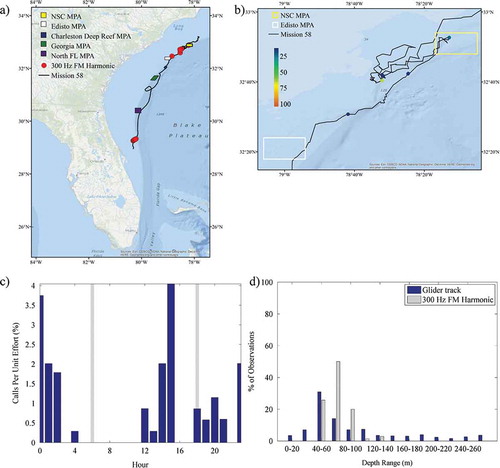
FIGURE 7. (a) Locations of acoustic files that contained 365-Hz harmonic sounds across the entire glider track (red circles; N = 373); (b) locations of those same files zoomed in to the northern portion of the track and binned as a percentage of 30-s files per hour; (c) percentage of 30-s files containing 365-Hz harmonic sound production normalized by the total number of files that were recorded during each hour (gray bars indicate local sunrise and sunset); and (d) percentage of 365-Hz harmonic observations and the overall glider track present within 20-m bottom depth intervals. Site abbreviations used in panels (a) and (b) are defined in Figure 1.

Sounds from marine mammals were also present in the acoustic recordings. Both echolocation and whistles were identified and suspected to be from dolphins, although the species was unknown. Whistles were observed off the coast of Florida, along the shelf slope off the Georgia coast, and in the northern portion of the study area both inside and outside of the NSC MPA (Figure 8a, b). The majority (57%) of whistles were recorded during the day (Figure 8c) and in waters 40–60 m deep (53.3%); however, observations extended into 260-m-deep waters (Figure 8d). Observations of echolocation had a similar spatial extent, although they occurred in water depths greater than 260 m and were primarily observed at night (Figure 9). Figure 10 illustrates the profile of Chl-a and DO along the glider track in relation to the presence of whistles and echolocation. Chl-a blooms were detected by the glider at the start of the deployment and from approximately March 10 to March 14; these periods corresponded to observations of whistles and echolocation. Biofouling severely affected the sensor after March 29, as illustrated by the sudden and consistent elevation of Chl-a values throughout the water column. The true Chl-a beyond that time was unknown. Biofouling may have affected the reported Chl-a as early as March 20, evidenced by a steadier though less-consistent elevation of values; however, the extent of the impact is unknown. Noise from vessels was prevalent throughout the mission, with the highest concentrations observed off Florida and north of the Edisto MPA (Figure 11a). Vessel noise was present during all hours of the day, peaking slightly at sunrise and sunset (Figure 11b), and in all depth ranges of the glider track (Figure 11c).

FIGURE 8. (a) Locations of acoustic files that contained marine mammal whistle sounds across the entire glider track (red circles; N = 60); (b) locations of those same files zoomed in to the northern portion of the track and binned as a percentage of 30-s files per hour; (c) percentage of 30-s files containing marine mammal whistles normalized by the total number of files that were recorded during each hour (gray bars indicate local sunrise and sunset); and (d) percentage of whistle observations and the overall glider track present within 20-m bottom depth intervals. Site abbreviations used in panels (a) and (b) are defined in Figure 1.

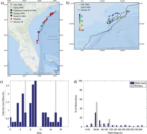
FIGURE 9. (a) Locations of acoustic files that contained marine mammal echolocation sounds across the entire glider track (red circles; N = 28); (b) locations of those same files zoomed in to the northern portion of the track and binned as a percentage of 30-s files per hour; (c) percentage of 30-s files containing marine mammal echolocation sounds normalized by the total number of files that were recorded during each hour (gray bars indicate local sunrise and sunset); and (d) percentage of echolocation observations and the overall glider track present within 20-m bottom depth intervals. Site abbreviations used in panels (a) and (b) are defined in Figure 1.

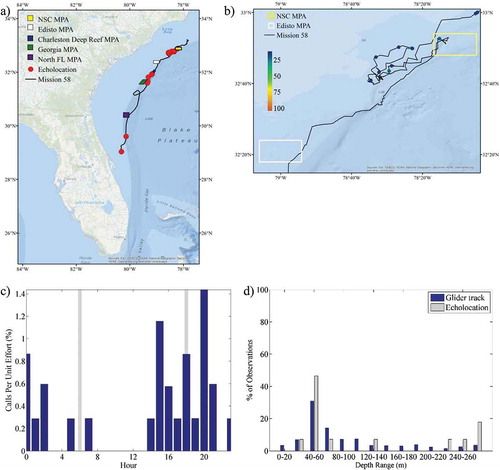
FIGURE 10. Glider-derived chlorophyll-a concentration (µg/L; log scale; upper panel) and dissolved oxygen concentration (mg/L; lower panel) off the southeastern U.S. coast over time. The plots are overlaid with observations of marine mammal whistles (black shaded circles) and echolocation sounds (open squares) displayed at the glider’s depth at the time the sounds were recorded.

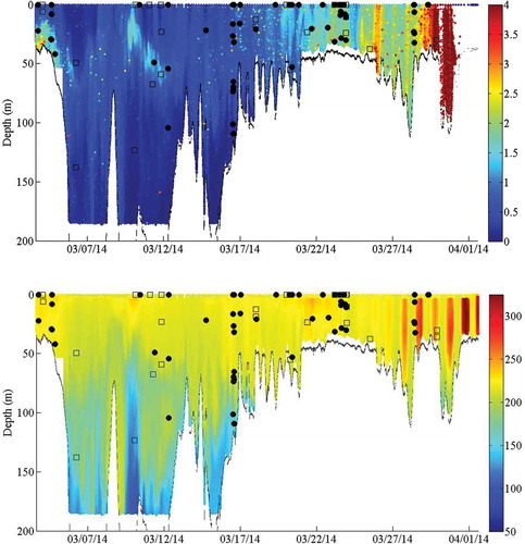
FIGURE 11. (a) Locations of acoustic files that contained boat noise across the entire glider track binned as a percentage of 30-s files per hour (N = 2,151); (b) the percentage of 30-s files containing boat noise normalized by the total number of files that were recorded during each hour (gray bars indicate local sunrise and sunset); and (c) percentage of boat noise and the overall glider track observations present within 20-m bottom depth intervals. Site abbreviations used in panel (a) are defined in Figure 1.

The mean NL extracted from the composite spectrogram within the 100–200-Hz bin was 85.8 dB re 1 μPa, with an SD of 4.9 dB (N = 20). Therefore, the SNR at the source, assuming a Red Grouper signal of 142 dB re 1 μPa, was 50.2 dB. This resulted in an R_max of 645 m for Red Grouper sound production, on average, assuming spherical spreading. The mean NL extracted from the composite spectrogram across 2–10 kHz was 65.9 dB re 1 μPa, with an SD of 6.8 dB (N = 100); an R_max of 4 km for dolphin whistles was calculated.

DISCUSSION

This research demonstrated the potential utility of passive acoustic recording onboard an autonomous glider for generating results to determine fish, marine mammal, and boat distributions, all of which are important for fisheries management, protected species management, and marine spatial planning. To our knowledge, this is the first demonstration of ocean glider deployment in the Gulf Stream, including establishing the glider’s ability (at times limited) to enter and exit the current to control its location. Through these efforts, we identified a variety of sounds in the acoustic recordings, namely sounds from Red Grouper and toadfish; two sounds (putatively originating from fish) that were previously documented in the GOM; whistles and echolocation from marine mammals; and extensive noise from vessel traffic. Numerous sounds from previously undocumented sources were also observed (data not shown).

For all species except toadfish and the 300-Hz harmonic, the majority of sound production (accounting for sampling effort) was detected in continental shelf waters off the coasts of Georgia and South Carolina as opposed to shelf-break or upper-slope waters. Most of the toadfish and 300-Hz sounds were detected on the Florida shelf early in the glider’s deployment period; this result is depicted in the composite spectrogram as an increase in amplitude (i.e., noise) when the glider reached the northern portion of the glider track around March 13. Prior to that, from approximately March 5 to March 12, a period of relatively low amplitude (i.e., quiet) was recorded. This time frame corresponded to when the glider traveled up the Gulf Stream along the deep waters of the continental shelf, suggesting that fish sound production may be reduced in continental shelf-break and upper-slope waters. As the glider traversed the entire water column from near the surface to 185-m depth at an average rate of 45–50 min/cycle, pelagic and demersal sound producers would likely have been recorded when the glider was nearby. The quiet period from March 5 to March 12 was aided by the lack of vessel noise observed in the same region.

The Red Grouper was the only serranid that was frequently recorded during the glider mission, and Red Grouper sounds were documented throughout the day and night. Although the glider traversed a large area with varying depths (continental shelf to upper slope), Red Grouper sound production was predominantly documented in continental shelf and (to a lesser extent) shelf-break waters. This region and the observed characteristics of Red Grouper sound production are consistent with results from research conducted in the eastern GOM, during which sounds were observed in continental shelf waters throughout a 24-h period, with decreased calling between sunset and sunrise (Nelson et al. 2011; Wall et al. 2014). These results suggest that hydrophone-equipped gliders could be used to survey Red Grouper distributions in SEUS continental shelf waters.

In the eastern GOM between 4- and 984-m bottom depths, the 300-Hz FM harmonic sounds were found in waters of about 50–200-m depth, whereas the 365-Hz harmonic sounds were most common in depths shallower than 40 m (Wall et al. 2013). These depth ranges are consistent with those observed for the 365-Hz harmonic and 300-Hz FM harmonic sounds in the present study. Notably, however, the 300-Hz FM harmonic sound was recorded during both diurnal and nocturnal hours in this study, whereas it was limited to nocturnal hours in the GOM (Wall et al. 2013). The reason for this regional difference is unknown. We hypothesize that these sounds may be produced by Northern Sea Robins Prionotus carolinus (365 Hz) and Atlantic Midshipmen Porichthys plectrodon (300 Hz), since both species are found in the GOM and Atlantic Ocean. Further investigation into the source of the 300-Hz FM harmonic sound—namely whether different species are responsible for the varying sound characteristics—is needed. In fact, we detected a wealth of previously undocumented sounds that we suspected were produced by fish (data not shown), thus highlighting the dearth in our current knowledge of the sources and characteristics of fish-generated sounds. A greater understanding of communication in all soniferous fish species could greatly benefit fishery-independent monitoring efforts and facilitate studies to assess distributional ranges and variations in behavior.

Marine mammal sounds were the only biological sounds observed in waters beyond 140-m depth. Echolocation was more common at night and was detected in deeper waters than whistles. The exact location of the sounds’ source in the water column was unknown, so it was impossible to correlate the observed sounds to depth-specific oceanographic data. However, the occurrence and frequency of both whistles and echolocation clicks appeared to coincide with subsurface Chl-a blooms in the water column and along the shelf slope, thus suggesting an association with feeding behavior and consistent with the use of echolocation at depth to find and identify prey (Au and Hastings 2008b).

Noise from vessel traffic was ubiquitous throughout the glider mission, during which 25% of the files contained boat noise. In comparison, only about 1.5% (403 of 25,129 files) of the files from glider-based research in the GOM contained boat noise (Wall et al. 2013). The potential degree to which biological sounds were masked by vessel noise likely varied from minimal (distant, low-amplitude, low-frequency single tones) to high (high-amplitude, numerous tones ranging across all frequencies). Vessel noise was most frequently and consistently observed during sunrise and sunset; thus, there was a high potential for the masking of biological sounds during those periods. Quantifying the extent to which boat noise impacted communication for the observed marine organisms was outside the scope of this study. However, research has shown that anthropogenic noise imposes deleterious effects on the behavior of both fishes and marine mammals (Popper et al. 2003; Nowacek et al. 2007; Slabbekoorn et al. 2010; Hatch et al. 2012). Additionally, high-amplitude broadband noise associated with vessel traffic could significantly reduce the detection range of biological sounds. Hydrophone-equipped glider surveys for mapping the distributions of Red Grouper, other fishes, or marine mammals must take this issue into account.

To our knowledge, we have demonstrated the first use of an ocean glider to perform extensive surveys in Gulf Stream and adjacent waters, including the glider’s ability—albeit limited at times—to enter and exit the current to control location and trajectory based on real-time ocean model predictions. Results indicated the potential utility of a glider-based passive acoustic approach to assessing fish, marine mammal, and boat distributions. These findings are relevant for fisheries management, protected species management, and marine spatial planning, especially given the likelihood of increased anthropogenic noise from such sources as shipping traffic and energy exploration surveys in the U.S. Atlantic planning area of the continental shelf (BOEM 2015). One disadvantage of sampling with gliders is the spatiotemporal component that confounds the data sets. Because the glider moves as it collects data, the separation of temporal variability (e.g., day–night variation) from spatial variability is difficult. Such confounding of the data can be addressed by (1) using fixed passive acoustic recording stations to assess temporal variability and (2) constraining analyses to the known sound production periods for the species of interest. For example, when fish species are known to make sound predominately at night, only glider-sampled data from nighttime should be used to indicate species presence or absence. Advanced sampling technologies with broad, multiple-region applicability can fill gaps in information on the distribution of soniferous species and can guide the implementation of additional survey techniques (e.g., active acoustic mapping efforts and video or visual surveys) to ground-truth species identification, develop “sound-to-abundance” conversion capabilities, and identify environmental and geomorphological characteristics associated with acoustic hot spots and likely spawning aggregation sites.

ACKNOWLEDGMENTS

Trap data presented in Figure 4 were primarily collected by the Marine Resources Monitoring, Assessment, and Prediction Program (SCDNR) and by the Southeast Area Monitoring and Assessment Program–South Atlantic. This study was funded by the Advanced Sampling Technology Working Group of the NOAA NMFS. Publication of this article was funded by the University of Colorado Boulder Libraries Open Access Fund.

REFERENCES

- Au, W. W. L., and M. C. Hastings. 2008a. Principles of marine bioacoustics. Springer, New York.
- Au, W. W. L., and M. C. Hastings. 2008b. Echolocation in marine mammals. Pages 501–564 in W. W. L. Au and M. C. Hastings, editors. Principles of marine bioacoustics. Springer, New York.
- Bacheler, N. M., C. M. Schobernd, Z. H. Schobernd, W. A. Mitchell, D. J. Berrane, G. T. Kellison, and M. J. Reichert. 2013. Comparison of trap and underwater video gears for indexing reef fish presence and abundance in the southeast United States. Fisheries Research 143:81–88.
- Baumgartner, M. F., D. M. Fratantoni, T. P. Hurst, M. W. Brown, T. V. Cole, S. M. Van Parijs, and M. Johnson. 2013. Real-time reporting of baleen whale passive acoustic detections from ocean gliders. Journal of the Acoustical Society of America 134:1814–1823.
- Bingham, B., N. Kraus, B. Howe, L. Freitag, K. Ball, P. Koski, and E. Gallimore. 2012. Passive and active acoustics using an autonomous wave glider. Journal of Field Robotics 29:911–923.
- BOEM (Bureau of Ocean Energy Management). 2015. Atlantic geological and geophysical (G&G) activities programmatic environmental impact statement (PEIS). Available: http://www.boem.gov/Atlantic-G-G-PEIS/. ( December 2015).
- Coleman, F. C., C. C. Koenig, G. R. Huntsman, J. A. Musick, A. M. Eklund, J. C. McGovern, G. R. Sedberry, R. W. Chapman, and C. B. Grimes. 2000. Long-lived reef fishes: the grouper–snapper complex. Fisheries 25(3):14–21.
- Fine, M. L., and M. L. Lenhardt. 1983. Shallow-water propagation of the Toadfish mating call. Comparative Biochemistry and Physiology Part A: Physiology 76:225–231.
- Frankel, A. S., D. Zeddies, P. Simard, and D. Mann. 2014. Whistle source levels of free-ranging bottlenose dolphins and Atlantic spotted dolphins in the Gulf of Mexico. Journal of the Acoustical Society of America 135:1624–1631.
- Gell, F., and C. Roberts. 2002. The fishery effects of marine reserves and fishery closures. World Wildlife Fund, Washington, D.C.
- Hatch, L. T., C. W. Clark, S. M. Van Parijs, A. S. Frankel, and D. W. Ponirakis. 2012. Quantifying loss of acoustic communication space for right whales in and around a U.S. national marine sanctuary. Conservation Biology 26:983–994.
- Hyun, K. H., and R. He. 2010. Coastal upwelling in the South Atlantic Bight: a revisit of the 2003 cold event using long-term observations and model hindcast solutions. Journal of Marine Systems 83:1–13.
- Locascio, J. V., and D. A. Mann. 2011. Localization and source level estimates of Black Drum (Pogonias cromis) calls. Journal of the Acoustical Society of America 130:1868–1879.
- Mann, D. A., and P. S. Lobel. 1997. Propagation of damselfish (Pomacentridae) courtship sounds. Journal of the Acoustical Society of America 101:3783–3791.
- Matsumoto, H., J. H. Haxel, R. P. Dziak, D. R. Bohnenstiehl, and R. W. Embley. 2011. Mapping the sound field of an erupting submarine volcano using an acoustic glider. Journal of the Acoustical Society of America 129:EL94–EL99.
- Nelson, M., C. C. Koenig, F. C. Coleman, and D. A. Mann. 2011. Sound production by Red Grouper (Epinephelus morio) on the west Florida shelf. Aquatic Biology 12:97–108.
- Nowacek, D. P., L. H. Thorne, D. W. Johnston, and P. L. Tyack. 2007. Responses of cetaceans to anthropogenic noise. Mammal Review 37:81–115.
- Popper, A. N., J. Fewtrell, M. E. Smith, and R. D. McCauley. 2003. Anthropogenic sound: effects on the behavior and physiology of fishes. Marine Technology Society Journal 37:35–40.
- Rudnick, D. L., R. E. Davis, C. C. Eriksen, D. M. Fratantoni, and M. J. Perry. 2004. Underwater gliders for ocean research. Marine Technology Society Journal 38:73–84.
- SAFMC (South Atlantic Fishery Management Council). 2015a. Snapper grouper. Available: http://safmc.net/useful-info/snapper-grouper/. ( December 2015).
- SAFMC (South Atlantic Fishery Management Council). 2015b. Snapper grouper management complex: species managed by the South Atlantic Fishery Management Council. Available: http://safmc.net/Library/pdf/SAFMC_SnapperGrouperManagedSpecies_12182012.pdf. ( December 2015).
- Schofield, O., J. Kohut, D. Aragon, L. Creed, J. Graver, C. Haldeman, J. Kerfoot, H. Roarty, C. Jones, and D. Webb. 2007. Slocum gliders: robust and ready. Journal of Field Robotics 24:473–485.
- Slabbekoorn, H., N. Bouton, I. Van Opzeeland, A. Coers, C. Ten Cate, and A. N. Popper. 2010. A noisy spring: the impact of globally rising underwater sound levels on fish. Trends in Ecology and Evolution 25:419–427.
- Urick, R. 1983. Principles of underwater sound. McGraw-Hill, New York.
- Wall, C. C., C. Lembke, and D. A. Mann. 2012. Shelf-scale mapping of sound production by fishes in the eastern Gulf of Mexico using autonomous glider technology. Marine Ecology Progress Series 449:55–64.
- Wall, C. C., P. Simard, C. Lembke, and D. A. Mann. 2013. Large-scale passive acoustic monitoring of fish sound production on the west Florida shelf. Marine Ecology Progress Series 484:173–188.
- Wall, C. C., P. Simard, M. Lindemuth, C. Lembke, D. F. Naar, C. Hu, B. B. Barnes, F. E. Muller-Karger, and D. A. Mann. 2014. Temporal and spatial mapping of Red Grouper Epinephelus morio sound production. Journal of Fish Biology 85:1469–1487.
- Xue, Z., J. Zambon, Z. Yao, Y. Liu, and R. He. 2015. An integrated ocean circulation, wave, atmosphere and marine ecosystem prediction system for the South Atlantic Bight and Gulf of Mexico. Journal of Operational Oceanography 8:80–91.
- Zhao, J., C. Hu, J. M. Lenes, R. H. Weisberg, C. Lembke, D. English, J. Wolny, L. Zheng, J. J. Walsh, and G. Kirkpatrick. 2013. Three-dimensional structure of a Karenia brevis bloom: observations from gliders, satellites, and field measurements. Harmful Algae 29:22–30.