Prediction analysis of landslide displacement trajectory based on the gradient descent method with multisource remote sensing observations

Abstract

Landslides can result in extensive casualties and huge economic losses. The accurate discrimination of the main slip direction and deformation trajectory is an important prerequisite for studying landslide formation mechanisms and designing landslide control schemes. In the process of landslide evolution over time, the main slip direction also changes dynamically and provides a comprehensive reflection of the landslide displacement state. However, few studies on this topic have been published. In this paper, a new methodology for analyzing slope stability is proposed based on three techniques: interferometric synthetic aperture radar (InSAR), unmanned aerial vehicle (UAV), and ground-based interferometric synthetic aperture radar (GB-InSAR). The Small Baseline Subset Interferometric SAR (SBAS-InSAR) technique is combined with an overall analysis of the study area to identify the regions of interest (ROIs) with large deformation and the starting target points, and the fusion results of radar deformation data (RDD) and digital surface model (DSM) data are used to fit the deformation surface field of the ROIs. The gradient descent approach is executed to obtain the running trajectory points of the target masses so that the main slip direction and displacement trajectory in the study area can be predicted at small scales. The measured data for the Hongshiyan landslide in Yunnan Province are used to verify the effectiveness of the method, and the predicted results are consistent with the actual landslide direction. The experimental results show that the method can exactly identify the deformation area, especially in the case of a fast-changing deformation trend. This approach can provide more accurate monitoring area results to support the rapid control and prevention of landslide hazards by analyzing the minimum pixel grid (i.e. points), as the smallest spatial unit at a time interval of minutes. The study shows that the method can efficiently combine space–Earth multisource monitoring data to clarify the main slide direction and improve the postslide trajectory prediction of the slope, which is beneficial for assessing disaster risks and improving landslide prevention and control effects, reflecting the engineering application value of the approach.

Keywords:

• main slip direction
• deformation trajectory
• slope stability
• space–earth multisource monitoring data
• landslide monitoring

1. Introduction

Landslides are a common type of geohazard worldwide. In mountainous areas, the large scale and fast speed of landslides can destroy villages, kill people, damage roads, and even block rivers, leading to heavy casualties and considerable economic losses (Ehteshami-Moinabadi and Nasiri 2019; Kumar et al. 2019; Lacroix et al. 2020). China is a nation with frequent landslide disasters and giant landslides, which account for most of the damage (Hong et al. 2017; Qiu et al. 2017; Dai et al. 2019). According to the National Geological Disaster Bulletin 2020, there were 7,840 geological disasters in 2020, including 4,810 landslides, accounting for 61.35% of the total number of geological disasters. The number of geological disasters increased by 26.8% compared to that in 2019, posing a great threat to lives and property (Liu and Chen 2020).

Over the years, with the rapid development of sensors, Internet of Things technology, and multidisciplinary integration, China and other nations have strengthened geological disaster prevention and control cooperation; several effective and efficient systems have been formed, including investigation and assessment systems, monitoring and early warning systems, comprehensive management systems, and emergency prevention systems (Alamdar et al. 2015; Dong et al. 2018; Intrieri et al. 2018; Carla et al. 2019; Dai et al. 2020; Li et al. 2020; Solari et al. 2020; Xu et al. 2020; Yu et al. 2021; Zhang et al. 2021). Synthetic aperture radar interferometry (InSAR) provides a new tool to study geohazards and survey topography (Casagli et al. 2010; Mazzanti 2011; Lazecky et al. 2015; Di Matteo et al. 2017). While the question of where a potential landslide hazard will occur is the precondition for further study, the sliding direction, trajectory, and hazard range are the focus of landslide assessment. Combining the early identification of landslides with sliding direction and sliding trajectory prediction for later landslide stability analysis, landslide hazard prediction, and early warning and prevention plan design work can effectively eliminate or reduce the risk of damage caused by landslide disasters.

Landslide movement trajectory monitoring is very important to landslide monitoring and early warning, and the main slide direction and displacement trajectory of a landslide are often indicative in specific circumstances of where a landslide disaster might occur and the impact of the disaster after it has occurred (Kawamura et al. 2007). Determining the sliding surface of a landslide is a difficult task because each landslide is usually a complex combination of many small movements. A great number of different approaches, which can be roughly classified into two categories, have been used to solve this problem: 1. the theoretical solution of the main sliding direction is obtained by deriving the formula of the corresponding main slide direction based on empirical and semiempirical methods assuming certain conditions; 2. dynamic prediction is performed to discern the main sliding direction based on the data obtained by the current monitoring technology.

In recent years, the semiempirical method of determining the direction of landslides by on-site geological surveys and geomorphological feature analysis has been the most common approach to determining the direction of landslides (Dong et al. 2009; Segoni et al. 2018; Tian et al. 2020). The sliding direction of the slope is mainly determined with an empirical or semiempirical approach, e.g. the whole vector direction of the displacements monitored inside the slope and/or a hypothesis developed based on the displacement parallel to the bottom of the potential slip surface or the failure mechanism of the slope (Liu et al. 2018; Chen et al. 2021). A simple monitoring method for the early warning of rainfall-induced landslides is proposed. Tilting angles in the surface layer of the slope are mainly monitored in this method (Uchimura et al. 2010; 2015; Dikshit and Satyam 2019). However, the traditional empirical method is susceptible to human factors and lacks an accurate quantitative basis, which can have an impact on the results of a series of later landslide calculations. Moreover, it is difficult to give an exact direction of the main slide for complex slopes via this approach. During the last decade, considerable progress has been made in applying the deformation monitoring technique to detect ground movements and forecast landslides. Some scholars have also applied information from contact monitoring results, such as multipoint displacement gauges and borehole inclinometers, to obtain the vector curve of the combined displacement in the plane over a given time, thus revealing the unique deformation characteristics of the excavated slope and the main slide direction of the landslide under special geological conditions (Zhang et al. 2005; Dong et al. 2016; Chung and Lin 2019). Based on advanced remote sensing technology, Liao Bin et al. studied the Beidou communication landslide monitoring system with the addition of displacement sensors, while Li Qun et al. used a monitoring instrumentation system composed of GPS and other components to perform dynamic discrimination of the main slide direction (Liao and Wang 2014; Li et al. 2019; Nie et al. 2019). However, the method of using a single-point deformation monitoring network is extremely demanding in terms of terrain and engineering volume in the placement of monitoring stations, making it difficult to achieve high-density coverage of the entire monitoring area (Wang et al. 2005; Yin et al. 2010; Benoit et al. 2015). It is imprecise to identify the main sliding direction of landslides via limited monitoring data because these limited are insufficient data for precisely reflecting the actual movement and deformation of landslides.

Therefore, there is an urgent need for a method for predicting the main sliding direction and sliding trajectory of slopes to achieve rapid control and prevention of landslide hazards. The main slip direction of a landslide is a comprehensive reflection of the displacement state of the landslide, which can either represent the overall sliding direction of the entire landslide or determine the movement and direction of the slide. The accurate identification of the main landslide direction is an important basis for studying the formation mechanism of landslides, carrying out stability evaluation, and designing prevention and control plans. In geographic analysis, we frequently see studies that use similarity in geographic environments or areas to assess the similarity of other geographic variables or activities at other locations or areas. In this study, the deformation areas of interest in the study area are roughly determined by using satellite-based SAR, and then the information from the ground-based radar monitoring sites is used to fuse the topographic information to construct a deformation field fitting model and determine the sliding direction of each area of the slope. A method is proposed to fit the deformation field of the neighborhood near the target mass, to obtain running track points based on the gradient of the fitted surface at the target mass and to derive the probable main slide direction of the landslide at the next moment by integrating the current slide direction and topographic changes. Our approach initially employed the large-scale surface monitoring data obtained by ground-based radar to overcome the limitations of traditional main-slip direction prediction and improve the rapid control and prevention of landslide hazards under the influence of gravity.

2. Materials and methods

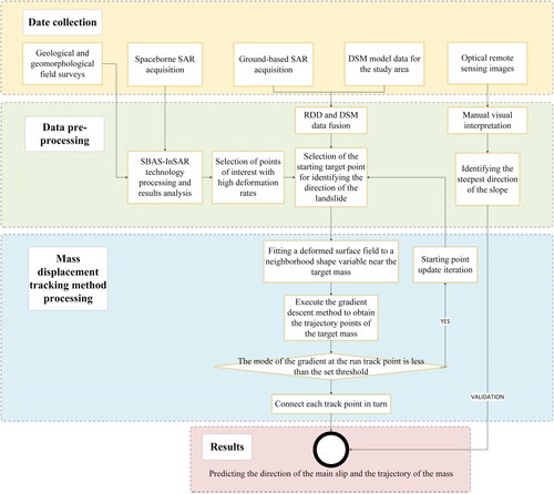
2.1. Data-processing flow

This study proposes a real-time tracking method for slope displacement monitoring based on the large-range surface monitoring capability of spaceborne SAR and ground-based SAR, combined with UAV terrain data, to predict the landslide main slip direction and postslip displacement trajectory (the data processing flow is shown in Figure 1). First, radar deformation data (RDD) and UAV digital surface model (DSM) data are acquired and fused to unify the resolution of the two datasets and to include geographic information in the deformation data. Second, pixel points with higher deformation rates are obtained from the SBAS-InSAR results in the study area as the starting point for identifying the main slip direction. Finally, the gradient of the deformation field at the target mass is calculated, and the gradient descent method is employed to obtain the trajectory points of the target mass. The result of the data fusion is the current main landslide direction, while the result of the topographic data analysis is the direction of the steepest slope. The probable main sliding direction of the landslide at the next moment can be derived by combining the current direction of sliding and changes in topography. The problem of changes in the main slip direction of the deformation in different areas during traditional slope deformation monitoring is solved by fitting a second-order surface to the deformation variables in the neighborhood of the target mass and obtaining the running track points according to the gradient of the fitted surface at the target mass. Accordingly, utilization of the real-time tracking of slope mass displacement deformation monitoring improves the accuracy and efficiency of the monitoring.

Figure 1. Flow chart of the method for predicting the direction and trajectory of the main slide in a landslide subregion.

2.2. Time series analysis with SBAS-InSAR

At present, because InSAR technology is not restricted by weather and has the advantages of large-scale and high-precision monitoring, it has been widely used in the identification of geological disasters (Raspini et al. 2017; Li et al. 2019; Xue et al. 2020). In particular, SBAS-InSAR technology eliminates the limitations of time and space incoherence and atmospheric effects in traditional interferometry methods, making the deformation results more continuous in time and space. This technology has been widely used for studies of surface subsidence, earthquakes, volcanoes, active faults, frozen soil deformation, and glacier movement to identify unstable slopes subjected to creep and landslides (Euillades et al. 2016; Le et al. 2016; Zhou et al. 2017; Chen et al. 2018; Lin et al. 2019; Shih et al. 2019). First, the SBAS-InSAR technique generates an appropriate combination of differential interferograms produced by SAR data pairs based on baseline threshold values. Second, this technique estimates the deformation information of every single differential interferogram and regards them as observed values. Finally, SBAS-InSAR retrieves the deformation rate and time series based on the observed values acquired in the previous step. The results are based on the following equations:

Assuming that $N+1$ SAR images were acquired for the same region at regular times ($t_0,\dots ,t_N$), $M$ differential interferograms can be generated. The inequality of $M$ is defined as follows: (1) $$\frac{N+1}{2}\le M\le \frac{N(N+1)}{2}$$(1)

For the differential interferogram $j$ generated from the images acquired at $t_A$ and $t_B$ ($t_A{<t}_B$), the phase of any point $(x,r)$ is as follows: (2) $$\mathrm{\delta }{\mathrm{\varphi }}_j\left(\mathrm{x},\mathrm{ }\mathrm{r}\right)=\mathrm{\varphi }\left({\mathrm{t}}_{\mathrm{B}},\mathrm{ }\mathrm{x},\mathrm{ }\mathrm{r}\right)-\mathrm{\varphi }\left({\mathrm{t}}_{\mathrm{A}},\mathrm{ }\mathrm{x},\mathrm{ }\mathrm{r}\right)\text{ ≈ Δ}{\mathrm{\varphi }}_{\text{disp}}+\mathrm{\Delta }{\mathrm{\varphi }}_{\text{topo}}+\mathrm{\Delta }{\mathrm{\varphi }}_{\text{orb}}+\mathrm{\Delta }{\mathrm{\varphi }}_{\text{atm}}+\mathrm{\Delta }{\mathrm{\varphi }}_{\text{noise}}$$(2) where $\mathrm{\varphi }\left({\mathrm{t}}_{\mathrm{B}},\mathrm{ }\mathrm{x},\mathrm{ }\mathrm{r}\right)$ and $\mathrm{\varphi }\left({\mathrm{t}}_{\mathrm{A}},\mathrm{ }\mathrm{x},\mathrm{ }\mathrm{r}\right)$ are the phases of the two images at point $\left(\mathrm{x},\mathrm{ }\mathrm{r}\right);$ $\mathrm{\Delta }{\mathrm{\varphi }}_{\text{disp}}$ is the phase formed by the cumulative deformation of the line of sight (LOS) at ${\mathrm{t}}_{\mathrm{B}}$ and ${\mathrm{t}}_{\mathrm{A}}$ relative to ${\mathrm{t}}_0;$ and the phase errors caused by topography, orbit, atmosphere, and noise are represented by $\mathrm{\Delta }{\mathrm{\varphi }}_{\text{topo}},\mathrm{ }\mathrm{\Delta }{\mathrm{\varphi }}_{\text{orb}},\mathrm{ }\mathrm{\Delta }{\mathrm{\varphi }}_{\text{atm}},\mathrm{ }\text{and}\mathrm{ }\mathrm{\Delta }{\mathrm{\varphi }}_{\text{noise}},$ respectively. SBAS-InSAR removes the residual components from the interferometric phase to obtain the deformation phase $\mathrm{\Delta }{\mathrm{\varphi }}_{\text{disp}}.$ Then, a system of $M$ equations with $N$ unknowns can be organized as the following matrix: (3) $$A\varphi =\delta \varphi$$(3) where A corresponds to an $M \times N$ coefficient matrix and $\forall j = 1, \cdots \mathrm{, }M.$ M and N represent the numbers of interferograms and SAR acquisitions, respectively. ${\varphi }^T = [\phi (t_1), \cdots , \phi (t_N)]$ denotes the vector of unknown phase values related to high-coherence pixels. $\delta {\varphi }^T = [\delta {\varphi }_1, \cdots , \delta {\varphi }_N]$ represents the vector of unwrapped phase values associated with differential interferograms. The deformation velocity can be obtained by rewriting Equation (3)(3) $$A\varphi =\delta \varphi$$(3) into the following equation: (4) $$Bv=\delta \varphi$$(4) where $B$ represents an $M\times N$ coefficient matrix, and $v^T$ can be expressed as follows: (5) $$v^T=\left[v_1=\frac{{\varphi }_1}{t_1-t_0},\dots ,v_N=\frac{{\varphi }_N-{\varphi }_{N-1}}{t_N-t_{N-1}}\right]$$(5)

Finally, the least squares (LS) or singular value decomposition (SVD) algorithms can be applied to Equations (4)(4) $$Bv=\delta \varphi$$(4) and (5)(5) $$v^T=\left[v_1=\frac{{\varphi }_1}{t_1-t_0},\dots ,v_N=\frac{{\varphi }_N-{\varphi }_{N-1}}{t_N-t_{N-1}}\right]$$(5) to calculate the deformation velocity. The cumulative deformation can be generated by performing the calculation on the aforementioned equations over a specific time span (Lu et al. 2020; Cigna and Tapete 2021).

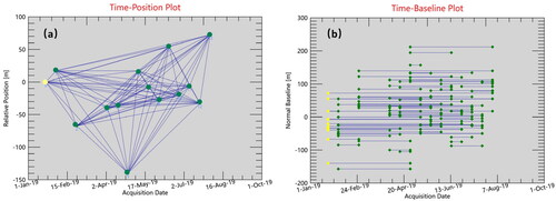
As shown in Figure 2, the image acquired on 1 January 2019 (yellow point) was selected as the supermaster image for the interferometric combinations, and all slave images were coregistered and resampled to the supermaster image. According to the climate and vegetation cover conditions of the study area, the spatial baseline and temporal baseline were set at 5% and 200, respectively, the space baseline used in the analysis was 105 meters, and the longest temporal baseline was 192 days. Then, the Goldstein filter and 2 D unwrapping method were used for interferometric processing, and the unwrapping threshold was set to 0.35. Subsequently, 11 interferometric pairs with poor coherence were deleted, while 91 interferometric pairs were used in subsequent time-series analysis. In the nondeformation region, 66 ground control points were selected for refinement by Andre flattening, and the control points were screened to ensure that there were sufficient control points and that the deviation was within 1.5. In the first inversion, we selected the linear model to estimate the surface deformation rate and residual topography. Ground control points were introduced in the second inversion to eliminate atmospheric phase interference and obtain a more accurate time-series displacement. Finally, geocoding was performed to obtain the average deformation velocity and displacement of the study area in the direction of the radar LOS.

Figure 2. (a) Time–position of Sentinel-1A image interferometric pairs; (b) time–baseline of Sentinel-1A image interferometric pairs. (The yellow point denotes the supermaster image. Blue lines represent interferometric pairs. Green diamonds denote slave images.).

2.3. Establishment of the 3 D surface field

When the SAR system works on a ground-based platform, its observational topology is as shown in Figure 3(a). The microvariable monitoring radar uses synthetic aperture radar imaging to achieve long-range 2 D imaging of a large area, with the result being a projection of the actual scene onto the imaging plane, as shown in Figure 3(b).

Figure 3. Schematic diagram of RDD and DSM data fusion. (a) 3 D model of the GB-InSAR system observation geometry; (b) GB-InSAR plane geometry model in a range–azimuth coordinate system.

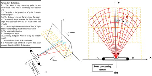
First, the DSM data of the slope are obtained by using the UAV tilt photogrammetry technique $\left(x,y,h\right),$ which is the corresponding geographic coordinate value of the selected coordinate system. The 3 D laser scanner scans the GB-InSAR device for coordinate positioning to obtain the coordinates of the two endpoints $\mathrm{A}\left(x_A,y_A,z_A\right)$ and $\mathrm{B}\left(x_B,y_B,z_B\right)$ of the system guideway in the same geographic coordinate system as the UAV. It is reasonable to assume that the center of the radar trajectory is the coordinate origin $\mathrm{O},$ the distance direction is the $\mathrm{X}$ direction, the azimuth direction is the $\mathrm{Y}$ direction (direction of radar movement) and the altitude direction is the $\mathrm{Z}$ direction (Jia et al. 2016).where the average of the two endpoint coordinates is taken as the radar antenna phase center coordinates O $\left(x_o,y_o,z_o\right):$ (6) $$x_o=\frac{x_A+x_B}{2}$$(6) (7) $$y_o=\frac{y_A+y_B}{2}$$(7) (8) $$z_o=\frac{z_A+z_B}{2}$$(8) where P $\left(x_P,y_P,z_P\right)$ is any scattering point in the observation scene with a scattering cross-section of $\sigma \left(x,y\right).$ Then, the echo signal of the radar for a given target P can be calculated as follows: (9) $$S_P\left(K_{\omega },y\right)=\sqrt{\sigma \left(x,y\right)}\frac{\exp \hspace{0.17em}\left(-j{K}_{\omega }{R}_T\right)}{{R_T}^2}$$(9)

In Equation (9)(9) $$S_P\left(K_{\omega },y\right)=\sqrt{\sigma \left(x,y\right)}\frac{\exp \hspace{0.17em}\left(-j{K}_{\omega }{R}_T\right)}{{R_T}^2}$$(9) , $K_{\omega }$ is the spatial frequency of the signal, and $R_T$ is the distance from the radar to the target P. For the observed scenario, the radar receives the echo signal using the following equation: (10) $$S_P\left(K_{\omega },y\right)={\iint }_W\sqrt{\sigma \left(x,y\right)}\frac{\exp \hspace{0.17em}\left(-j{K}_{\omega }{R}_T\right)}{{R_T}^2}dr$$(10)

In Equation (10)(10) $$S_P\left(K_{\omega },y\right)={\iint }_W\sqrt{\sigma \left(x,y\right)}\frac{\exp \hspace{0.17em}\left(-j{K}_{\omega }{R}_T\right)}{{R_T}^2}dr$$(10) , $W$ is the region where the observed scene is located, and $r$ ($r=\mathrm{ }\mathit{dxdy})$ is the position vector of the target. $\mathrm{P}\prime \left(x_P,y_P,0\right)$ is the projection of point P on the horizontal plane, $R_T$ is the distance between the target and the radar, and the azimuth angle $\mathrm{ }\rho$ is between the line connecting target P to radar center O and the radar centerline of sight. Assuming that point P moves along the slope to point S ($PS=R_M$), the actual distance moved is $D,$ while ground-based DInSAR acquires the radar apparent direction (LOS) deformation as $P{S}^{\prime }=d$ in the figure, which is numerically equivalent to the actual deformation in the radar line-of-sight upward component. The relationship between the line-of-sight deformation d and the actual deformation $D$ can be obtained from the diagram as follows: (11) $$\rho =\mathit{arctan}\left(\frac{x_P-x_o}{y_P-y_o}\right)$$(11) (12) $$D=\frac{d}{\cos \gamma }$$(12) (13) $$R_T=\sqrt{{\left(x_P-x_o\right)}^2+{\left(y_P-y_o\right)}^2+{\left(z_P-z_o\right)}^2}$$(13) where $\gamma$ is the angle between the radar line of sight direction and the target deformation direction, mainly determined by the antenna inclination $\beta$ and the target tilt angle $\theta .$ Therefore, it is necessary to choose a suitable radar line of sight and observation angle to optimize the accuracy of the deformation calculation. Based on the foundation, DInSAR can obtain the deformation field (DF) data of the monitored slope; i.e. the deformation of each target point in the field is $DF(R_T,\rho ,t).$ To visualize and better reflect the monitored deformation data, we fused DF with the DSM data. Because the range resolution of GB-InSAR remains unchanged, the farther the azimuth resolution is, the lower the azimuth resolution is, and the actual size of each pixel is uneven. The individual radar pixels are mapped to the actual terrain corresponding to a sector ring, and the size of each sector ring can be determined by the radar’s distance resolution, azimuth resolution, and distance from the sampling position. Following the principle of numerical proximity, it is assigned to the distance $R_{PT}$ with the closest numerical proximity in azimuth ${\rho }_P.$ As a result, the values $\mathit{DSM}\left(x_P,y_P,z_P\right)$ from the terrain and data are replaced with the values $DF(R_{PT},{\rho }_P,t)$ from the corresponding positions in the radar data. The fused data $D(x,y,t)$ can be obtained by successively calculating and converting all pixels in the terrain data and performing numerical correspondence point by point.

After the radar image is fused with the terrain data, the deformation fusion data with the same uniform resolution as the terrain data are obtained. To calculate the gradient from the deformation surface field to obtain the principal slip direction of the mass, it is necessary to obtain the equation for fitting the deformation surface field. In this study, $x$ and $y$ are set as independent variables and Z as the dependent variable to fit the surface equation of the deformation field. The three-dimensional scattered points of fused data are meshed into the matrix by the Renka Cline algorithm. Finally, the nonlinear matrix is selected to fit the Lorentz2D model, and the Levenberg Marquardt optimization algorithm is used to build the deformation surface field model. The Renka Cline algorithm, which applies to the data points, is uniformly distributed. First, the cartesian coordinate system on an area is triangulated, and each part is divided into equilateral triangles as much as possible. Then, the data of the gradient of XY directions on each node are estimated as partial derivatives of quadratic functions. Finally, for any one of the points in the area, interpolation is calculated through actual measured data and the estimated gradient value of three vertices of the triangle containing the point.

The general form of the Lorentz2D function model is Equation (14)(14) $$f\left(x,y\right)=z=z_0+\frac{A}{\left[1+{\left(\frac{x-x_c}{w_1}\right)}^2\right]\left[1+{\left(\frac{y-y_c}{w_2}\right)}^2\right]}$$(14) : (14) $$f\left(x,y\right)=z=z_0+\frac{A}{\left[1+{\left(\frac{x-x_c}{w_1}\right)}^2\right]\left[1+{\left(\frac{y-y_c}{w_2}\right)}^2\right]}$$(14)

For the performance of the model fitting results, the goodness of fit $R^2$ is selected to evaluate the effectiveness of the model. When the goodness of fit $R^2$ approaches 1, the actual data are centered on the regression surface; that is, the model is more effective. The fitted area should not be too large for the fitted deformation surface field because even though the geopotential field of a landslide is monotonic and varies regularly, there may be multiple peaks and valleys in the deformation surface field due to differences in the degree of deformation at different locations. To avoid this problem, this study uses MATLAB iteration to find the local optimal fitting subdomain. It is conclusive that there will be no drastic numerical change in the deformed surface field in a region of appropriate size. During the fitting process, a subfield of N = 22 is selected, and only the deformed surface field within the 22*22 window is fitted at a time, translating this window according to the gradient calculation and thereby achieving a surface fit at the desired location. The detailed parameters and fitting results of the model are shown in Table 1.

Table 1. Detailed parameters and fitting results of the model.

Surface fitting model	Iterative algorithm	Freedom	Model parameters						R^2
			z0	A	xc	w1	yc	w2
Lorentz2D	Levenberg–Marquardt	1018	−1.723	745.907	103.396	6.431E-5	27.037	5.227E-5	0.86889

2.4. Prediction of the main sliding direction

The deformation velocity and cumulative displacement values along the main slip direction should be the maximum. The fitted deformed surface field is a convex function of the scalar field. The scalar field itself cannot express the direction, but it can be calculated by the distribution of values in the field. Corresponding to the deformed surface field, the gradient change along the main sliding direction should be the most obvious. Therefore, the main sliding direction can be identified by solving the negative gradient direction of the deformed surface field of the upper convex function. Given a point $P$ in the scalar field $F\left(x,y,z\right),$ the data change rate obtained along different $l$ directions starting from $P$ is called the directional derivative. Then, $P_0(x_0,y_0,z_0)$ is the starting point, and the above method is repeated to obtain $\nabla F.$ As above, the independent variable is updated according to the gradient direction until the modulus of the calculated gradient vector is less than the threshold to obtain a series of point coordinates connected into a curve as a particle trajectory. The starting point $P_0$ to endpoint $P_1$ is the main sliding direction, and the specific formula is as follows: (10) $$f\left(x,y\right)=z=-1.723+\frac{745.907}{\left[1+{\left(\frac{x-103.396}{6.431\mathrm{E}-5}\right)}^2\right]\left[1+{\left(\frac{y-27.037}{5.227\mathrm{E}-5}\right)}^2\right]}$$(10) (11) $$\nabla f\left(x,y\right)=\nabla z=(\frac{\partial f\left(x,y\right)}{\partial x},\frac{\partial f\left(x,y\right)}{\partial y})$$(11) (12) $$\left(x_k,y_k\right)=\left(x_{k-1},y_{k-1}\right)-\alpha \nabla f\left(x_{k-1},y_{k-1}\right) k=0,1,2,\dots ,n\mathrm{ }$$(12) where $\alpha$ is called the panning step or learning rate and represents the size of the change per iteration update, taken as $\alpha =0.01.$

3. Experiments

For the experiment, we used the monitoring data of the actual study area to evaluate the performance of our proposed method.

3.1. Overview of the study area

On 3 August 2014, a Ms 6.5 earthquake shocked Ludian County, Zhaotong city, Yunnan Province, in southwestern China (27.1° N, 103.3° E) (as shown in Figure 4(a)). The earthquake caused extensive and severe damage to people’s lives, property, and infrastructure (He et al. 2016; Wang 2016).Since the Ludian earthquake area is located in a tectonically active area, with large topographic relief, steep terrain, and fragile geological conditions, coupled with slope excavation activities during road and other construction, the comparison between the pre-earthquake and post-earthquake images was made clearer. The selected pre-earthquake images are Chinese GF1 satellite data, including panchromatic images with a resolution of 2 m and multispectral images with a resolution of 8 m. The pre-landslide image was acquired on June 25, 2014, which is close to the earthquake and can effectively exclude the landslides that already existed before the earthquake (Figure 4(b), left); the post-landslide image was acquired on September 15, 2014, which can clearly show the landslide boundary and some features of the landslide mounds (Figure 4(b), right). The earthquake center (27.035° N, 103.397° E) was on the mainstream of the Niulan River in Hongshiyan village, and large-scale landslides on both sides of the riverbank formed the Hongshiyan landslide, which was the largest landslide caused by the Ludian earthquake (Xu et al. 2014; Zhou et al. 2015; Xu et al. 2017). Figure 4(c) shows the results after the Ludian earthquake on August 5, 2014. UAV aerial photography was employed to take photos of the landslide dam. Large-scale collapse damage occurred on the high slope of the right bank, and a large amount of debris formed by collapse damage blocked the Niulan River, forming a dammed lake. The landslide dam was 83 m high, and the estimated total volume of the water body was approximately 12.24 × 10⁶ m³. The high slope on the right bank of the Hongshiyan landslide dam is high and steep, with exposed bedrock. The average slope is approximately 55°, and the height difference from the riverbed to the slope top is 700 m. Eventually, the Hongshiyan dammed lake will provide benefits: the dam will be used to build a Hongshiyan power station, transform it into a permanent building, and transform a natural landslide dam into a water conservancy engineering dam (Lv et al. 2017).

Figure 4. Location and shape of the Hongshiyan landslide: (a) Map of the Hongshiyan landslide; (b) presliding and postsliding images for the landslide based on GF-1; (c) after the Ludian earthquake on 5 August 2014; UAVs took aerial photos of the landslide; (d) schematic diagram of area division.

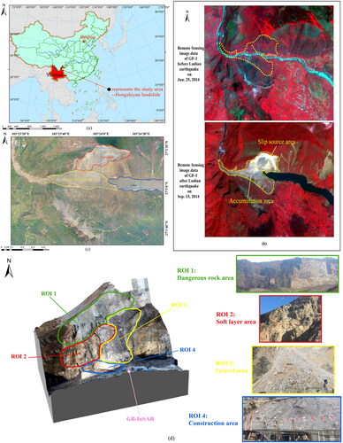
The area monitored by ground-based radar is located northwest of the dammed lake. The monitoring range of radars in this area is set to 50–1000 m. Figure 4(d) shows the DEM stereoscopic map of the whole monitoring area and the magnified images of some key areas, where DEM directly extracts high-precision terrain data based on UAV tilt photography photos. The purple dots in the area represent the location of the radar, using four different colored closure curves to divide the focused study area. Therefore, the entire monitoring area can be divided into the following four sections, and the characteristics of each area are described in further detail：

ROI1 represents the shotcrete area (green boundary). Affected by the earthquake, the rock mass in this area is cracked and relaxed, forming many dangerous rock bodies. This area is approximately 450 m wide and 100 m high, with its highest point approximately 500 m above the surface. It has collapsed in the past, leaving exposed rock walls and posing a risk of secondary collapse, so it is the main area subjected to slope monitoring. According to the engineering treatment research scheme, the slope manager reinforced the wall by spraying concrete onto the surface and erecting a protective net to prevent rocks from falling.

ROI2 represents the soft layer area (red boundary). The weak interlayer in this area is located in the middle of the right bank high slope, which is the main control structural surface of the right bank high slope, and its damage mode is mainly the collapse type of dumping. According to the structural diagram of the field investigation, the existence of the weak interlayer plays a key role in the evolution of the right bank slope. The occurrence is roughly parallel to the layer, inversely inclined to the slope, with a soft structural texture and a small amount of vegetation attached to the surface. As there are several instances of large drilling equipment below the area, the vibration of the equipment will have a certain impact on the rock above the slope, which will pose a major threat to the safety of the equipment and personnel below.

ROI3 represents the gravel area (yellow boundary). In this area, under the action of earthquakes, the rock mass in the middle and lower parts of the slope slides and loses stability along the weak interlayer, after which the rock mass in the middle and upper parts of the slope collapses and is destroyed over a wide area due to the loss of support from the upper part. The average slope of the broken rock area is approximately 50°–60°, which is mainly composed of soft clay and some remaining rock blocks. The lower elevation is subject to sliding failure with rainfall and artificial activities. The rock mass is severely damaged and broken, and rockfall instability phenomena at the top remnant of the back scarp pose a substantial threat to construction workers and mechanical equipment at the base of the slope.

ROI4 represents the ground construction area (blue boundary). To ensure safety during the construction of the landslide dam seepage prevention system at the lower part of the high slope on the right bank, a 7 m high protective wall and a high passive protective net are arranged on the construction platform of the landslide dam cutoff wall on the high slope. Therefore, there is a large amount of drilling equipment working in this area. This equipment and human activities will threaten slope stability. In addition, this area is used to house the equipment and materials needed for the slope management project as well as for the livelihood of the staff.

In summary, the local climate in Yunnan can easily lead to landslide geological hazards due to influencing factors such as rainfall and construction activities. Therefore, it is necessary to carry out comprehensive and continuous monitoring of ROI1, ROI2, and ROI3 on the high right bank slopes to ensure that the dammed lake remediation works at ROI4 are carried out safely and smoothly and that personnel and property are protected from injury and loss.

3.2. Dataset acquisition

3.2.1. Satellite InSAR

The SBAS-InSAR technique is an analysis method for Multimaster-image InSAR time series that utilizes interferometric pairs of small time–space baselines to generate the surface deformation. The SBAS method obtains the surface deformation information along the radar line of sight (LOS), but for mountainous areas, the deformation rate in the LOS direction is not sufficient to truly reflect the deformation of the slope. The deformation rate in the LOS direction is converted to the deformation rate along the slope direction by the following equation (Zhang et al. 2018): (12) $$V_u=\frac{V_{\mathit{los}}+V_{\mathit{slope}}\hspace{0.17em}\sin \hspace{0.17em}\theta \cos \left[\delta -\left({\alpha }_s-\frac{3}{2}\pi \right)\right]}{\cos \theta }$$(12) (13) $$V_{\mathit{slope}}=\frac{V_{\mathit{los}}}{\cos \beta }$$(13) (14) $$\cos \beta =n_{\mathit{los}}\times n_{\mathit{slope}}$$(14) (15) $$n_{\mathit{los}}=(-\sin \theta \cos {\alpha }_s,\sin \theta \sin {\alpha }_s,\cos \theta )$$(15) (16) $$n_{\mathit{slope}}=(-\sin \alpha \cos \phi ,-\cos \alpha \cos \phi ,\sin \phi )$$(16)

In Equations (12)–(16), $V_{\mathit{slope}}$ represents the deformation rate along the slope direction; $V_{\mathit{los}}$ represents the deformation rate in the LOS direction; $V_u$ represents the deformation rate in the vertical direction; $\alpha$ represents the aspect of the slope; $\phi$ represents the gradient of the slope; $\theta$ represents the radar incidence angle; $\delta$ represents the azimuth of the landslide; $\beta$ represents the included angle of the apparent slope; and ${\alpha }_s$ represents the flying direction of the radar satellite, with positive ascending orbit data and descending orbit data. To avoid an extremely abnormal absolute value during the conversion from $V_{\mathit{los}}$ to $V_{\mathit{slope}},$ Herrera proposed a fixed threshold for when $\cos \beta =\pm 0.3$ such that $V_{\mathit{slope}}$ cannot be greater than 3.33 times $V_{\mathit{los}};$ i.e. when $-0.3<\cos \beta <0,$ $\cos \beta =-0.3,$ and when $0<\cos \beta <0.3,$ $\cos \beta =-0.3$ (Herrera et al. 2013).

All SBAS steps were processed using SARscape software (Berardino et al. 2002). For a small number (< 20) of images, the SBAS technique was selected to obtain deformation results. In this paper, a total of 14 Sentinel-1A satellite images acquired from 21 January 2019 to 1 August 2019 were obtained. SBAS-InSAR technology is used for clipping, interference processing, orbit refining, and inversion to obtain the line of sight (LOS) directional deformation rate map in the study area, which is converted into the slope directional deformation rate map through the formula.

3.2.2. UAV

UAV photogrammetry is widely used for geological surveys and disaster monitoring due to its flexibility, low cost, and high spatial and temporal resolution (Galarreta et al. 2015; Guo et al. 2020). This study used a DJI M600-Pro UAV with five Zenmuse X5 tilt photography camera sets to acquire two periods of UAV images on 29 December 2018 and 29 July 2019, i.e. prelandslide and postlandslide images during the long time series of continuous monitoring in this study area. The December and July flights yielded a total of 190 and 200 high-overlap aerial images of different angles, respectively, all with a pixel size of 4608 × 3456 and an average ground resolution of 3 cm (see Table 2 for detailed parameters). After preprocessing and image registration of UAV aerial images, a high-resolution DOM (digital orthophoto map) and DSM (digital surface model) in the study area were obtained. The error after two image registrations met the requirements for subsequent visual interpretation and multisource data fusion.

Table 2. The parameters of the M600-Pro-type UAV and Zenmuse-X5 camera lenses.

UAV flight capability	Actual endurance	Aerial camera	Camera parameters
Maximum flight altitude	2500	Effective pixel	16 megapixels
Maximum allowable wind speed	8 m/s	Equivalent focal length	30 mm
Maximum pitch angle	25°	Camera memory	64 GB
Task load	6 kg	Maximum resolution	4608 × 3456

3.2.3. Gb-InSAR

The deformation measurement principle of ground-based synthetic aperture radar interferometry (GB-InSAR) is similar to that of spaceborne InSAR. This measurement is characterized by the integration of synthetic aperture radar, interferometry technology, stepped frequency continuous wave (SFCW) technology, and other advanced technologies (Bardi et al. 2016; Carlà et al. 2018; Carla et al. 2019). According to the actual situation of the high slope of the Hongshiyan landslide dam, GB-InSAR monitoring equipment is reasonably arranged after the survey to realize large-scale continuous deformation monitoring of the right bank slope. The maximum monitoring distance of the GB-InSAR is 4 km, the displacement and deformation extraction accuracy is better than ± 0.04 mm, and the image resolution is better than 0.2 m in the range direction and 5.5 mrad in the azimuth direction. Table 3 shows some parameters of the monitoring system.

Table 3. Equipment technical index.

Frequency	Bandwidth (MHZ)	Monitoring scope (°)	Operating distance (km)	Repetition time (min)	Range resolution (m)	Azimuth resolution (mrad)
Ku	500	30 ∼ 80	Maximum 5	4 ∼ 10	$\Delta R=\frac{C}{2B}$ = 0.3	${\delta }_{\mathit{angle}}=\frac{\lambda }{2L_s}\gamma$ = 5.4

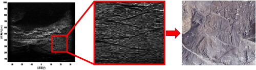
Due to the typical top-hard and bottom-soft structural characteristics of the rock masses developed on the high slopes of the right bank, the radar equipment monitoring station was located on the right bank slope 607 m from the area to be measured. This observation is in continuous observation mode with a fixed orbit, a short observation distance (<600 m), and a zero spatial baseline; therefore, GB-InSAR data processing does not require image alignment and topographic phase compensation. In summary, Figure 5 shows the comparison between the radar echo amplitude map and UAV image map in the monitoring area. Some topographical features of the monitored area can be seen in the radar images, and the amount of vegetation in the radar-monitored area is minimal. Therefore, the radar images from the ground-based DInSAR system used in this study are of good quality.

Figure 5. Monitoring-area radar images (left, middle) and UAV image (right).

3.3. Data processing

3.3.1. Sbas-InSAR processing

In this study, a set of 13 sentinel-1A images from 21 January 2019 to 1 August 2019 were processed in the SARScape module. Using the SBAS-InSAR technique, the annual average surface deformation rate (VLOS) of the study area in the line-of-sight direction was obtained by a series of computational processes, such as master–slave image selection, image alignment, interferogram generation, high-coherence point selection, noise removal, baseline estimation, deleveling effect, phase decoupling, deformation estimation, atmospheric delay removal, and ground mile coding. Combined with the analysis of remote sensing images, the landslide areas of interest ROI1 to ROI4 have a low density of surface vegetation cover, a high number of coherent points, a good interference effect and a more obvious rate accumulation. Negative values of the deformation rate in the graph indicate that the deformation point is moving away from the satellite sensor, while positive values indicate that the deformation point is moving closer to the satellite sensor. The InSAR LOS deformation analysis results show that the deformation values in Figure 6 are negative, indicating that the overall landslide slides downward toward the Niulan River, which is in line with the movement forces governing the landslide mass. Deformation in the study area is largest in the red region, where the deformation rate is ≥ 104.85 mm/yr.

Figure 6. (a) and (b) Deformation rate map (LOS direction) from January 2019 to August 2019; (c) deformation rate map (slope direction) from January 2019 to August 2019; (d) deformation rate map (vertical direction) from January 2019 to August 2019.

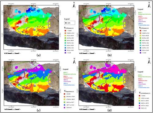
To verify the reliability of the monitoring results, the GPS monitoring data deployed in the study area from September 2018 to July 2019 were selected to validate the SBAS-InSAR monitoring results with ten GPS monitoring points, P1 to P10 (as shown in Figure 6(a)). As the GPS monitoring points do not correspond to the SBAS-InSAR monitoring results, a buffer zone with a radius of 50 m was delineated at the center of the GPS monitoring points, and the mean SBAS-InSAR deformation rate within the buffer zone was counted. Using the 10 GPS monitoring points on the landslide surface, the mean values of the movement rates of the buffers for P1 to P10 were decomposed in the plumb line direction to obtain the vertical variation rate V_vertical along the landslide surface (as shown in Figure 6(d)). Based on the measured data of the movement of the GPS observation points on the landslide surface, the horizontal combined displacement and vertical displacement of each GPS observation point was obtained, and the vertical change rate V_Z of the monitoring points was calculated. Without considering the difference between the angle of incidence of the radar line of sight and the slope of the landslide, only the vertical rate of change along the landslide surface is analyzed in this paper. Table 4 shows that the movement rate of GPS monitoring points in the vertical direction and the vertical change rate of the SBAS-InSAR landslide surface are in good agreement, and the error is within 20 mm/yr. SBAS-InSAR technology can thus be used for macroscopic change monitoring of landslide movement trends in the study area. The mean annual rate (V_slope) and the mean annual vertical rate (V_vertical) of landslides along the right bank of Hongshiyan are shown in Figures 6(c) and (d). The decoded areas of strong deformation are in general agreement with the LOS direction, but there are large differences in the deformation rate values, with the overall deformation rate in the slope direction being much higher than that in the LOS direction, with a maximum deformation rate of 201.58 mm/yr in the slope direction.

Table 4. SBAS-InSAR versus GPS monitoring data validation (mm/yr).

Point number	Vvertical	Vz	Difference
P1	−19.2784	−12.7841	6.4943
P2	−25.7519	−14.0427	11.7092
P3	−19.6571	−13.1125	6.5446
P4	−65.8456	−46.2145	19.6311
P5	−125.7324	−105.9572	19.7752
P6	−116.7417	−105.4218	11.3199
P7	−103.5482	−91.8849	11.6633
P8	−99.4185	−84.1204	15.2981
P9	−105.7418	−94.5486	11.1932
P10	−127.7716	−114.9813	12.7903

ROI1 is the area of shotcrete, which makes the treated zone of dangerous rock more stable due to the surface sprayed concrete and the protective mesh reinforcing the wall. As seen in Figure 6, the accumulated displacement change at point E in this area is relatively stable, and the deformation rate is in a long-term stable state. ROI2 is a soft layer area that consists mainly of soft clay and some remaining rock masses. The cumulative displacement of point B reached 200 mm/yr in the slope direction. This indicates that the red part of this area has undergone large deformation, so this area was as a focus for later research. ROI3 is a gravel area due to the presence of many different sizes of rubble on the slope, the largest of which is over 90 m in diameter. Based on the deformation rate of the area near point A, this region is among the more unstable parts. As point C is on the part of the right bank slope that is already close to the landslide dam, most of the deformation is due to the long-term accumulation of debris on the slope. The trend in deformation rate is similar at points A and C, indicating that the debris in the vicinity of A is sliding heavily along the slope. This process takes the form of softening and erosion of the rock structure by rainfall, which destabilizes the rock and causes slope debris to slide. ROI4 is the ground construction area where multiple drilling rigs are located to carry out manual operations during the monitoring period. The gravity retaining walls and passive fences intercepted many small debris accumulations. In this case, the increase in the deformation rate is mainly due to the strong pushing action at the foot of the slope.

3.3.2. Gb-InSAR processing

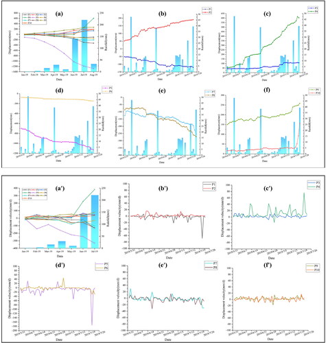
The atmospheric impact is negligible due to the close monitoring distance of the ground-based radar placement and the lack of water separation. The preidentified regions of interest ROI1 to ROI4 were analyzed in further detail based on a priori knowledge. The GB-InSAR images were synthesized based on differential interference techniques, and Figure 7(a) depicts the cumulative deformation maps generated by GB-InSAR throughout the acquisition period. Obviously, from the black circled part of the figure, you can see that it is the area with large deformation changes. The monitoring period was from 1 January 2019 to 23 July 2019, during which time five large deformations were observed from ROI1 to ROI4, with positive deformations indicating movement toward the radar site and negative deformations indicating movement away from the radar site. To specifically analyze the slope deformation, some representative and evenly distributed typical feature monitoring points were selected in these 5 large deformation areas. Figure 7(a) shows 10 typical feature monitoring points (P1∼P10), where each area contains 2 points, while the enlarged views of selected monitoring features are shown in Figure 8(b)–(e):

Figure 7. Cumulative displacement map of GB-InSAR campaigns.

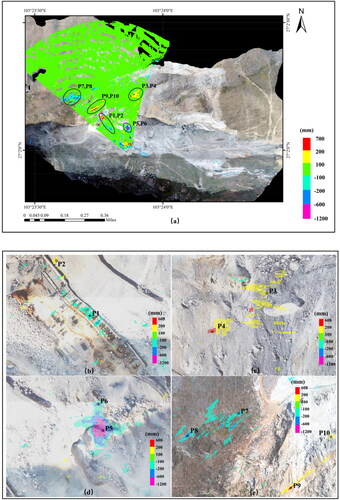
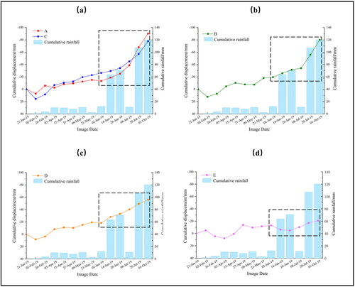
Figure 8. Response of SBAS-InSAR time-series deformation results to rainfall for typical feature points A, B, C, D, and E.

• P1 and P2: located in the ground construction area (ROI4)

• P3 and P4: located in the top area of the gravel zone (ROI3)

• P5 and P6: located in the bottom area of the gravel zone (ROI3)

• P7 and P8: located to the west of the softly interbedded area and contain little vegetation (ROI2)

• P9 and P10: located to the east of the weakly interbedded area (ROI2).

Two areas of significant activity existed on the landslide: P9 and P10 in the central left-hand ROI2 area and P3 and P4 in the upper central right-hand ROI3 area. These two deformation processes are mainly caused by the sliding of rainfall-induced piles of loose soil under the action of gravity. The deformation of the middle and upper parts of the slope is large, and there is an overall sliding trend; therefore, this area is used as the starting target point for displacement tracking and trajectory prediction. The overall deformation of the reinforcement in the upper ROI1 area of the slope after concrete injection is relatively stable, but there is a large deformation near points P5 and P6 in the lower and middle ROI3 areas on the right. According to the magnified view (Figure 9(d)), the collapse area depression is caused by falling gravel in this area, and the positive deformation at the lower part of point P5 is caused by the accumulation of scattered landslide mass. The lower part of the slope is relatively stable, but on the upper left side of the lower part of the ROI4 area, the topsoil is floating soil from previous landslides, which slides rapidly under the action of the slope flow, resulting in a weak echo strength and some large deformation units.

Figure 9. Cumulative deformation curves (a–f) and displacement velocity versus curves (a’–f-) over time at typical monitoring features.

4. Results and discussion

In this study, we present a new methodology for analyzing slope stability based on three techniques: InSAR, UAV, and GB-InSAR. The SBAS-InSAR technique is combined with the overall analysis of the study area to identify the ROIs with large deformation and the starting target points, and the fusion results of RDD and DSM data are used to fit the deformation surface field of the region. The gradient descent approach is executed to obtain the running trajectory points of the target masses so that the main slip direction and displacement trajectory of the fine parts in the study area can be predicted. The experimental results show that the method can exactly identify the deformation area, especially in the case of a fast-changing deformation trend. These findings can provide more accurate monitoring area results to aid in the rapid control and prevention of landslide hazards by analyzing the minimum pixel grid (i.e. points) in the monitored area as the smallest spatial unit at a time interval of minutes.

Based on the results of SBAS-InSAR, points A, B, C, D, and E with large deformation characteristics were selected within the four regions of interest (ROI1-ROI4) of the landslide line-of-sight deformation rate map (Figure 6(b)). The historical cumulative displacement curves for the corresponding points were then drawn and compared with the cumulative rainfall data from the rainfall stations in the study area for each month from January 2019 to August 2019 (as shown in Figure 8). As seen in Figure 8(d), the deformation rate is in a long-term stable state, and the deformation amplitude is controlled within the range of [−0.5, +0.5] mm. As seen in the black box, the heavy rainfall in June and July did not affect the stability of the area, indicating that the entire ROI1 area did not experience significant deformation during the monitoring period. As shown in Figure 8(b), the impact of rainfall on the region is relatively large. At point B, there is a slow increase in its cumulative displacement during the nonflood period from January 2019 to June 2019, but the sharp increase in rainfall starting in June 2019 causes a significant leap-step acceleration in point B deformation. The cumulative displacement of point B reached 62 mm in June and July, corresponding to a cumulative rainfall of 363 mm in these two months. This finding indicates that the red part of this area underwent large deformation and that the deformation trend has a good response pattern with rainfall. Figure 8(a) shows a cumulative displacement of −91 mm over the entire 7-month monitoring period and a deformation rate of 36 mm/month during the heavy rainfall periods in June and July. The black box shows an exponential increase in the cumulative displacement in June and July, indicating that the debris in the vicinity of A is sliding heavily along the slope due to rainfall and human activities. The cumulative displacement of the monitoring features located at ROI4 over the total period was calculated as follows: P1 was −217.63 mm, and P2 was 189.25 mm. The cumulative displacement in June and July was more variable, and the cumulative displacement in these two months was −155.42 mm for P1 and 102.68 mm for P2 (as shown in Figure 8(c)).

Time series analysis of slope deformation was carried out by selecting two feature points in each area with large deformation from the GB-InSAR monitoring results (Figure 9). As shown in Figure 9(a), the timing of the large changes in deformation roughly starts from the flood season in June in the study area. The main factor inducing slope deformation is the water entering the slope and triggering the later landslide, which is in line with the local rainfall monitoring and the trend results of SBAS-InSAR monitoring. Figure 9(b)–(f) represent the time series plot of cumulative displacement on days 1 June 2019 to 23 July 2019 for each typical feature point, and Figures 9(a’)–(f’) show the displacement velocity curve corresponding to each typical feature point over time. The instantaneous displacement velocities of the target points in the ROI4 area are shown in Figure 9(b’) and are relatively stable, with values of approximately ±20 mm/d. P1 produced a deformation rate of −68.79 mm/d on 20 July 2019 due to the movement of machinery and equipment within the ground work area caused by a small rock slide on that date. The cumulative displacement of the monitoring features located at ROI3 is shown in Figure 9(c), which shows an overall downward movement along the slope, with an accelerating trend during rainfall. The surface rock within the area was unstable during the monitoring period, and the cumulative displacement at each point over the total period was calculated as 193.98 mm for P3 and 652.77 mm for P4. As the rainfall increases in this area, the cumulative shape of the variables is smoother at point P3. The cumulative displacement at point P4 reached 602.14 mm in June and July, and the daily deformation rate at this point showed significant and highly erratic jumps and peaked at 76.21 mm/d on 20 July. The cumulative displacement of the monitored feature points located at ROI3 is shown in Figure 9(d), and the overall deformation variables are dominated by subsidence slips. The cumulative displacements at point P5, where the surface rock is loosely deformed, are calculated as −1192.56 mm for P5 and −216.39 mm for P6. As seen from the graph, the cumulative displacement at point P5 in June and July was −575.64 mm. From 11 July onward, the deformation rate gradually increased, reaching a maximum of −175 mm/d on the morning of 20 July when the landslide occurred, after which the deformation rate returned to the normal range. The cumulative displacement of the monitored feature points located at ROI2 is shown in Figure 9(e) and (f). The deformation variables at points P7, P8, P9, and P10 are small and basically in a steady state, and their daily deformation rates also remain stable.

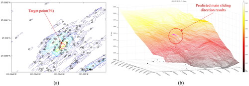
Based on the above results, point A (corresponding to P4 of the GB-InSAR results), where the SBAS-InSAR deformation variables are large, was selected for validating the method of mass displacement tracking and displacement trajectory prediction. The morphological mutation at P4 on 10 June 2019 was used as the starting time point, and the endpoint was 22 July 2019. The fitted deformation surface field proposed in Section 2 of this paper was constructed using the day cumulative displacement data, and the trajectories obtained by solving the deformation field by the gradient descent method were connected (a schematic diagram of the actual deformation of the region with the fitted deformation field is shown in Figure 10). Figure 11(a) shows an orthographic image of the contours of the deformation field in the landslide area. The density of the contours tracks the gradient: the denser the contours are, the greater the rate of change of the data and the greater the gradient. Conversely, the smaller the rate of change of the data, the smaller the gradient. The direction and distance of the fastest change in deformation (i.e. the distance to the contour with the smallest value) is searched for in the downward, leftward, and rightward directions according to the change in contour. The overall sliding azimuth is the angle between the synthetic vector of two of the motion vectors (lower left or lower right) and due north, which is the main sliding direction of the landslide. Each of these sliding azimuths is clockwise for positive clamping angles and counterclockwise for negative clamping angles. The above algorithm gives the main slide direction of the 20 July landslide as −47.6026° from due north (as shown in Figure 11(b)).

Figure 10. Results of deformation surface field fitting. (a) 3 D scatter plot of the deformation region; (b) schematic of the real deformation region; (c) 3 D smoother fit of the regional deformation field; (d) regional deformation surface field fitted with the Lorentz2D function.

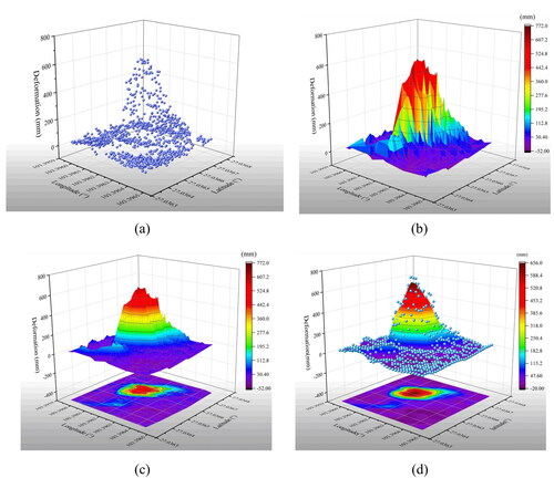
Figure 11. (a) Fitted deformation surface field contours and target starting point maps; (b) predicted main slip direction and displacement trajectory maps.

The method can also set the time interval, for example, by an hourly interval for a more refined prediction of the main slide direction of the landslide, using the landslide data from 0:00 to 12:00 on 20 July 2019 (as shown in Figure 12). Dividing this period into 12 one-hour intervals, this study finds the maximum regional displacement trajectory for each period, with a contour interval of 1 mm. The contoured terrain deformation data are combined with the in situ UAV image data as a basis for the final presentation of the tracking effect of the mass point in 3 D space. The slope in Figure 12 shows the topographic data of the landslide area, and the vertical axis indicates the elevation. The contours are plotted on the XOY plane, while the deformation trajectory is plotted on the 3 D slope. At this point, the researcher can see the topographic information, the regional deformation information, and the direction of movement of the masses at each time in the diagram at the same time.

Figure 12. Hourly step-by-step chart of demonstration data from 0:00 to 12:00 on 20 July 2019.

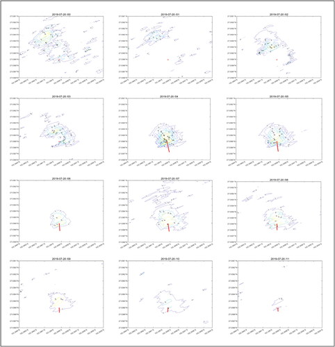
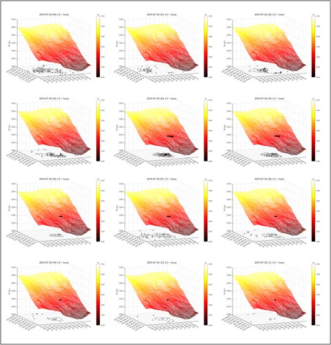
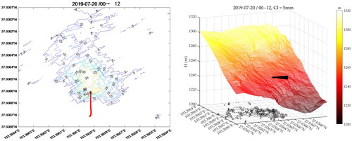
As seen from the figure, the degree of regional deformation varies from time to time. We obtained the maximum regional displacement trajectory for each period by employing the method described in Section 2, which is the red trajectory in Figure 13. On the one hand, we consider that the trajectory of the masses in the landslide will obey the regional maximum displacement trajectory, especially at locations where the deformation is large. Therefore, the direction of movement of the mass at a given time should be the same as the direction of the maximum displacement trajectory of the region. However, the amount of displacement of the masses varies from time to time due to the different degrees of deformation. Since the actual displacement of the masses in a short period may not be sufficient to be shown on a radar pixel-level plot, we have zoomed in here on the actual amount of movement. The length of the red trajectory in the diagram is proportional to the displacement of the mass so that during periods of greater deformation, the trajectory is longer. Conversely, almost no trajectory appears, so the magnitude of the movement of the mass can be visualized. As seen from the 12 hourly diagrams, the direction of movement of the mass is relatively stable, and the amount of movement fluctuates considerably with the trend of deformation. By summing the trajectories for the 12 time periods, we obtain the total trajectory in Figure 13, where the contour interval is 5 mm. The total trajectory did not show a large change as the mass moved in a relatively consistent direction from one moment to the next.

Figure 13. General drawing of displacement tracking and trajectory prediction of 0–12 points on July 20, 2019.

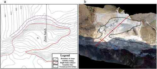
In summary, this study uses the fusion of deformation data with topographic data, local least squares surface fitting, and gradient descent to identify and predict the main slip direction. This approach was verified using actual data from the monitoring of the Hongshiyan slopes in Yunnan, where a small landslide event occurred on 20 July 2019, and the predicted results matched the site conditions. As shown in Figure 14(a), according to the results proposed by Zongliang Zhang and other researchers, the boundary line of the right bank collapse can be seen in the zoning stability diagram of the Hongshiyan rock collapse mass (Zhang et al. 2020). After visual interpretation of the DSM map obtained by the UAV, the depression at the back edge and the convex point at the front edge of the landslide can be seen. The conventional monitoring method shows that the red line in Figure 14(b) is the main axis of the landslide, and it is also the main sliding direction of the landslide based on the empirical method. The included angle of the main sliding direction measured by ArcGIS is −41.0129°. The specified sliding azimuth angle is positive clockwise and negative counterclockwise. Therefore, the main sliding direction of the landslide obtained based on this study is consistent with the results of the empirical method, with an error of approximately 6 degrees. The reason for this error is that there is a time difference between the DSM data obtained by the UAV and this small landslide event, but the results verify the rationality of the proposed method for solving the main sliding direction of the landslide in this study. The advantages of the high temporal resolution of ground-based radar monitoring are evident due to the short duration of the deformation surge period before damage occurs on brittle rock slopes, which is often only a few hours, especially when the mass of the damaged rock is small. For such slopes, the frequency of monitoring data collection needs to be increased if the damage is to be effectively predicted or inferred, especially in the proximity of damage. The method in this study solves the problem of the previous lack of soundness in the theory of relying on slope body personnel surveys or empirical and semiempirical methods. Especially for complex, dangerous slope bodies, the accuracy of analyzing the main sliding direction only by these empirical and semiempirical methods cannot be guaranteed. The method further enables the use of minute time intervals to construct deformation fields to fit curved fields, avoiding the contact point predictions of traditional methods and demonstrating the method’s value for engineering applications. The prediction of landslide displacement trajectory based on gradient descent method results provides the main slip direction and postslide trajectory prediction of the slope and is applied to the slope antislide design, which is valuable for assessing disaster risks and improving landslide prevention and control effects.

Figure 14. (a) Diagram of the slope stability zone of the right bank collapse; (b) schematic diagram of the main sliding direction of the landslide obtained by the empirical method.

5. Conclusions

Landslide monitoring technology has great social and scientific impact. Currently, many slopes are routinely monitored by ground-based monitoring radar. This study applies GB-InSAR to landslide monitoring, where data acquired by ground-based radar devices are combined with a variety of data, such as geological and geomorphological field surveys, spaceborne SAR, and UAV orthophotography. In this paper, the point in the slope surface deformation monitoring study is taken as the smallest spatial unit to be monitored, and its change process and change characteristics can reflect the microscopic process of disaster change from a microscopic perspective, which is fundamental for disaster change analysis. A method is proposed for predicting the main slide direction and tracking the trajectory of mass displacement movement based on multiple fused data. The main conclusions are as follows:

• In this paper, the spatial and temporal distributions of large deformations on high slopes in the Hongshiyan study area in Yunnan were studied by using 14 Sentinel-1A SAR images with the SBAS-InSAR technique. By characterizing the areas where larger deformation points are clustered in the overall deformation data of the study area with this technique, four general areas and regions of interest (ROI1-ROI4) where larger landslides occur were initially identified.

• The starting target point A of the landslide (corresponding to P4 of the GB-InSAR results) was finally selected through data analysis of the larger deformation points in the multiperiod ground-based radar deformation data, based on the single-point deformation rate curve data and the experience of the topography of the region.

• With the surface fitting of the deformation field near the target point (P4) as well as the use of the mass displacement tracking prediction method proposed in this paper, the main slip direction and displacement trajectory of the subareas of the study area can be accurately predicted, and the reliability of the method is verified according to the actual situation of the landslide site.

The test shows that the GB-InSAR system has the advantages of high precision, long distance, large measurement range, etc., and has unique advantages for the monitoring of large landslides and other geological disasters. While reducing the influence of the error from the data sources is the most efficient way to improve the monitoring accuracy, improving the measurement accuracy under the influence of surface vegetation still requires further research and development. Therefore, determining how to reduce and minimize the influence of various factors from the raw data is our next research focus.

Authors’ contributions

All authors contributed to the manuscript and discussed the results. Jiabao Wang and Tianjie Lei developed the idea that led to this paper. Jiabao Wang performed Sentinel-1A data processing, designed the experiments, analyzed the data, and wrote the first draft. Wenkai Liu provided critical comments and contributed to the final revision of the paper. Yijin Chen, Baoyin Liu, and Jianwei Yue gave suggestions for modifications to the manuscript. In addition, all authors contributed to the final revision of the manuscript.

Acknowledgments

We would like to thank Tong Jiang of the College of Surveying and Geo-informatics, North China University of Water Resources and Electric Power (Zhengzhou), for providing comments and writing suggestions. We would also like to thank the anonymous reviewers and the editors for their comments.

Disclosure statement

No potential conflict of interest was reported by the author(s).

Data availability statement

Self‐collected datasets that support the findings of this study are available from the corresponding author upon reasonable request.

Additional information

Funding

This work was supported by The Agricultural Science and Technology Innovation Program of Chinese Academy of Agricultural Sciences.

References

- Alamdar F, Kalantari M, Rajabifard A. 2015. An evaluation of integrating multisourced sensors for disaster management. Int J Digital Earth. 8(9):727–749.
- Bardi F, Raspini F, Ciampalini A, Kristensen L, Rouyet L, Lauknes TR, Frauenfelder R, Casagli N. 2016. Space-borne and ground-based InSAR data integration: the angstrom knes test site. Remote Sens. 8(3):237.
- Benoit L, Briole P, Martin O, Thom C, Malet JP, Ulrich P. 2015. Monitoring landslide displacements with the Geocube wireless network of low-cost GPS. Eng Geol. 195:111–121.
- Berardino P, Fornaro G, Lanari R, Sansosti E. 2002. A new algorithm for surface deformation monitoring based on small baseline differential SAR interferograms. IEEE Trans Geosci Remote Sens. 40(11):2375–2383.
- Carlà T, Farina P, Intrieri E, Ketizmen H, Casagli N. 2018. Integration of ground-based radar and satellite InSAR data for the analysis of an unexpected slope failure in an open-pit mine. Eng Geol. 235:39–52.
- Carla T, Intrieri E, Raspini F, Bardi F, Farina P, Ferretti A, Colombo D, Novali F, Casagli N. 2019. Perspectives on the prediction of catastrophic slope failures from satellite InSAR. Sci Rep. 9(1):18733.
- Carla T, Tofani V, Lombardi L, Raspini F, Bianchini S, Bertolo D, Thuegaz P, Casagli N. 2019. Combination of GNSS, satellite InSAR, and GBInSAR remote sensing monitoring to improve the understanding of a large landslide in high alpine environment. Geomorphology. 335:62–75.
- Casagli N, Catani F, Del Ventisette C, Luzi G. 2010. Monitoring, prediction, and early warning using ground-based radar interferometry. Landslides. 7(3):291–301.
- Chen D, Li H, Zhu K. 2021. Vector sum analysis method for slope stability based on new main sliding trend direction. Rock Soil Mech. 42:9.
- Chen G, Zhang Y, Zeng R, Yang Z, Chen X, Zhao F, Meng X. 2018. Detection of land subsidence associated with land creation and rapid urbanization in the Chinese Loess Plateau using time series InSAR: a case study of Lanzhou New District. Remote Sens. 10(2):270.
- Chung C-C, Lin C-P. 2019. A comprehensive framework of TDR landslide monitoring and early warning substantiated by field examples. Eng Geol. 262:105330.
- Cigna F, Tapete D. 2021. Sentinel-1 big data processing with P-SBAS InSAR in the geohazards exploitation platform: an experiment on coastal land subsidence and landslides in Italy. Remote Sens. 13(5):885.
- Dai K, Li Z, Xu Q, Burgmann R, Milledge DG, Tomas R, Fan X, Zhao C, Liu X, Peng J, et al. 2020. Entering the era of earth observation-based landslide warning systems: a novel and exciting framework. IEEE Geosci Remote Sens Mag. 8(1):136–153.
- Dai Z, Wang F, Cheng Q, Wang Y, Yang H, Lin Q, Yan K, Liu F, Li K. 2019. A giant historical landslide on the eastern margin of the Tibetan Plateau. Bull Eng Geol Environ. 78(3):2055–2068.
- Di Matteo L, Romeo S, Kieffer DS. 2017. Rock fall analysis in an Alpine area by using a reliable integrated monitoring system: results from the Ingelsberg slope (Salzburg Land, Austria). Bull Eng Geol Environ. 76(2):413–420.
- Dikshit A, Satyam N. 2019. Probabilistic rainfall thresholds in Chibo, India: estimation and validation using monitoring system. J Mt Sci. 16(4):870–883.
- Dong J-J, Lee W-R, Lin M-L, Huang A-B, Lee Y-L. 2009. Effects of seismic anisotropy and geological characteristics on the kinematics of the neighboring Jiufengershan and Hungtsaiping landslides during Chi-Chi earthquake. Tectonophysics. 466(3–4):438–457.
- Dong J, Zhang L, Tang M, Liao M, Xu Q, Gong J, Ao M. 2018. Mapping landslide surface displacements with time series SAR interferometry by combining persistent and distributed scatterers: a case study of Jiaju landslide in Danba, China. Remote Sens Environ. 205:180–198.
- Dong W, Zhu H, Sun Y, Shi B. 2016. Current status and new progress on slope deformation monitoring technologies. J Eng Geol. 24(6):1088–1095.
- Ehteshami-Moinabadi M, Nasiri S. 2019. Geometrical and structural setting of landslide dams of the Central Alborz: a link between earthquakes and landslide damming. Bull Eng Geol Environ. 78(1):69–88.
- Euillades LD, Euillades PA, Riveros NC, Masiokas MH, Ruiz L, Pitte P, Elefante S, Casu F, Balbarani S. 2016. Detection of glaciers displacement time-series using SAR. Remote Sens Environ. 184:188–198.
- Galarreta JF, Kerle N, Gerke M. 2015. UAV-based urban structural damage assessment using object-based image analysis and semantic reasoning. Nat Hazards Earth Syst Sci. 15(6):1087–1101.
- Guo C, Qiang XU, Peng S, Sun T. 2020. Application research of UAV photogrammetry technology in the emergency rescue of Baige landslide. J Catastrophol. 35:8. SUN: ZHXU.0.2020-01-041.
- He H, Li S, Liu M, Huang H. 2016. Research on landslide spatial distribution in Ludian earthquake disaster area. J Catastrophol. 31(01):92–95.
- Herrera G, Gutiérrez F, García-Davalillo JC, Guerrero J, Notti D, Galve JP, FernáNDez-Merodo J, Cooksley G. 2013. Multi-sensor advanced DInSAR monitoring of very slow landslides: the Tena Valley case study (Central Spanish Pyrenees). Remote Sens Environ. 128:31–43.
- Hong H, Ilia I, Tsangaratos P, Chen W, Xu C. 2017. A hybrid fuzzy weight of evidence method in landslide susceptibility analysis on the Wuyuan area, China. Geomorphology. 290:1–16.
- Intrieri E, Raspini F, Fumagalli A, Lu P, Del Conte S, Farina P, Allievi J, Ferretti A, Casagli N. 2018. The Maoxian landslide as seen from space: detecting precursors of failure with Sentinel-1 data. Landslides. 15(1):123–133.
- Jia G, Buchroithner MF, Chang W, Liu Z. 2016. Fourier-based 2-D imaging algorithm for circular synthetic aperture radar: analysis and application. IEEE J. Sel. Top. Appl. Earth Observ Remote Sens. 9(1):475–489.
- Kawamura K, Ogawa Y, Oyagi N, Kitahara T, Anma R. 2007. Structural and fabric analyses of basal slip zone of the Jin’nosuke-dani landslide, northern central Japan: its application to the slip mechanism of decollement. Landslides. 4(4):371–380.
- Kumar V, Gupta V, Jamir I, Chattoraj SL. 2019. Evaluation of potential landslide damming: case study of Urni landslide, Kinnaur, Satluj valley, India. Geosci Front. 10(2):753–767.
- Lacroix P, Handwerger AL, Bievre G. 2020. Life and death of slow-moving landslides. Nat Rev Earth Environ. 1(8):404–419.
- Lazecky M, Comut FC, Hlavacova I, Gurboga S. 2015. Practical Application of Satellite-Based SAR Interferometry for the Detection of Landslide Activity. In Proceedings of the 1st World Multidisciplinary Earth Sciences Symposium (WMESS), Prague, CZECH REPUBLIC, 2015 Sep 07–11; p. 613–618.
- Le TS, Chang C-P, Nguyen XT, Yhokha A. 2016. TerraSAR-X data for high-precision land subsidence monitoring: a case study in the historical centre of Hanoi, Vietnam. Remote Sens. 8(4):338.
- Liao B, Wang H. 2014. Design of landslide monitoring system based on Beidou communication. Automat Instrumentat. 29(05):22–25.
- Li Z, Cao Y, Wei J, Duan M, Wu L, Hou J, Zhu J. 2019. Time-series InSAR ground deformation monitoring: atmospheric delay modeling and estimating. Earth-Sci Rev. 192:258–284.
- Li Q, ChaoZeng; Liu W, Wen Z, Li C. 2019. Dynamic discrimination of main slip direction of a highway landslide based on dense multi-point deformation monitoring. Geol Sci and Technol Inform. 38(04):231–239.
- Li Y, Jiao Q, Hu X, Li Z, Li B, Zhang J, Jiang W, Luo Y, Li Q, Ba R. 2020. Detecting the slope movement after the 2018 Baige Landslides based on ground-based and space-borne radar observations. Int J Appl Earth Observ Geoinform. 84:101949.
- Lin CH, Liu D, Liu G. 2019. Landslide detection in La Paz City (Bolivia) based on time series analysis of InSAR data. Int J Remote Sens. 40(17):6775–6795.
- Liu C, Chen C. 2020. Achievements and countermeasures in risk reduction of geological disaster in China. J Eng Geol. 38(04):231–239.
- Liu SJ, Guo MW, Chun-Guang LI. 2018. Determination of main sliding direction for three-dimensional slope. Rock Soil Mech. 39(S2):37–44.
- Lu P, Han J, Li Z, Xu R, Li R, Hao T, Qiao G. 2020. Lake outburst accelerated permafrost degradation on Qinghai-Tibet Plateau. Remote Sens Environ. 249:112011.
- Lv Q, Liu Y, Yang Q. 2017. Stability analysis of earthquake-induced rock slope based on back analysis of shear strength parameters of rock mass. Eng. Geol. 228:39–49.
- Mazzanti P. 2011. Displacement monitoring by terrestrial SAR interferometry for geotechnical purposes. Geotech News. 29:25–28.
- Nie D, Wang H, Wang X, Meng L. 2019. Crack trajectory analysis of trailing edge of landslide based on image processing. Comput Eng Appl. 55:5.
- Qiu J, Wang X, He S, Liu H, Lai J, Wang L. 2017. The catastrophic landside in Maoxian County, Sichuan, SW China, on June 24, 2017. Nat Hazards. 89(3):1485–1493.
- Raspini F, Bardi F, Bianchini S, Ciampalini A, Del Ventisette C, Farina P, Ferrigno F, Solari L, Casagli N. 2017. The contribution of satellite SAR-derived displacement measurements in landslide risk management practices. Nat Hazards. 86(1):327–351.
- Segoni S, Piciullo L, Gariano SL. 2018. A review of the recent literature on rainfall thresholds for landslide occurrence. Landslides. 15(8):1483–1501.
- Shih PT-Y, Wang H, Li K-W, Liao J-J, Pan Y-W. 2019. Landslide monitoring with interferometric SAR in Liugui, a vegetated area. Terr Atmos Ocean Sci. 30(4):521–530.
- Solari L, Del Soldato M, Raspini F, Barra A, Bianchini S, Confuorto P, Casagli N, Crosetto M. 2020. Review of satellite interferometry for landslide detection in Italy. Remote Sens. 12(8):1351.
- Tian S, Chen N, Wu H, Yang C, Zhong Z, Rahman M. 2020. New insights into the occurrence of the Baige landslide along the Jinsha River in Tibet. Landslides. 17(5):1207–1216.
- Uchimura T, Towhata I, Anh TTL, Fukuda J, Bautista CJB, Wang L, Seko I, Uchida T, Matsuoka A, Ito Y, et al. 2010. Simple monitoring method for precaution of landslides watching tilting and water contents on slopes surface. Landslides. 7(3):351–357.
- Uchimura T, Towhata I, Wang L, Nishie S, Yamaguchi H, Seko I, Qiao J. 2015. Precaution and early warning of surface failure of slopes using tilt sensors. Soils Foundations. 55(5):1086–1099.
- Wang Y. 2016. Characteristics and causes of super-huge secondary geological hazards induced by M6.5 Ludian earthquake in Yunnan. J Catastrophol. 31:4.
- Wang FW, Wang GH, Sassa K, Takeuchi A, Araiba K, Zhang YM, Peng XM. 2005. Displacement monitoring and physical exploration on the Shuping landslide reactivated by impoundment of the Three Gorges Reservoir, China. In Proceedings of the 1st General Assembly of the International-Consortium-on-Landslides, Natl Acad Sci, Keck Ctr, Washington, DC, Oct 12–14, 2005; p. 313–319.
- Xue F, Lv X, Dou F, Yun Y. 2020. A review of time-series interferometric SAR techniques: a tutorial for surface deformation analysis. IEEE Geosci Remote Sens Mag. 8(1):22–42.
- Xu Q, Li W-l, Ju Y-z, Dong X-j, Peng D-l 2020. Multitemporal UAV-based photogrammetry for landslide detection and monitoring in a large area: a case study in the Heifangtai terrace in the Loess Plateau of China. J Mt Sci. 17(8):1826–1839.
- Xu C, Xu X, Shen L, Dou S. 2014. Inventory of landslides triggered by the 2014 Ms6.5 Ludian earthquake and its implications on several earthquake parameters. Seismol Geol. 36:1186–1203. SUN: DZDZ.0.2014-04-020.
- Xu F-g, Yang X-g, Zhou J-w 2017. Dam-break flood risk assessment and mitigation measures for the Hongshiyan landslide-dammed lake triggered by the 2014 Ludian earthquake. Geomat Natural Hazards Risk. 8(2):803–821.
- Yin Y, Zheng W, Liu Y, Zhang J, Li X. 2010. Integration of GPS with InSAR to monitoring of the Jiaju landslide in Sichuan, China. Landslides. 7(3):359–365.
- Yu B, Ma E, Cai J, Xu Q, Li W, Zheng G. 2021. A prediction model for rock planar slides with large displacement triggered by heavy rainfall in the Red bed area, Southwest, China. Landslides. 18(2):773–783.
- Zhang Z, Cheng K, Yang Z, Peng F. 2020. Key technology of emergency remedy and treatment for Hongshiyan barriers lake dam. Hydropower and Pumped Storage. 6:11. SUN: DBGC.0.2020-02-002.
- Zhang XD, Chen JP, Huang RQ, Yan M, Ding HJ. 2005. Study of deformation features of Gapa landslide using FLAC-3D. Rock Soil Mech. 9(01):131–134.
- Zhang Y, Meng X, Jordan C, Novellino A, Dijkstra T, Chen G. 2018. Investigating slow-moving landslides in the Zhouqu region of China using InSAR time series. Landslides. 15(7):1299–1315.
- Zhang Y-g, Tang J, Liao R-p, Zhang M-f, Zhang Y, Wang X-m, Su Z-y 2021. Application of an enhanced BP neural network model with water cycle algorithm on landslide prediction. Stoch Environ Res Risk Assess. 35(6):1273–1291.
- Zhou X, Chen Z, Yu S, Wang L, Deng G, Sha P, Li S. 2015. Risk analysis and emergency actions for Hongshiyan barrier lake. Nat Hazards. 79(3):1933–1959.
- Zhou L, Guo J, Hu J, Li J, Xu Y, Pan Y, Shi M. 2017. Wuhan surface subsidence analysis in 2015-2016 based on sentinel-1A data by SBAS-InSAR. Remote Sens. 9(10):982.