Flood susceptibility modeling of the Karnali river basin of Nepal using different machine learning approaches

Abstract

The Karnali River Basin (KRB) comprises the longest river in Nepal, located south of the Himalayas. Despite its high susceptibility to floods, the basin lacks detailed studies. Proper floodplain management is essential to reduce the impacts due to rising flood frequency, magnitude, and severity aggravated by climate change. This research applies three machine learning techniques, Support Vector Machine (SVM), Random Forest (RF), and Artificial Neural Networks (ANN), to flood event data from the KRB. Ten flood conditioning factors; Aspect, curvature, distance to a river (DTR), normalized difference vegetation index (NDVI), elevation, slope, rainfall, soil, stream power index (SPI), and topographical wetness index (TWI) were selected based on the multicollinearity test. The parameter performance was evaluated using the Cohen Kappa Score, with NDVI having the greatest influence, followed by elevation, DTR, curvature, and TWI. Based on the Area Under the Curve of Receiver Operating Characteristics (AUROC), SVM outperformed RF, ANN, and ANN for FSM. The area of very high flood susceptible areas ranges from 0.8 to 2.5% of the basin area, most of them located in the south with low slopes and elevations. The results of this study suggest the use of SVM for FSM to help with proper floodplain management.

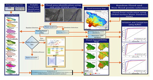
Graphical Abstract

Keywords:

• Flood susceptibility modeling
• machine learning algorithm
• Karnali River Basin
• Nepal

1. Introduction

A flood is the quick flow of a huge water volume for a brief period beyond the holding capacity of the river channel (Pangali Sharma et al. 2019; Andaryani et al. 2021). Floods are one of the most frequent and common natural disasters worldwide, causing devastating effects on human lives, physical infrastructures, societal welfare, and the economic status of the affected regions (UNDRR 2019; Diaconu et al. 2021). Climate change has led to an increase in flood magnitudes and occurrences, which has further exacerbated the damages caused by floods (Hirabayashi et al. 2013; Winsemius et al. 2016; Tabari 2020; Alifu et al. 2022). It is estimated that climate change and population growth in flood-prone areas, the exposure of the people and economy to floods is likely to increase by three factors (Merz et al. 2021).

Nepal, home to over 6000 rivers and rivulets with a total length of around 45,000 km, relies heavily on them for agriculture and livelihood (Gaire et al. 2015; Gupta et al. 2021). However, the high drainage density of 0.3 km/km² and restraining drainage capacity, and frequent flash floods (Rentschler et al. 2022) make these rivers prone to overflowing and causing damage (Dixit 2011; MoHA 2019; UNDRR 2019; Dingle et al. 2020; Rai et al. 2020; Thapa et al. 2020; Shrestha et al. 2020). Furthermore, due to the concentration of heavy rainfall events in a few months of monsoon, these rivers can cause significant flood disasters, affecting a large proportion of the livelihoods (Dingle et al. 2020). Floods annually cause several deaths and major economic damage to the country (MoHA 2018; UNDRR 2019; Shrestha et al. 2020), posing an imminent threat to human lives, physical infrastructures, societal welfare, and the economic status of developing countries like Nepal (Rai et al. 2020; Thapa et al. 2020). In fact, the loss due to floods in Nepal is expected to be 82.93% of the annual loss to the country (UNDRR 2019).

To mitigate the severity of flood hazards, proper watershed management is crucial (Andaryani et al. 2021). Preparing a flood susceptibility map (FSM) is an important component in making informed decisions regarding flood hazards (Youssef et al. 2022). An FSM is a binary classification that predicts whether a pixel will experience a flood (1) or not (0) based on past flood data and conditioning factors (Dodangeh et al. 2020; Nachappa et al. 2020). A range of physical, statistical, and decision-making methods are used for FSM, including hydraulic/hydrologic modeling, bivariate analysis, and the analytical hierarchy process (Khosravi, Pourghasemi, et al. 2016; Chakraborty and Mukhopadhyay 2019; Costache et al. 2020; Araujo and Dias 2021). However, each of these methods has its limitations. Less availability of various hydro-geomorphological observation data and the issue of data reliability and availability hinder the application of physically based models (Mosavi et al. 2018; Khosravi et al. 2020; Mehravar et al. 2023) and numerical modeling (Antwi-Agyakwa et al. 2023) in some regions (Khosravi et al. 2020; Liu et al. 2021; Seydi et al. 2023). Moreover, the physical models are affected by computational complexities and the proper selection of parameters (Fu et al. 2020). In recent years, the use of multi-criteria decision-making methods in FSM has gained popularity. However, the reliance on expert judgment in these methods can create biases, and even slight changes in parameter weights can have a significant impact on the results (de Brito et al. 2019; Ali et al. 2020; Mehravar et al. 2023). On the other hand, statistical methods such as frequency ratio (Tehrany et al. 2014; Shafapour Tehrany et al. 2017) and logistic regression models are widely used in flood modeling. However, these methods are based on linear assumptions and may not capture the non-linear behavior of floods (Pangali Sharma et al. 2019; Khosravi et al. 2020; Andaryani et al. 2021). The hydrological/hydraulic-based models use the non-linearity concept for their performance however, the geomorphological and environmental factors could factors affect their accuracies (Seydi et al. 2023). For basins larger than 1000 km², accurate two or three-dimensional analysis using a hydrodynamic model such as HECRAS is not feasible (Khosravi et al. 2020).

To overcome the limitations of traditional models, Machine Learning (ML) algorithms have been introduced, which utilize information based on the data provided without predefined assumptions or understanding of the physical process (Nachappa et al. 2020; Mishra et al. 2022) and help in rapid spatial data analysis (Dodangeh et al. 2020; Mishra et al. 2022). Some of the ML methods commonly used in FSM include artificial neural networks (ANN) (Tehrany et al. 2014; Shafapour Tehrany et al. 2017; Andaryani et al. 2021), support vector machines (SVM) (Yousefi et al. 2018; Li et al. 2019; Costache et al. 2020; Nachappa et al. 2020), gradient boosting (Ghosh et al. 2022; Seydi et al. 2023) and random forest (RF) (Schmidt et al. 2020; Nachappa et al. 2020). The Key steps in ML for FSM include analyzing the problem, preparing data, identifying a data-driven model, finding the best model, and evaluating it. Data-driven model identification is crucial, and minimizing the discrepancy between actual and predicted data during training achieves the best model approximation (Fu et al. 2020; Shahabi et al. 2020). Besides these ML-based modeling approaches deep learning models have shown great potential in various applications, but they are complex and demand a large training dataset to achieve high accuracy. These models have many hyperparameters, and tuning them can be difficult and time-consuming (Seydi et al. 2023). These approaches have led to the development of state-of-the-art ML models at different scales in FSM (Rahmati et al. 2020).

Similarly, in the context of flood risk management in Nepal, the application of machine learning (ML) models is limited. There have been studies using Gaussian process regression and SVM (Baig et al. 2022; Shreevastav et al. 2022) and MaxEnt (Shreevastav et al. 2022) in the Koshi Basin and a part of the Bagmati Basin respectively. However, most of the previous studies have focused on hydrodynamic analysis for flood modeling in the Karnali River Basin (KRB) and other river basins (MacClune et al. 2014; Aryal et al. 2020; Dingle et al. 2020; Rai et al. 2020). The potential of ML-based models such as support vector machines (SVM), random forests (RF), and artificial neural networks (ANN) for flood risk management is less explored in large river basins of Nepal.

To address the limitations of existing models used in FSM and the lack of data in larger river basins of Nepal, we focused on developing a simple yet effective and robust FSM for these basins. We propose an ML-based model for flood risk management in the KRB, a large river basin located in the southern slope area of the Himalayas. The KRB has a history of devastating floods, including the once-in-1000-year occurrence of mid-August 2014, which claimed the lives of 222 people and significantly impacted 120,000 more (MacClune et al. 2014; Aryal et al. 2020). The Terai portion of the KRB is particularly vulnerable due to broad and flat plains that contain more sediment deposits and unstable steep, rugged slopes that are raising the beds of the Karnali River by 10 to 30 cm per year (Team (NCVST) 2009; MacClune et al. 2014). These raised beds have resulted in the lowering of the elevations of several communities below the river, making them vulnerable to frequent floods (Dhakal 2013; MacClune et al. 2014). While early warning systems have helped to reduce the impact of floods to some extent (MacClune et al. 2014), our proposed ML-based model for flood risk management in the KRB has the potential to further improve decision-making processes in flood plain management. We aim to select the best ML approach among SVM, RF, and ANN, considering the influence of flood conditioning factors on the modeling approach. The proposed approach will generate a flood susceptibility map for the KRB, highlighting the area most susceptible to flood and the factors that contribute the most to the flood. Our study contributes to the national disaster risk reduction strategic plan of Action (2018–2030) (MoHA 2019; UNDRR 2019) based on the Sendai Framework for Disaster Risk Reduction (United Nations 2015), which aims to reduce the impact of natural disasters in Nepal.

2. Study area

Nepal is a landlocked-mountainous country lying in the central Himalayan region of southern Asia, situated between 80°4′E and 88°12′E longitude and 26°12′N to 30°27′N latitude (Talchabhadel et al. 2018; Pangali Sharma et al. 2019; Thapa et al. 2020). Extending 885 km and 140–250 km in the east-west and north-south regions. Nepal has diverse topography, ranging from 60 m in the southern plains to 8848.6 m of Mount Everest in the north. The study area of this project is Karnali River Basin , considered the longest river in Nepal (Figure 1) with a basin area of more than 46,000 km². Majorly snow-fed by glaciers with 1361 glaciers present over an area of 1740 km² (Ives et al. 2010) the KRB is composed of six major watersheds; Kawadi, West Seti, Humla Karnali, Mugu Karnali, Tila, and Bheri (Rai et al. 2020). Karnali stretches from the Tibetan region of China to the southern part of India. Originating from the southern part of Mansarovar and Rookas lakes in the Tibetan region, Karnali enters Nepal from Khojarnath and leaves through Chisapaani (Khatiwada and Pandey 2019). Karnali River is gravel-bottomed and the flow of the water in the channel is controlled by the sediment deposits (MacClune et al. 2014). The land-use pattern of the KRB is dominated by snow/bare land in the upper portion, while forest and agriculture are in a presiding role in the lower portion (Khatakho et al. 2021). The temporal distribution of the precipitation in the KRB is influenced by the monsoon, where the highest precipitation of 290.40 mm is observed in July, and the lowest precipitation of 12.51 mm is observed in November (Khatakho et al. 2021).

Figure 1. Location of the Karnali River Basin showing sample points used for training of the models and photographs of flooded areas, (a) Rajapur (b) Bardiya (c) Surkhet (d) Joshipur (e) Bhajani (f) Tikapur (Sources: a. www.myrepublica.com, b. www.wionews.com, c. www.khabarhub.com, d. www.spotlightnepal.com, e. www.ekantipur.com, and f. www.onlineradionepal.com).

3. Methodology

The proposed method of FSM is divided into two major sections: (1) Flood inventory mapping for preparation; and (2) modeling the flood susceptibility using the conditioning factors. The main steps in the proposed method of FSM include (1) Data collection and Preparation; (2) Preparation of a flood inventory map for the selection of training data set; (3) Preparation for the layers in flood conditioning factors; (4) Multicollinearity and Pearson test to analyze the suitability and relative importance of the conditioning factor; (5) train and test the ANN, SVM, and RF models using the flood inventory data; (6) use Information gain ratio (IGR) and Cohen Kappa Score in Leave-one-at-a-time cross-validation (LOOCV) approach to determine the most influential flood conditioning factors; (7) preparation of the susceptibility maps separately for ANN, SVM, and RF and (8) validation and comparison of the ML Algorithms using the Area Under the Curve of Receiver Operating Characteristics (AUROC), accuracy, F1-score, and kappa scores. A generalized flowchart of the study is shown in Figure 2.

Figure 2. Flowchart of flood susceptibility modeling.

3.1. Data collection and data preparation

For the research work, we collected the required geospatial data from different sources for our research work. Specifically, we obtained long-term rainfall data (Fick and Hijmans 2017) from WorldClim, Lithological map (DMG 1994) from the Department of Mines and Geology, ASTER Global Digital Elevation Model (ASTER GDEM) produced by the Advanced Spaceborne Thermal Emission and Reflection Radiometer (ASTER) (NASA 2022) instrument on board the Terra satellite of 30 m spatial resolution from the United States Geological Survey (USGS) official website), and flood area locations from the national disaster risk reduction portal (NDRR portal), and news reports for the date and time of flood occurrences.

3.2. Preparation of flood inventory map and training data-set

The Disaster Risk Reduction portal of the Nepal Government (http://drrportal.gov.np/) was explored for the location of flood points estimation. We used the UN-Spider Google Earth Engine (GEE) code (https://code.earthengine.google.com/f5c2f984c053c8ea574bfcd4040d084e) after the identification of the critical areas to identify the flooded area. The detection of water change is achieved by using Sentinel-1 imagery in the GEE code. A comparison was made between the Sentinel-1 image of the flood occurrence date and a non-flooded day. We manually created random flood points by utilizing field knowledge about the flood-prone areas and comparing them with the flood raster obtained from GEE (Figure 3). Non-flood points were created by selecting areas where flooding was not observed or are unlikely based on their location, slope, or elevation. To verify the accuracy of these points, we conducted a visual inspection using water extent, change, and availability maps derived from the Global Surface Water Data set (Pekel et al. 2017; Tang et al. 2020) and the Normalized Difference Water Index (NDWI) obtained through Google Earth Engine using Landsat Image (USGS 2022).

Figure 3. A snippet of flood and non-flood points selection based on Sentinel-1 SAR images of (a) before and (b) after flood using GEE.

The equation for NDWI is (1) $$\mathrm{NDWI}=\frac{\mathrm{Green}\text{-}\mathrm{NIR}}{\mathrm{Green}+\mathrm{ }\mathrm{NIR}}$$(1) where Green and NIR are the green and near-infrared bands. Based on the suggestion by different researchers (Buitinck et al. 2013; Towfiqul Islam et al. 2021) the same number of flood and non-flood pixels with a total of 424 points were prepared from the flood inventory to avoid biases (Figure 3). To increase the performance and accuracy of the models, 15-fold cross-validation was applied to the training dataset for all approaches. Similarly, the flood data was divided into different train-test split sizes from 80–20% to 50–50% with a difference of 5% and a significance test of the average scores was performed using a one-way ANOVA test to determine F-test and p-value.

3.3. Flood conditioning factors

After analyzing their potential effects, we selected ten flood conditioning factors based on the physiography of the KRB. These factors included elevation, slope, aspect, curvature, lithology, rainfall, Stream Power Index (SPI), Topographic Wetness Index (TWI), Distance to River (DTR), and Normalized Difference Vegetation Index (NDVI).

Elevation plays a crucial role in determining the distribution of topography and vegetation within the catchment (Nachappa et al. 2020). Lower regions with low elevation are more susceptible to damage (Li et al. 2019). Slope affects water flow and discharge, with steeper gradients resulting in faster water movement and lower infiltration rates (Shafizadeh-Moghadam et al. 2018). Aspect determines the hydrologic characteristics of the basin, with northward slopes receiving higher rainfall due to reduced exposure to solar radiation (Andaryani et al. 2021)]. However, in the Nepal Himalayas, the northern side forms a rain-shadow area with minimal rainfall (Panthi et al. 2015).

Curvature influences flood susceptibility, where positive values indicate convex surfaces and negative values indicate concave surfaces (Shafizadeh-Moghadam et al. 2018). Areas with higher curvature have a lower probability of flooding (Liu et al. 2021; Mehravar et al. 2023). Rainfall acts as a trigger for flooding, and increased rainfall intensifies the potential for flood occurrences. SPI represents erosive power and surface runoff intensity in a specific location (Khosravi et al. 2019). TWI characterizes accumulated flow (Nachappa et al. 2020), while DTR measures proximity to the river (Janizadeh et al. 2019). NDVI indicates vegetation availability, with dense vegetation reducing inundation and weak or no vegetation increasing flood vulnerability (Askar et al. 2022). The NDVI, SPI, and TWI were calculated from DEM using Equations (2)(2) $$\mathrm{NDVI}=\frac{\mathrm{NIR}\text{-}\mathrm{RED}}{\mathrm{NIR}+\mathrm{RED}}$$(2) , (3)(3) $$\mathrm{SPI}\mathrm{ }=\mathrm{ }As\text{ * tan}\beta$$(3) , and (4)(4) $$\mathrm{TWI}=\ln \left(\frac{A_s}{\tan \beta }\right)$$(4) . (2) $$\mathrm{NDVI}=\frac{\mathrm{NIR}\text{-}\mathrm{RED}}{\mathrm{NIR}+\mathrm{RED}}$$(2) (3) $$\mathrm{SPI}\mathrm{ }=\mathrm{ }As\text{ * tan}\beta$$(3) (4) $$\mathrm{TWI}=\ln \left(\frac{A_s}{\tan \beta }\right)$$(4) where, NIR and RED are near-infrared and RED bands. $A_s$ is the specific catchment area and $\beta$ is the slope gradient.

We used QGIS to prepare the flood conditioning factors. Once the preparation of the flood conditioning factors was completed, we reclassified the prepared rasters to create classes for identifying the flood-prone zone. To perform the reclassification, we applied different methods based on previous studies (Chapi et al. 2017; Bui et al. 2018; Shahabi et al. 2020), including manual division, equal division, quantile division, and natural breaks division. In this study, the natural breaks method was used for the reclassification of elevation, slope, aspect, rainfall, and NDVI. The quantile division method was employed for reclassifying TWI, SPI, and DTR. For soil and curvature, we performed manual division during the reclassification process (see Table 1, Figure 4).

Figure 4. Flood conditioning factors (a) Aspect, (b) Curvature, (c) DTR, (d) Elevation, (e) NDVI, (f) Rainfall, (g) Slope, (h) SPI, (i) Soil, (j) TWI.

Table 1. Data used to prepare flood conditioning factors

Conditioning factors	Spatial resolution	Primary Data	Data Source
Slope	30m x 30m	DEM	ASTER(GDEM)^1
Aspect	30m x 30m	DEM	ASTER(GDEM)^1
Elevation	30m x 30m	DEM	ASTER(GDEM)^1
Curvature	30m x 30m	DEM	ASTER(GDEM)^1
SPI	30m x 30m	DEM	ASTER(GDEM)^1
TWI	30m x 30m	DEM	ASTER(GDEM)^1
Distance from the river	30m x 30m	DEM	ASTER(GDEM)^1
NDVI	30m x 30m	Landsat Image	USGS^2
Lithology	1:100000	Geological map	Department of Mines and Geology^3
Rainfall	1km x 1km	Meteorological data	Worldclim^4

¹ (NASA 2022)(Fick and Hijmans 2017)

² (Ihlen and Zanter 2019).

³ (DMG 1994).

⁴ (Fick and Hijmans 2017).

3.4. Multicollinearity test

Due to the existence of a high correlation between two parameters the multicollinearity problem occurs (Dodangeh et al. 2020; Towfiqul Islam et al. 2021). There are different methods of Multicollinearity analysis, however, the Pearson correlation coefficient and VIF are preferred in hazard mapping (Tehrany, Jones, et al. 2019). If the tolerance value is below 0.2 and the VIF value is above 5 or 10 (Arabameri et al. 2019; Rahman et al. 2019; Baig et al. 2022; Ghosh et al. 2022; Mehravar et al. 2023), it indicates that there is multicollinearity among the parameters. Similarly, the value of a Pearson correlation coefficient less than 0.8 or 0.7 is considered less likely for the existence of collinearity (Tehrany, Jones, et al. 2019; Shrestha 2020; Shreevastav et al. 2022).

3.5. Evaluation of the importance of the flood conditioning factor based on information gain ratio and leave-one-out cross validation (LOOCV)

Another research objective was to determine the most influential flood conditioning factors and explore which factors are significant while preparing the models. The suitability and importance of factors in the flood are crucial before the application of the modeling approaches (Towfiqul Islam et al. 2021). We applied the information gain ratio (IGR) (Mehravar et al. 2023) to assess the importance and suitability of the factors due easy application and effectiveness (Dodangeh et al. 2020). To determine the importance of the factors, we applied the LOOCV approach. First, all the parameters were utilized, and the Kappa score was recorded for each model. After that, each of the parameters was removed one by one, and respective Kappa scores were recorded for all the models.

3.6. Flood susceptibility model using ANN, RF, and SVM

We trained the models using the flood points data and a stacked raster file of conditioning factors for SVM, RF, and ANN with Sci-kit Learn (Pedregosa Fabian et al. 2011) and Keras (Chollet 2015). ANN is a common ML method that shows the correlation between input conditioning factors and output through multilayer perceptron with hidden and output neurons (Dtissibe et al. 2020). RF creates numerous models through bagging (Richman and Wüthrich 2020) and random feature selection, then combines the findings to generate samples and anticipate output based on polling (Towfiqul Islam et al. 2021). SVM is a supervised learning binary classifier that estimates functions using a linear or kernel function (Nachappa et al. 2020) via hyperplane formation and binary categorization of data points as +1 or −1 (Tehrany et al. 2014). The success of the model is determined by the kernel function used, which can be sigmoid, polynomial, radial basis, or linear (Choubin et al. 2019).

3.7. Validation and comparison of the models

In the ML algorithm for flood susceptibility, pixels that are correctly classified as positive i.e. flood pixels (P), or negative, that is, non-flood pixels (N) are True Positives (TP) or True Negatives (TN), respectively. Likewise, Flood pixels and non-flood pixels that are incorrectly identified are referred to as False Positives (FP) and False Negatives (FN) (Chakraborty and Mukhopadhyay 2019; Choubin et al. 2019). The probability of correctly identifying positive and negative instances is represented by the true positive rate and true negative rate respectively (Pourghasemi et al. 2020). In the Receiver Operating Curve (ROC), the X-axis displays the false positive rate (1-specificity) (Equation 5(5) $$\mathrm{Specificity}\left(\text{True\hspace{0.5em}Negative\hspace{0.5em}Rate}\right)=\frac{TN}{\left(TN+FP\right)}$$(5) ), while the Y-axis shows the true positive rate (Sensitivity) (Equation 6(6) $$\mathrm{Sensitivity}\mathrm{ }\left(\text{True Positive Rate}\right)=\frac{\mathrm{TP}}{(\mathrm{TP}+\mathrm{FN})}$$(6) ). (5) $$\mathrm{Specificity}\left(\text{True\hspace{0.5em}Negative\hspace{0.5em}Rate}\right)=\frac{TN}{\left(TN+FP\right)}$$(5) (6) $$\mathrm{Sensitivity}\mathrm{ }\left(\text{True Positive Rate}\right)=\frac{\mathrm{TP}}{(\mathrm{TP}+\mathrm{FN})}$$(6) (7) $$\mathrm{Precision}=\frac{\mathrm{TP}}{\left(\mathrm{TP}+\mathrm{FP}\right)}$$(7)

The Area Under Curve of ROC (AUROC) is determined as (8) $$\mathrm{AUROC}=\sum TP+\frac{\sum TN}{P}+N$$(8)

Generally, an AUROC (Equation 8(8) $$\mathrm{AUROC}=\sum TP+\frac{\sum TN}{P}+N$$(8) ) value ranging from 0.5 to 0.6 is considered as the incompetent model, 0.6 to 0.7 indicates a poorly performing model, 0.7 to 0.8 is considered a satisfactorily performing model, and a model having an AUROC value greater than 0.8 is considered as the best performing models (Chapi et al. 2017; Towfiqul Islam et al. 2021; Ranjgar et al. 2021). For the validation and effectiveness of the model success and prediction rate curves were constructed respectively for train and test data sets (Khosravi, Pourghasemi, et al. 2016; Shafapour Tehrany et al. 2017). We used AUROC for success and prediction rates to test the performance of the ML algorithms and to validate the models (Mojaddadi et al. 2017; Andaryani et al. 2021). Similarly, kappa coefficient, accuracy, F1-scores (Seydi et al. 2023), MSE, and RMSE (Nguyen 2022) values were also evaluated for accuracy assessment and model comparison.

4. Results and discussion

4.1. Flood inventory and training dataset

The One-way ANOVA test showed an F-value and p-value of 2.481 and 0.112, respectively. The result implies that the difference of average scores (Table 2) from the mean value is insignificant so the train-test split size has insignificant effects on the values of average scores. Hence as a common practice, a 70–30% split size was applied using a random selection process as in various studies (Khosravi, Pourghasemi, et al. 2016; Tehrany, Kumar, et al. 2019; Khosravi et al. 2020; Andaryani et al. 2021; Baig et al. 2022).

Table 2. Mean Score for different train-test split sizes

Test Size	80%-20%	75%-25%	70%-30%	65%-35%	60%-40%	55%-45%	50%-50%
ANN mean score	0.929	0.931	0.922	0.921	0.929	0.918	0.930
RF mean score	0.932	0.931	0.946	0.920	0.933	0.935	0.934
SVM mean score	0.935	0.928	0.932	0.927	0.945	0.927	0.930

4.2. Multicollinearity test

The results from the multicollinearity test show that the VIF values are less than 10 and the tolerance is higher than 0.1. This reveals that all ten flood conditioning factors do not have any collinearity problems for utilization in FSM. On the other hand, the correlation matrix shows the strength of the linear relationship between the conditioning factors and flood susceptibility. Among the factors, elevation (0.675), slope (0.530), NDVI (0.529) and curvature (0.453) have relatively high correlation values but are less than 0.8. This indicated that the multicollinearity does not exist between any of the factors and hence can be used for the FSM (Table 3).

Table 3. Assessment of flood conditioning factors based on multicollinearity, Pearson test and Information Gain Ratio (IGR).

Conditioning factors	Aspect	Curvature	Distance to river	Elevation	NDVI
Correlation (Pearson)	0.003	0.453	0.297	0.675	0.529
VIF	1.039	1.313	1.142	2.401	1.322
Tolerance	0.962	0.762	0.875	0.416	0.756
IGR	0.006	0.099	0.109	0.39	0.179
Conditioning factors	Rainfall	Slope	Soil layer	SPI	TWI
Correlation (Pearson)	0.158	0.530	0.307	0.513	0.293
VIF	1.071	3.495	1.367	3.441	1.291
Tolerance	0.934	0.286	0.731	0.291	0.775
IGR	0.205	0.155	0.194	0.178	0.191

4.3. Comparison of the parameters

Based on the result as shown in Table 3, elevation (0.390), rainfall (0.205), soil (0.194), and TWI (0.191) have higher IGR values, indicating they are more important for flooding compared to other factors. Similarly, NDVI is the most influencing factor based on Cohen Kappa Score in the LOOCV method. The Kappa Score dropped sharply for all models when the NDVI parameter was removed. Likewise, the removal of elevation, distance to the river (DTR), and rainfall also decreased the score in the SVM model (Figure 5a). Curvature and TWI were found equally significant in the ANN model (Figure 5b). However, no other parameter showed a significant decrease in the case of the random forest model (Figure 5c). Aspect seems to be a less important factor in cases of SVM and ANN models (Figure 5a, b).

Figure 5. Parameter evaluation based on Cohen Kappa Score using leave-one-out cross-validation (LOOCV) method for (a) Support Vector Machine, (b) Artificial Neural Network, and c) Random Forest.

Based on the IGR and LOOCV, we observed that elevation, NDVI, DTR, rainfall, curvature, and TWI are the major factors that influence flooding in KRB (Table 3 and Figure 5). This result was similar to previous studies such as (Khosravi, Nohani, et al. 2016; Chapi et al. 2017; Bui et al. 2018; Tehrany, Jones, et al. 2019) but shows high contrast with the results such as by (Bui et al. 2015; Rahman et al. 2019).

Naturally, a flood occurs in areas of relatively low elevation and slope as such in the previous studies (Tehrany, Pradhan, and Jebur 2015; Khosravi, Nohani, et al. 2016; Khosravi, Pourghasemi, et al. 2016; Bui et al. 2018; Talukdar et al. 2020). Loamy sand and clay are major soil types in the flood susceptible area of KRB. Similarly, major floods occurred in the southern plain of the basin where extreme rainfall frequency is higher compared to the northern mountainous region. The area has low vegetation, slope, curvature, and TWI (Figures 3 and 4). The Karnali River enters into a low-elevation, low-slope flat area with a slope ranging from 0 to 3 degrees and branches into two major channels Karnali and Bheri channels forming the river island (Rakhal et al. 2021). This is because the upper region of KRB confines the water flow within its banks, and abrupt changes in elevation or breaches in the bank cause water to spread over vast flat areas (Dhakal 2013; Rakhal et al. 2021). This fact is supported by the results from IGR and LOOCV in this FSM study. The study by Andaryani et al. (2021) shows a similar ranking of the influencing factors. Similar results were observed by other studies as well (Talukdar et al. 2020; Towfiqul Islam et al. 2021). There are some contrasts in the importance of the factors in the study (Bui et al. 2015; Khosravi, Nohani, et al. 2016; Khosravi et al. 2020). Another study shows that slope, SPI, geology, and altitude are important factors for flood susceptibility (Tehrany, Kumar, et al. 2019). Major of the previous research (Tehrany, Kumar, et al. 2019; Andaryani et al. 2021; Youssef et al. 2022) shows that elevation is the major factor in FSM. Besides these other factors might vary according to the nature of the river basin such as geomorphology, hydrology, and topography (Tehrany, Kumar, et al. 2019; Andaryani et al. 2021).

4.4. Flood susceptibility mapping

During the preparation of the flood susceptibility map of KRB , it was observed that the major portion lying in the upper portion was covered by vegetation and contained solid bedrock, which in turn confines the river and reduces the flood susceptible area as represented in Table 4 and Figures 6, 7. Flood susceptibility maps show that ANN predicted a very low susceptible area of 82.22% (38,762 km²), followed by SVM at 55.12% (25,985 km²) and RF at 54.76% (25,818 km²). Similarly, for moderate flood risk, the SVM model dominated at 7.68% (3621 km²), followed by RF and ANN at 5.94% (2799 km²) and 2.39% (1125 km²) %, respectively. For very high flood-susceptible areas ANN model showed the highest at 2.467% (1163 km²), followed by RF at 0.995 (469 km²) % and SVM at 0.828% (390 km²). The majority of the susceptible area was found in the lower portion of the basin (area denoted in Table 4 by the phrase "very high" and enlarged portion in Figure 6). This region lacks vegetation, and more areas are exposed to direct runoff. Also, in the lower region, elevation decreases rapidly. Due to the sudden drop in the elevation and lowered slope, the sediment deposition is backed by extreme floods (Yousefi et al. 2021). As seen in the enlarged portion of Figure 6a–c, the braided river pattern represents the more susceptible land in the lower Terai portion. This is the area where the slope is lowered to 3° due to sedimentation and with a braided river pattern where major flooding occurs (Rakhal et al. 2021). The riverbeds in numerous Terai rivers are increasing in height at a rate of 10–30 cm annually due to sedimentation (MacClune et al. 2014). Likewise, the possible impacts of floods in this region are relatively high due to the development of cities with high population density such as Tikapur, Rajapur, Madhuwan, etc. (Aryal et al. 2020).

Figure 6. Flood susceptibility maps: (a) Support Vector Machine (b) Random Forest (c) Artificial Neural Network.

Figure 7. Flood susceptible areas in percentage obtained from Support Vector Machine, Random Forest, and Artificial Neural Network.

Table 4. Flood susceptible area (km²) predicted by support vector machine, random forest, and artificial neural network.

Flood	ANN	SVM	RF
Very low	38762	25985	25818
Low	5251	15378	16349
Moderate	1125	3621	2799
High	844	1771	1710
Very high	1163	390	469

4.5. Validation and comparison between different machine learning algorithms

The comparison between different ML algorithms was performed based on the AUROC, as shown in Figure 8 and Table 5. AUROC is one of the most reliable methods for the evaluation of predicted FSMs. The simplicity and easy understandability of the AUROC have made this popular in validations of spatial modeling (Nachappa et al. 2020; Andaryani et al. 2021; Youssef et al. 2022). From the results obtained, as represented inTable 5 and Figure 8, the SVM model performed better in comparison to RF and ANN. The SVM model exhibited superior performance, as evidenced by its highest AUROC value for both success and prediction rate with 92.8 and 98.7%, respectively, followed by RF (91.9 and 98.5%) and ANN (89.8 and 98.1%). Since the success is related to the fitting of the training data set so the prediction rate determines the applicability of the model (Tehrany, Pradhan, and Jebur 2015; Khosravi, Pourghasemi, et al. 2016; Andaryani et al. 2021). However, the results of AUROC for success and prediction are in line with each other so the results are consistent. Besides this, the accuracy, F1-score, and kappa scores of SVM were the highest among the models tested, with values of 0.953, 0.955, and 0.905, respectively, followed by RF (0.906, 0.930, and 0.809) and ANN (0.919, 0.923, and 0.795). Similarly, MSE and RMSE values are also lowest for SVM. These findings imply that the SVM model can deliver a more precise mapping of flood vulnerability, confirming its applicability in managing and planning floods. Because the SVM model offers a versatile and reliable method for modeling complicated interactions between climatic and topographical factors and flood occurrence, its application for FSM can be very beneficial similar to the studies by Tehrany, Pradhan, Mansor, et al. (2015) and Liu et al. (2021). The SVM model can simultaneously assess many features and data types, discover non-linear correlations between the predictors and the response variable, and detect subtle patterns and trends that other models might overlook (Tehrany, Pradhan, Mansor, et al. 2015; Tehrany, Kumar, et al. 2019). In the studies (Tehrany et al. 2014; Tehrany, Pradhan, and Jebur 2015), the results were compared between SVM and other statistical methods where SVM performed the best. The results are contrasting with the results from some researchers (Nachappa et al. 2020; Towfiqul Islam et al. 2021; Andaryani et al. 2021; Youssef et al. 2022; Seydi et al. 2023). The differences between the modeling approach in most of the indicators of the validation and comparison parameters are marginally different with values at the higher end. Therefore, while the SVM model demonstrated the best performance, the applicability of RF and ANN models cannot be ignored. The study aimed to propose a simple yet effective ML-based FSM for KRB. We found that the careful selection of the flood and non-flood points for the inventory preparation brought higher accuracy with SVM, RF, and ANN. The familiarity with the flood-prone areas in the KRB helped in creating better flood inventory which in turn helped in increasing the accuracy of the methods applied. Besides this, we believe that in the case of model validation use of statistical approaches might not be error-free (Meyer et al. 2019) so, the results from the models were compared by visual inspection to verify the prediction results and found appropriate. Likewise, the results were also compared with the flood hazard map from the Colorado flood observatory (https://floodobservatory.colorado.edu/) which includes the maximum flood extent from 1993. From the modeling approaches and visual inspection, a conclusion can be drawn that the flood susceptibility maps prepared from all three approaches are appropriate however, the result from SVM is more reliable.

Figure 8. Validation of FSM prediction rate and success rate curves for (a) ANN, (b) RF, and (c) SVM.

Table 5. Performance of models.

Methods	RF	SVM	ANN
True positive (TP)	50	54	52
True negative (TN)	66	68	63
False positive (FP)	5	3	8
False negative (FN)	7	3	5
Precision	0.924	0.949	0.923
Sensitivity	0.877	0.947	0.912
Specificity	0.930	0.958	0.887
MSE	0.101	0.094	0.094
RMSE	0.318	0.306	0.306
F1-Score	0.930	0.955	0.923
Accuracy	0.926	0.953	0.919
Kappa	0.809	0.905	0.795
AUROC (success rate)	0.919	0.928	0.898
AUROC (prediction rate)	0.985	0.987	0.981

5. Conclusions

The use of traditional approaches for FSM mostly the lack of data creates a major uncertainty and often relies on expert knowledge and field surveys, which can be time-consuming, expensive, and prone to errors. In contrast, ML models can be trained on historical data, which allows for the efficient analysis of large datasets, leading to faster and more accurate predictions. Besides this, the previous modeling approaches used fixed river channels. However, in KRB Periodic variations in the path of a river and the way sediment moves, which can change its physical shape and structure of the river channel and adjacent floodplain can modify the likelihood of flooding (Sinclair et al. 2017). For the preparation of the flood inventory historical flood data has been used in this study so the uncertainty due to channel shift is addressed. In the lower elevations of KRB, where morphological features from the bedrock gorge to the Indo-Gangetic plains create a favorable environment for floods, the research found highly susceptible areas. From various tests used in this study vegetation largely regulates the flood as the scores decreased for each model significantly when the NDVI parameter was removed, demonstrating the significance of vegetation in flood forecasts. Additionally, topographic factors like elevation and slope were found to play a critical role in runoff generation. The SVM model performed better than other models, as shown by the best AUROC precision, F1-score, and accuracy values whereas other models also performed well. This result signifies that the area of high flood risk area is in the range of 469 km² (from SVM) to 1163 km² (from ANN). We should thus like to reiterate that vegetation plays a vital role in flood control by increasing the flow path, and infiltration rates and decreasing the flow velocities and in many cases acts as a buffer zone against the settlements and flooding rivers. This should also be a part of floodplain management to protect people and property from floods. Hence, the results of this study should be useful to the state and local administrations and policymakers to develop effective flood management plans for KRB. It can be concluded that since floods continue to pose a significant threat to people and infrastructure worldwide, the application of ML models can play a crucial role in reducing the risks associated with flooding. With the development of advanced ML models and the increased computational power of information systems, accurate mapping tools are now available, allowing scientists to develop more accurate FSMs. These models are critical to developing viable and effective floodplain management strategies (Chen et al. 2019; Nachappa et al. 2020; Towfiqul Islam et al. 2021) and keeping people safe in flood-prone areas.

Data and Code Availability

The data and Jupyter Notebook (Python codes) that support the findings of this study are available on request in the Science Data Bank on https://www.scidb.cn/s/ueAzQf.

Acknowledgment

The authors would like to acknowledge the University Grants Commission, Nepal for providing a research grant. Similarly, the researcher would like to thank Yogesh Bhattarai, a research assistant at Khwopa College of Engineering, and Rocky Talchabhadel at Texas A&M AgriLife Research, Texas A&M University, USA for their help in data analysis and suggestions.

Disclosure Statement

The authors declare that they have no known competing financial interests or personal relationships that could have appeared to influence the work reported in this paper.

References

- Alifu H, Hirabayashi Y, Imada Y, Shiogama H. 2022. Enhancement of river flooding due to global warming. Sci Rep. 12(1):1–6.
- Ali SA, Parvin F, Pham QB, Vojtek M, Vojteková J, Costache R, Linh NTT, Nguyen HQ, Ahmad A, Ghorbani MA. 2020. GIS-based comparative assessment of flood susceptibility mapping using hybrid multi-criteria decision-making approach, naïve Bayes tree, bivariate statistics and logistic regression: a case of Topľa basin, Slovakia. Ecol Indic. 117(June):106620.
- Andaryani S, Nourani V, Haghighi AT, Keesstra S. 2021. Integration of hard and soft supervised machine learning for flood susceptibility mapping. J Environ Manage. 291(April):112731.
- Antwi-Agyakwa KT, Afenyo MK, Angnuureng DB. 2023. Know to predict, forecast to warn: a review of flood risk prediction tools. Water (Basel). 15(3):427.
- Arabameri A, Rezaei K, Cerdà A, Conoscenti C, Kalantari Z. 2019. A comparison of statistical methods and multi-criteria decision making to map flood hazard susceptibility in Northern Iran. Sci Total Environ. 660:443–458.
- Araujo JC, Dias FF. 2021. Multicriterial method of AHP analysis for the identification of coastal vulnerability regarding the rise of sea level: case study in Ilha Grande Bay, Rio de Janeiro, Brazil. Nat Hazards. 107(1):53–72.
- Aryal D, Wang L, Adhikari TR, Zhou J, Li X, Shrestha M, Wang Y, Chen D. 2020. A model-based flood hazard mapping on the southern slope of Himalaya. Water (Switzerland). 12(2):540.
- Askar S, Zeraat Peyma S, Yousef MM, Prodanova NA, Muda I, Elsahabi M, Hatamiafkoueieh J. 2022. Flood susceptibility mapping using remote sensing and integration of decision table classifier and metaheuristic algorithms. Water (Switzerland). 14(19):3062.
- Baig MA, Xiong D, Rahman M, Islam MM, Elbeltagi A, Yigez B, Rai DK, Tayab M, Dewan A. 2022. How do multiple kernel functions in machine learning algorithms improve precision in flood probability mapping? Nat Hazards. 113(3):1543–1562.
- de Brito MM, Almoradie A, Evers M. 2019. Spatially-explicit sensitivity and uncertainty analysis in a MCDA-based flood vulnerability model. Int J Geogr Inf Sci. 33(9):1788–1806.
- Bui DT, Khosravi K, Li S, Shahabi H, Panahi M, Singh VP, Chapi K, Shirzadi A, Panahi S, Chen W, et al. 2018. New hybrids of ANFIS with several optimization algorithms for flood susceptibility modeling. Water (Switzerland). 10(9):1210.
- Bui DT, Pradhan B, Revhaug I, Nguyen DB, Pham HV, Bui QN. 2015. A novel hybrid evidential belief function-based fuzzy logic model in spatial prediction of rainfall-induced shallow landslides in the Lang Son city area (Vietnam). Geomatics Nat Hazards Risk. 6(3):243–271.
- Buitinck L, Louppe G, Blondel M, Pedregosa F, Mueller A, Grisel O, Niculae V, Prettenhofer P, Gramfort A, Grobler J, et al. 2013. API design for machine learning software: experiences from the scikit-learn project, 1–15. http://arxiv.org/abs/1309.0238.
- Chakraborty S, Mukhopadhyay S. 2019. Assessing flood risk using analytical hierarchy process (AHP) and geographical information system (GIS): application in Coochbehar district of West Bengal, India. Nat Hazards. 99(1):247–274.
- Chapi K, Singh VP, Shirzadi A, Shahabi H, Bui DT, Pham BT, Khosravi K. 2017. A novel hybrid artificial intelligence approach for flood susceptibility assessment. Environ Modell Software. 95:229–245.
- Chen W, Hong H, Li S, Shahabi H, Wang Y, Wang X, Ahmad B. B. 2019. Flood susceptibility modelling using novel hybrid approach of reduced-error pruning trees with bagging and random subspace ensembles. J Hydrol (Amst). 575(February):864–873.
- Chollet F. 2015. Keras. GitHub. https://github.com/fchollet/keras.
- Choubin B, Moradi E, Golshan M, Adamowski J, Sajedi-Hosseini F, Mosavi A. 2019. An ensemble prediction of flood susceptibility using multivariate discriminant analysis, classification and regression trees, and support vector machines. Sci Total Environ. 651(Pt 2):2087–2096.
- Costache R, Popa MC, Tien Bui D, Diaconu DC, Ciubotaru N, Minea G, Pham QB. 2020. Spatial predicting of flood potential areas using novel hybridizations of fuzzy decision-making, bivariate statistics, and machine learning. J Hydrol (Amst). 585:124808.
- Dhakal S. 2013. Flood hazard in Nepal and new approach of risk reduction. Int J Landslide Environ. 1(1):13–14.
- Diaconu DC, Costache R, Popa MC. 2021. An overview of flood risk analysis methods. Water (Switzerland). 13(4):474.
- Dingle EH, Creed MJ, Sinclair HD, Gautam D, Gourmelen N, Borthwick AGL, Attal M. 2020. Dynamic flood topographies in the Terai region of Nepal. Earth Surf Process Landforms. 45(13):3092–3102.
- Dixit 2011. Climate Change in Nepal : Impacts and Adaptive. 1–8. www.worldresourcesreport.org/responses/climate-change-nepal-impacts-and-adaptive-strategies.
- DMG 1994. Geological Map of Nepal. https://www.dmg.gov.np/maps.
- Dodangeh E, Panahi M, Rezaie F, Lee S, Tien Bui D, Lee CW, Pradhan B. 2020. Novel hybrid intelligence models for flood-susceptibility prediction: meta optimization of the GMDH and SVR models with the genetic algorithm and harmony search. J Hydrol. 590(July):125423.
- Dtissibe FY, Ari AAA, Titouna C, Thiare O, Gueroui AM. 2020. Flood forecasting based on an artificial neural network scheme. Nat Hazards. 104(2):1211–1237.
- Fabian P, Michel V, Varoquaux G, Thirion B, Dubourg V, Passos A, Pedregosa V, Perrot M, Grisel Oliviergrisel O, Blondel M, et al. 2011. Scikit-learn: machine learning in Python. J Machine Learn Res. 12(Oct):2825–2830. http://scikit-learn.sourceforge.net.
- Fick SE, Hijmans RJ. 2017. WorldClim 2: new 1-km spatial resolution climate surfaces for global land areas. Int J Climatol. 37(12):4302–4315.
- Fu M, Fan T, Ding Z, Salih SQ, Al-Ansari N, Yaseen ZM. 2020. Deep learning data-intelligence model based on adjusted forecasting window scale: application in daily streamflow simulation. IEEE Access. 8:32632–32651.
- Gaire S, Delgado RC, González PA. 2015. Disaster risk profile and existing legal framework of Nepal: floods and landslides. Risk Manag Healthc Policy. 8:139–149.
- Ghosh S, Saha S, Bera B. 2022. Flood susceptibility zonation using advanced ensemble machine learning models within Himalayan foreland basin. Nat Hazards Res. 2(4):363–374.
- Gudiyangada Nachappa T, Tavakkoli Piralilou S, Gholamnia K, Ghorbanzadeh O, et al. 2020. Flood susceptibility mapping with machine learning, multi-criteria decision analysis and ensemble using Dempster Shafer Theory. J Hydrol (Amst). 590:125275.
- Gupta N, Dahal S, Kumar A, Kumar C, Kumar M, Maharjan A, Mishra D, Mohanty A, Navaraj A, Pandey S, et al. 2021. Rich water, poor people: potential for transboundary flood management between Nepal and India. Curr Res Environ Sustain. 3:100031.
- Hirabayashi Y, Mahendran R, Koirala S, Konoshima L, Yamazaki D, Watanabe S, Kim H, Kanae S. 2013. Global flood risk under climate change. Nat Clim Change. 3(9):816–821.
- Ihlen V, Zanter K. 2019. Landsat 8 (L8) Data Users Handbook. Department of the Interior, EROS, Sioux Falls, South Dakota: U.S. Geological Survey. Version 5, https://www.usgs.gov/media/files/landsat-8-data-users-handbook
- Ives JD, Shrestha RB, Mool PK. 2010. Formation of glacial lakes in the Hindu Kush-Himalayas and GLOF Risk Assessment. Kathmandu: Inernational Centre for Integrated Mountain Development (ICIMOD).
- Janizadeh S, Avand M, Jaafari A, Phong TV, Bayat M, Ahmadisharaf E, Prakash I, Pham BT, Lee S. 2019. Prediction success of machine learning methods for flash flood susceptibility mapping in the Tafresh watershed, Iran. Sustainability. 11(19):5426.
- Khatakho R, Talchabhadel R, Thapa BR. 2021. Evaluation of different precipitation inputs on streamflow simulation in Himalayan River basin. J Hydrol (Amst). 599(April):126390.
- Khatiwada KR, Pandey VP. 2019. Characterization of hydro-meteorological drought in Nepal Himalaya: a case of Karnali River Basin. Weather Clim Extrem. 26(November):100239.
- Khosravi K, Nohani E, Maroufinia E, Pourghasemi HR. 2016. A GIS-based flood susceptibility assessment and its mapping in Iran: a comparison between frequency ratio and weights-of-evidence bivariate statistical models with multi-criteria decision-making technique. Nat Hazards. 83(2):947–987.
- Khosravi K, Panahi M, Golkarian A, Keesstra SD, Saco PM, Bui DT, Lee S. 2020. Convolutional neural network approach for spatial prediction of flood hazard at national scale of Iran. J Hydrol (Amst). 591:125552.
- Khosravi K, Pourghasemi HR, Chapi K, Bahri M. 2016. Flash flood susceptibility analysis and its mapping using different bivariate models in Iran: a comparison between Shannon’s entropy, statistical index, and weighting factor models. Environ Monit Assess. 188(12):656.
- Khosravi K, Shahabi H, Pham BT, Adamowski J, Shirzadi A, Pradhan B, Dou J, Ly HB, Gróf G, Ho HL, et al. 2019. A comparative assessment of flood susceptibility modeling using multi-criteria decision-making analysis and machine learning methods. J Hydrol (Amst). 573(March):311–323.
- Liu J, Xiong J, Cheng W, Li Y, Cao Y, He Y. 2021. Assessment of flood susceptibility using support vector machine in the belt and road region. (May):1–37.
- Li X, Yan D, Wang K, Weng B, Qin T, Liu S. 2019. Flood risk assessment of global watersheds based on multiple machine learning models. Water (Switzerland). 11(8):1654.
- MacClune K, Venkateswaran K, ISET-International, Dixit KM, Yadav S, maharjan R, and Zurich Insurance GroupNepalKMKV, ISET-Nepal, Sumit Dugar, Practical Action Nepal. 2014. Risk Nexus Urgent case for recovery: what we can learn. Zurich: Zurich Insurance Company Ltd.
- Mehravar S, Razavi-Termeh SV, Moghimi A, Ranjgar B, Foroughnia F, Amani M. 2023. Flood susceptibility mapping using multi-temporal SAR imagery and novel integration of nature-inspired algorithms into support vector regression. J Hydrol (Amst). 617(PC):129100.
- Merz B, Blöschl G, Vorogushyn S, Dottori F, Aerts JCJH, Bates P, Bertola M, Kemter M, Kreibich H, Lall U, et al. 2021. Causes, impacts and patterns of disastrous river floods. Nat Rev Earth Environ. 2(9):592–609.
- Meyer H, Reudenbach C, Wöllauer S, Nauss T. 2019. Importance of spatial predictor variable selection in machine learning applications – Moving from data reproduction to spatial prediction. Ecol Modell. 411(March):108815.
- Mishra A, Mukherjee S, Merz B, Singh VP, Wright DB, Villarini G, Paul S, Kumar DN, Khedun CP, Niyogi D, et al. 2022. An overview of flood concepts, challenges, and future directions. J Hydrol Eng. 27(6):1–30.
- MoHA 2018. Ministry of Home Affairs, Disaster Risk Reduction National Strategic Plan of Action 2018–2030, Nepal.
- MoHA 2019. Nepal Disaster Report 2019. Kathmandu. http://drrportal.gov.np.
- Mojaddadi H, Pradhan B, Nampak H, Ahmad N, Ghazali A. b. 2017. Ensemble machine-learning-based geospatial approach for flood risk assessment using multi-sensor remote-sensing data and GIS. Geomat Nat Hazards Risk. 8(2):1080–1102.
- Mosavi A, Ozturk P, Chau KW. 2018. Flood prediction using machine learning models: literature review. Water (Switzerland). 10(11):1536.
- NASA. 2022. Aster Global Digital Elevation Model V003. National Aeronautics and Space Administration.
- Nguyen HD. 2022. Spatial modeling of flood hazard using machine learning and GIS in Ha Tinh province, Vietnam. J Water Climate Change. 14(1):200–222.
- Pangali Sharma TP, Zhang J, Koju UA, Zhang S, Bai Y, Suwal MK. 2019. Review of flood disaster studies in Nepal: a remote sensing perspective. Int J Disaster Risk Reduct. 34(9):18–27.
- Panthi J, Dahal P, Shrestha M, Aryal S, Krakauer N, Pradhanang S, Lakhankar T, Jha A, Sharma M, Karki R. 2015. Spatial and temporal variability of rainfall in the Gandaki River Basin of Nepal Himalaya. Climate. 3(1):210–226.
- Pekel J-F, Cottam A, Gorelick N, Belward A. 2017. Global Surface Water Explorer dataset.
- Pourghasemi HR, Kariminejad N, Amiri M, Edalat M, Zarafshar M, Blaschke T, Cerda A. 2020. Assessing and mapping multi-hazard risk susceptibility using a machine learning technique. Sci Rep. 10(1):1–11.
- Rahman M, Ningsheng C, Islam MM, Dewan A, Iqbal J, Washakh RMA, Shufeng T. 2019. Flood susceptibility assessment in Bangladesh using machine learning and multi-criteria decision analysis. Earth Syst Environ. 3(3):585–601.
- Rahmati O, Darabi H, Panahi M, Kalantari Z, Naghibi SA, Ferreira CSS, Kornejady A, Karimidastenaei Z, Mohammadi F, Stefanidis S, et al. 2020. Development of novel hybridized models for urban flood susceptibility mapping. Sci Rep. 10(1):1–19.
- Rai RK, van den Homberg MJC, Ghimire GP, McQuistan C. 2020. Cost-benefit analysis of flood early warning system in the Karnali River Basin of Nepal. Int J Disaster Risk Reduct. 47:101534.
- Rakhal B, Adhikari TR, Sharma S, Ghimire GR. 2021. Assessment of channel shifting of Karnali Megafan in Nepal using remote sensing and GIS. Ann GIS. 27(2):177–188.
- Ranjgar B, Razavi-Termeh SV, Foroughnia F, Sadeghi-Niaraki A, Perissin D. 2021. Land subsidence susceptibility mapping using persistent scatterer SAR interferometry technique and optimized hybrid machine learning algorithms. Remote Sens (Basel). 13(7):1326.
- Rentschler J, Salhab M, Jafino BA. 2022. Flood exposure and poverty in 188 countries. Nat Commun. 13(1):1–11.
- Richman R, Wüthrich M. v. 2020. Nagging predictors. Risks. 8(3):83.
- Schmidt L, Heße F, Attinger S, Kumar R. 2020. Challenges in applying machine learning models for hydrological inference: a case study for flooding events across Germany. Water Resour Res. 56(5):e2019WR025924.
- Seydi ST, Kanani-Sadat Y, Hasanlou M, Sahraei R, Chanussot J, Amani M. 2023. Comparison of machine learning algorithms for flood susceptibility mapping. Remote Sens (Basel). 15(1):192.
- Shafapour Tehrany M, Shabani F, Neamah Jebur M, Hong H, Chen W, Xie X. 2017. GIS-based spatial prediction of flood prone areas using standalone frequency ratio, logistic regression, weight of evidence and their ensemble techniques. Geomat Natural Hazards Risk. 8(2):1538–1561.
- Shafizadeh-Moghadam H, Valavi R, Shahabi H, Chapi K, Shirzadi A. 2018. Novel forecasting approaches using combination of machine learning and statistical models for flood susceptibility mapping. J Environ Manage. 217:1–11.
- Shahabi H, Shirzadi A, Ghaderi K, Omidvar E, Al-Ansari N, Clague JJ, Geertsema M, Khosravi K, Amini A, Bahrami S, et al. 2020. Flood detection and susceptibility mapping using Sentinel-1 remote sensing data and a machine learning approach: hybrid intelligence of bagging ensemble based on K-Nearest Neighbor classifier. Remote Sens (Basel). 12(2):266.
- Shreevastav BB, Tiwari KR, Mandal RA, Singh B. 2022. Flood risk modeling in southern Bagmati corridor, Nepal” (a study from Sarlahi and Rautahat, Nepal). Progress Disaster Sci. 16(November):100260.
- Shrestha BR, Rai RK, Marasini S. 2020. Review of flood hazards studies in Nepal. Geog Base. 7:24–32.
- Shrestha N. 2020. Detecting multicollinearity in regression analysis. AJAMS. 8(2):39–42.
- Sinclair HD, Brown S, Adhikari BR, Attal M, Borthwick A, Budimir M, Creed M, Dingle EH, Dugar S, Gautam D, et al. 2017. Improving understanding of flooding and resilience in the Terai, Nepal: 1–5. https://infohub.practicalaction.org/oknowledge/handle/11283/620609.
- Survey USG 2022. Landsat Level-1 data. https://www.usgs.gov/land-resources/nli/landsat.
- Tabari H. 2020. Climate change impact on flood and extreme precipitation increases with water availability. Sci Reports 10(1):1–10.
- Talchabhadel R, Karki R, Thapa BR, Maharjan M, Parajuli B. 2018. Spatio-temporal variability of extreme precipitation in Nepal. Int J Climatol. 38(11):4296–4313.
- Talukdar S, Ghose B, Shahfahad, Salam R, Mahato S, Pham QB, Linh NTT, Costache R, Avand M. 2020. Flood susceptibility modeling in Teesta River basin, Bangladesh using novel ensembles of bagging algorithms. Stoch Environ Res Risk Assess. 34(12):2277–2300.
- Tang X, Li J, Liu M, Liu W, Hong H. 2020. Flood susceptibility assessment based on a novel random Naïve Bayes method: A comparison between different factor discretization methods. Catena (Amst). 190(September):104536.
- Team (NCVST) NCVS 2009. Through the eyes of the vulnerability climate change induced uncertainties and Kathmandu.
- Tehrany MS, Jones S, Shabani F. 2019. Identifying the essential flood conditioning factors for flood prone area mapping using machine learning techniques. Catena (Amst). 175:174–192.
- Tehrany MS, Kumar L, Shabani F. 2019. A novel GIS-based ensemble technique for flood susceptibility mapping using evidential belief function and support vector machine: brisbane, Australia. PeerJ. 7:e7653.
- Tehrany MS, Pradhan B, Jebur MN. 2014. Flood susceptibility mapping using a novel ensemble weights-of-evidence and support vector machine models in GIS. J Hydrol (Amst). 512:332–343.
- Tehrany MS, Pradhan B, Jebur MN. 2015. Flood susceptibility analysis and its verification using a novel ensemble support vector machine and frequency ratio method. Stoch Environ Res Risk Assess. 29(4):1149–1165.
- Tehrany MS, Pradhan B, Mansor S, Ahmad N. 2015. Flood susceptibility assessment using GIS-based support vector machine model with different kernel types. Catena (Amst). 125:91–101.
- Thapa S, Shrestha A, Lamichhane S, Adhikari R, Gautam D. 2020. Catchment-scale flood hazard mapping and flood vulnerability analysis of residential buildings: the case of Khando River in eastern Nepal. J Hydrol: Reg Stud. 30:100704.
- Towfiqul Islam ARM, Talukdar S, Mahato S, Kundu S, Eibek KU, Pham QB, Kuriqi A, Linh NTT. 2021. Flood susceptibility modelling using advanced ensemble machine learning models. Geosci Front. 12(3):101075.
- UNDRR 2019. Disaster risk reduction in Nepal. Bangkok: UN Office for Disaster Risk Reduction and Asian Disaster Prevention Center.
- United Nations 2015. Sendai Framework for Disaster Risk Reduction 2015-2030. 69th session of the General Assembly. World Conference on Natural Disaster Reduction. 08955(June):24. http://www.un.org/en/development/desa/population/migration/generalassembly/docs/globalcompact/A_RES_69_283.pdf.
- Winsemius HC, Aerts JCJH, Van Beek LPH, Bierkens MFP, Bouwman A, Jongman B, Kwadijk JCJ, Ligtvoet W, Lucas PL, Van Vuuren DP, et al. 2016. Global drivers of future river flood risk. Nature Clim Change. 6(4):381–385.
- Yousefi S, Mirzaee S, Keesstra S, Surian N, Pourghasemi HR, Zakizadeh HR, Tabibian S. 2018. Effects of an extreme flood on river morphology (case study: Karoon River, Iran). Geomorphology. 304:30–39.
- Yousefi S, Pourghasemi HR, Rahmati O, Keesstra S, Emami SN, Hooke J. 2021. Geomorphological change detection of an urban meander loop caused by an extreme flood using remote sensing and bathymetry measurements (a case study of Karoon River, Iran). J Hydrol (Amst). 597:125712.
- Youssef AM, Pradhan B, Dikshit A, Mahdi AM. 2022. Comparative study of convolutional neural network (CNN) and support vector machine (SVM) for flood susceptibility mapping: a case study at Ras Gharib, Red Sea, Egypt. Geocarto Int. 37(26):11088–11115.