Multi-temporal InSAR and Sentinel-1 for assessing land surface movement of Joshimath town, India

Abstract

This study deals with the spatio-temporal measurement of land movement in Joshimath town using multi-temporal SBAS-InSAR technique. A network of 424 small-baseline interferograms was generated using 111 Sentinel-1 images acquired during May 2019–April 2023. Spatial distribution of line of sight displacement (LOSD) shows south-eastern Pekamarwadi, southern Gandhinagar and central Sunil wards are majorly affected; Manoharbagh, Singhdhar, and Lowerbazar moderately affected; northern Ravigram minor affected; and Parsari ward has no sign of land movement during investigation period. The observed negative values of mean LOS velocity and acceleration in southern Gandhinagar and central Sunil indicate these patchy areas are still susceptible and riskier for land stability. The SBAS-InSAR results were validated with CORS data during January 2022–March 2023. Trends show the gradual increase in LOSD from January to November 2022, rapid increase started from November 2022 and nearly ended mid January 2023, which indicates the initiation of movement stabilization. Accuracy assessment was performed in terms of Nash–Sutcliffe efficiency coefficient (NSE), $R^2,$ RMSE, and MAE, and the estimated values are 0.9896, 0.9495, 1.7534 cm, and 1.4028 cm, respectively. The analysis supports that CORS and SBAS-InSAR observed LOSD are in good agreement and reveals the true story of the land movement of Joshimath.

Keywords:

• Multi-temporal InSAR
• InSAR corrections
• time-series domain
• LOS displacement
• mean LOS velocity
• mean LOS acceleration

1. Introduction

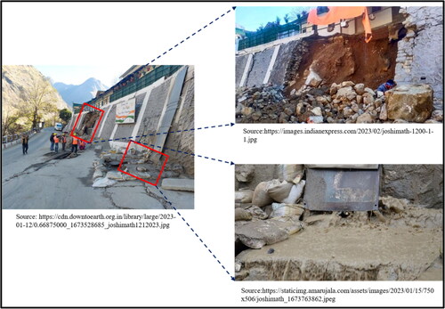
Seismically and ecologically, the north-west Himalayan region of Uttarakhand state is very sensitive. Therefore, the ecosystem is very fragile and always remains hazard prone, even after a slight disruption triggers a change that speedily resulted into a large-scale disaster in the region. Moreover, in recent times, developmental activities such as the construction of highways, high rise buildings and hydropower plants in the region have affected the wealth of local floras and faunas (Taloor et al. 2022). Rampant unplanned building construction and drainage is causing land instability in the Himalayan towns and could potentially cause more such incidents in near future. Although there is a long history of hazards in the region, but in the recent past in the first week of January 2023, there was a nationwide news of huge building cracks and land movement in Joshimath town in Chamoli district of Uttarakhand state. In the night of 2–3 January 2023, the deep cracks in many buildings with varying degree of damage appeared and few building walls collapsed in Joshimath town at many places. Local residents reported such incidents to the local administration and sooner it became a larger news head of national media. Consequently, it gripped fear amongst the residents and visitors of the place. District administration has taken proactive step to save the affected families. The unsafe buildings timely vacated as a precautionary measure in the entire town of Joshimath. After few days, the muddy water from suspected underground channel was spurting out near roadside wall of J.P. Colony in Pekamarwadi ward (Figure 1), and fluctuation in the percolated muddy water was observed for almost a week of time, and stopped slowly subsequently.

Figure 1. Muddy water spurting out near J.P. Colony in Pekamarwadi area from a unknown source.

On 10 January 2023, Government of Uttarakhand prepared a plan to demolish two multi-storey hotels (Malari Inn and Mount View) acutely affected by land movement in Joshimath. More than 650 buildings out of ∼2200 buildings were marked as ‘unsafe’. Most vulnerable buildings in the town are located at more than 30° terrain slope. The entire government machinery including the officials of National and State disaster response forces, district and state administration were involved in the rescue and relief operation. Multi-institutional team of experts of central and state government were involved in the damage assessment of vulnerable buildings. Apart from government institutions, the event had sparked global scientific interest with several groups of scientists, perusing satellite imagery as well as some teams making field visits to the town to assess the main cause of the land subsidence crisis. Several experts have given the name of this event differently such as land subsidence, land sinking, land slipping, land instability, land movement, land sliding etc. In this study, we used the term land movement for this event in Joshimath town. Officials of national disaster management authority (NDMA), Uttarakhand state disaster management authority, district administration of Chamoli reviewed the situation of Joshimath land crisis along with the experts of central and state governments. A comprehensive plan was also prepared to provide compensation to the owners of affected buildings and land pieces in terms of construction of new houses at new stable and safe locations, retrofitting of less damaged buildings etc. Government also promoting to the local residents to construct synthetic or semi-synthetic houses of comparatively smaller load in the town for sustainability.

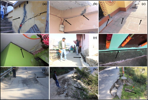
We visited Joshimath for field survey during in March–April 2022 and the cracks were observed in the buildings as shown in Figure 2. The survey was carried out rigorously in the Upperbazar, Lowerbazar, Gandhinagar, Pekamarwadi, Ravigram, Manoharbagh and Singhdhar wards out of nine wards of Joshimath. In several meetings during the visit, local residents told us that the cracks in the buildings were started developing after one to two months of Raini flash flood event of 7 February 2021. In Raini flash flood event, a vast amount of material consisting of rocks, muddy water, glacieret ice blocks, etc. was moving in the Rishiganga river valley of Garhwal Himalaya (NDMA 2022). This event took a record level of glacial debris flow in the downstream river valley of Rishiganga, and Dhauliganga towards Joshimath, and led to the toe cutting of the Dhauliganga and Alaknanda near Joshimath town. During the field survey, we observed that the cracks in parts of Gandhigram, Pekamarwadi, Manoharbagh and Singhdhar wards, were comparatively larger than that of Lowerbazar, Ravigram and Upperbazar areas. At few places, the cracks around 4–5 cm wide were appeared between wall and roof, and foundation and floor in residential buildings as shown in Figure 1(d–f). Road sections at different locations in the town were also appeared subsided along the down slope Figure 1(g–i).

Figure 2. Field photographs of March–April 2022 – (a) building in Ravigram, (b) building in Lowerbazar, (c) community health centre building in Gandhinagar, (d) building in Pekamarwadi, (e-f) building in Singhdhar, (g) a subsided road section of NH-7 in Pekamarwadi, (h–i) road sections in Singhdhar.

In the past three decades, multi-temporal interferometric synthetic aperture radar (MT-InSAR) techniques have been meticulously developed for detection, measuring and continuously monitoring of land surface deformation (Tough et al. 1995; Berardino et al. 2002; Ferretti et al. 2011; Guarnieri and Tebaldini 2007; Shankar et al. 2021, 2022). MT-InSAR has potential to derive the spatial and temporal progression of land surface deformation from a series of recurring SAR images. MT-InSAR measured accuracy of surface displacement time-series (D-TS) are limited mainly due to uncorrelated SAR signals, signal delays while propagating through atmosphere and errors in unwrapping the phase. Change of backscattering behaviour from incoherent targets over time and imperfect acquisition strategy of SAR systems are the main source of signal decorrelation. Several researchers have developed two advanced sets of MT-InSAR time-series techniques – (i) Permanent scatterer (PS) interferometry methods, that work on the selected phase stable pixels and are widely used over artificial infrastructures (Ferretti et al. 2001; Hooper et al. 2004); and (ii) Distributed scatterer (DS) interferometry methods, which slightly relaxed the harsh criteria of phase permanency of pixels and covered areas with decorrelation effect through the adjustment of multi-connected interferogram network. Based on the network of interferograms, DS methods are further divided into two categories – (i) in first category, a network of interferograms with shorter spatial and temporal baselines is used, called Small BAseline Subset (SBAS) (Berardino et al. 2002; Mora et al. 2003). In these methods, least squares method (LSM) with Lp-norm minimization is applied to solve the system of linear observation equations (Lauknes et al. 2011; Kim et al. 2023). If the interferogram network is not fully connected, singular value decomposition (SVD) or a regularization constraint (López-Quiroz et al. 2009) can be applied to find out the feasible solution, and (ii) second category of DS methods uses fully connected network of interferograms (Ferretti et al. 2011). The maximum likelihood estimator for highest precision (Guarnieri and Tebaldini 2007), or covariance matrix based eigenvalue decomposition can be applied for suboptimal solution of phase estimation (Samiei-Esfahany et al. 2016; Ansari et al. 2018). Although the second category of DS methods based on full network of interferograms, have ability to estimate the phase on areas with low coherence, but they show computational inefficiency compared to first category of methods. In both the methods, the sequence of processing steps can be swapped like network inversion pre-performed with phase unwrapping step to obtain the optimal phases. This study emphasizes the algorithmic efficiency, and implementation of first category of DS methods i.e. SBAS method with weighted least squares (WLS) estimator and linear deformation optimization (Yunjun et al. 2019).

Here we present a comprehensive land deformation analysis of Joshimath town in spatial and temporal domain using advanced SBAS-InSAR technique and freely available Sentinel-1 SAR datasets. The main objective of this study are – (i) utilization of free and open source computational environment for InSAR processing, (ii) inversion of raw phase time-series (P-TS) from small baseline interfrogram network, (iii) optimal phase correction in time-series domain rather than traditional interferogram domain, (iv) estimation of displacement time-series, velocity and acceleration to understand the kinematics of the region, and (v) validation of InSAR time-series results with the GNSS data.

2. Study region

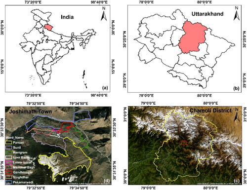
Joshimath town situated on the Rishikesh-Badrinath national highway-7 in Chamoli district of Uttarakhand is taken as the study site for this research as shown in Figure 3. The geographical extent of the study site lies between 30.535° N − 30.59° N and 79.52° E − 79.60° E, and the elevation ranges from 1200 to 3500 m from the mean sea level. The total area under investigation was 56.45 sq. km. The town also known as a Holi tourist town as it serves an overnight stay for frequent pilgrims/tourists visiting Joshimath, Badrinath, Auli, Valley of Flowers, and Hemkund Sahib. Due to high demand of hotels for the accommodation of tourists, the town has been undergoing a substantial construction work, and thus the blasting or digging also started to remove large boulders. Administratively, Joshimath town has nine wards namely Parsari, Sunil, Ravigram, Upperbazar, Lowerbazar, Manoharbagh, Gandhinagar, Singhdhar, and Pekamarwadi. Joshimath town is not located on the main rocks but rather on a historic deposition of sand and stone slides. Spread rocks in the town are shielded with ancient landslide (Misra 1976) consisting of stone boulders, fragmented rocks, and soft soil of low load bearing capacity. These fragmented rocks are extremely weathered and have a poor cohesive bonding particularly in monsoon seasons.

Figure 3. Location of study area – (a) map of Indian states and union territories, (b) districts map of Uttarakhand state, (c) administrative boundary of Chamoli district, and (d) wards map of Joshimath town.

The topography of the study area is very rugged with steep slopes, and the region comprises of high peaks separated by narrow valleys. The region forms part of the Alaknanda catchment and is traversed by several important rivers systems such as Dhauliganga, Rishiganga Raunthi Gadhera and their tributaries. The soil in the study area is a very thin top most layer of earth’s crust, containing both younger alluvial and old alluvial soil. The over-all climate of the study region is humid-temperate in summer and dry-cold in winter. The region receives rainfall through summer monsoon (May–Sep) as well as western disturbance in winter (Nov–Feb). Uttarakhand state receives ∼79% of the total annual rainfall during monsoon season (Jun-Sep) only. The annual average rainfall of Uttarakhand is 1494 mm (NDMA 2022). Geologically, the study area belongs to the Joshimath Formation of Vaikrita group of Higher Himalayan Crystalline (HHC) belt. HHC is located between Munsiari thrust in the south and South Tibetan Detachment System (STDC) in the north, and contains two sub-belts –(i) Munsiari group belt in the lesser Himalayan crystalline in the lower margin, and (ii) Greater Himalayan sequence belt along upper margin bounded by Vaikrita thrust (Main central thrust) and the STDC in the lower and upper margins, respectively (Mukherjee et al. 2019). The over thrust Vaikrita group of high-grade metamorphic rocks contains three formations in structurally in increasing order: (i) lowermost Joshimath formation, (ii) the Suraithota formation, also called Pandukeshwar formation, and (iii) uppermost Bhapkund formation. The Joshimath formation comprises of garnet-kyanite-biotite-muscovite bearing schist, psammitic gneiss with pegmatite and a leucogranite.

3. Weighted least squares and assumptions

SBAS-InSAR process multiple interferograms which might have varying level of noise, atmospheric delays and geometric distortions. Treating all interferograms with equal weights during estimation process could results in inaccurate deformation estimation. Therefore, based on the quality of interferogram, there is a need to assign appropriate weight to each interferogram. WLS method assigns lower weights to interferograms with higher noise level or less reliable data or low coherence, and higher weights to those with lower noise or more reliable data or better coherence.

Assuming there are N number of SAR images with signal phases $\left({\varphi }_1,{\varphi }_2,\dots \dots ,{\varphi }_N\right)$ acquired in same imaging geometry and over same area at sequential times $\left(t_1,t_2,\dots \dots ,t_N\right),$ and M interferograms are generated using all images coregistered with a common super reference image. All interferograms corrected with earth curvature, topography and phase-unwrapping, are referred as a stack of unwrapped interferograms where the phase is not bounded to $\left[-\pi ,\pi \right]$ range. Subsequently, the inversion problem can be exhibited as a system of M linear observation equations with raw P-TS $\varphi ={\left[{\varphi }_2,\dots \dots ,{\varphi }_N\right]}^T$ as the vector of $\left(N-1\right)$ unknowns with super reference acquisition with time $t_1.$ The time-series $\varphi$ relates to the observed path difference along slant range distance between SAR antenna and ground target in each image pair, including all systematic phase components such as raw ground deformation, SET, TPD, orbital ramps, and TPR (inaccuracy in DEM). For each pixel, the functional inversion model is described as: (1) $$\mathrm{\Delta }\mathrm{\varphi }=\mathbf{A}\mathrm{\varphi }+{\text{Δϕ}}_{\mathrm{\epsilon }}$$(1)

Where $\mathrm{\Delta }\varphi ={\left[\mathrm{\Delta }{\varphi }_1,\mathrm{\Delta }{\varphi }_2,\dots \dots .,\mathrm{\Delta }{\varphi }_M\right]}^T$ is a vector of interferometric unwrapped phases. A is the $M\times (N-1)$ connectivity matrix or design matrix representing acquisition pairs for interferogram generation. Thus each row of matrix A indicates an interferogram and column represents all acquisitions except super reference acquisition. The elements of each row of matrix A consists of $\pm 1,$ and 0, where +1 for primary acquisition, −1 for secondary acquisition of respective interferogram and 0 for others. $\Delta {\varphi }_{\epsilon }={\left[\mathrm{\Delta }{\varphi }_{\epsilon 1},\mathrm{\Delta }{\varphi }_{\epsilon 2},\dots .,\mathrm{\Delta }{\varphi }_{\epsilon M}\right]}^T$ is a residual phase vector that does not fulfil zero phase closure condition of interferogram triplets (Falabella and Pepe 2022) as it is contribution of several factors such as decorrelation noise, phase change due to dielectric properties of targets, inconsistency of processing chain like coregistration, resampling errors, multilooking, filtering, and phase unwrapping. A full rank (well-posed) design matrix A corresponds to a fully connected network, the estimated $\mathrm{\varphi }$ can be considered as an balanced WLS inversion of an overdetermined linear system. The feasible solution of Equation (1)(1) $$\mathrm{\Delta }\mathrm{\varphi }=\mathbf{A}\mathrm{\varphi }+{\text{Δϕ}}_{\mathrm{\epsilon }}$$(1) can be obtained by minimizing the L2-norm of the vector of interferometric phase residual ${\text{Δϕ}}_{\mathrm{\epsilon }}$ as: (2) $$\widehat{\varphi }={\left({\mathit{A}}^T\mathit{W}\mathit{A}\right)}^{-1}{\mathit{A}}^T\mathit{W}\mathrm{\Delta }\varphi$$(2)

Where $\widehat{\varphi }$ is the estimated raw P-TS and W is a $M\times M$ diagonal weight matrix. The oddity (error) between the measured and actual value of raw P-TS is given as ${\widehat{\varphi }}_{\epsilon }=\varphi -\widehat{\varphi }$ which propagated from ${\text{Δϕ}}_{\mathrm{\epsilon }}$ through a network of interferogram.

The applied approach in this research has two implied generalizations – (i) we assume that the phase residual term $\Delta {\varphi }_{\epsilon }$ in Equation (1)(1) $$\mathrm{\Delta }\mathrm{\varphi }=\mathbf{A}\mathrm{\varphi }+{\text{Δϕ}}_{\mathrm{\epsilon }}$$(1) representing phase triplet model is either exactly zero or negligible while applying WLS method. This assumption might not hold as due to the temporal changes in scattering mechanisms, the phases in multi-looked interferograms triplets are not conservative, (ii) the spatial correlation of decorrelated noise pixels is not considered in the processing chain. This assumption is only effective when the spatial resolution matches with pixel spacing, and not applicable in urban areas with strong reflecting targets. Although there are many weight functions such as uniform, spatial coherence, phase variance, and nonparametric Fisher information matrix as described in Yunjun et al. (2019). In order to apply WLS method, the choice of weight function is crucial for better inversion results. We chose the inverse of phase variance as the weight function W, as it gives the better results (Yunjun et al. 2019) to invert the stack of interferograms. Theoretically, the optimum choice of weight function is the maximum practicable precision bounded by decorrelation of phase which is in this case the phase variance. The phase variance can be calculated by integrating the probability distribution function (PDF) of phase. The phase PDFs for DS and PS are described in Tough et al. (1995) and Rodriguez and Martin (1992), respectively. The difference of phase PDFs of DSs and PSs vanishes when large number of looks are applied.

4. Materials and methods

4.1. Materials used

The material used in this study is comprises of space borne SAR data, CORS data, field observations and computing environment.

4.1.1. Satellite data

The Sentinle-1 (C-band, $\lambda =5.6 cm$) SAR data is capable to provide images with temporal resolution of 12 days with single sensor and 6 days with twin sensors i.e. Sentinel-1A & 1B. Sentinel-1 images are largely affects the spatial coherence due to vegetation cover over hilly region but it maintains excellent temporal coherence compare to previous SAR sensors. In this study, we have used a stack of 97 Sentinel-1A and 14 Sentinel-1B complex images acquired in descending pass. 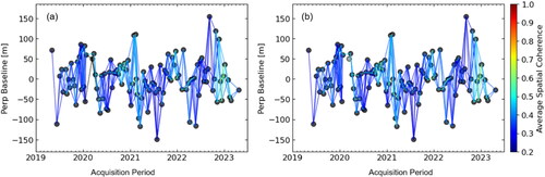A stack of 424 interferograms was generated with VV polarization, and $10\times 2$ looks along range and azimuth directions. Sentinel-1 images were downloaded from the Alaska Satellite Facility (URL: https://search.asf.alaska.edu/#/) for a period from 5 May 2019 to 26 April 2023. Sentinel-1 precise orbit files and SRTM DEM 1Sec HGT were downloaded from ESA Copernicus sentinels POD data hub (https://scihub.copernicus.eu/gnss/), and NASA's land processes distributed active archive centre (http://e4ftl01.cr.usgs.gov/MEASURES/SRTMGL1.003/), respectively. The study area is distress from low spatial coherence throughout the investigation period as Sentinel-1 interferograms are more easily to lose coherence and area is dominated with frequent precipitation. We selected interferometric pairs with small perpendicular baselines and temporal baselines of 226.85 m and 84 days, respectively. The selected scene having satellite heading angle of −167.22° and incidence angle ranging between 35.3° and 36.3° over the study area. The small baseline network before and after coherence-based network modification is shown in Figure 4.

Figure 4. Small baseline network – (a) before modification, and (b) after coherence-based network modification. Lines in (a) and (b) represent interferograms coloured by average spatial coherence. Gray circle in (b) represents the excluded SAR acquisition.

4.1.2. GPS data and field observation

The Continuously Operating Reference Stations (CORS) data i.e. GPS data was downloaded from the Survey of India website (https://www.cors.surveyofindia.gov.in/). In the study area, there is only one CORS with station code JOSH, continuously operating since January 2022. The geographical location of CORS is at 30°33′19.26848″N latitude, 79°33′29.07129″E longitude, and 1906.194 m elevation from mean sea level. The field observations were collected twice i.e. during 28 March − 1 April 2022 and April 2023.

4.1.3. Computing environment

In this study, the multi-temporal SBAS-InSAR processing was performed using completely free and open-source computational environment in an Ubuntu 20.4 Linux PC with 64 GB RAM, 2 TB hard disc and eight-core Intel64 CPU. The pre-processing of SAR data was done using well known and freely available InSAR Scientific Computing Environment (ISCE) SAR processor. The stable versions of ISCE package can be freely downloaded via GitHub (https://github.com/isce-framework/isce2) or it can be directly installed from conda-forge inventory (https://anaconda.org/conda-forge/isce2) using terminal command.

The main SBAS-InSAR time-series processing was performed using an open-source package called Miami INsar Time-series software in PYthon (MintPy). MintPy software is capable to read a coregistered and unwrapped stack of interferograms prepared by ISCE, ARIA-tools, FRInGE, HyP3, GMTSAR, SNAP, GAMMA or ROI_PAC SAR processors and produces spatio-temporal land surface deformation in radar line-of-sight (LOS) direction. MintPy software package can be freely downloaded from GitHub (https://github.com/insarlab/MintPy). One can also directly installed it from conda-forge inventory (https://anaconda.org/conda-forge/mintpy) using Linux terminal command. The entire MintPy processing including visualization of time-series deformation results was performed using Anaconda3 Jupyter Notebook. SNAPHU software package was used to unwrap coregistered stack of interferogram. SNAPHU software is freely available on http://web.stanford.edu/group/radar/softwareandlinks/sw/snaphu/ or it can be directly installed using Advanced Package Tool (APT). The QGIS software was used for map generation. All software packages used in this study are available on the web free of cost, and thus this approach of time-series deformation measurement is a cost-effective in comparison to other commercially available software such as SARscape, Gamma, SARPROZ etc.

4.2. Methods used

Current advancements of SBAS technique use various methods of tropospheric propagation delay (TPD) corrections to correct interferogram stack before inverting SBAS network. Moreover, the impact of TPD is deterministic in nature in InSAR observations, and it is preserved in the assessed phase time-series (P-TS). Analogous swapping of processing chain has also been applied to phase unwrapping (Guarnieri and Tebaldini 2008) and DEM error correction (Fattahi and Amelung 2015), and thus, the processing chain of SBAS allows phase corrections separation from network inversion (Pepe et al. 2011). In this study, a processing chain of SBAS-InSAR time-series analysis is applied with phase corrections in time-series rather than interferogram domain. Here the time-series domain indicates a series of phases chronologically sequenced in time with a common reference image, while in interferogram domain, the phases are arranged in acquisition pairs order. The entire time-series analysis was splitted into two parts (Pepe et al. 2011): (i) inversion of interferogram network for extracting raw P-TS, and (ii) separate solid earth tides (SET), TPD, orbital ramps, and topographic phase residual (TPR) from extracted raw P-TS to derive the corrected D-TS.

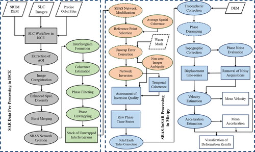
Based on processing stages, and data structures, the applied comprehensive methodology is divided into different blocks as shown in Figure 5: (a) Based on processing stages it divided into two blocks – (i) SAR pre-processing in ISCE, and (ii) SBAS-InSAR processing in MintPy; (b) Based on data structures, the processing workflow is divided into three blocks – (i) image domain, (ii) interferogram domain, and (iii) time-series domain.

Figure 5. Methodological processing workflow of SBAS-InSAR time-series analysis. Gray ovals and rectangle represents steps in image domain; green and orange ovals and rectangle represent steps in interferogram domain; blue ovals and rectangles show the steps in time-series domain; white rhombi and green rectangle show input data; blue and white rectangles output data; dashed boundaries represents optional steps.

4.2.1. Pre-processing of image stack

The methodological pre-processing workflow is shown by grey and green ovals and rectangles in Figure 5. First of all, SRTM DEM 1 Sec Hgt of vertical spatial resolution of 30 m, Sentinel-1 precise orbit files for each acquisition, and a series of SLC (level-1) images were downloaded as mentioned in section 4.1.1. Thereafter, a SLC workflow of ISCE package was opted to perform the SAR pre-processing and generating output compatible with MintPy package for executing main SBAS-InSAR processing. The pre-processing steps performed in ISCE are: (i) extraction of area of interest (AOI) in terms of sub-swath and bursts followed by selection of super reference image from a SLC image stack, and calculation of baselines in space and time; (ii) coregistration of secondary images with selected super reference image to generate a stack of all SLC images; (iii) improving spectral diversity and correcting phase shifts along range and azimuth directions; (iv) merge the bursts by interpolating the gap between successive bursts; (v) creation of multi-reference network (connections) controlled by a coherence threshold, maximum perpendicular and temporal baselines; (vi) generation of stack of interferograms and estimation of coherence (Rosen et al. 2012); (vii) low-pass phase filtering for smoothing the intensity of transformed samples and suppressing noise; (viii) unwrapping of interferogram stack.

4.2.2. SBAS-InSAR time-series processing workflow

In this study, we have implemented a MintPy workflow (Yunjun et al. 2019) in Jupyter Notebook for SBAS-InSAR time-series analysis using a stack of unwrapped interferograms processed in ISCE processor to derive D-TS as shown in right part of Figure 5. The processing workflow mainly provides two types of outputs: (a) unwrapping error correction and inversion of raw P-TS (orange ovals), and (b) estimation and removal of unwanted phase components to get the D-TS (blue ovals). The processing steps of SBAS-InSAR in MintPy are explained as-

4.2.2.1. Data loading and network modification

A coregistered stack of 424 unwrapped interferograms and estimated coherence, and pixel wise geometry files (DEM, incidence and azimuth angles) were loaded into MintPy environment. Subsequently, the multi-referenced SBAS network was modified for excluding the interferograms suffering from low coherence and causing unwrapping errors which deteriorate the accuracy of deformation results. Coherence-based network modification approach (Yunjun et al. 2019) was applied to modify the network, in which a minimum spanning tree (MST) network was created with inverse of average spatial coherence (ASC) as a weight function. Interferograms with ASC less than threshold value and not participating in MST network are excluded from the initial stack of unwrapped interferograms.

4.2.2.2. Spatial reference point selection

The selection of spatial reference point is important for many reasons such as referencing all interferograms to a common point in position, phase-unwrapping error corrections, inversion of SBAS network, and calculation of raw P-TS and D-TS etc. The spatial reference point was manually selected based on prior knowledge of the AOI and the following criteria was adopted in the selection – (i) point with high ASC to minimize decorrelation effect, (ii) point not much affected by strong atmospheric disturbance, (iii) point approximately at similar elevation as the AOI to reduce the effect of spatially correlated atmospheric delay, and (iv) located in non-deforming area. Since our study area under investigation is suffering from patchy deformation, therefore we manually selected a reference pixel on the south facing hilly rocky terrain (opposite to Joshimath town) which is stable and no sign of deformation is present, and having ASC of ∼0.8.

4.2.2.3. Correcting unwrapping errors

The interferometric phases are wrapped (modulo $2\pi$), and integration of wrapped phase (unwrapped phase), is required to obtain a field of relative phase with respect to a reference point in space. Interferometric phase noise and discontinuities among different coherent areas can lead to wrong $2\pi$ jumps when added to the phase and resulted as unwrapping error. The unwrapping errors were checked in terms of number of interferogram triplets with non-zero integer ambiguity $\left(T_{\mathit{int}}\right).$ The areas with $T_{\mathit{int}}>0$ indicates the unwrapping errors.

4.2.2.4. Network inversion

The network of M interferograms and N images was inverted using WLS method by minimizing L2-norm of the interferometric phase residual. The inverse of covariance was used as weight function for network inversion. It provided a raw P-TS for each acquisition except super reference acquisition. Temporal coherence was computed (Equation (3)(3) $${\gamma }_{\mathit{temp}}=\frac{1}{M}\left|{\mathit{H}}^T{e}^{j(\Delta \varphi -\mathit{A}\widehat{\varphi })}\right|$$(3) ) and temporal coherence mask was generated for pixels with reliable time-series estimation. (3) $${\gamma }_{\mathit{temp}}=\frac{1}{M}\left|{\mathit{H}}^T{e}^{j(\Delta \varphi -\mathit{A}\widehat{\varphi })}\right|$$(3)

Where H is a column vector of ones and order $M\times 1.$

The reliability of inverted raw P-TS for each pixel is assessed using the computed temporal coherence (Equation (3)(3) $${\gamma }_{\mathit{temp}}=\frac{1}{M}\left|{\mathit{H}}^T{e}^{j(\Delta \varphi -\mathit{A}\widehat{\varphi })}\right|$$(3) ) and number of interferogram triplets with $T_{\mathit{int}}\ne 0.$ Temporal coherence is considered as a potential ancillary measure for assessing the quality of inversion. High temporal coherence indicates the reliability of time-series with interferogram network.

4.2.2.5. Solid earth tides correction

The overall earth’s surface motion is determined by the many factors such as gravitational pull from the sun and the lunar (solid earth tides or SET); the procession motion of the earth’s rotational axis (polar tides); loading effect of ocean tides; atmospheric and hydrological loading; and land surface deformation prompted by plate tectonics, volcanic eruption, glacial melting, and anthropogenic activities (Yunjun et al. 2022). The SET displacement in the east-west, north-south, and up-down directions $\left[d_{ew}^{\mathit{set}},d_{ns}^{\mathit{set}},d_{ud}^{\mathit{set}}\right]$ was calculated using SET python wrapper with an accuracy of less than 1 mm and then projected to the radar LOS direction similar to Equation (11) (Yunjun et al. 2022).

4.2.2.6. Tropospheric delay correction and phase deramping

We corrected the tropospheric delays using an empirical linear relationship between the InSAR phase delay and topographic height (Doin et al. 2009) in the area. The more number of phase triplets help to mitigate the tropospheric artefacts that can affect the accuracy of deformation measurement. An extra multi-looking factor of 8 was applied to estimate the empirical phase to elevation ratio and to enhance the signal to noise ratio for tropospheric correction. Phase ramps are caused by residual atmospheric delays and orbital errors. Although, the removal of phase ramps is not required for long spatial wavelength deformation but in our case short spatial wavelength deformation signals were present and thus we estimated and removed the quadratic phase ramp from each time-series acquisition based on the phase of the reliable pixel.

4.2.2.7. Topographic correction

The systematic topographic phase residual caused by errors in the DEM, is estimated based on the proportionality with the perpendicular baseline time-series. For each pixel, the topographic residual (DEM error) can be estimated as (Yunjun et al. 2019). (4) $${\widehat{\varphi }}^i-{\widehat{\varphi }}_{\mathit{tropo}}^i=-\frac{4\pi }{\lambda }\left\{\frac{B_{\perp }^i}{r\mathrm{ }\sin \theta }{D}_{\epsilon }+\sum _{p=0}^n\frac{{\left(t_i-t_{sr}\right)}^p}{p!}{C}_p+\sum _{qϵI_s}H\left(t_i-t_q\right).B_q\right\}+{\varphi }_{\mathit{resi}}^i$$(4)

Where $t_i$ and $t_{sr}$ are the acquisition times of ith and super reference image; $B_{\perp }^i$ is the perpendicular baseline between $t_i$ and $t_{sr};$ r is the slant range distance between the radar antenna and ground target; θ is the incidence angle; $H\left(t_i-t_q\right)$ is a Heaviside step function centred at $t_q;$ $I_s$ is a set of indices describing offsets at specific prior selected times; $D_{\epsilon }, C_p$ and $B_q$ are the unknowns, which can be estimated using WLS by minimizing $L^2$-norm of residual P-TS ${\varphi }_{\mathit{resi}}={\left[{\varphi }_{\mathit{resi}}^1,{\varphi }_{\mathit{resi}}^2,\dots .,{\varphi }_{\mathit{resi}}^N\right]}^T.$ However, Equation (4)(4) $${\widehat{\varphi }}^i-{\widehat{\varphi }}_{\mathit{tropo}}^i=-\frac{4\pi }{\lambda }\left\{\frac{B_{\perp }^i}{r\mathrm{ }\sin \theta }{D}_{\epsilon }+\sum _{p=0}^n\frac{{\left(t_i-t_{sr}\right)}^p}{p!}{C}_p+\sum _{qϵI_s}H\left(t_i-t_q\right).B_q\right\}+{\varphi }_{\mathit{resi}}^i$$(4) offers the possibility to parameterize the geophysical processes using more complex models (Hetland et al. 2012).

4.2.2.8. Noise evaluation

The residual phase component ${\varphi }_{\mathit{resi}}^i$ (Equation (4)(4) $${\widehat{\varphi }}^i-{\widehat{\varphi }}_{\mathit{tropo}}^i=-\frac{4\pi }{\lambda }\left\{\frac{B_{\perp }^i}{r\mathrm{ }\sin \theta }{D}_{\epsilon }+\sum _{p=0}^n\frac{{\left(t_i-t_{sr}\right)}^p}{p!}{C}_p+\sum _{qϵI_s}H\left(t_i-t_q\right).B_q\right\}+{\varphi }_{\mathit{resi}}^i$$(4) ) can neither be corrected nor be modelled as land deformation, and thus, can only be used to quantify the noise level in the SBAS-InSAR time-series results. In this step, we compute the root mean square (RMS) of the residual phase ${\widehat{\varphi }}_{\mathit{resi}}$ for each acquisition as- (5) $${\mathit{RMS}}_{\mathit{resi}}^i=\sqrt{\frac{1}{N_{\omega }}\sum _{kϵ\omega }{\left(-\frac{\lambda }{4\pi }{\widehat{\varphi }}_{\mathit{resi}}^i\left(k\right)\right)}^2}\mathrm{ }$$(5)

Where ${\widehat{\varphi }}_{\mathit{resi}}^i(k)$ is the residual phase of ith acquisitionfor pixel k, $\omega$ is the set of reliable pixels after network inversion and $N_{\omega }$ is the total number of pixels to be inverted.

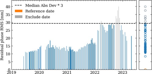
After computing RMS of residual phase for each acquisition, two tasks were performed – (i) identification of noisy SAR acquisitions with RMS detection threshold, and (ii) selection of optimal reference date corresponding to smallest RMS value. For identifying noisy acquisitions, we assumed that the residual tropospheric delay in residual phase is stochastic and normally distributed in time with zero-mean, and noisy acquisitions affected by severe atmospheric turbulence treated as outliers. The median absolute deviation (MAD) value was calculated and mark as a noisy acquisition if its RMS value (positive) is larger than the cut-off of +3 MAD. Moreover, the change of reference date at any moment during computation of velocity or acceleration does not change the numerical values of these estimators from the D-TS.

4.2.2.9. Estimation of LOS velocity and acceleration

In order to measure the rate of deformation, the first order time derivative of linear LOS D-TS i.e. mean LOS velocity $\left(v\right)$ was estimated from the slope of the best fitting linear curve (Equation (6)(6) $$-\frac{\lambda }{4\pi }{\varphi }_{\mathit{disp}}^i=v.t_i+c$$(6) ) to the D-TS graph. The mean LOS velocity (MLV) and its standard deviation ${(\sigma }_{\mathit{insar}}^v)$ were estimated as- (6) $$-\frac{\lambda }{4\pi }{\varphi }_{\mathit{disp}}^i=v.t_i+c$$(6) (7) $${\sigma }_{\mathit{insar}}^v=\sqrt{\frac{\sum _{i=1}^N{\left(d_i-{\widehat{d}}_i\right)}^2}{\left(N-2\right)\sum _{i=1}^N{\left(t_i-\overline{t}\right)}^2}}$$(7)

Where $i=1,2,\dots .,N$ is the number of images, and c is an unknown offset constant. $d_i$ and ${\widehat{d}}_i$ are the measured displacement and predicted displacement at time $t_i,$ and $\overline{t}$ is the average acquisition time.

The acceleration on estimation points (EPs) was estimated by the subtraction of the velocity of the subsequent observation date from the velocity of the penultimate observation date and dividing by the time. Assumption was made that the cluster of high acceleration point defines the general zone of instability on the north faced slope and thus will be the spot of land sinking. The SBAS-InSAR derived EPs point dataset was converted into a continuous acceleration image using inverse distance weighted interpolated method.

It is very important to notice that the values of default input parameters used in processing chain of MintPy do not always stand as a best choice and greatly affected by the characteristics of the study site and the deformation behaviour, and thus resulted into reduced quality of deformation. Therefore, for improved results within acceptable limits, the selection of input parameters in MintPy processing became a challenging task. In this study, for MintPy processing, the default values of input parameters in various steps were altered as shown in Table 1.

Table 1. Processing parameters used in different steps of MintPy processing.

Step	Method	Parameter	Used	Default
Modify_network	Coherence based	MinCoherence	0.22	0.7
Reference_point	Manual with high coherence	MinCoherence	0.80	0.85
		Spatial reference	30.574^0N, 79.56^0 E	NA
Correct_unwrap_error	Phase closure	NumSample	100	100
Invert_network	Weight function	Coherence	Coh	Var
		MaskThreshold	0.25	0.4
		MinRedundancy	1.0	1.0
		MinTempCoh	0.3	0.7
		MinNumPixel	100	100
Correct_troposphere	Height correlation	Looks	1	8
		PolyOrder	2	1
Deramp	Reliable pixels	Deramp	Quadratic	No
Correct_topography	Temporal deformation	PolyOrder	2	2
		StepFuncDate	No	No
Residual_RMS	Residual phase	Deramp	Quadratic	Quadratic
		Cut-off	3	3
Reference_date	Reference date	Date	20190505	20190505
Velocity	Velocity	Polynomial	1	1
		Periodic	1.0, 0.5	No
		StepDate	20230102	No
	Uncertainty	UncertaintyQuantification	Residue	Residue

4.2.3. Validation of SBAS-InSAR results

Global navigation satellite system provides positioning services with great-precision as the errors due to atmospheric delays, and clock offsets are mitigated in its design. CORS data derives the precise positioning in four dimensions (3D in space and 1D in time), and these positioning values can be used to derive horizontal and vertical components of actual displacement vector on the ground pixel. On the other side, the InSAR is a relative observation measurement technique in space and time, and measures displacement along the radar LOS. Therefore, in order to validate InSAR deformation results, the CORS measured 3D displacement vector needs to be projected along the radar LOS direction. The horizontal and vertical components of displacement vector measured by CORS were projected along the radar LOS direction corresponding to the InSAR acquisition moments (Yunjun et al. 2019) as - (8) $$d_{\mathit{los}}^{\mathit{gnss}}=\left[-\begin{array}{ccc}\hspace{0.17em}\sin \hspace{0.17em}\theta \sin \mu & \hspace{0.17em}\sin \hspace{0.17em}\theta \mathrm{ }\cos \mu & \hspace{0.17em}\cos \hspace{0.17em}\theta \end{array}\right].\left[\begin{array}{c}{d}_{ew}^g\\ d_{ns}^g\\ d_{ud}^g\end{array}\right]$$(8)

Where $d_{\mathit{los}}^{\mathit{gnss}}$ is the LOS displacement of CORS; ($\theta )$ is the radar incidence angle and ($\mu )$ is the azimuth look angle of satellite heading $\left(\alpha \right);$ $\begin{array}{ccc}{d}_{ew,}^g& d_{ns,}^g& and\mathrm{ }{d}_{ud}^g\end{array}$ are the three components of displacement vector along east–west, north–south and up–down directions, respectively.

Both SBAS-InSAR and CORS D-TS are referenced to a common date. The SBAS-InSAR data at CORS location was obtained by selecting the nearest geographical location of EP. The comparison of SBAS-InSAR and CORS D-TS was performed for a period from 1 January 2022–31 March 2023. Nash–Sutcliffe efficiency coefficient (NSE), coefficient of determination $\left(R^2\right),$ root mean square error (RMSE), and mean absolute error (MAE) were calculated for quantifying the accuracy of SBAS-InSAR results with CORS time-series as true value.

5. Results and discussion

We implemented the SBAS processing workflow outlined in section 4.2 to the Joshimath town of Chamoli district of Uttarakhand for the time-series measurement of land movement. Total eight interferograms were removed due to common size compatibility, and coherence based network modification removed six interferograms and one Sentinel-1 images from the interferogram stack and image stack, respectively.

5.1. Spatial and temporal coherence

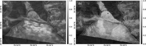
Coherence of SAR signals is very important in the reliability analysis of inverted time-series land deformation. The temporal coherence is the key indicator of reliability measure of SBAS network inverted raw P-TS results. In this study, the temporal coherence was obtained after inversion of coherence based modified SBAS network of interferograms using inverse variance weighting, and used to generate the mask of temporal coherence $\left(\ge 0.3\right)$ as a reliability measure of inverted results. The ASC (Figure 6(a)) and temporal coherence (Figure 6(b)) ranging between 0.2090–0.9010 and 0.0 − 1.0, respectively. The improved values of temporal coherence lead to identification of more reliable interferograms for further processing.

Figure 6. Distribution of coherence – (a) average spatial coherence, and (b) temporal coherence.

5.2. Network inversion and time-series phase corrections

In the traditional multi-temporal InSAR approaches, corrections in the unwanted phase components is applied in the interferogram domain but in this SBAS-InSAR approach we have applied these corrections in the time-series domain after network inversion. Both types of approaches give almost identical results (Yunjun et al. 2019), but the present approach has two main advantages over traditional interferogram domain approach – (i) computationally more efficient as it uses N-1 unwrapped phases rather than large number of interferograms, and (ii) The phase corrections are calculated and applied in both spatial and temporal domain.

The SBAS network was inverted using WLS estimator with covariance as weighting function. Figure 7(a) shows the raw cumulative LOS displacement (LOSD) varying between −29.62 − 12.76 cm. The unwrapped raw P-TS was corrected with the effect of SET (Figure 7(b)), and SET corrected displacement components were calculated and projected along radar LOS direction, and subtracted from the raw D-TS. The cumulative LOSD after SET correction is ranging from −28.96 − 12.79 cm. Delay of SAR signals due to spatio-temporal variation of atmosphere refractive index affects the quality of LOSD time-series (LOSD-TS) measurement. The stratified TPD was corrected using height correlation method (Doin et al. 2009), in which the extra multi-looking of 8 was applied to estimate the empirical phase to elevation ratio. In this way the existing dataset with 2 by 10 looks in azimuth and range was resulted into phase with 2*8 by 10*8 looks in azimuth and range directions, respectively. The resultant tropospherically corrected cumulative LOSD varying between −28.67 − 11.97 cm as shown in Figure 7(c).

Figure 7. Inverted cumulative LOSD with temporal reference to 5 May 2019 – (a) raw LOSD, (b) SET corrected LOSD, (c) stratified tropospheric delay corrected LOSD, (d) De-ramped LOSD, (e) topographic residual corrected LOSD, and (f) RMS of residual displacement. The black circle and black plus sign represent the location of CORS station and spatial reference point, respectively.

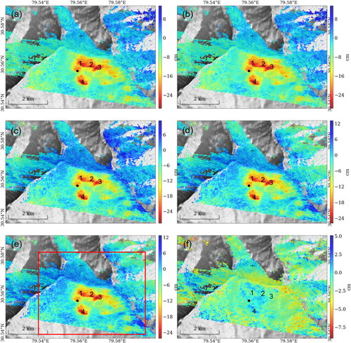
After correcting TPD correction, the raw P-TS were corrected for phase ramps partially generated by each atmospheric delays and orbital errors. Moreover, multi-temporal InSAR techniques use a series of SAR acquisitions, and thus most of the orbital errors are cancel out and not impacting the ability of the InSAR to derive deformation results. We have estimated and removed the quadratic phase ramp from each time-series acquisition based on the phase of the 17,206 reliable pixels. After derampping, the resultant cumulative LOSD was observed in the range of −25.91 − 13.07 cm as show in Figure 7(d). The acquisition date with minimum RMS value of residual phase was considered as a super reference acquisition. Subsequently, the TPR (DEM error) component was removed using SRTM DEM 1 arc second (∼ 30 m), second order temporal deformation model, and average phase velocity. The pixels with zero and nan values of incidence angle, slant range distance, and temporal coherence were removed during TPR correction, and total 46,768 pixels (58.9%) out of 79,411 pixels were inverted and corrected for TPR. The resultant cumulative LOSD was witnessed in the range of −26.20 − 12.80 cm (Figure 7(e)).

The residual phase component of Equation (4)(4) $${\widehat{\varphi }}^i-{\widehat{\varphi }}_{\mathit{tropo}}^i=-\frac{4\pi }{\lambda }\left\{\frac{B_{\perp }^i}{r\mathrm{ }\sin \theta }{D}_{\epsilon }+\sum _{p=0}^n\frac{{\left(t_i-t_{sr}\right)}^p}{p!}{C}_p+\sum _{qϵI_s}H\left(t_i-t_q\right).B_q\right\}+{\varphi }_{\mathit{resi}}^i$$(4) can neither be corrected nor be modelled as a land deformation, and can only be used to quantify the noise level of the InSAR time-series results. Thus, we calculate the root mean square (RMS) of residual phase for each acquisition as a quantification measure of InSAR LOSD-TS. The calculation was done over time-series residual phase with temporal coherence mask and RMS cut-off value of 29.2 mm which is 3.0 times MAD. Thus, 7 interferograms having RMS of residual phase more than 29.2 mm, were excluded during calculation of residual phase RMS as shown in Figure 8. The cumulative RMS value of residual P-TS is observing between −10.13 − 5.02 cm (Figure 7(f)).

Figure 8. RMS value of residual phase for noise evaluation.

Figure 9 shows the graphical representation of raw LOSD-TS and subsequent phase corrected LOSD-TS in sequential order such as SET, TPD, orbital ramps, and TPR corrections at four locations numbered as 1, 2, 3 and 4 (Figure 7) in the study area. At all four locations i.e. 1–4, the raw LOSD-TS (red lines) is varying between −20.94 − 0.26 cm, −19.97 − 0.0 cm, −17.62 − 0.0 cm, and −25.89 − 0.52 cm, respectively.

Figure 9. Correction of raw LOSD-TS at four point locations as shown in Figure 7.

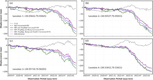
The SET corrected values (green dotted lines) are almost same with the raw LOSD-TS values at all respective locations which means the effect of SET due to gravitational pull of Sun and Moon is negligible in the study area. The tropospheric effect is observed largely and is in seasonal in nature, and the TPD corrected values (blue lines) are ranging from −18.41 − 0.38 cm, −18.34 − 0.15 cm, −15.27 − 0.43 cm, and −25.26 − 0.68 cm at locations 1–4, respectively. The time-series phase ramps and TPR (DEM Error) were estimated and the values of ramps corrections (solid black lines) are fluctuating between −16.26 − 0.75 cm, −16.10 − 0.50 cm, −13.52 − 0.75 cm, and −22.42 − 1.04 cm, and the DEM errors (magenta lines) are stretching from −16.52 − 0.39 cm, −16.4 − 0.0 cm, −13.73 − 0.37 cm, and −22.70 − 0.51 cm, respectively, at locations 1–4. The RMS value of residual P-TS for evaluating noise are calculated and the values are varying from −4.06 − 1.71 cm, −3.69 − 1.99 cm, −2.64 − 3.75 cm, and −3.13 − 3.75 cm, respectively, at locations 1–4.

5.3. Measurement of displacement, velocity and acceleration

The raw P-TS was corrected after applying SET, TPD, ramps, and TPR, and corrected cumulative raw P-TS was converted into cumulative LOSD in the study area. Figure 10 shows the spatial distribution of cumulative LOSD in the study area and its magnitude is varying between −26.20 − 12.80 cm during the investigation period (May 2019–April 2023). The negative values of cumulative LOSD denotes the land movement away from the satellite location. The higher negative values (red colour) of cumulative LOSD are observed in spatially distributed patches and these red patches show the downward land movement (away from satellite).

Figure 10. Cumulative LOS displacement overlaid with the wards boundaries. The black circle, plus sign and cross sign represents the locations of CORS station, spatial reference point and muddy water outlet, respectively.

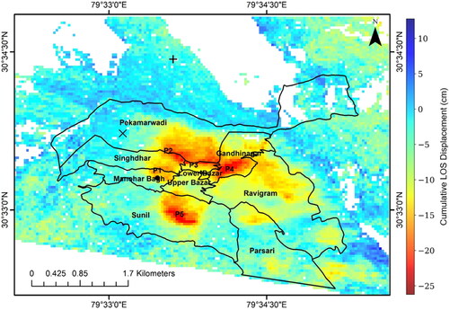
The red patches are lying in the central part of the Joshimath town and partially covering all wards except Parsari. The majorly affected wards (red coloured) by land movement are south-eastern Pekamarwadi, southern Gandhinagar and central Sunil wards in patched manner, while moderate affected wards (yellow coloured) are north-eastern Manoharbagh, eastern Singhdhar, central Lowerbazar, and northern Ravigram. At the location near J.P. colony (Figure 2) in Pekamarwadi ward shown by cross sign in Figure 10, the InSAR derived cumulative LOSD is very small and numerically varying between −5.0 and 0.0 cm during the entire investigation period. Moreover, when we visited the location in March–April 2022 and April 2023, there was no indication of physical damage/cracks in the infrastructure in and around the targeted location from where a sudden spurting of muddy water was seen in the first week of January 2023. Thus, both InSAR and field observations reflecting same conclusion at this location in J.P. colony.

Figure 11 shows the cumulative LOSD-TS plots at five different point locations P1–P5 (Figure 10) for a period from May 2019 to April 2023 where first acquisition was taken as a reference date. Points P1–P5 are situated at north-eastern corner of Manoharbagh, southern part of Pekamarwadi towards Singhdhar, northern side of Lowerbazar, southern part of Gandhinagar, and central part of Sunil wards, respectively. In the first week of January 2023, suddenly land movement and cracks in the buildings increased in Joshimath town and attracted the focus of many state and central agencies including central media. Keeping ground situation in mind, we have specifically extracted the LOSD at six different dates of investigation period i.e. 1 January 2022, 8 January 2023, and last four estimations on 1 February 2023, 13 February 2023, 25 February 2023, and 26 April 2023.

Figure 11. Cumulative LOS displacement time-series.

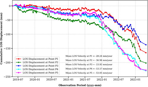
In general, the cumulative LOSD increasing slowly during May 2019 to January 2022, and increases rapidly from January 2022 to January–February 2023 at all the observation points (P1–P5) but in different magnitudes as shown in Figure 11. The cumulative LOSD of (−2.38 cm, −11.02 cm, −13.31 cm, −14.26 cm, −15.47 cm, −16.52 cm), (−7.77 cm, −16.41 cm, −17.79 cm, −18.47 cm, −19.43 cm, −20.18 cm), (−3.94 cm, −9.88 cm, −10.96 cm, −12.05 cm, −12.64 cm, −13.73 cm), (−6.15 cm, −19.87 cm, −20.88 cm, −21.71 cm, −22.28 cm, −22.88 cm), and (−6.76 cm, −21.19 cm, −21.57 cm, −21.91 cm, −22.24 cm, −22.70 cm) is estimated at points P1–P5 on 1 January 2022, 8 January 2023, 1 February 2023, 13 February 2023, 25 February 2023 and 26 April 2023, respectively. The LOSD deformation level at and around points P1 and P3 is of moderate order while that of at and around points P2, P4 and P5 is of severe order during the investigation period. These observations are also clearly indicating that the LOSD is increasing very slowly after January–February 2023 at all observations points P1–P5 which is almost equivalent to the stabilization of land movement in the study area. This may be because of many factors such as evacuation of residents of affected buildings, restrictions on travel of outside pilgrims in the town, the minimization of usage of domestic water after this event, etc. The magnitude of cumulative LOSD at points P4 and P5 is higher than that of points P1–P3, which means the InSAR observed land deformation is higher in southern part of Gandhinagar and central part of Sunil. Pekamarwadi ward is on third number, and Manoharbagh/Singhdhar and Lowerbazar are on fourth and fifth number. However, the Ravigram shows a small scale LOSD in its northern part and Parsari ward is a safe zone in term of land movement or instability.

The MLV and its standard deviation were estimated using linear regression (Equation (7)(7) $${\sigma }_{\mathit{insar}}^v=\sqrt{\frac{\sum _{i=1}^N{\left(d_i-{\widehat{d}}_i\right)}^2}{\left(N-2\right)\sum _{i=1}^N{\left(t_i-\overline{t}\right)}^2}}$$(7) ) over InSAR LOSD-TS results and (Equation (8)(8) $$d_{\mathit{los}}^{\mathit{gnss}}=\left[-\begin{array}{ccc}\hspace{0.17em}\sin \hspace{0.17em}\theta \sin \mu & \hspace{0.17em}\sin \hspace{0.17em}\theta \mathrm{ }\cos \mu & \hspace{0.17em}\cos \hspace{0.17em}\theta \end{array}\right].\left[\begin{array}{c}{d}_{ew}^g\\ d_{ns}^g\\ d_{ud}^g\end{array}\right]$$(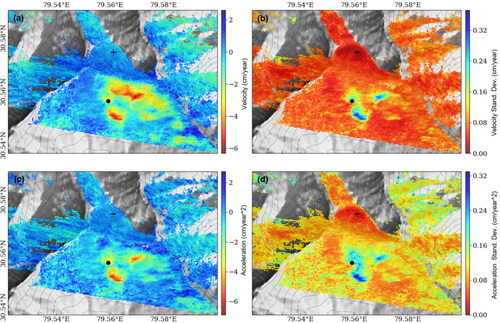8) ), respectively. The mean LOS acceleration (MLA) was estimated by the subtraction of the velocity of the subsequent observation date from the velocity of the penultimate observation date and dividing by the time. The estimated MLV, standard deviation of MLV, MLA and standard deviation of MLA are, respectively, shown in Figure 12(a–d). The MLV and MLA values with negative sign represents the movement away from the satellite sensor. The values of MLV, standard deviation of MLV, MLA and standard deviation of MLA in the study area are ranging between −6.32 cm/year to 2.54 cm/year), 0.0 cm/year to 0.37 cm/year, −6.91 cm/year² to 2.60 cm/year², and 0.0 cm/year² to 0.36 cm/year², respectively. The maximum negative values of MLV are observed in Pekamarwadi, Gandhinagar and Sunil wards. The maximum MLA values away from the satellite platform are observed in the small patches in the southern part of Gandhinagar and central part of Sunil wards. The negative values acceleration in these area Gandhinagar and Sunil wards indicates that the area still undergoing land movement (sinking zones) and is riskier area in terms of land stability.

Figure 12. Velocity and acceleration and their standard deviations.

5.4. Validation of SBAS-InSAR deformation results

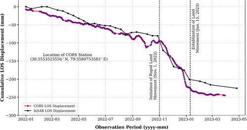
The cumulative LOSD-TS results measured from SBAS-InSAR technique were compared with the LOSD derived from CORS observations. The CORS derived LOSD was calculated using three components of displacement vector along east-west, north-south and up-down directions and Equation (9). In Joshimath town, SOI installed one CORS station in 2021 and it is continuously operating since January 2022. Figure 13 shows the time-series variation of CORS derived LOSD and SBAS-InSAR estimated LOSD versus observation period at the CORS location in Joshimath town. The CORS data was analysed for a period from 1 January 2022 to 31 March 2023 and the LOSD was calculated with reference to 1 January 2022. Similarly, the SBAS-InSAR LOSD was taken with reference to 1 January 2022. The trend of CORS derived LOSD shows the linear slow increase in LOSD from January–November 2022, and rapid increase started from November 2022 and nearly ended mid of January 2023, and thereafter becomes almost constant till the end of March 2023. The InSAR estimated LOSD follow the same trend as that of CORS derived LOSD but the values are slightly underestimated throughout the observation period as shown in Figure 13. Figure 13 very clearly shows that the rapid movement started from November 2022 but it was evidently observed by local residents in January 2023 when it crosses a threshold and became uncontrollable beyond the holding capacity of the infrastructure. This supports the finding of CORS LOSD and SBAS-InSAR estimated LOSD are in good agreement and reveals the true story of the land surface movement of Joshimath town.

Figure 13. Comparison of SBAS-InSAR estimated and CORS derived LOSD.

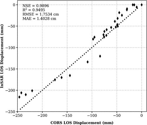
The accuracy assessment of LOSD-TS results retrieved from SBAS-InSAR was performed with respect to LOSD-TS of CORS in terms of NSE, R², RMSE and MAE. The 1:1 plot between CORS derived LOSD-TS (true data) versus SBAS-InSAR estimated LOSD-TD (measured data) at CORS locations is shown in Figure 14. The calculated values of NSE, R², RMSE and MAE between SBAS-InSAR and CORS LOSD-TS at CORS location are 0.9896, 0.9495, 1.7534 cm, and 1.4028 cm, respectively. These values of performance parameters very strongly indicate that the SBAS-InSAR deformation results are in good agreement with the CORS derived LOSD values. Thus, the applied SBAS-InSAR technique has performed better retrieved LOSD-TS results of Joshimath town.

Figure 14. Accuracy assessment of SBAS-InSAR results at CORS location.

Moreover, at the location in J.P. colony (Figure 2) from where the flow of muddy water from a suspected underground channel was observed in the first week of January 2023 and no physical damage in terms of cracks in surrounding buildings/infrastructure were observed before (field observation in March–April 2022), during (Figure 2) and after (field observation in April 2023) flow of muddy water. InSAR investigations also show very small range of deformation at the location marked by a cross sign in Figure 10, which indicates the good agreement between the field observations and InSAR results.

5.5. Probable causes

There are total six natural water drainage (nallas) flowing from top hills (Auli side) to the river side passing through the town. Over the period, these nallas are blocked by the unplanned construction activities in the town which enforce the accumulation and percolation of surface water (natural spring water, and domestic drinking and sewerage water) into sub-surface level. The presence of heavy boulders at sub-surface level also wires accumulation of percolated water at sub-surface level. This sub-surface accumulated water creates pressures on soft soil and flows downward along the slope through the soft soil in the form of muddy water which was also evident at certain locations during this event. This sub-surface flow of water with soft soil increases the chance of more land instability.

The topography of the study area is very rugged with steep slopes, and the region comprises of high peaks separated by narrow valleys. Moreover, the soil in the study area is the thin upper most layer of the earth’s crust, comprising mainly combination of younger alluvial and old alluvial soil. The alluvial soil of the area is dry, porous, sandy, faint yellow and consists of clay and organic matter. The thin soil layer is separated from hard rock at sub-surface level. The percolation of surface water into sub-surface loose and thin layer of soil along with steep slope creates a lubricant effect (weak cohesive forces) with hard rock at sub-surface level becomes main cause of land instability and slipping of land down the slope.

In the recent past, two earthquakes were occurred in the region - first on 11 September 2021 of magnitude 4.7 with epicentre in WNW hills near Pipalkoti and around 30 km from Joshimath, and second on 23 May 2021 of magnitude of 4.5 with epicentre in the NW of Joshimath at ∼45 km (Yang et al. 2023). The shock of these seismic events near Joshimath are also one of the causative factors of initiation and onset of land movement in the town.

The region has a long history of hazards events such as earthquake of magnitude >8 on the Richter scale (1803), flash flood with landslides (1893), cloudburst triggered flash flood (1970), earthquake of magnitude 6.8 on Richter scale (1999), landslides (2004), flash flood (2009), cloudburst resulting into flash flood (2013), glacial outburst flood (2021), and land subsidence/sinking (2023). Long hazard history of flash flood in the region activated the toe cutting (undercutting) by river currents of Alaknanda and Dhauliganga and playing important role in increasing land movement down the slope.

6. Conclusions

In this study, a very powerful technique of space borne radar remote sensing i.e. SBAS-InSAR is used to detect, measure and continuous spatio-temporal monitoring of land deformation of Joshimath town with an accuracy of few cm order. The inverted raw cumulative LOSD-TS is observed between −29.62 − 12.76 cm during May 2019–April 2023 with 5 May 2019 as a temporal reference. The SET, TPD, orbital ramps, and TPR corrected LOSD-TS are, respectively, estimated between −28.96 − 12.79 cm, −28.67 − 11.97 cm, −25.91 − 13.07 cm, and −26.20 − 12.8 cm. The corrected LOSD-TS observation show – (i) minimal effect of SET over the study area, (ii) the study area undergoes with a significant seasonal effect of atmospheric propagations delays during the investigation period. The cumulative RMS value of residual LOSD-TS is found between −10.13 − 5.02 cm.

The spatial distribution of land movement shows the major deformation affected (red patches) wards are south-eastern Pekamarwadi, southern Gandhinagar and central Sunil wards in patched manner, while moderate affected wards (yellow coloured) are north-eastern Manoharbagh, eastern Singhdhar, central Lowerbazar, and northern Ravigram, and Parsari has no sign of land deformation in Joshimath. Cumulative LOSD-TS plot at five different point locations P1–P5 shows the critical temporal observations at six different dates i.e. 1 January 2022, 8 January 2023, 1 February 2023, 13 February 2023, 25 February 2023, and 26 April 2023. In general, the cumulative LOSD is increasing slowly during May 2019 to January 2022, and increases rapidly from January 2022 to January–February 2023 at all the observation points (P1–P5) but in different magnitudes. These observations are also clearly indicating that the LOSD is increasing very slowly after January–February 2023 at all observations points P1–P5 which is almost equivalent to the stabilization of land movement in the town. The values of MLV, standard deviation of MLV, MLA and standard deviation of MLA in the study area are estimated between −6.32 − 2.54 cm/year, 0.0 − 0.37 cm/year, −6.91 − 2.60 cm/year², and 0.0 − 0.36 cm/year², respectively. The maximum negative values of MLV are observed in Pekamarwadi, Gandhinagar and Sunil wards while the maximum MLA values are observed in the small patch of southern part of Gandhinagar and central part of Sunil wards. The negative values acceleration in these area Gandhinagar and Sunil wards indicates that the area still showing movement and is riskier in near future.

The LOSD-TS results were validated with CORS data during January 2022–March 2023 at CORS location. The trend of CORS derived LOSD (Figure 13) shows the linear slow increase in LOSD from January to November 2022, and rapid increase started from November 2022 and nearly ended mid of January 2023, and thereafter becomes almost constant till the end of March 2023. The InSAR estimated LOSD follow the same trend as that of CORS derived LOSD. The accuracy assessment of LOSD-TS of SBAS-InSAR was performed with respect to that of CORS in terms of NSE, R², RMSE and MAE and the estimated values are 0.9896, 0.9495, 1.7534 cm, and 1.4028 cm, respectively. The analysis supports the finding of CORS LOSD and SBAS-InSAR estimated LOSD are in good agreement and reveals the true story of the land surface movement of Joshimath town of Uttarakhand.

Acknowledgement

In this research, we used the existing computing and infrastructural facilities of Indian Institute of Remote Sensing (IIRS), Dehradun, India. The authors are very thankful to – (i) Alaska Satellite Facility (URL: https://search.asf.alaska.edu/#/) for providing time-series dataset of Sentinel-1A&1B satellite, (ii) ESA’s Copernicus Sentinels POD Data Hub for providing Sentinel-1 precise orbit files, (iii) NASA’s Land Processes Distributed Active Archive Centre for proving SRTM DEM 1 ArcSec, (iv) Survey of India for providing CORS data.

Disclosure statement

No potential conflict of interest was reported by the author(s).

Additional information

Funding

This research did not receive any specific grant from any funding agency in the public, commercial, or not-for-profit sector.

References

- Ansari H, De Zan F, Bamler R. 2018. Efficient phase estimation for interferogram stacks. IEEE Trans Geosci Remote Sensing. 56(7):4109–4125. doi: 10.1109/TGRS.2018.2826045.
- Berardino P, Fornaro G, Lanari R, Sansosti E. 2002. A new algorithm for surface deformation monitoring based on small baseline differential SAR interferograms. IEEE Trans Geosci Remote Sensing. 40(11):2375–2383. doi: 10.1109/TGRS.2002.803792.
- Doin M-P, Lasserre C, Peltzer G, Cavalié O, Doubre C. 2009. Corrections of stratified tropospheric delays in SAR interferometry: validation with global atmospheric models. J Appl Geophys. 69(1):35–50. doi: 10.1016/j.jappgeo.2009.03.010.
- Falabella F, Pepe A. 2022. On the phase nonclosure of multilook SAR interferogram triplets. IEEE Trans Geosci Remote Sensing. 60:1–17. doi: 10.1109/TGRS.2022.3216083.
- Fattahi H, Amelung F. 2015. InSAR bias and uncertainty due to the systematic and stochastic tropospheric delay. J Geophys Res Solid Earth. 120(12):8758–8773. doi: 10.1002/2015JB012419.
- Ferretti A, Fumagalli A, Novali F, Prati C, Rocca F, Rucci A. 2011. A new algorithm for processing interferometric data-stacks: squeeSAR. IEEE Trans Geosci Remote Sensing. 49(9):3460–3470. doi: 10.1109/TGRS.2011.2124465.
- Ferretti A, Prati C, Rocca F. 2001. Permanent scatterers in SAR interferometry. IEEE Trans Geosci Remote Sensing. 39(1):8–20. doi: 10.1109/36.898661.
- Guarnieri AM, Tebaldini S. 2007. Hybrid CramÉr–Rao bounds for crustal displacement field estimators in SAR interferometry. IEEE Signal Process Lett. 14(12):1012–1015. doi: 10.1109/LSP.2007.904705.
- Guarnieri AM, Tebaldini S. 2008. On the exploitation of target statistics for SAR interferometry applications. IEEE Trans Geosci Remote Sensing. 46(11):3436–3443. doi: 10.1109/TGRS.2008.2001756.
- Hetland EA, Musé P, Simons M, Lin YN, Agram PS, DiCaprio CJ. 2012. Multiscale InSAR Time Series (MInTS) analysis of surface deformation: MULTISCALE INSAR TIME SERIES. J Geophys Res. 117(B2):n/a–n/a. doi: 10.1029/2011JB008731.
- Hooper A, Zebker H, Segall P, Kampes B. 2004. A new method for measuring deformation on volcanoes and other natural terrains using InSAR persistent scatterers: a NEW PERSISTENT SCATTERERS METHOD. Geophys Res Lett. 31(23):1–5. doi: 10.1029/2004GL021737.
- Kim J, Lin S-Y, Singh T, Singh RP. 2023. InSAR time series analysis to evaluate subsidence risk of monumental Chandigarh City (India) and surroundings. IEEE Trans Geosci Remote Sensing. 1–1. doi: 10.1109/TGRS.2023.3305863.
- Lauknes TR, Zebker HA, Larsen Y. 2011. InSAR deformation time series using an $L_{1}$-norm small-baseline approach. IEEE Trans Geosci Remote Sensing. 49(1):536–546. doi: 10.1109/TGRS.2010.2051951.
- López-Quiroz P, Doin M-P, Tupin F, Briole P, Nicolas J-M. 2009. Time series analysis of Mexico City subsidence constrained by radar interferometry. J Appl Geophys. 69(1):1–15. doi: 10.1016/j.jappgeo.2009.02.006.
- Misra MC. 1976. Commissioner Garhwal Mandal, high level committee report on Joshimath sinking. Dehradun, India: Government of Uttarakhand.
- Mora O, Mallorqui JJ, Broquetas A. 2003. Linear and nonlinear terrain deformation maps from a reduced set of interferometric SAR images. IEEE Trans Geosci Remote Sensing. 41(10):2243–2253. doi: 10.1109/TGRS.2003.814657.
- Mukherjee PK, Jain AK, Singhal S, Singha NB, Singh S, Kumud K, Seth P, Patel RC. 2019. U-Pb zircon ages and Sm-Nd isotopic characteristics of the Lesser and Great Himalayan sequences, Uttarakhand Himalaya, and their regional tectonic implications. Gondwana Res. 75:282–297. doi: 10.1016/j.gr.2019.06.001.
- NDMA. 2022. Detailed report: Uttarakhand disaster on 7th February 2021. New Delhi: NDMA, MHA, Govt. of India.
- Pepe A, Bertran Ortiz A, Lundgren PR, Rosen PA, Lanari R. 2011. The Stripmap–ScanSAR SBAS approach to fill gaps in Stripmap deformation time series with ScanSAR Data. IEEE Trans Geosci Remote Sensing. 49(12):4788–4804. doi: 10.1109/TGRS.2011.2167979.
- Rodriguez E, Martin JM. 1992. Theory and design of interferometric synthetic aperture radars. IEE Proc F Radar Signal Process UK. 139(2):147. doi: 10.1049/ip-f-2.1992.0018.
- Rosen PA, Gurrola EM, Sacco GF, Zebker H. 2012. The InSAR scientific computing environment, in synthetic aperture radar. Paper presented at: 9th European Conference on EUSAR; Apl 23–26; Nuremberg, Germany.
- Samiei-Esfahany S, Martins JE, van Leijen F, Hanssen RF. 2016. Phase estimation for distributed scatterers in InSAR stacks using integer least squares estimation. IEEE Trans Geosci Remote Sensing. 54(10):5671–5687. doi: 10.1109/TGRS.2016.2566604.
- Shankar H, Roy A, Chauhan P. 2021. Persistent scatterer interferometry for Pettimudi (India) landslide monitoring using Sentinel-1A images. Photogramm Eng Remote Sensing. 87(11):853–862. doi: 10.14358/PERS.21-00020R3.
- Shankar H, Singh D, Chauhan P. 2022. Landslide deformation and temporal prediction of slope failure in Himalayan terrain using PSInSAR and Sentinel-1 data. Adv Space Res. 70(12):3917–3931. doi: 10.1016/j.asr.2022.04.062.
- Taloor AK, Thapliyal A, Kimothi S, Kothyari GC, Gupta S. 2022. Geospatial technology-based monitoring of HAGL in the context of flash flood: a case study of Rishi Ganga Basin, India. Geosystems Geoenvironment. 1(3):100049. doi: 10.1016/j.geogeo.2022.100049.
- Tough RJA, Blacknell D, Quegan S. 1995. A statistical description of polarimetric and interferometric synthetic aperture radar data. Proc R Soc Lond Ser Math Phys Sci. 449:567–589. doi: 10.1098/rspa.1995.0059.
- Yang F, An Y, Ren C, Xu J, Li J, Li D, Peng Z. 2023. Monitoring and analysis of surface deformation in alpine valley areas based on multidimensional InSAR technology. Sci Rep. 13(1):12896. doi: 10.1038/s41598-023-39677-3.
- Yunjun Z, Fattahi H, Amelung F. 2019. Small baseline InSAR time series analysis: unwrapping error correction and noise reduction. Comput Geosci. 133:104331. doi: 10.1016/j.cageo.2019.104331.
- Yunjun Z, Fattahi H, Pi X, Rosen P, Simons M, Agram P, Aoki Y. 2022. Range geolocation accuracy of C-/L-band SAR and its implications for operational stack coregistration. IEEE Trans Geosci Remote Sensing. 60:1–19. doi: 10.1109/TGRS.2022.3168509.