A novel model for multi-risk ranking of buildings at city level based on open data: the test site of Rome, Italy

Abstract

In the context of population concentration in large cities, assessing the risks posed by geological hazards to enhance urban resilience is becoming increasingly important. This study introduces a robust and replicable procedure for assessing ground instability hazards and associated physical risks. Specifically, our comprehensive model integrates spatial hazard assessments, multi-satellite InSAR data, and physical features of the built environment to rank and prioritize assets facing multiple risks, with a focus on ground instabilities. The model generates risk scores based on hazard probability, potential damage, and displacement rates, aiding decision-makers in identifying high-risk buildings and implementing appropriate mitigation measures to reduce economic losses. The procedure was tested in Rome, Italy, where the analysis revealed that 60% of the examined buildings (90 × 10³) are at risk of ground instability. Specifically, 33%, 22%, and 5% exhibit the highest multi-risk score for sinkholes, landslides, and subsidence, respectively. Landslide risk prevails among residential structures, while retail and office buildings face a higher risk of subsidence and sinkholes. Notably, our study identified a positive correlation between mitigation expenses and the multi-risk scores of nearby buildings, highlighting the practical implications of our findings for urban planning and risk management strategies.

Keywords:

• Multi-risk
• ground instability hazards
• urban resilience
• data fusion
• InSAR
• open data

1. Introduction

Large cities often face natural and geological hazards, engineering geological, and technological threats. The importance of the analysis and evaluation of geo-hazards for effective risk mitigation measures is evident in view of implementing effective strategies to make our cities and communities more resilient to natural disasters (Frankenberg et al. 2013). Due to the increased incidence of extreme weather events and human-made hazards related to accelerated urban growth (UNISDR 2012), built-up areas are specifically threatened and should therefore be the priority target of the action. Identifying the spatial distribution and concentration of risks in urban areas helps determine where and how preventive and corrective actions can reduce levels of vulnerability and exposure of urban populations (Johnson et al. 2016). Therefore, simplified vulnerability and risk assessment methodologies have been gaining space and importance (Kappes et al. 2012a; Liu Z et al. 2015; Romão et al. 2016; Liu X and Chen 2019; Wei et al. 2022). Geo-hazards risk assessment provides strategic input for enhancing city resilience through mitigation design (McGlade et al. 2019). Nevertheless, losses from natural disasters continue to grow (White et al. 2001; Annual Report 2022). According to Kappes et al. (2012b), this may be due to a lack of interaction between science and practice in terms of knowledge transfer and applicability of results. To fill this gap, multi-risk assessment must support decision-makers by providing them with valuable information regarding the types and probabilities of hazards and their physical impacts, which will guide mitigation measures (Komendantova et al. 2014).

The statement that natural hazards almost never occur individually is of great importance: this leads to the notion of multi-risk (Gill et al. 2022). Multi-risk is generated from the presence of multiple hazards that may also be correlated, affecting the same elements exposed (Terzi et al. 2019). The interrelationships between these hazards and vulnerability level should be considered. A necessary condition for risk prevention, mitigation and reduction is its analysis, quantification, and assessment (Ward et al. 2020; Hochrainer-Stigler et al. 2023). However, assessing the risks and vulnerabilities of an entire city is a very demanding task, requiring considerable amount of data, technical knowledge and financial resources that are usually not available (Kappes et al. 2012b; van Westen et al. 2014; Julià and Ferreira 2021). Different temporal and spatial scales of hazardous events, and the potential interactions between hazards and socio-economic fragilities make multi-risk assessment problematic (Bell and Glade 2004; Kappes et al. 2012a). Existing risk assessment methods integrate large volumes of data and sophisticated analyses, as well as different approaches to risk quantification. In multi-risk assessment, three different approaches are commonly used to calculate compound risk: the first approach combines hazard, vulnerability, and exposure indexes through qualitative analysis or computation indices (Dilley 2005; Greiving 2006). The second approach combines quantitative single-hazard risk analysis methods to assess multiple hazards (Bell and Glade 2004). These approaches often disregard hazard interactions and amplified risks. To address this, the third approach incorporates advanced modelling techniques that consider interdependencies and cascading effects (Terzi et al. 2019). Nowadays, a universally accepted procedure for multi-risk assessment has yet to be established.

This paper seeks to contribute to the field of urban resilience by providing a robust and replicable method for evaluating ground instability hazards (i.e. landslides, sinkholes, and subsidence) and associated building risks, ultimately leading to an effective framework for decision-makers in order to address the most appropriate mitigation measures, thus enhancing the resilience of urban environments. Risk assessment for landslides, subsidence, and sinkholes have been exploited by several researchers both qualitative and quantitative (Brabb 1984; Guzzetti 2000; Fell et al. 2008; Huang B et al. 2012; Zisman 2008; Corominas et al. 2013; Chang and Hanssen 2014; Giampaolo et al. 2016; Shi et al. 2019; Mohebbi Tafreshi et al. 2021). However, in the existing literature, these ground instability processes have not yet been integrated with each other into a unified multi-risk assessment. In this study, we present a novel score-based approach which ranks assets exposed at multiple risks through the integration of multiple spatial hazard maps with multi-satellite and multi-frequency InSAR data and physical features of the urban built environment, thus guiding mitigation measures aimed at preventing future losses. The risk scores rely on three components, namely hazard, activity, and potential damage score engineered using data retrieved from susceptibility analyses, building displacement rates, census tracts and real estate market observatory. Consequently, each individual building is ranked according to its single- and multi-risk score, and the elements with the maximum values are the most relevant ones, as these are the geographic areas which are most affected by ground instabilities and potential economic losses.

2. Area of application

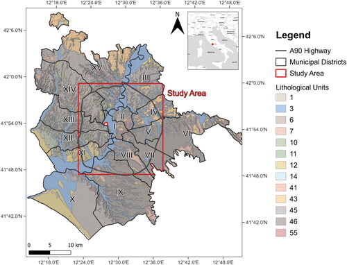
The area of interest (AOI) includes the Metropolitan City of Rome, extending from the historical centre to about the A90 highway (Figure 1). The city of Rome is situated in a hilly region characterized by a diverse geological and geomorphological setting. The geological formations consist of marine deposits (late Pliocene to lower Pleistocene), and continental sediments (middle Pleistocene – Holocene). These deposits, including marine clays, silt, silty sands, and transitional sediments, are prominently exposed on the hills along the right bank of the Tiber River. Additionally, volcanic deposits from the Colli Albani and Sabatini Volcanic Districts alternate with continental sediments, such as alluvial and palustrine deposits (middle to upper Pleistocene) (Figure 1).

Figure 1. Lithological units in the Municipality of Rome with the municipal districts, the study area, and the A90 highway outlined. Key to legend: 1: anthropic deposits; 3: recent and terraced sandy-gravelly alluvial deposits; 6: silty-sandy alluvial deposits, fluvio-lacustrine deposits; 7: travertines; 10: Plio-Pleistocene clayey and silty deposits; 11: marine Pliocene clays; 12: debris and talus slope deposits, conglomerates and cemented breccias; 14: marls, marly limestones and calcarenites; 41: leucitic/trachytic lavas; 43: lithoid tuffs, pomiceous ignimbritic and phreatomagmatic facies; 45: welded tuffs, tufites; 46: pozzolanic sequence; 55: alternance of loose and welded ignimbrites. EPSG:4326.

The present-day landscape is shaped by the Tiber River and its tributaries, which have carved valleys and slopes. The river valleys are partially filled with alluvial deposits, reaching considerable thicknesses (Bozzano et al. 2000). The groundwater circulation is controlled by the superimposition of permeable volcanic deposits over less permeable clayey and silty horizons, resulting in the development of ephemeral and perched water tables, such as those forming within the weathered soil covers and contributing to surface seepage in unsaturated soils. The different geological units on the left and right embankments of the Tiber River valley play a significant role in the response to natural and anthropogenic hazards affecting the urban area. Hazards such as subsidence, sinkholes, landslides, and floods have been previously experienced and assessed by several studies (Alessi et al. 2014; Bozzano et al. 2015a; Delgado Blasco et al. 2019; Esposito et al. 2021, 2023).

Landslides are often localized within unsaturated soil covers originated from Plio-Pleistocene sedimentary units. Intense and prolonged rainfall events have been identified as triggering factors for many slope failures, causing significant damage to infrastructure such as pipelines, aqueducts, and roads (Amanti et al. 2008; Alessi et al. 2014; Esposito et al. 2023).

Landslides and natural or anthropogenic sinkholes are the most common and impactful processes in the urban area. Sinkholes concentrate primarily in sectors characterized by the presence of volcanic deposits that were extensively exploited as a mineral resource since ancient Roman times. Consequently, a dense network of underground cavities exists, the majority of which remain undiscovered (Ciotoli et al. 2014, 2016; Esposito et al. 2021). According to Bianchi Fasani et al. (2011), these cavities experience an upward migration of the tunnel crown within the volcanic subsoil, eventually leading to the formation of sinkholes. Due to the predominantly brittle behaviour of cap rocks, particularly tuffs, abrupt failures following minimal deformations may occur, thus affecting effective monitoring for early-warning purposes (Esposito et al. 2021).

Numerous instances of land subsidence in Rome have been identified and quantified using multi-temporal InSAR techniques (Campolunghi et al. 2007; Cigna et al. 2014; Bozzano et al. 2015b; Delgado Blasco et al. 2019). The subsidence processes primarily occur in the alluvial sediments along the Tiber River and are mainly attributed to the load imposed by relatively recent urban development on the unconsolidated alluvial deposits. The subsidence rate in the region varies depending on the age of the constructed structures and the geological characteristics of the underlying formations (Bozzano et al. 2018; Delgado Blasco et al. 2019).

3. Materials and methods

In this work, multi-risk assessment is conceived as the process of assessing different independent hazards threatening individual buildings. We assume landslides, sinkholes, and subsidence as compound threats with no interrelationships between them (Kappes et al. 2012b; Tilloy et al. 2019; Hochrainer-Stigler et al. 2023).

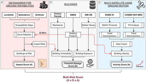
In this framework, a new workflow to identify and rank urban assets at risk (e.g. buildings) integrating hazard maps, multi-frequency PS-InSAR data and building features was developed. We underline that cultural heritage and religious structures were neglected in the present study due to the complexity of estimating their economic and vulnerability value. The workflow of the proposed methodology is reported in Figure 2. It consists of three main sections where geo-hazards probability for ground instabilities (a), building features (b), and multi-frequency InSAR displacement rates (c) are analysed and integrated to achieve both single- and multi-risk values. Each section results in a score that makes up the specific risk and subsequently the multi-risk ranking of analysed buildings.

Figure 2. Flowchart of the adopted methodology to compute buildings’ single- and multi-risk scores. Coloured subplots report the workflow to derive the hazard (a), potential damage (b) and activity (c) components of the multi-risk equation. In bold the main inputs and outputs data.

A detailed description of the implemented workflow and methods of achieving risk components is discussed in the following chapters. The entire data analysis process was automated via an implemented Python code freely available on the author’s GitHub page (https://github.com/gmastrantoni/mhr) together with the input data (Table 1).

Table 1. Input data with features and role in the multi-risk ranking. ISTAT (istituto nazionale di STATistica) stands for ‘national institute of statistics’.

Input data	Description	Risk component	Format	Website/reference
Landslide susceptibility map	Spatial probability of landslides occurrence	Hazard	Raster (5 × 5m)	Esposito et al. (2023) Mastrantoni et al. (2023)
Subsidence susceptibility map	Spatial probability of subsidence occurrence	Hazard	Raster (5 × 5m)	Research contract CERI – ACEA ‘Development of a monitoring and prevention plan of the geo-hydrological instability of the city of Rome’
Sinkhole susceptibility map	Spatial probability of sinkhole occurrence	Hazard	Raster (5 × 5m)	Esposito et al. (2021), and Research contract CERI – ACEA.
ISTAT census tracts	Spatial distribution of building features	Vulnerability	Vector (polygons)	https://www.istat.it/
DBSN database	Building footprints and features	Building type and footprint	Vector (polygons)	https://www.igmi.org/
OMI database	Asset market value	Exposure	Vector (polygons)	https://www.agenziaentrate.gov.it/portale/
Sentinel-1 PS time series	Spatial distribution of ground motion rate	Activity	Vector (points)	https://land.copernicus.eu/pan-european/european-ground-motion-service
Cosmo-SkyMed PS time series	Spatial distribution of ground motion rate	Activity	Vector (points)	https://www.asi.it/en/earth-science/cosmo-skymed/
DTM	Elevation	Topography	Raster (5 × 5m)	Esposito et al. (2023)
ReNDiS	Mitigation Measures	Validation	Vector (points)	http://www.rendis.isprambiente.it/rendisweb/

Note: DBSN (DataBase di Sintesi Nazionale) stands for ‘national synthesis database’. OMI (Osservatorio Mercato Immobiliare) stands for ‘real estate market observatory’. ReNDiS (repertorio Nazionale degli interventi per la difesa del suolo) stands for ‘national inventory of soil protection interventions.

3.1. Spatial multi-hazard assessment

This section describes the materials and methods applied for the assessment of multiple single hazard scores related to elements exposed to ground instabilities, as depicted in Figure 2(a).

3.1.1. Hazard score

In this work, we considered the spatial component of the hazard, which is the susceptibility, since the analysed ground instabilities are based on completely different processes with peculiar characteristics. Hence, the need to standardize the data to common information arises. Among the three geohazards considered in the present study, the temporal component of the hazard factor is conceptually definable for landslides only. Given the nature of subsidence, it occurs as a continuous (and non-linear) process that may be triggered by overloads and/or vary its intensity with time (e.g. velocity of settlements) up to the end of the process, thus preventing the assignment of return time values, as for landslides. A similar reasoning applies to sinkholes. A sinkhole can be interpreted as a unique shock event occurring in a confined place, which will no longer experience it. For this reason, sinkholes do not have a return time, nor have significant relationship with recurrent triggers pointed out so far. Given that, we decide to use high-resolution susceptibility maps as the hazard component of risk. Susceptibility maps report the spatial probability of occurrence of a certain event without considering the temporal dimension. They represent one of the products that lead to a comprehensive hazard assessment (Cascini 2008; Fell et al. 2008; Corominas et al. 2013). According to Corominas et al. (2013), susceptibility assessment can be considered an end product that can be used in land-use planning and environmental impact assessment. As demonstrated by Mastrantoni et al. (2023), a measurable loss in accuracy, and thus in reliability for specific purposes (Cascini 2008), is proportional to the decrease in zoning scale.

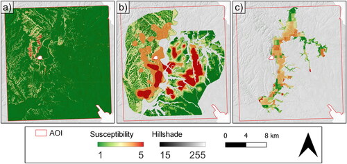
Susceptibility maps are represented in raster format with a resolution of 5 metres and cover the entire centre of Rome (Figure 3). Each raster cell gives the level of probability of being affected by a landslide (Figure 3(a)), a sinkhole (Figure 3(b)), and a subsidence (Figure 3(c)). The value of susceptibility ranges from 1 to 5, where 1 stands for negligible and 5 for very high probability. The employed landslide and sinkhole susceptibility maps derive from already published studies (Esposito et al. 2021, 2023; Mastrantoni et al. 2023). Susceptibility to subsidence was commissioned to Sapienza University of Rome by ACEA ATO2 Spa that funded a project for a better knowledge of hazards aimed at safeguarding the underground service network in Rome.

Figure 3. Susceptibility map for landslides (a), sinkholes (b) and subsidence (c) within the area of interest (AOI).

The landslide susceptibility map was obtained by applying the extra trees classifier (Pedregosa et al. 2011), a supervised machine learning model that has proved to outperform several other algorithms (Mastrantoni et al. 2023). The model was trained and tested with a database of about 3000 landslide initiation and stable points distributed throughout the Municipality of Rome.

The sinkhole susceptibility map refers to anthropogenic sinkholes of Rome mainly due to the presence of underground cavity networks in areas featured by relevant thickness of volcanic deposits (Bianchi Fasani et al. 2011) and to ‘piping-like’ processes due to shallow groundwater circulation and related erosion of silty fraction of layers in area dominated by sedimentary sequences. The assessment was carried out through the logistic regression multivariate statistical technique taking advantage of a database containing about 1000 sinkholes that occurred in the period 1875–2018.

Lastly, the subsidence susceptibility map was realized by reconstructing the extent and thickness of recent alluvial deposits. This process was based on the interpolation of available stratigraphic logs throughout the valley of the Tiber River. The derived thickness map of recent alluvial deposits was then weighted based on their type, thickness, and depth within the stratigraphic sequence, considered as proxies of compressibility, and thus proneness to develop consolidation settlements.

To derive the multiple single-hazard scores, the built environment was analysed with the zonal statistics method, thus retrieving the maximum value of hazard class within the perimeter of individual buildings. Elements with a hazard score above 2 were considered exposed to a specific single risk. We stress that to account for landslide run-outs, a buffer of 20 m was drawn around the buildings. The buffer size was calibrated on the mapped landslides within the territory of Rome, as reported by Alessi et al. (2014) and Del Monte et al. (2016).

3.1.2. Impact ratio

Since susceptibility maps do not directly provide magnitude information in terms of dimension and volume of the process, a strategy to overcome this limitation and define a proxy for hazard intensities was needed. Consequently, it was assumed that the potential magnitude of the hazards impacting the built environment is directly related to the percentage of the building’s area exposed to the threat. To achieve this information, building footprints were overlaid on susceptibility maps and a categorical zonal statistic was computed, thus counting, and weighting the hazard classes within the polygons. By setting the threshold for the hazard class equal to 2 (i.e. low susceptibility) the weighted area of the element exposed to risk was derived, and consequently the ratio of the total area. Such information, hereafter called impact ratio (I_b), is then coupled in the following phases with structural resistance for the assignment of physical vulnerability values to the specific ground instability hazard. The values of the impact ratio were classified into four classes using equal intervals. I₀ is defined by an impact ratio equal to 0, I₁ for 0 < I_b≤0.25; I₂ for 0.25 < I_b≤0.5; I₃ for 0.5 < I_b≤0.75 and I₄ for I_b>0.75. Therefore, each element within the area of interest has one or more impact ratio classes following the threats to which it is exposed.

3.2. Multi-hazard consequence analysis

This section describes the materials and methods applied for quantifying the potential multi-hazard damage scores of the built environment, as depicted in Figure 2(b).

3.2.1. Vulnerability

Building vulnerability was defined according to the impact ratio of the i-th hazard and the structural resistance of buildings. The definition of structural resistance relies on the approach proposed by Li et al. (2010) for landslide hazards and modified by Caleca et al. (2022). In this study, we assume that structural resistance to landslides can also be considered valid for sinkhole and subsidence hazards.

The applied approach exploits census tract data produced by ISTAT in 2011 (Table 1) and impact ratio data. It consists of three phases. First, the estimation of the structural resistance for each census tract within the area of interest was made by using a modified equation proposed by Li et al. (2010) and Caleca et al. (2022): (1) $$R_{\mathit{str}}={\left({\epsilon }_{\mathit{sty}}\times {\epsilon }_{\mathit{smn}}\times {\epsilon }_{\mathit{sht}}\right)}^{1/3}$$(1) where ${\epsilon }_{\mathit{sty}},$ ${\epsilon }_{\mathit{smn}},$ and ${\epsilon }_{\mathit{sht}}$ are resistance factors of structure type, maintenance state and number of floors, respectively. These parameters are derived from census tract data (Table 2). The Italian census tracts are delineated as geographically contiguous areas within the country’s territory that demonstrate a notable degree of homogeneity. Each census tract represents either an entire municipality, a specific portion thereof, or a cluster of municipalities characterized by comparable environmental and socioeconomic features. They provide comprehensive information pertaining to the characteristics of buildings within the area, encompassing factors such as typology, quantity, materials, and other relevant attributes. Furthermore, census tracts offer valuable insights into population distribution. Values of resistance factors are set according to that suggested by previous studies (Li et al. 2010; Caleca et al. 2022) (Table 2), and combined with impact ratio values to retrieve the vulnerability level.

Table 2. Values of resistance factors employed in the structural resistance assessment (from Caleca et al. 2022).

Resistance factor	Parameter	Typology	Value
Structure type	ɛsty	Productive and commercial	0.1
		Residential with light structure	0.2
		Residential with brick walls	0.8
		Residential reinforced concrete	1.5
Maintenance state	ɛsmn	Productive and commercial	0.1
		Residential in very poor condition	0.1
		Residential in a medium condition	0.6
		Residential in a good condition	1.2
		Residential in a very good condition	1.5
Number of floors	ɛsht	Productive and commercial	0.1
		Single-storey residential	0.1
		Two-storey residential	0.4
		Three-storey residential	0.9
		Number of floors ≥4	1.5

The second step of the procedure consists of the attribution of the structural resistance values (R_str) computed from the census tracts to the corresponding building depending on its position and type (i.e. residential/not residential). Following that, a classification was conducted, categorizing the built environment into six distinct classes based on their respective level of structural resistance (Table 3). Footprints and categories of use of the built environment were extracted from the DBSN database (Database di Sintesi Nazionale) (Table 1). It is freely available under the Open Data Commons Open Database Licence (ODbL). The DBSN database is a geographic database containing territorial information primarily derived from regional geo-topographic data. These data have been harmonized and standardized within the structure to ensure national homogeneity while preserving the original level of detail. Administrative boundaries are derived from cadastral data, ensuring congruence with municipal and state administrative borders. The built environment is classified into detailed categories of use.

Table 3. Contingency matrix for the assessment of building vulnerability by means of impact ratio and structural resistance classes (modified from Caleca et al. 2022).

Resistance	Impact ratio
	I0	I1	I2	I3	I4
R4	0	0	0.25	0.25	0.50
R3	0	0.25	0.25	0.50	0.50
R2	0	0.25	0.50	0.50	0.75
R1	0	0.25	0.50	0.75	0.75
R0	0	0.25	0.75	0.75	1
N.A.	0	0	0	0	0

The third phase of the applied approach involved the quantification of the multi-hazard vulnerability values for each element at risk. These values were obtained using the contingency matrix proposed by Caleca et al. (2022) and tailored to this study, to established a link between the classes of the impact ratio for the i-th hazard type and the classes of structural resistance (Table 3). The contingency matrix defines five distinct vulnerability classes: V₀ (null vulnerability), V₁ (low vulnerability), V₂ (medium vulnerability), V₃ (high vulnerability), and V₄ (very high vulnerability). To calculate quantitative values for vulnerability, which were necessary for assessing the economic potential damage, numerical values ranging from 0 to 1 were assigned to each vulnerability class as follows: V₀ = 0, V₁ = 0.25, V₂ = 0.5, V₃ = 0.75, V₄ = 1. Hence, each building has been assigned one or more vulnerability values depending on the number and type of hazards to which it is exposed.

3.2.2. Exposure

In this study, exposure of elements at risk (E_b) is deemed as the economic value per square metre, taking the real estate’s market value as a reference. To obtain this information, we exploited the OMI national-scale open access database (which stands for Osservatorio Mercato Immobiliare – real estate market observatory) (Table 1). It is managed and updated every six months by the National Revenue Agency under the Italian Ministry of Economy and Finance. The OMI dataset encompasses comprehensive information regarding the minimum and maximum market values for various building typologies, expressed in euros per square metre (€/m²). These data are aggregated at the municipality level and further stratified into smaller subdivisions, known as ‘OMI zones’, within the respective municipality. The study area includes 186 zones. Market data related to the first semester of 2022 were downloaded and pre-processed to define for each OMI zone the average market value of six peculiar building typologies: economic, retail, residential, office, and industrial (Figure A1 in Appendix A). Thereafter, categories of use from the DBSN database were linked to typologies from OMI zones, and the respective economic values were associated according to location and type of buildings.

3.2.3. Potential damage score

To quantify the potential damage, multi-hazard vulnerabilities were combined with the previously derived exposure values (Marzocchi et al. 2012), thus obtaining the expected economic loss per square metre (LOSS_b): (2) $${\mathit{LOSS}}_b\left(h\right)=V_b\left(h\right)\times E_b$$(2) where V_b(h) is the vulnerability value of building exposed to the hazard h, and E_b represents its economic value expressed in euros per square metre.

Once the potential multi-hazard loss data were derived, the empirical cumulative distribution function (eCDF) was applied to them. With this approach, we sorted and ranked the damage data without making assumptions about the underlying probability distribution. The eCDF quantifies the proportion of data points that are less or equal to a given value. By exploiting the cumulative distribution of potential economic losses, class thresholds were set following Equation (3)(3) $$D_b\left(h\right)={\mathit{eCDF}}^{-1}\left(p,\mathrm{ }\mathit{LOSS}\left(b|h\right)\right),\mathrm{ }p=(20,40,60,80)$$(3) and potential damage scores (D_b) ranging from 1 to 5 were defined. (3) $$D_b\left(h\right)={\mathit{eCDF}}^{-1}\left(p,\mathrm{ }\mathit{LOSS}\left(b|h\right)\right),\mathrm{ }p=(20,40,60,80)$$(3) where ${\mathit{eCDF}}^{-1}$ denotes the inverse of the empirical cumulative distribution function, $p$ is the specific value of the proportion or percentile for which the damage score D_b was calculated. $\mathit{LOSS}\left(b\right|h)$ represents the distribution of economic loss values of buildings ($b$) considering only those exposed to the hazard $h.$ These class thresholds assist in delineating the severity levels of the potential economic loss associated with multiple hazards. We acknowledge that the ranking will be sensitive to the threshold values chosen to delimit the classes. However, the strength of it lies in being able to customize and optimize class thresholds according to the proportion of items to be contained in each class.

3.3. Multi-satellite SAR interferometry

This section describes the materials and methods applied for assessing the multi-hazard activity scores of the built environment, as depicted in Figure 2(c).

3.3.1. Interferometric analysis

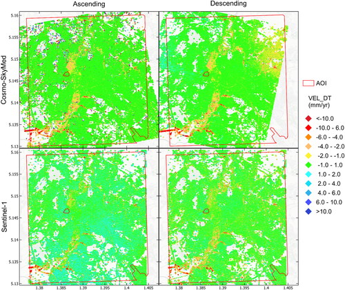
In this study, the Advanced-DInSAR (A-DInSAR) technique (Hanssen 2001) was employed to derive displacement rates throughout the area of interest. The A-DInSAR method is increasingly applied to study the temporal evolution (by means of time series) of ground displacements for objects with long-term stability in terms of reflectivity, known as Persistent Scatterers (PS) (Ferretti et al. 2001). The PS-InSAR technique extracts this information from a huge collection of SAR images, forming an interferometric stack that enables the derivation of displacement patterns over the desired time span. The dataset accessed in this study was acquired from two currently active satellite SAR missions that provide freely available historical archive data for scientific research: Sentinel-1 (by ESA) and Cosmo-SkyMed (by ASI). The main differences between these images lie in the resolution, both temporal and geometrical, and in the acquisition bandwidth (C- and X-band respectively). Sentinel-1 (S1) has a pixel resolution of 5 × 20 m on the ground, while Cosmo-SkyMed (CSK) has a resolution of 3 × 3 m (for the Interferometric Wide images used and available from the archive). The revisit time of the S1 constellation is higher than CSK. The former being approximately 6 days (until 23 December 2021, end date of the Sentinel-1B mission), whereas the latter being 16 days on average. This is due to its dual-purpose mission for both civilian and military applications. Moreover, it may have sparse missing data.

The S1 PS derive from the European Ground Motion Service products (EGMS). The EGMS is part of the Copernicus Land Monitoring Service and applies the PS-InSAR technology to monitor ground deformations over most of Europe (Costantini et al. 2021). The data employed in this study refers to Level 2a, which is the first of three product levels (Costantini et al. 2021; Crosetto et al. 2021). This level is also called Basic Product, it includes displacement rates and time series measured along the Line of Sight (LOS) for both the ascending and descending orbital geometries. According to Crosetto et al. (2021), these data are suitable to study local deformation phenomena such as subsidence, landslides, tectonic effects, and earthquakes, which impact the stability of slopes, buildings and infrastructures. The resultant PS time series data covers a period of seven years (from 10 February 2015 to 23 December 2021), with a temporal sampling of one image every six days.

The CSK dataset, not yet available from the EGMS project, was elaborated using the PS approach starting from a total of 358 SAR images retrieved from the archives of the Italian Space Agency (ASI), which provides free of charge data for academic purposes. The selected time span ranges from 2010 to 2022 for both orbital geometries:

• Ascending orbital geometry: 196 images in Single Look Complex (SLC) format acquired by the CSK satellites from 04 July 2010 to 19 July 2022.

• Descending orbital geometry: 162 images in Single Look Complex (SLC) format acquired by the CSK satellites from 27 July 2010 to 19 June 2022.

For each geometry in each dataset, a master image was selected as the reference for the calculation of phase differences in other images within the dataset. The master image for the descending dataset was captured on 17 December 2017, and for the ascending dataset on 28 May 2014. The displacement rate values (here expressed in mm/year) estimated by the A-DInSAR analysis for all the PS are relative to the selected reference point. The reference point for the ascending dataset was located at LAT = 41.8868, LON = 12.4914 and for the descending dataset at LAT = 41.8879, LON = 12.4405 (EPSG:4326). Finally, the analyses were calibrated and validated with displacement data acquired from GNSS stations (Ferretti et al. 2022). The greater ground resolution of the CSK SAR images provided a denser PS coverage than the S1 products. Indeed, the total number of PS within the area of interest is about 4.65 × 10⁶ and 1.46 × 10⁶ for CSK and S1 descending geometry respectively.

Displacement time series can be divided into three parts that include seasonal, trend, and remainder components. The latter containing random fluctuations and noise (Costantini et al. 2018; Hyndman and Athanasopoulos 2018). Hence, the need to decompose PS time series to extract the long-term trend arises. To this purpose, we applied a Seasonal-Trend Decomposition (STL) technique (Cleveland et al. 1990) based on a LOcally wEighted regreSsion Smoother (LOESS) (Figure 4), which is implemented within the PS-ToolBox plugin for QGIS developed by Nhazca (https://www.sarinterferometry.com/ps-toolbox/).

Figure 4. PSs map of average velocity along LOS computed from long-term trends extracted from Sentinel-1 and Cosmo-SkyMed for ascending and descending orbits. EPSG:3857.

3.3.2. Data fusion

S1 and CSK PS time series were then merged for cross-validation and to gain reliability, as well as to increase spatial coverage of displacement information. The implemented data fusion method within the PS-ToolBox allows the integration of multi-mission PS data. The combination of multiple sources measurements, with different orbital geometries, exploits the strain tensor (Guglielmino et al. 2011) through the ESISTEM (Extended Simultaneous and Integrated Strain Tensor Estimation from Geodetic and Satellite Deformation Measurements) (Luo and Chen 2016) method to generate synthetic datasets that incorporate multi-band information. The estimated displacement ($D_{\mathit{LOS}}^k\left(\mathrm{X}\right), k=1,\dots , K$) of each synthetic data point ($\mathrm{X}=(x,y)$) along the k LOS is determined by combining the ground deformation components (i.e. the vertical Up-Down and horizontal East-West displacement, $f_i\left(X\right), i=(1,2)$) and the direction cosine ${(S}_i^k,\mathrm{ }\mathrm{i}=(1,2)$) of the k LOS: (4) $$D_{\mathit{LOS}}^k\left(X\right)=S_1^k{f}_1\left(X\right)+S_2^k\mathrm{ }{f}_2\left(X\right),\mathrm{ }k=1,\mathrm{ }\dots ,\mathrm{ }K$$(4)

The deformation components are estimated using the known N neighbour PS points ($X_n=(x_n,y_n$), n = 1, …, N) along each k LOS through the formulation of a first order Taylor polynomial: (5) $$D_{\mathit{LOS}}^k\left(X_n\right)=D_{\mathit{LOS}}^k\left(X\right)+\nabla D_{\mathit{LOS}}^k\left(X\right)\Delta X_n$$(5) where $\Delta X_n$ contains the relative distances between the $X_n$ point components and the synthetic point $X.$ The displacement map along the multi-satellite LOS is found by solving the Taylor system for the K LOS. The data fusion formulation considers two parameters: the maximum distance within which nearby PS measurements are selected to estimate deformations, and the locality factor that weights the contribution of each measurement based on its distance from the point estimation. The synthetic datasets of Up-Down and East-West components are derived into a regular grid of squared cells from the vector decomposition of the displacement map along the multi-satellite LOS.

3.3.3. Activity score

The vertical and horizontal components of ground displacement achieved by the fusion of S1 and CSK PS data were further processed with building footprints. Points contained within each polygon were interpolated to produce a raster with mean velocity values over the time span at 10 metres grid resolution. This procedure results in a series of velocity values for each element within the area of interest. With the aim of quantifying the state of activity of each element in reference to the hazard to which it is exposed, three specific values of velocity were retrieved from individual building statistics and assigned to the whole element at risk. For the landslide hazard, the maximum absolute velocity between the vertical and horizontal components was selected. Regarding the subsidence hazard, we computed the range between minimum and maximum vertical velocity, thus focusing on buildings experiencing distortion; and concerning the sinkhole hazard, the maximum negative velocity of the vertical component was preferred.

Once the specific hazard velocities were assigned to the entire built environment, we applied the same approach employed to rank potential damage. Therefore, Equation (6)(6) $$A_b\left(h\right)={\mathit{eCDF}}^{-1}\left(p,\mathrm{ }\mathit{VEL}\left(b\right|h)\right),\mathrm{ }p=(50,\mathrm{ }82,\mathrm{ }95,\mathrm{ }97.5)$$(6) was applied to derive class thresholds of the building velocity. According to the eCDF in Equation (6)(6) $$A_b\left(h\right)={\mathit{eCDF}}^{-1}\left(p,\mathrm{ }\mathit{VEL}\left(b\right|h)\right),\mathrm{ }p=(50,\mathrm{ }82,\mathrm{ }95,\mathrm{ }97.5)$$(6) , class thresholds were set at the respective percentile ($p$) value, and activity scores ($A_b$) ranging from 1 to 5 were defined. (6) $$A_b\left(h\right)={\mathit{eCDF}}^{-1}\left(p,\mathrm{ }\mathit{VEL}\left(b\right|h)\right),\mathrm{ }p=(50,\mathrm{ }82,\mathrm{ }95,\mathrm{ }97.5)$$(6)

3.4. Multi-risk ranking

To derive multi-risk scores, we firstly ranked the specific risk of single hazards by combining the three risk components described above. Equation (7)(7) $$R_b=H_b\left(h\right)\times A_b\left(h\right)\times D_b\left(h\right)$$(7) defines the convolution of the hazard ($H_b(h)$), activity ($A_b(h)$), and potential damage ($D_b(h)$) that compose the single-risk score ($R$) of each exposed building ($b$). (7) $$R_b=H_b\left(h\right)\times A_b\left(h\right)\times D_b\left(h\right)$$(7)

Secondly, starting from the single-risk evaluations ($R_b$), the multi-risk score at building level (${MR}_b$) is defined as their summation corrected by a multiplication factor ($F_h$) (Equation (8)(8) $${MR}_b=\sum _{\mathit{All}\mathrm{ }\mathit{risks}}(R_b\times F_h)$$(8) ). This coefficient weights the risk score by the corresponding hazard type, depending on whether it is a shock or a stress process. This is because stress phenomena usually cause fewer losses than shock ones and are also harder to mitigate. Regarding shock events such as landslides and sinkholes, the $F_h$ coefficient is set equal to 1, thus keeping the risk score unchanged. Whereas, in the case of stress processes (e.g. subsidence) we decided to fix the $F_h$ coefficient equal to 0.5. (8) $${MR}_b=\sum _{\mathit{All}\mathrm{ }\mathit{risks}}(R_b\times F_h)$$(8)

Finally, a spatial distribution of dominant risk among the built environment was retrieved by selecting the maximum value across single risk scores and assigning the corresponding hazard to it.

Once obtained, both the single- and multi-risk scores were rescaled to five classes using the eCDF based method and percentiles described above, thus clustering assets with risk level in the top 2.5%, 5%, 18%, 50%, and lower than median into scores ranging from 5 to 1, respectively.

Finally, to validate the results, financial data related to expenses incurred for remediation and mitigation measures within the AOI were retrieved from the ReNDiS database (Table 1) and compared with the multi-risk scores of nearby buildings.

4. Results

4.1. Hazard

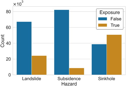
The exposure analysis to ground instabilities of urban assets within the area of interest assigned a binary classification (i.e. exposed/not exposed) to each individual building. As a result, the threat to which most buildings are exposed proves to be the sinkhole hazard (Figure 5), as more than half of the elements were found to be at risk. Additionally, about 10% of the built-up area might be affected by subsidence processes, while landslides pose a potential risk to about one-third of the buildings.

Figure 5. Overall number of buildings exposed (true) and unexposed (false) for each type of hazard investigated.

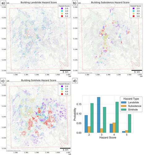
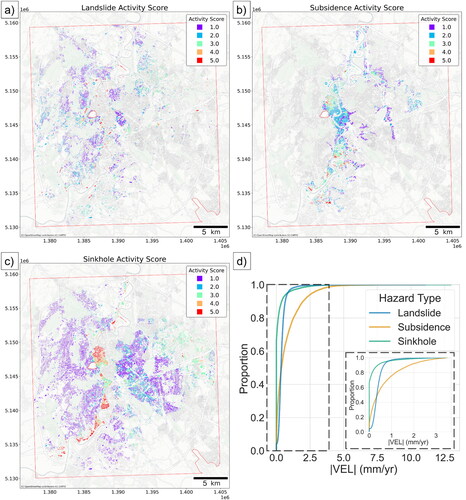
Further investigation into the specific elements exposed to each threat revealed their hazard score, which was subsequently mapped (Figure 6). Figure 6(d) reports the statistical distribution of the elements at risk across assigned hazard scores. Landslide-prone buildings are mainly ranked with a hazard score of 3, with just a few having the maximum hazard. Spatially, they spread throughout the northwestern and southern slopes (Figure 6(a)). The sinkhole hazard score seems to distribute almost equally, and the same applies to subsidence hazard. However, subsidence hazard spread along the valleys and paleo-valleys of the Tiber and Aniene Rivers (Figure 6(b)), whereas the highest sinkhole hazard scores concentrate among the S-E part of the city (Figure 6(c)).

Figure 6. Hazard score of buildings for landslides (a), subsidence (b), and sinkholes (c). Statistical distribution of hazard score for elements at risk by hazard type (d). EPSG:3857.

4.2. Potential damage

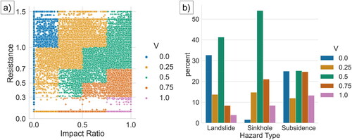
Figure 7(a) illustrates the probability density function (PDF) of impact ratio values by different ground instability types. The distributions of impact ratios exhibit similarities between landslide and subsidence, with values spread over the range. A slight deviation towards higher values is observed for subsidence. Conversely, the impact ratio values for sinkholes tend to concentrate around 0.8.

Figure 7. Probability density functions of impact ratio values by hazard type (a), and of structural resistance values for residential buildings.

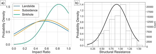
Structural resistance values were obtained for both residential and non-residential buildings (i.e. productive, and commercial). In Table 2, the reported parameters reveal that resistance values for non-residential constructions consistently equate to 0.1, as no structural characteristics are included in the census tract data. Contrarily, for residential buildings, the resistance values can vary between 0 and 1.5. Figure 7(b) displays the histograms along with the PDF of computed structural resistance values specifically for residential buildings, which have a mean value of 0.9 and a standard deviation of 0.28.

Once reclassified, impact ratio and structural resistance were merged to form vulnerability classes using the contingency matrix presented in Table 3. The pairs of impact ratio and resistance values are illustrated in Figure 8(a), with distinct colours indicating the assigned vulnerability value. This graphical representation effectively shows the boundaries of the vulnerability classes. The resultant multi-hazard physical vulnerability values (Figure 8(b)) exhibit a tendency to concentrate at 0 and 0.5 for landslides, with about 75% of the structures within the two classes. In the case of sinkhole events, about 55% of the buildings demonstrate a vulnerability value of 0.5 and 20% of 0.75. However, vulnerability to subsidence appears to be evenly distributed among values of 0, 0.5, and 0.75 for 80% of the buildings. Furthermore, it should be noted that among the others, subsidence hazard has the highest percentage of elements with vulnerability of 0.75 and 1.0, about 25% and 10% respectively.

Figure 8. Graphical representation of the vulnerability value (V) assignment based on the contingency matrix reported in Table 3 (a). Distribution of vulnerability value of elements at risk by hazard type (b).

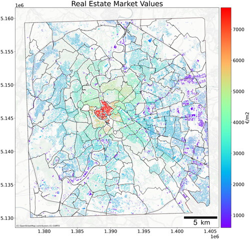
The analysis of real estate market data enabled the determination of economic value per square metre for each urban asset. Figure 9 presents the exposure of the built environment in the designated area of interest. Notably, there is a distinctive radial distribution pattern observed, with the highest values concentrated within the historic centre. These peak values exceed 7000 euro/m² and gradually decrease as one moves towards the suburbs. In suburban areas, the exposed value can be as low as 1000 euro/m². This applies particularly to the eastern sector, where a significant number of industrial activities are located.

Figure 9. Real estate market values of buildings per square metre (€/m²) within the study area according to their category of use and position. EPSG:3857.

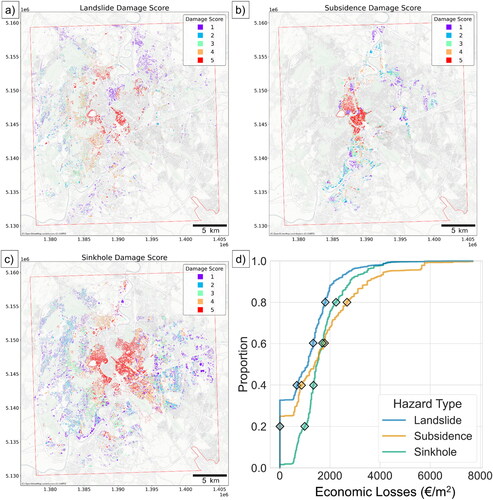
The integration of multi-hazard vulnerability and exposure values enabled the computation of potential economic losses per square metre. Subsequently, these losses were reclassified into potential damage scores, as depicted in Figure 10. Each element at risk was assigned a damage score based on the specific threats it is exposed to. The mapped damage scores for landslide, subsidence, and sinkhole can be observed in Figure 10(a–c), respectively. Furthermore, Figure 10(d) presents the eCDF of resultant potential economic losses. These eCDF were utilized to identify the score class thresholds, which are indicated by markers along the curves.

Figure 10. Potential damage score of buildings for landslides (a), subsidence (b), and sinkholes (c). Empirical cumulative distribution of economic losses per square metre selected according to hazard type (d). The coloured diamonds define percentile thresholds used to derive the five score classes. EPSG:3857.

4.3. State of activity

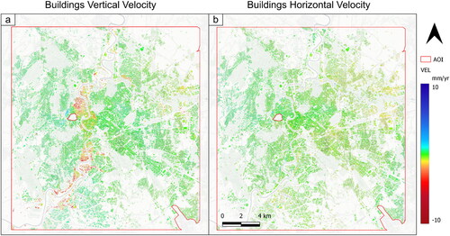
The synthetic datasets of vertical and horizontal components derived from the data fusion process of S1, and CSK PS time series are reported in Figure A2 (see Appendix A). The resulting displacement rates of the built environment are reported in Figure 11. A comparison between the two components reveals that displacements predominantly occur along the vertical axis (Figure 11(a)). The horizontal displacements exhibit minimal rates, peaking at a few mm per year (Figure 11(b)). Notably, the largest rates can be observed for assets situated along the Tiber River valley.

Figure 11. Buildings’ vertical (a) and horizontal (b) displacement rates (i.e. velocity) derived from the grid-based synthetic datasets (Figure A2) and assigned to the entire built-environment under investigation. EPSG:4326.

Based on the hazard-specific value distribution, activity scores were assigned to the building displacement rates. Figure 12(a–c) depict the resulting activity scores for landslide, subsidence, and sinkhole, respectively. Figure 12(d) presents the eCDF of the quantitative absolute velocity values, which were assigned to individual assets based on the hazard under consideration.

Figure 12. Activity score of buildings for landslides (a), subsidence (b), and sinkholes (c). Empirical cumulative distribution of absolute velocities values selected according to hazard type (d) employed to set up class thresholds. EPSG:3857.

4.4. Multi-risk

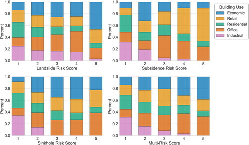
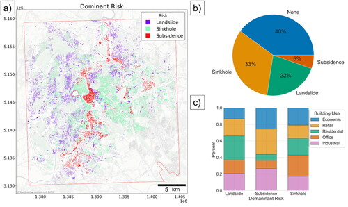
The rankings of landslide, subsidence, and sinkhole risks for individual buildings, derived from the combination of the corresponding hazard, damage, and activity scores, are illustrated in Figure 13(a–c), respectively. Moreover, the aggregation of single-risk scores using the appropriate weighting factor produced a multi-risk map, as shown in Figure 13(d). Examining the building use categories alongside their associated risk scores reveals that retail and economic structures exhibit the highest proportion of buildings with elevated risk scores, closely followed by offices (Figure A3 in Appendix A). In the case of residential buildings, they are distributed relatively evenly across the risk classes, although there is a slightly higher concentration within risk score 1. The dominant risk type of each element at risk is depicted in Figure 14(a). Out of the approximately 90 × 10³ urban assets analysed, it was determined that 60% of them are at risk. Within this group, 33% exhibit the highest risk score attributed to sinkhole phenomena, while 22% and 5% possess the highest score related to landslides and subsidence processes, respectively (Figure 14(b)). Delving into buildings’ use categories, it results that the dominant risk type is not evenly distributed among them, thus landslide risk prevails for residential buildings, while subsidence and sinkhole risks predominate for retail and offices, respectively (Figure 14(c)).

Figure 13. Risk score of buildings for landslides (a), subsidence (b), sinkholes (c) and multi-hazard (d).

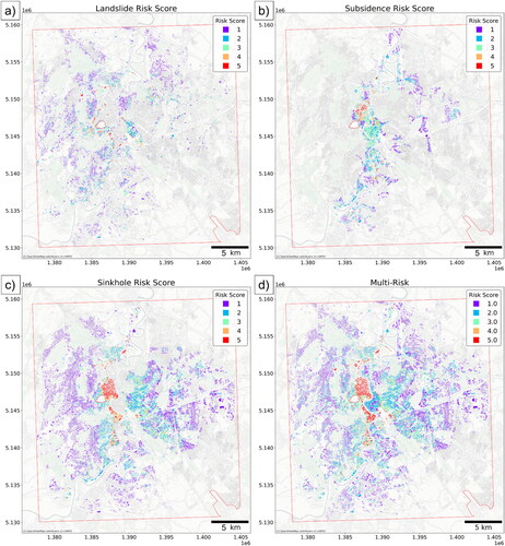
Figure 14. Spatial distribution of dominant risk threatening individual buildings (a) with a focus on the hazard type ratio among the overall elements (b), and among the buildings use categories (c).

5. Discussion

Risk assessment of natural hazards can guide preventive and corrective actions to reduce levels of vulnerability and hazard exposure of urban assets and populations.

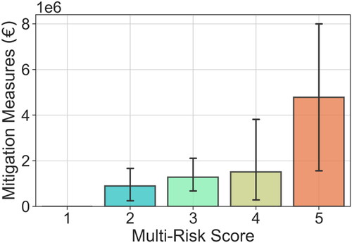
In this study, a semiquantitative multi-risk assessment was developed to provide a replicable and customizable framework for ranking and prioritizing elements at risk based on official open-source data. The approach relies on three factors (i.e. hazard, potential damage, and state of activity) that are combined to compute the specific- and multi-risk score of urban buildings. Albeit both temporal and spatial information should be considered to perform a proper hazard assessment (Fell et al. 2008), data on the recurrence and magnitude of ground instabilities in Rome are lacking, except for landslides (Esposito et al. 2023). The investigated ground instabilities rely on completely different geological processes that affect the possibility of estimating return periods. Moreover, they don’t seem to be triggered by any environmental variables. Hence, the hazard related score factors are only based on the spatial component (i.e. susceptibility) which was engineered to derive (i) the probability of individual elements being involved in an event in the near future (hazard score), and (ii) the building’s area potentially affected and weighted by susceptibility levels, as a proxy for the expected magnitude, and thus for the destructiveness of the event (impact ratio). The potential damage score is built upon building’s physical vulnerability and its economic value, which provide valuable results to quantify the potential economic losses. With respect to others (Papathoma-Köhle et al. 2007; Kappes et al. 2012a; Romão et al. 2016; Bianchini et al. 2017; Huang S et al. 2023) deriving the physical vulnerability from structural resistance values and hazard intensity facilitated the computation at large scale, since it exploits features of the built environment based on open-source official census tracts of Italy. Moreover, structural resistance parameters can be easily modified to suit specific hazards. The last risk component, i.e. activity score, provides a dynamic layer that relies on displacement rates of the elements within hazardous area. It employs the distribution of building velocity values retrieved from multi-satellite PS time series. The activity score is based on the fusion of S1 and CSK PSs, thus exploiting the strengths and overcoming the weaknesses of each dataset. According to Costantini et al. (2017), PS density from CSK images (X-band) is higher by one order of magnitude respect to C-band SAR (e.g. S1), especially for surfaces with reduced radar backscattering coefficient and without strong point-like scatterers, thus helping to better detect ground deformation phenomena affecting small areas (Esposito et al. 2021; Festa et al. 2022). Moreover, CSK sensor has higher sensitivity in detecting small movements. Conversely, S1 has significantly higher frequency and regularity, thus increasing the applicability for early detection of failure precursors. Hence, the fusion of PSs retrieved from both satellites ensured higher resolution and spatial coverage to catch ground instability processes in detail. Both potential damage and activity scores derive from the exploitation of the empirical cumulative distribution function, which allows the selection of threshold values equal to the specified fraction of observations (e.g. percentile). According to Mastrantoni et al. (2023), percentiles must be chosen based on values distribution and expert judgment. Therefore, class thresholds can be easily adapted to other cities. For the city of Rome, the top 2.5% of buildings at multi-risk were selected as the highest class. However, the number of elements in the highest priority class may be set depending on the availability of funds for mitigation measures. The ReNDiS database states a total amount of expenses financed for mitigation measures within the area of interest of approximately 97 million euros, encompassing 71 projects. These data enable us to compare and validate the multi-risk outcomes using official financial records (Figure 15). The average cost of mitigation rises progressively as the multi-risk class of the nearby buildings increases, thus revealing a significant correlation between mitigation expenses and calculated multi-risk score that ensure the reliability of the proposed method.

Figure 15. Average expenses (M€) and standard deviations of incurred mitigation measures within the study area compared with the multi-risk score of nearby buildings as computed in this work.

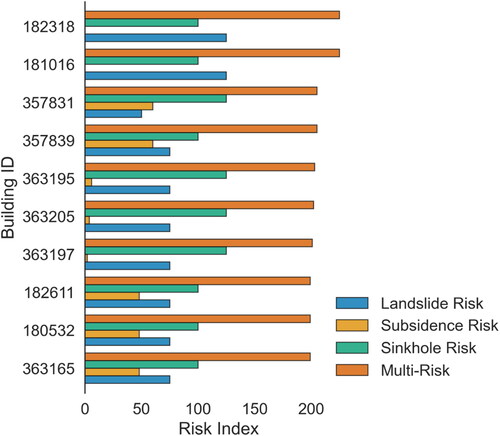
Multi-risk scores can also be analysed prior to reclassification, thus retrieving the buildings with the absolute highest indices (Figure 16). As expected, the most at-risk buildings may face all three ground instabilities investigated, although landslide and sinkhole risk generally overwhelm subsidence risk. This is mainly related to the F_h coefficient halving the risk of subsidence, since stress phenomena, such as subsidence, are hereby considered less urgent and impactful in terms of mitigation measures and expected economic losses respectively.

Figure 16. Ranking of the top 10 buildings with the highest absolute risk within the study area.

The developed model is intended as an alternative to other risk assessment approaches requiring very demanding tasks, such as quantitative probabilistic hazard scenarios and fragility curves. The workflow is completely automated and customizable. More hazards related to ground deformations can be easily added, albeit not considering potential interrelationships. Structural resistance parameters can be adapted to suit the hazard characteristics and percentile thresholds defining the scores can be modified to fit stakeholders needs. The data availability at national scale unlocks its replicability throughout Italy, thus enhancing the scalability of the approach. Moreover, by exploiting individual urban assets and their features allowed us to perform the analyses at the real scale (i.e. 1:1). Further advantages of the multi-risk ranking approach presented in this study are (i) its complete objectivity in conducting the analyses without any assumption on the input data, (ii) its site-specific risk prioritization of structures for natural hazards mitigation, and (iii) the possibility of updating the results using up-to-date satellite InSAR monitoring data. However, it has some limitations. Hazards interactions, and therefore amplified vulnerability and risk, are not evaluated due to the challenges of performing multi-hazard scenarios modelling for ground instabilities. The hazard component of the risk equation is derived from spatial probability without considering the temporal factor, thus static risk and multi-risk scores are defined. Although the application in the selected case study did not account for structural resistance parameters variations depending on hazard type, the optimization of such parameters based on historical data and expert judgement may improve the quality of results. Thus, future research and development will focus on the integration of additional geohazards, such as earthquakes and floods, and the optimization of building data, with the aim of also assessing cultural heritage, currently omitted due to the lack of official data on economic value and vulnerability. A huge effort will also be devoted to multi-hazard scenario modelling aimed at correlating the three components of the hazard (i.e. space, time, and intensity) and evaluating potential hazard interactions, which will unlock a quantitative multi-risk assessment. A key point is represented by the expected costs of mitigation actions. Their estimation will have a significant impact on stakeholders involved in risk management for large cities. Nowadays, ever more accurate data is being collected and released through databases often with open access. The new census tracts of Italy from ISTAT will contain data about hospitals, schools and other non-residential structures that may allow to better constrain their vulnerability to natural hazards. Eventually, knowing the heights of buildings will also be crucial to better model the physical vulnerability of buildings and therefore quantify the potential losses.

6. Conclusion

A novel semiquantitative model for multi-risk ranking of buildings exposed to ground instability hazards is presented and tested in this study. The developed approach, which is replicable on a national scale, was tested and validated in the centre of Rome, where it assessed approximately 90 × 10³ buildings at a 1:1 scale. The integration of hazard, vulnerability, and activity score maps has yielded the first comprehensive multi-risk assessment for ground instability in Rome. Notably, 60% of the city’s assets were found to be at risk, with residential buildings, offices, and retail primarily associated with landslide, sinkhole, and subsidence risk, respectively. The proposed procedure offers valuable support to risk managers and decision-makers by providing objective prioritization of elements at risk and identifying the dominant threats. This guidance can inform mitigation strategies, ultimately enhancing urban resilience and minimizing future economic losses. We achieved this by integrating and fusing various official databases and monitoring data accessible at the national scale, allowing for scalability and reproducibility of the analysis in Italian cities and potentially beyond. Our incorporation of activity rate data into the risk equation, as proposed by Varnes (1984), introduces a dynamic dimension to the multi-risk assessment, enabling regular updates over time. Empirical cumulative distribution functions and score classes based on percentile thresholds were applied to each risk component, facilitating the ranking of urban assets by single- and multi-risk levels. Financial data of incurred mitigation measures were exploited to validate the results. The findings of our study provide crucial insights into the potential hazards facing urban communities, enabling the identification of vulnerable assets and prioritization of mitigation measures. As urbanization continues to drive population concentration in large cities, our research carries significant implications for infrastructure management, disaster preparedness, and urban planning. By applying the developed multi-risk ranking model, city planners and policymakers can better adapt to the challenges posed by ground instabilities, enhancing urban resilience and safeguarding lives and critical infrastructure. Moreover, the methodology presented here can serve as a model for conducting similar assessments globally, fostering a collaborative effort to address geological multi-hazard risks and promote sustainable urban development. Ultimately, the integration of scientific research and geospatial data science methodologies, as demonstrated in this work, plays a vital role in building resilient societies prepared to face natural hazards.

Authors contributions

G.M., C.E., and P.M. conceptualized and coordinated the research activities. G.M. gathered the data. G.M., C.M., and R.M. analysed and processed the interferometric data. G.M. wrote the code and performed the multi-risk analysis; G.M. prepared the figures and wrote the manuscript. C.E., P.M., and G.S.M. supervised the project. G.S.M. provided research grants as the principal investigator of the acknowledged project. All authors reviewed the final version of the manuscript.

Acknowledgements

The authors are grateful to the Italian Space Agency (ASI) for providing the Cosmo-SkyMed SAR images free of charge to the CERI research centre for academic research purposes (project card ID: 615).

Disclosure statement

No potential conflict of interest was reported by the author(s).

Data availability statement

All input data and the code are accessible online at the author’s GitHub page (https://github.com/gmastrantoni/mhr).

Additional information

Funding

This research is framed within the project ‘Geo-multi-hazard analysis through geospatial data driven methods for resilient cities’ funded by Sapienza University of Rome. Project protocol number: RM12117A86DC0211.

Appendix A

Figure A1. OMI macro-zones (a) and distribution of real-estate market values of buildings in Rome according to category of use and zone.

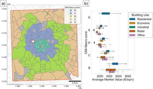
Figure A2. Synthetic datasets of up-down (a) and East-West (b) ground displacement rates derived from the data fusion of PSs resulting from A-DInSAR analyses of S1 and CSK SAR images.

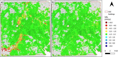
Figure A3. Distribution of building use categories according to single- and multi-risk scores.

References

- Alessi D, Bozzano F, Lisa A, Esposito C, Fantini A, Loffredo A, Martino S, Mele F, Moretto S, Noviello A, et al. 2014. Geological risks in large cities: the landslides triggered in the city of Rome (Italy) by the rainfall of 31 January-2 February 2014. Ital J Eng Geol Environ. 15–34. doi: 10.4408/IJEGE.2014-01.O-02.
- Amanti M, Cesi C, Vitale V. 2008. Le frane nel territorio di Roma -Dal centro storico alla periferia. Descr Carta Geol. d'Italia. 80:83–117.
- Annual Report. 2022. Munich Re; [ accessed 2023 Jun 20]. https://www.munichre.com/en/company/investors/reports-and-presentations/annual-report.html.
- Bell R, Glade T. 2004. Quantitative risk analysis for landslides – examples from Bíldudalur, NW-Iceland. Nat Hazards Earth Syst Sci. 4(1):117–131. doi: 10.5194/nhess-4-117-2004.
- Bianchi Fasani G, Bozzano F, Cercato M. 2011. The underground cavity network of south-eastern Rome (Italy): an evolutionary geological model oriented to hazard assessment. Bull Eng Geol Environ. 70(4):533–542. doi: 10.1007/s10064-011-0360-0.
- Bianchini S, Solari L, Casagli N. 2017. A GIS-based procedure for landslide intensity evaluation and specific risk analysis supported by persistent scatterers interferometry (PSI). Remote Sens. 9(11):1093. doi: 10.3390/rs9111093.
- Bozzano F, Andreucci A, Gaeta M, Salucci R. 2000. A geological model of the buried Tiber River valley beneath the historical centre of Rome. Bull Eng Geol Env. 59(1):1–21. doi: 10.1007/s100640000051.
- Bozzano F, Esposito C, Franchi S, Mazzanti P, Perissin D, Rocca A, Romano E. 2015a. Analysis of a subsidence process by integrating geological and hydrogeological modelling with satellite InSAR data. In: lollino G, Manconi A, Guzzetti F, Culshaw M, Bobrowsky P, Luino F, editors. Engineering geology for society and territory - volume 5. Cham: Springer International Publishing; p. 155–159. doi: 10.1007/978-3-319-09048-1_31.
- Bozzano F, Esposito C, Franchi S, Mazzanti P, Perissin D, Rocca A, Romano E. 2015b. Understanding the subsidence process of a quaternary plain by combining geological and hydrogeological modelling with satellite InSAR data: the Acque Albule Plain case study. Remote Sens Environ. 168:219–238. doi: 10.1016/j.rse.2015.07.010.
- Bozzano F, Esposito C, Mazzanti P, Patti M, Scancella S. 2018. Imaging multi-age construction settlement behaviour by advanced SAR interferometry. Remote Sens. 10(7):1137. doi: 10.3390/rs10071137.
- Brabb EE. 1984. Innovative approaches to landslide hazard and risk mapping. In: Proceedings of the 4th International Symposium on Landslides; Toronto, Canada. Japan Landslide Society. Vol. 1, p. 307–324.
- Caleca F, Tofani V, Segoni S, Raspini F, Rosi A, Natali M, Catani F, Casagli N. 2022. A methodological approach of QRA for slow-moving landslides at a regional scale. Landslides. 19(7):1539–1561. doi: 10.1007/s10346-022-01875-x.
- Campolunghi MP, Capelli G, Funiciello R, Lanzini M. 2007. Geotechnical studies for foundation settlement in Holocenic alluvial deposits in the City of Rome (Italy). Eng Geol. 89(1-2):9–35. doi: 10.1016/j.enggeo.2006.08.003.
- Cascini L. 2008. Applicability of landslide susceptibility and hazard zoning at different scales. Eng Geol. 102(3-4):164–177. doi: 10.1016/j.enggeo.2008.03.016.
- Chang L, Hanssen RF. 2014. Detection of cavity migration and sinkhole risk using radar interferometric time series. Remote Sens Environ. 147:56–64. doi: 10.1016/j.rse.2014.03.002.
- Cigna F, Lasaponara R, Masini N, Milillo P, Tapete D. 2014. Persistent scatterer interferometry processing of COSMO-SkyMed StripMap HIMAGE time series to depict deformation of the historic centre of Rome, Italy. Remote Sens. 6(12):12593–12618. doi: 10.3390/rs61212593.
- Ciotoli G, Di Loreto E, Finoia MG, Liperi L, Meloni F, Nisio S, Sericola A. 2016. Sinkhole susceptibility, Lazio Region, central Italy. J Maps. 12(2):287–294. doi: 10.1080/17445647.2015.1014939.
- Ciotoli G, Loreto E, Liperi L, Meloni F, Nisio S, Sericola A. 2014. Carta dei Sinkhole Naturali del Lazio 2012 e sviluppo futuro del Progetto Sinkholes Regione Lazio. Mem Descr Carta Geol. 99:189–202.
- Cleveland RB, Cleveland WS, McRae JE, Terpenning I. 1990. STL: a seasonal-trend decomposition. J Off Stat. 6(1):3–73.
- Corominas J, van Westen C, Frattini P, Cascini L, Malet J-P, Fotopoulou S, Catani F, Van Den Eeckhaut M, Mavrouli O, Agliardi F, et al. 2013. Recommendations for the quantitative analysis of landslide risk. Bull Eng Geol Environ. 73(2):209–263. doi: 10.1007/s10064-013-0538-8.
- Costantini M, Ferretti A, Minati F, Falco S, Trillo F, Colombo D, Novali F, Malvarosa F, Mammone C, Vecchioli F, et al. 2017. Analysis of surface deformations over the whole Italian territory by interferometric processing of ERS, Envisat and COSMO-SkyMed radar data. Remote Sens Environ. 202:250–275. doi: 10.1016/j.rse.2017.07.017.
- Costantini M, Minati F, Trillo F, Ferretti A, Novali F, Passera E, Dehls J, Larsen Y, Marinkovic P, Eineder M, et al. 2021. European ground motion service (EGMS). In: 2021 IEEE International Geoscience and Remote Sensing Symposium IGARSS, Brussels, Belgium. p. 3293–3296. doi: 10.1109/IGARSS47720.2021.9553562.
- Costantini M, Zhu M, Huang S, Bai S, Cui J, Minati F, Vecchioli F, Jin D, Hu Q. 2018. Automatic detection of building and infrastructure instabilities by spatial and temporal analysis of Insar measurements. In: IGARSS 2018 - 2018 IEEE International Geoscience and Remote Sensing Symposium, Valencia, Spain. p. 2224–2227. doi: 10.1109/IGARSS.2018.8518270.
- Crosetto M, Solari L, Balasis-Levinsen J, Bateson L, Casagli N, Frei M, Oyen A, Moldestad DA, Mróz M. 2021. Deformation monitoring at European scale: the Copernicus ground motion service. Int Arch Photogramm Remote Sens Spatial Inf Sci. XLIII-B3-2021:141–146. doi: 10.5194/isprs-archives-XLIII-B3-2021-141-2021.
- Delgado Blasco JM, Foumelis M, Stewart C, Hooper A. 2019. Measuring urban subsidence in the Rome Metropolitan Area (Italy) with sentinel-1 SNAP-StaMPS persistent scatterer interferometry. Remote Sensing. 11(2):129. doi: 10.3390/rs11020129.
- Del Monte M, D’Orefice M, Luberti GM, Marini R, Pica A, Vergari F. 2016. Geomorphological classification of urban landscapes: the case study of Rome (Italy). J Maps. 12(sup1):178–189. doi: 10.1080/17445647.2016.1187977.
- Dilley M. 2005. Natural disaster hotspots: a global risk analysis. [place unknown]: World Bank Publications.
- Esposito C, Belcecchi N, Bozzano F, Brunetti A, Marmoni GM, Mazzanti P, Romeo S, Cammillozzi F, Cecchini G, Spizzirri M. 2021. Integration of satellite-based A-DInSAR and geological modeling supporting the prevention from anthropogenic sinkholes: a case study in the urban area of Rome. Geomatics Nat Hazards Risk. 12(1):2835–2864. doi: 10.1080/19475705.2021.1978562.
- Esposito C, Mastrantoni G, Marmoni GM, Antonielli B, Caprari P, Pica A, Schilirò L, Mazzanti P, Bozzano F. 2023. From theory to practice: optimisation of available information for landslide hazard assessment in Rome relying on official, fragmented data sources. Landslides. 20[(10):2055–2073. doi: 10.1007/s10346-023-02095-7.
- Fell R, Corominas J, Bonnard C, Cascini L, Leroi E, Savage WZ. 2008. Guidelines for landslide susceptibility, hazard and risk zoning for land-use planning. Eng Geol. 102(3-4):99–111. doi: 10.1016/j.enggeo.2008.03.014.
- Ferretti A, Fumagalli A, Passera E, Rucci A. 2022. Insar data calibration in wide area processing. In: IGARSS 2022 - 2022 IEEE International Geoscience and Remote Sensing Symposium, Kuala Lumpur, Malaysia. p. 5101–5104. doi: 10.1109/IGARSS46834.2022.9884822.
- Ferretti A, Prati C, Rocca F. 2001. Permanent scatterers in SAR interferometry. IEEE Trans Geosci Remote Sensing. 39(1):8–20. doi: 10.1109/36.898661.
- Festa D, Bonano M, Casagli N, Confuorto P, De Luca C, Del Soldato M, Lanari R, Lu P, Manunta M, Manzo M, et al. 2022. Nation-wide mapping and classification of ground deformation phenomena through the spatial clustering of P-SBAS InSAR measurements: Italy case study. ISPRS J Photogramm Remote Sens. 189:1–22. doi: 10.1016/j.isprsjprs.2022.04.022.
- Frankenberg E, Sikoki B, Sumantri C, Suriastini W, Thomas D. 2013. Education, vulnerability, and resilience after a natural disaster. E&S. 18(2):16. doi: 10.5751/ES-05377-180216.
- Giampaolo V, Capozzoli L, Grimaldi S, Rizzo E. 2016. Sinkhole risk assessment by ERT: The case study of Sirino Lake (Basilicata, Italy). Geomorphology. 253:1–9. doi: 10.1016/j.geomorph.2015.09.028.
- Gill JC, Duncan M, Ciurean R, Smale L, Stuparu D, Schlumberger J, de Ruiter M, Tiggeloven T, Torresan S, Gottardo S, et al. 2022. D1.2 Handbook of multi-hazard, multi-risk definitions and concepts [Internet]; [accessed 2023 Jun 18]. https://nora.nerc.ac.uk/id/eprint/533237/.
- Greiving S. 2006. Integrated risk assessment of multi-hazards: a new methodology. Spcl Pap Geol Surv Finland. 42:75.
- Guglielmino F, Nunnari G, Puglisi G, Spata A. 2011. Simultaneous and integrated strain tensor estimation from geodetic and satellite deformation measurements to obtain three-dimensional displacement maps. IEEE Trans Geosci Remote Sensing. 49(6):1815–1826. doi: 10.1109/TGRS.2010.2103078.
- Guzzetti F. 2000. Landslide fatalities and the evaluation of landslide risk in Italy. Eng Geol. 58(2):89–107. doi: 10.1016/S0013-7952(00)00047-8.
- Hanssen RF. 2001. Radar Interferometry: data Interpretation and Error Analysis. [place unknown]: Springer Science & Business Media.
- Hochrainer-Stigler S, Šakić Trogrlić R, Reiter K, Ward PJ, de Ruiter MC, Duncan MJ, Torresan S, Ciurean R, Mysiak J, Stuparu D, et al. 2023. Toward a framework for systemic multi-hazard and multi-risk assessment and management. iScience. 26(5):106736. doi: 10.1016/j.isci.2023.106736.
- https://www.sarinterferometry.com/ps-toolbox/. SAR PS ToolBox [Internet]; [accessed 2023 Jul 26]. NHAZCA S.r.l.
- Huang B, Shu L, Yang YS. 2012. Groundwater overexploitation causing land subsidence: hazard risk assessment using field observation and spatial modelling. Water Resour Manage. 26(14):4225–4239. doi: 10.1007/s11269-012-0141-y.
- Huang S, Dou H, Jian W, Guo C, Sun Y. 2023. Spatial prediction of the geological hazard vulnerability of mountain road network using machine learning algorithms. Geomatics Nat Hazards Risk. 14(1):2170832. doi: 10.1080/19475705.2023.2170832.
- Hyndman RJ, Athanasopoulos G. 2018. Forecasting: principles and practice. [place unknown]: OTexts.
- Johnson K, Depietri Y, Breil M. 2016. Multi-hazard risk assessment of two Hong Kong districts. Int J Disaster Risk Reduct. 19:311–323. doi: 10.1016/j.ijdrr.2016.08.023.
- Julià PB, Ferreira TM. 2021. From single- to multi-hazard vulnerability and risk in historic urban areas: a literature review. Nat Hazards. 108(1):93–128. doi: 10.1007/s11069-021-04734-5.
- Kappes MS, Keiler M, von Elverfeldt K, Glade T. 2012b. Challenges of analyzing multi-hazard risk: a review. Nat Hazards. 64(2):1925–1958. doi: 10.1007/s11069-012-0294-2.
- Kappes MS, Papathoma-Köhle M, Keiler M. 2012a. Assessing physical vulnerability for multi-hazards using an indicator-based methodology. Appl Geogr. 32(2):577–590. doi: 10.1016/j.apgeog.2011.07.002.
- Komendantova N, Mrzyglocki R, Mignan A, Khazai B, Wenzel F, Patt A, Fleming K. 2014. Multi-hazard and multi-risk decision-support tools as a part of participatory risk governance: feedback from civil protection stakeholders. Int J Disaster Risk Reduct. 8:50–67. doi: 10.1016/j.ijdrr.2013.12.006.
- Li Z, Nadim F, Huang H, Uzielli M, Lacasse S. 2010. Quantitative vulnerability estimation for scenario-based landslide hazards. Landslides. 7(2):125–134. doi: 10.1007/s10346-009-0190-3.
- Liu X, Chen H. 2019. Integrated assessment of ecological risk for multi-hazards in Guangdong province in Southeastern China. Geomatics Nat Hazards Risk. 10(1):2069–2093. doi: 10.1080/19475705.2019.1680450.
- Liu Z, Nadim F, Garcia-Aristizabal A, Mignan A, Fleming K, Luna BQ. 2015. A three-level framework for multi-risk assessment. Georisk. 9(2):59–74. doi: 10.1080/17499518.2015.1041989.
- Luo H, Chen T. 2016. Three-dimensional surface displacement field associated with the 25 April 2015 Gorkha, Nepal, earthquake: solution from integrated InSAR and GPS measurements with an extended SISTEM approach. Remote Sens. 8(7):559. doi: 10.3390/rs8070559.
- Marzocchi W, Garcia-Aristizabal A, Gasparini P, Mastellone ML, Di Ruocco A. 2012. Basic principles of multi-risk assessment: a case study in Italy. Nat Hazards. 62(2):551–573. doi: 10.1007/s11069-012-0092-x.
- Mastrantoni G, Marmoni GM, Esposito C, Bozzano F, Scarascia Mugnozza G, Mazzanti P. 2023. Reliability assessment of open-source multiscale landslide susceptibility maps and effects of their fusion. Georisk. 0(0):1–18. doi: 10.1080/17499518.2023.2251139.
- McGlade J, Bankoff G, Abrahams J, Cooper-Knock SJ, Cotecchia F, Desanker P, Erian W, Gencer E, Gibson L, Girgin S. 2019. Global assessment report on disaster risk reduction 2019. Geneva, Switzerland: UN Office for Disaster Risk Reduction (UNDRR).
- Mohebbi Tafreshi G, Nakhaei M, Lak R. 2021. Land subsidence risk assessment using GIS fuzzy logic spatial modeling in Varamin aquifer, Iran. GeoJournal. 86(3):1203–1223. doi: 10.1007/s10708-019-10129-8.
- Papathoma-Köhle M, Neuhäuser B, Ratzinger K, Wenzel H, Dominey-Howes D. 2007. Elements at risk as a framework for assessing the vulnerability of communities to landslides. Nat Hazards Earth Syst Sci. 7(6):765–779. doi: 10.5194/nhess-7-765-2007.
- Pedregosa F, Varoquaux G, Gramfort A, Michel V, Thirion B, Grisel O, Blondel M, Prettenhofer P, Weiss R, Dubourg V, et al. 2011. "Scikit-learn: Machine Learning in Python". J Mach Learn Res. 12:2825–2830.
- Romão X, Paupério E, Pereira N. 2016. A framework for the simplified risk analysis of cultural heritage assets. J Cult Heritage. 20:696–708. doi: 10.1016/j.culher.2016.05.007.
- Shi Y, Tang Y, Lu Z, Kim J-W, Peng J. 2019. Subsidence of sinkholes in Wink, Texas from 2007 to 2011 detected by time-series InSAR analysis. Geomatics Nat Hazards Risk. 10(1):1125–1138. doi: 10.1080/19475705.2019.1566786.
- Terzi S, Torresan S, Schneiderbauer S, Critto A, Zebisch M, Marcomini A. 2019. Multi-risk assessment in mountain regions: a review of modelling approaches for climate change adaptation. J Environ Manage. 232:759–771. doi: 10.1016/j.jenvman.2018.11.100.
- Tilloy A, Malamud BD, Winter H, Joly-Laugel A. 2019. A review of quantification methodologies for multi-hazard interrelationships. Earth Sci Rev. 196:102881. doi: 10.1016/j.earscirev.2019.102881.
- UNISDR W. 2012. Disaster risk and resilience. Thematic Think Piece, UN System Task Force on the Post-2015 UN development agenda. Technical Report, United Nations.
- van Westen C, Kappes MS, Luna BQ, Frigerio S, Glade T, Malet J-P. 2014. Medium-scale multi-hazard risk assessment of gravitational processes. In: Van Asch T, Corominas J, Greiving S, Malet J-P, Sterlacchini S, editors. Mountain risks: from prediction to management and governance. Dordrecht: Springer Netherlands. p. 201–231. doi: 10.1007/978-94-007-6769-0_7.
- Varnes DJ. 1984. Landslide hazard zonation: a review of principles and practice. Nat Hazards. No. 3:63.
- Ward PJ, Blauhut V, Bloemendaal N, Daniell JE, de Ruiter MC, Duncan MJ, Emberson R, Jenkins SF, Kirschbaum D, Kunz M, et al. 2020. Review article: natural hazard risk assessments at the global scale. Nat Hazards Earth Syst Sci. 20(4):1069–1096. doi: 10.5194/nhess-20-1069-2020.
- Wei L, Hu K, Hu X, Wu C, Zhang X. 2022. Quantitative multi-hazard risk assessment to buildings in the Jiuzhaigou valley, a world natural heritage site in Western China. Geomatics Nat Hazards Risk. 13(1):193–221. doi: 10.1080/19475705.2021.2004244.
- White GF, Kates RW, Burton I. 2001. Knowing better and losing even more: the use of knowledge in hazards management. Global Environ Change Part B Environ Hazards. 3(3-4):81–92. doi: 10.3763/ehaz.2001.0308.
- Zisman ED. 2008. A method of quantifying sinkhole risk. In: Sinkholes and the Engineering and Environmental Impacts of Karst. p.278–287. doi: 10.1061/41003(327)27.