Investigating kinematics and triggers of slow-moving reservoir landslide using an improved MT-InSAR method

Abstract

The safety of the Three Gorges Reservoir, the world’s largest hydraulic project, has attracted significant attention. Among the landslides in the area, the Xinpu landslide complex stands out as one of the largest. However, accurately detecting and interpreting the timing and magnitude of its movement remains a challenge. This study introduces a framework using interferometric synthetic aperture radar (InSAR) for investigating the Xinpu landslide complex. In areas with dense vegetation like Xinpu, estimating landslide movement has traditionally been problematic. The proposed method, based on independent component analysis-assisted intermittent multi-temporal InSAR, overcomes this limitation by retrieving complete and reliable time-series deformation without prior deformation models. Through an analysis of Sentinel-1 datasets covering a period of 4 years, our approach significantly enhances deformation density and accuracy in comparison to other multi-temporal InSAR techniques. When contrasted with these methods, our proposed approach exhibits an average RMS improvement of up to 46.2% between GNSS measurements and the InSAR-derived results. The complete time-series deformation reveals diverse triggers at different sections of the Xinpu landslide complex. Precipitation, with a 45-day lag, primarily controls the landslide, while the toe of the landslide shows joint effects from precipitation and water level fluctuations, with a 14-day lag. Cross-correlation analysis estimates lag times for deformation responses to different triggers and enables discussion of the complex’s kinematic process. Overall, this approach enhances InSAR performance in vegetated areas and aids in uncovering landslide triggers for effective hazard mitigation.

Keywords:

• Reservoir landslide
• interferometric synthetic aperture radar (InSAR)
• independent component analysis (ICA)
• xinpu landslide complex
• landslide kinematics

1. Introduction

Landslides are a mass-wasting process caused by the raised ratio of failure shear stress to resisting shear strength; landslides have affected many areas worldwide and often cause catastrophic consequences (Petley 2012). As a special type of site suffering from landslides, the reservoir bank slope is affected by the regular operation of a hydropower station. The impoundment and discharge cycle of the reservoir, together with other triggers, such as rainfall or road construction, usually decrease slope stability (Paronuzzi et al. 2013). Three Gorges Reservoir (TGR) is the biggest hydraulic project in the world. The complicated geologic environment, widespread unstable slopes, and large fluctuations of the bank water level often induce serious landslide disasters, such as the Qianjiangping landslide on July 13, 2003 (Wang et al. 2004), the Gongjiafang landslide on November 23, 2008 (Huang et al. 2012), and the Hongyanzi landslide on June 24, 2015 (Wang et al. 2019).

Comprehensive deformation monitoring helps in understanding how landslide movements evolve with time, how the mass moves in space, and what their driving factors are. Over the past two decades, interferometric synthetic aperture radar (SAR, InSAR) has played an important role in the monitoring of landslide deformations with its high-precision, large-coverage, and frequent-acquisition features (Colesanti and Wasowski 2006; Bayer et al. 2017; Intrieri et al. 2017; Hu et al. 2020). The archive data provided by SAR satellites enable us to track the history of an unknown landslide (Samsonov et al. 2020; Xiong et al. 2020). Recently, InSAR has been successfully applied in the monitoring of reservoir bank slopes (Shi et al. 2017; Li et al. 2019). Especially, the open-access Sentinel-1 data provide a high-quality, fast-revisited, and stable tool for researchers, further extending the application of InSAR to monitor geohazards.

The TGR area is a high-risk region of landslides, and several studies have been performed with SAR observations to facilitate hazard mitigation (Liao et al. 2011; Singleton et al. 2014; Tomás et al. 2014; Zhou et al. 2020). However, InSAR faces a series of challenges when utilized in the TGR area. First, it is hard to keep high coherence during the long-term time series of SAR observation because of the decorrelation noise induced by the dense vegetation in the TGR area, resulting in a dramatic decrease in the number of measurement points (MPs) (Liao et al. 2011; Tomás et al. 2014). Second, long-wavelength SAR imagery (e.g. ALOS-1/2) has been the most adopted data in the TGR area because of its good penetrability in the vegetation-covered region. However, the time-series deformation results bring difficulties in retrieving the details of temporal behavior because of low time resolution (Shi et al. 2016). If high-time-resolution but short-wavelength data (e.g. Sentinel-1 or TerraSAR-X) are utilized, the number of MPs will be less (Liao et al. 2011; Liu et al. 2013). To improve the defects, corner reflectors (CRs) can be employed to overcome the decorrelation and retrieve the time-series deformation in the TGR area (Singleton et al. 2014; Shi et al. 2015). However, the CRs lower spatial resolution and fail to understand the distribution of deformation.

Mapping landslide movement with spatially complete time-series deformation in the vegetation area is therefore a challenge for monitoring landslides using InSAR. ‘Intermittent MPs’ are a choice to improve the number of MPs, which keep high-coherent pixels for a part of the period rather than the whole period. Several methods have been proposed based on this concept (e.g. TCP-InSAR (Zhang et al. 2011) and ISBAS (Bateson et al. 2015)). However, intermittent MPs will decrease the accuracy of the time-series deformation; therefore, it is a trade-off between the accuracy and spatial coverage of results (Bateson et al. 2015). Unwrapped errors, model bias, and atmospheric artifacts are the main factors that induce the uncertainties of time-series deformation. Independent component analysis (ICA) is a nonparametric technique to retrieve source signals from multiple mixed receivers (Comon 1994; Hyvärinen and Oja 1997). The method derives an independent component by maximizing the statistical independence based on the assumption that each constituent component has a non-Gaussian probability distribution (Ebmeier 2016). Various errors of InSAR observation are expected to be statistically independent in spatial and temporal domains (Ebmeier 2016), which means that the ICA is appropriate for time-series InSAR observation and is, therefore, of benefit for deriving more accurate results from intermittent MPs. In this study, we applied an ICA-assisted intermittent multitemporal InSAR method to derive the spatially complete time-series deformation associated with the Xinpu landslide complex using the Sentinel-1 data during 2016–2020.

The Xinpu landslide complex is a reservoir landslide and is located in the west of the TGR area. As one of the largest landslides in the TGR area, the Xinpu landslide complex brings great threats to the routine operation of the Three Gorges hydropower station and the people living nearby. It is of great significance to derive the spatial–temporal patterns of the Xinpu landslide complex through InSAR measurements and interpret the triggers for further assessing the risk. In this study, a new workflow of MT-InSAR is first designed by utilizing the intermittent MPs, model-free inversion, and outliers detector to enhance the spatial coverage of results. Then, time-series deformation is optimized by utilizing the ICA method to reduce the uncertainties. The derived spatially complete time-series deformation results are validated with the homochromous global navigation satellite system (GNSS) observations and then in tandem with the local hydrology record to analyze the triggers, lag time, and kinematic process of the Xinpu landslide complex.

2. Study area and materials

2.1. Geological setting of the Xinpu landslide complex

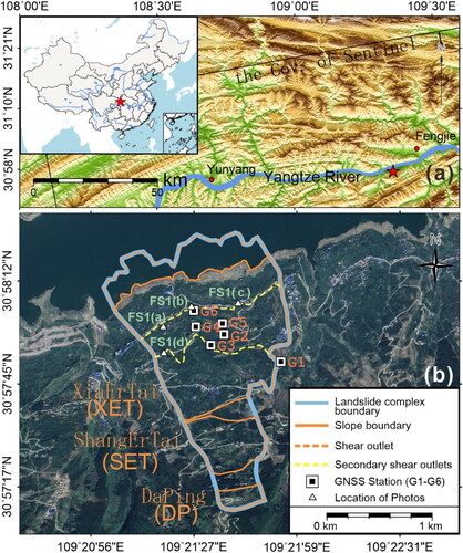
The Xinpu landslide complex is one of the largest landslides in the TGR area, with problems related to the building safety of inhabitants. This landslide complex is about 168 km far from Three Gorges Dam, on the southern shore of the Yangtze River in Fengjie County, Chongqing City, China (Figure 1(a)). The whole slide body extends up to 700 m a.s.l. from 80 m a.s.l., occupying a surface of 2.45 × 10⁶ m² and a volume of 3.998 × 10⁷ m³ (Figure 1(b)) (Jiang et al. 2020). Because the water level of the TGR has increased to 175 m a.s.l. since 2008, the toe of this landslide is submerged under the Yangtze River. Therefore, the impoundment and discharge cycle of TGR may destabilize the Xinpu landslide complex. The fluctuation of the water level in the TGR area has experienced three stages (Tomás et al. 2014). The first rise of the reservoir water level started on June 1, 2003, reaching 135 m a.s.l on June 15, 2003. For the second stage, the water level had increased to 156 m a.s.l on October 27, 2006. The third rise started in November 2008, resulting in the present water level of 175 m a.s.l. After the significant impoundment operation, several potential and old landslides were activated (Li et al. 2019). To guarantee the safety of the Three Gorges Dam, the water level is controlled from 145 to 175 m a.s.l. based on local hydrology changes. The precipitation in the TGR area is divided into the dry season (from October to March) and the wet season (from April to September). Since the heavy rainfall usually couples with the discharge operation, the movement of landslides accelerates in the TGR area during the wet season.

Figure 1. (a) Location of Xinpu landslide complex and coverage of the Sentinel-1 data used (black box), superimposed on the shaded relief map. The Xinpu landslide complex (red star) lies between two major counties (red dots), namely, Fengjie and yunyang. The inset is a sketch map of China. (b) Google Earth image of the Xinpu landslide complex, composed of the XiaErTai (XET) slope (including the submerged area shown as the orange dashed line), ShangErTai (SET) slope, and DaPing (DP) slope. The squares and triangles indicate the locations of GNSS stations and photos in Figure S1, respectively. Landslide outlines are from field survey.

The inception of monitoring activities for the Xinpu landslide can be traced back to March 2007 when Jiang et al. (2020) initiated the deployment of four GPS monitoring stations on the landslide site. During the subsequent reservoir discharge phase following the initial experimental water storage in the Three Gorges Reservoir area, the GPS monitoring findings revealed an absence of significant movements within the Xinpu landslide. In contrast, during the period of low water level operations at the reservoir, spanning from June to September 2007, the Xinpu landslide exhibited marked displacements, underscoring its responsiveness to fluctuations in the reservoir water level. Moreover, the GPS monitoring data also documented a notable acceleration in landslide activity following the occurrence of the Wenchuan earthquake in 2008. According to the GPS monitoring data presented by Jiang et al. (2020), the Xinpu landslide remained in a state of gradual motion between 2007 and 2015. However, a pronounced acceleration in landslide activity emerged during the wet season of 2013, which was attributed to a 15-day intense precipitation in that year. Furthermore, observations derived from underground optical fiber sensors concurred with these findings, demonstrating that landslide movements are more pronounced in years characterized by higher precipitation levels compared to drier years. Additionally, it was evident that dynamic fluctuations in the reservoir water level exerted a discernible influence on the overall stability of the Xinpu landslide (Ye et al. 2023).

Few faults can be found in the Xinpu landslide complex and surrounding areas (Figure 2(a)). According to the geological survey, there are four strata outcropping in the slope: T₃xj, J_1Z, Q₄^col+dl, and Q₄^del (Figure 2(b)). Upper Triassic Xujiahe Formation (T₃xj) comprises carbonaceous shale, silty mudstone, and sandstone. The material composition of the Lower Jurassic Zhenzhuchong Formation (J_1Z) includes lithic quartz sandstone, gray shale, and argillaceous siltstone. The Quaternary Holocene deposits (Q₄^col+dl and Q₄^del) are the main component of the sliding masses. Note that the Quaternary Holocene landslide deposit (Q₄^del) comprises gravel mixed with silty clay (Figure 2(c)). This layer is favorable for the infiltration of surface water due to its large pore spaces, acting as an active seasonal aquifer responsible for slope stability (Seguí et al. 2020; Ye et al. 2022).

Figure 2. Geological setting of the Xinpu landslide complex. (a) Lithologic map with a scale of 1:500,000 showing the geological setting of the surrounding areas (J₁, J₂, J₃: Lower, Middle, and Upper Jurassic strata; T₁, T₂, T₃: Lower, Middle, and Upper Triassic strata; the red region is the study area). (b) Geological plane map of the Xinpu landslide complex. (c) a longitudinal cross-section G-G’ of XET slope showing the inferred limits of different subzones.

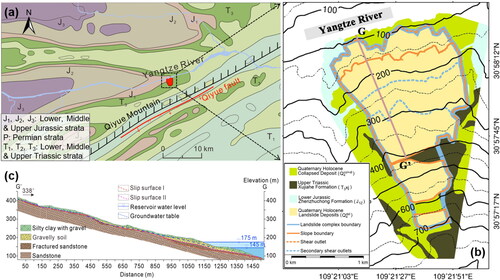
Because landslide movement is controlled by the sliding bed and lithology, the Xinpu landslide complex is formed by three interrelated and independent slumping bodies, i.e. XiaErTai (XET) slope, ShangErTai (SET) slope, and DaPing (DP) slope (Figure 1(b)). The DP slope is located on the upper part of the Xinpu landslide complex, which is in a steady state. The XET slope lies in the lower part of the landslide, and the SET slope is in the middle section of the Xinpu landslide complex. The shear outlet is positioned at the toe of the landslide, as indicated by the orange dashed line in Figure 1(b), and it has become submerged subsequent to the initial phase of reservoir water level rise. Within the XET slope, there exist two secondary shear outlets. The lower one runs parallel to the road, where a retaining wall has been constructed to safeguard both the road and the adjacent buildings in its vicinity, as depicted by the yellow dashed line in Figure 1(b). Based on earlier in situ observations between 2003 and 2006, the XET and SET landslides had suffered obvious surface deformations. Especially, as the largest section of the Xinpu landslide complex with a total volume of 3.41 × 10⁷ m³, the XET slope experienced obvious ground movements, which have caused many cracks in local houses and roads (Figure S1). With long-term movement, two secondary shear outlets were formed in the XET slope (shown as the dashed yellow lines in Figure 1(b)).

2.2. Available materials

Considering that Sentinel-1 can provide fast-revisited and long-term observations, which is beneficial for deriving temporal details, 124 C-band ascending scenes of Sentinel-1 single-look complex data from August 1, 2016, to October 15, 2020, are utilized to retrieve the spatial–temporal pattern of the Xinpu landslide complex. In Figure S1(a), the slope is covered by the dense vegetation, which challenges the procurement of a spatially complete pattern with the C-band SAR dataset. It was also found that the buildings on the slope were greatly damaged (Figure S1(b) and S1(c)). To investigate the stability of the Xinpu landslide complex, six GNSS stations were built at the end of 2019 (the location is shown in Figure 1(b)), among which the G1 station was used as the reference and the G2–G5 stations were used to monitor deformation.

According to previous studies (Shi et al. 2015; Tomás et al. 2015), the reservoir water level and rainfall can be considered triggers that are linked to the stability of the reservoir bank slope in the TGR area. Daily water levels are obtained from January 2014 to November 2020, showing obvious cyclical changes due to flooding control measures. Rainfall records are also available from the meteorological station at Fengjie with a time step of 1 day, representing an obvious seasonality due to monsoons. These records were collected and adopted to interpret the mechanism of the movements of the Xinpu landslide complex.

3. Methodology

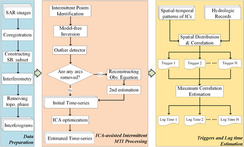
To obtain the spatially complete time-series deformation pattern and the kinematic process of a slow-moving landslide, we have designed a workflow, which includes the process of ICA-assisted intermittent multi-temporal InSAR analysis method, and the derivation of the triggers and corresponding lag time. Our method includes four steps, i.e. the identification of intermittent points, model-free inversion, outliers detection, and ICA postprocessing. With independent components derived by ICA, various triggers can be identified, and then the lag time can be estimated to understand the kinematic process of the Xinpu landslide. The flowchart is illustrated in Figure 3. In the next sections, we will describe these steps in detail.

Figure 3. Flowchart of the implemented method.

3.1. Data preparation

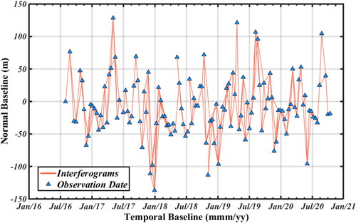
A consistent dataset of differential SAR interferograms with a stack of Sentinel-1 data was generated following the workflow in Figure 3 (the blue box). Orbit state vectors of Sentinel-1 data were first improved by utilizing the precise orbit ephemerides obtained from the Sentinel-1 quality control subsystem, which minimizes orbital errors. Considering the impacts of decorrelation in the vegetation area, thresholds of 36 days temporal intervals and 180-m perpendicular baselines were utilized to select the short-baseline (SB) interferometric pairs after coregistered processing (Figure 4). Several pairs of interferograms with low coherence were removed, and we then obtained 223 interferograms for further time-series processing. To improve coherence, multi-look numbers of 5 × 1 (range × azimuth) were adopted to generate the interferograms, and the slant range and azimuth pixel spacing of the scenes were ∼14 m, which corresponded nominally to ∼20 m on the ground. We subtracted the topographic phase from interferograms with 1 arc-second resolution Shuttle Radar Topography Mission (SRTM) Digital Elevation Model (DEM), and the differential interferograms were then obtained.

Figure 4. Spatial and temporal baselines of the generated interferometric pairs from 124 Sentinel-1 scenes.

Although a short temporal baseline was utilized to avoid the severe temporal decorrelation, the fast-growing vegetation still led to many invalid MPs in a proportion of interferograms, which would result in an incomplete deformation field, and degraded the reliability of the derived spatial–temporal patterns. In particular, because more than 200 interferograms from more 4-year observations were adopted in this study, it was difficult to obtain high-quality MPs in each interferogram.

3.2. ICA-assisted intermittent MT-InSAR processing

The ICA-Assisted Intermittent MT-InSAR method is developed to improve the density of MPs in the Xinpu landslide complex. This method estimates time-series deformation with intermittent MPs, which do not require the MPs to retain high coherence in the whole period; therefore, the density of MPs can be increased. The main processing flow of our method is designed as follows.

• Step 1: the intermittent points are identified with a threshold of mean coherence, and then the identified MPs are connected by the Delaunay triangulation to form arc phase.

• Step 2: the initial time series is estimated by the model-free inversion and outliers detector to contain all the deformation signals and avoid phase unwrapping errors.

• Step 3: if any arcs are removed, reconstruct the observation equation with the residual arcs, and then the time series will be re-estimated.

• Step 4: the FastICA algorithm is utilized to derive the multiple independent components from the initial time series, and then the time series can be derived by combining the identified components.

The detailed processing of our method is described further in follows.

Because the distributed scatters are overwhelmingly available in mountainous areas, the coherence of interferograms was adopted as the criterion to select the MPs. Herein, we set 0.2 as the threshold of mean coherence to identify the MPs, and 96,788 MPs were identified, which cover all of the Xinpu landslide complex. Unwrapped error is a major effect that decreases the precision of the time series in landslide monitoring. Therefore, we employed Delaunay triangulation to establish connections between the phases of MPs with short baselines, referring to each connected pair as an 'arc’ (Sousa et al. 2011). Utilizing arc phase when processing time-series InSAR data proves advantageous in mitigating phase discontinuities, especially in complex mountainous terrains (Zhang et al. 2018). Further, 409,580 arcs were constructed between the selected MPs.

The intermittent MPs decrease the reliability of the time series and are usually a tradeoff between the accuracy and spatial coverage of the results (Bateson et al. 2015). Atmospheric phase screen (APS), residual topography, model bias, and unwrapped errors are the main factors that induce uncertainty in deriving accurate deformation of landslides. ICA is a powerful tool for deriving independent components from mixed signals. However, time-series deformation is usually derived with the prior model (e.g. linear model or periodic model) in the workflow of most conventional MT-InSAR methods, which may ignore a portion of deformation signals. To retain all the deformation signals and avoid model bias, we utilize a model-free method to estimate the sequential phase in the time series instead of fitting the deformation with the prior model. Considering $N+1$ SAR images obtained in a time sequence $(\begin{array}{cccc}{t}_0& t_1& \dots & t_N\end{array}),$ $M$ interferograms with short baselines are generated. For each interferogram $i,$ the line-of-sight (LOS) displacement $\Delta r_{i,k}$ at the arc $k$ can be expressed as (1) $$\Delta r_{i,k}=\sum _{j=t_p}^{t_s}(t_j-t_{j-1})\Delta v_{i,k},$$(1) where $\Delta v_{i,k}$ is the deformation velocity from the acquisition of the primary image $t_p$ to that of the secondary image $t_s.$ The phase of selected interferograms $\Delta R_k$ at arc $k$ can be written as (2) $$\Delta R_k=-\frac{4\pi }{\lambda }\cdot B\cdot \Delta V_k,$$(2) where $B$ is a $M\times N-1$ design matrix, which represents the interval in each interferogram and $\Delta V_k={\left[\begin{array}{cccc}\Delta v_{1,k}& \Delta v_{2,k}& \dots & \Delta v_{N,k}\end{array}\right]}_{N\times 1}$ are the sequential velocities in an ordered time sequence, which can be solved with the least square estimator.

Although the arcs in the SB interferograms have been adopted to avoid the wrapped phase, arcs could include phase ambiguities in some interferograms during the first least square estimation. The arcs with ambiguities can be detected and eliminated by implementing an outlier detector. The outlier detector is applied through the residual phase $\Delta {\mathit{\Phi }}_{\mathit{res},k},$ which can be estimated with (Zhang et al. 2011) (3) $$\Delta {\mathit{\Phi }}_{\mathit{res},k}=-\frac{4\pi }{\lambda }\cdot B\cdot \Delta {\widehat{V}}_k-\Delta R_k.$$(3) where $\Delta {\widehat{V}}_k$ is the estimated sequential velocities via Eq. (2)(2) $$\Delta R_k=-\frac{4\pi }{\lambda }\cdot B\cdot \Delta V_k,$$(2) . Then, the outlier detector can be implemented using (Zhang et al. 2011) (4) $$\max \left(\right|\Delta {\mathit{\Phi }}_{\mathit{res},k}\left|\right)=c\sqrt{\mathrm{m}\mathrm{ax}\left({\left(Q^{dd}\right)}_k\right)}+2\sqrt{\mathrm{m}\mathrm{ax}\left({\left(Q_{\Delta \mathit{\Phi }\Delta \mathit{\Phi }}\right)}_k\right)},$$(4) where $Q^{dd}$ and $Q_{\Delta \mathit{\Phi }\Delta \mathit{\Phi }}$ can be estimated using $Q^{dd}=2\cdot B\cdot B^T$ and $Q_{\Delta \mathit{\Phi }\Delta \mathit{\Phi }}=B\cdot {(B^T\cdot B)}^{-1}{B}^T,$ respectively. $\max (\cdot )$ is the maximum value in the matrix. $c$ is a constant and can be chosen as 3 or 4 (Zhang et al. 2011).

After applying the outlier detector, a portion of the arcs are removed. To obtain more MPs for deriving the spatially complete patterns, the temporary arcs are also implemented to solve the final solution based on the rank of the new design matrix $\mathit{rank}(B^{\prime }),$ where $B^{\prime }$ is a reconstructed design matrix based on the residual interferograms after applying the outlier detector. Specifically, if no arcs are removed after applying the outlier detector in a pair of MPs, the time-series deformation of the pair of MPs is directly retrieved. When some arcs are removed, we will replace the design matrix $B$ with $B^{\prime }$ in Eq. (2)(2) $$\Delta R_k=-\frac{4\pi }{\lambda }\cdot B\cdot \Delta V_k,$$(2) . The rank of the new design matrix is then estimated. Once $\mathit{rank}(B^{\prime })\ge N,$ Eq. (2)(2) $$\Delta R_k=-\frac{4\pi }{\lambda }\cdot B\cdot \Delta V_k,$$(2) will be solved with a least-square (LS) estimator again and the initial time-series deformation will be retrieved with the residual arcs. These processes do not require the arcs to maintain the high quality during the whole observation period, which is beneficial for avoiding the discontinuous subset in the coherent point network and obtaining more dense MPs. After all the time-series deformations of arcs are estimated in arcs, the landslide time-series deformation can be retrieved through a design matrix that links the arcs and points (Zhang et al. 2011).

Although the intermittent points are helpful for deriving the spatially complete patterns, the time series may be affected by severe noise in intermittent MPs, which cannot provide the reliable temporal behavior of the movement. To further improve the initial time series, we implement the FastICA approach as a postprocessing algorithm (Hyvärinen and Oja 1997). This method derives the independent components through the centering, whitening, and fixed-point iteration steps (Hyvarinen 1999; Hyvärinen and Oja 2000), and has been widely used in the geophysical field (Karimzadeh et al. 2018; Peng et al. 2022), more implementation details are provided in the supporting information (see Text S1). After implementing the FastICA postprocessing, seven source matrices $S$ and mixing matrices $A$ can be obtained, which represent the temporal and spatial characteristics of corresponding independent components (ICs), respectively (as shown in Figure S2). With the spatial-temporal patterns of ICs, $n$ components can be identified as the signals of landslide movements. Then, the mixing and source matrices of movement components are combined to obtain the time-series deformation using. (5) $$D=\sum _{i=1}^n{A}_i\otimes S_i,$$(5) where $D$ is the spatially complete time-series deformation of landslide, $\otimes$ is the Kronecker product. The derived landslide time-series deformation can overcome the effects of the hard-modeling noise in intermittent MPs and provide a reliable temporal behavior of landslides, which is helpful for studying the process of the Xinpu landslide complex.

3.3. Triggers and lag time estimation

Triggers are critical for understanding the mechanism of the landslide. Different sections of a landslide usually show distinct movement patterns even at the same time (e.g. the Pianello landslide in Italy (Wasowski and Pisano 2019) and the Huangtupo landslide in the TGR area (Tomás et al. 2015)). Spatially complete time-series deformation provides the possibility for deriving the triggers in different sections. Herein, after implementing the ICA, the eigenvectors and corresponding scores can be derived, which can be regarded as the spatial-temporal deformation pattern induced by different triggers. The spatial distribution of triggers’ effects can be identified from the scores. Besides, we normalize the IC eigenvectors and compare them with the possible driving factors. Because the hydrology factors of the reservoir are the main triggers for a reservoir bank slope landslide (Shi et al. 2015; Li et al. 2018; Xu and Niu 2018), the precipitation and reservoir water level records were adopted to compare with the normalized IC eigenvectors. The comparison is implemented with cross-correlation processing. To quantify the effects of corresponding triggers, the lag time is estimated. With long-term temporal behavior, the lag time of corresponding triggers can be estimated by the cross-correlation (Cohen-Waeber et al. 2018). In this study, we estimate a series of correlations coefficient through a 1-day sliding window, the step with the maximum correlation is regarded as the lag time.

4. Results

4.1. Spatial–temporal patterns of the Xinpu landslide complex

The movement of the Xinpu landslide complex usually accelerates in the summer, which has caused damage to a few buildings (Figure S1). In this study, a spatially complete time-series deformation was derived based on the proposed method (Figure 5), which is crucial for understanding landslides.

Figure 5. Spatial–temporal pattern of the Xinpu landslide complex. (a) LOS deformation rate field derived using our method. The background is a three-dimensional model derived from SRTM DEM. (b–c) Time-series accumulative displacements (colorful lines) and elevation (gray areas) along (b) P–P′, (c) a–a′, and (d) B–B′ profiles.

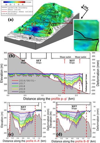
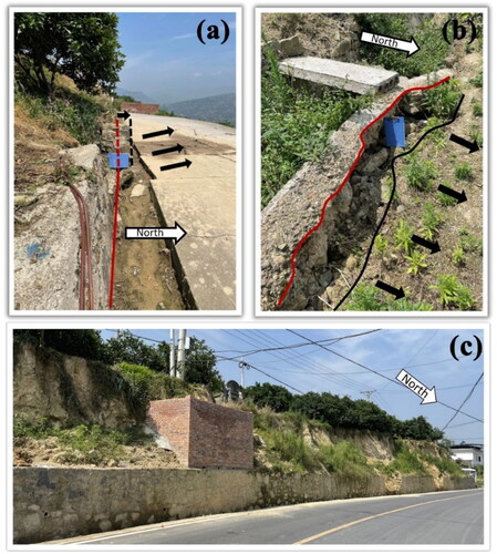
According to the derived spatially complete deformation field, there are no obvious movements in the DP slope, which means that it was in a stable state. Most deformation areas are distributed in the XET slope with a maximum LOS rate of 73 mm/yr (Figure 5(a)). In the boundary between the SET and XET slopes, a mini kinematic unit is detected in the derived spatially complete deformation field (Figure 5(a), the red circle). Although the maximum LOS rate of this kinematic unit is just achieved at 34 mm/yr, considering that the aspect of the Xinpu landslide complex is near parallel to the heading of the satellite, the actual deformation should be larger. This is validated by field investigations. An obvious movement in the mini kinematic unit was found (Figure 6(a)), which had led the retaining wall to move more than 200 mm, causing many obvious cracks in the ground.

Figure 6. Photos from the field investigation. (a) Mini kinematic unit, which is observed in the derived spatial pattern. (b & c) The secondary shear outlets of L1 and L2 in Figure 5(a).

With the spatially complete deformation field, it can be observed that the deformation in the Xinpu landslide complex did not extend from the center to the toe of the landslide and was distributed in the center of the XET slope. To find the reasons for this phenomenon, a profile is set across the Xinpu landslide complex, where the time-series accumulated displacements and elevation are extracted (Figure 5(b)). The deformation increased from the upper to the middle of the XET slope and then decreases until the time-series accumulated deformation achieved the bottom at L2, where there was a secondary shear outlets (Figure 5(a), the red line). A similar phenomenon is found at L1, where the deformation suddenly decreased. Based on the field investigation, a few obvious cracks and shear outlets were observed in L1 and L2 (Figure 6(b,c)). The shear outlet in L1 had pulled the ground apart and caused a significant crack. Furthermore, it is worth noting the presence of a retaining wall constructed along L2 (Figure 6(c)). This retaining wall serves the purpose of safeguarding both the road and the adjacent buildings on either side of it. Therefore, one can anticipate that the primary contributors to obstructing the extent of deformation from the central region of the XET slope to the reservoir bank’s periphery are the secondary shear outlets and the accompanying retaining wall. After L2, the displacement steadily rose again. Additionally, we extracted the time-series accumulated deformation along with the profiles A-A′ and B-B′ for further analyzing the spatial–temporal deformation pattern of this slope. It is observed that the time-series accumulated deformation is symmetric and larger in the middle of profiles A-A′ and B-B′, and the derived boundary of deformation is slightly shorter than that in previous field investigation (Figure 5(c,d), the dashed red lines).

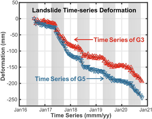
Figure 5(b–d) shows that the cumulative LOS movements increased rapidly in 2017 and 2020. The area with the maximum increase of deformation is in the center of the XET slope, which caused severe damage to buildings (Figure S2(b,c)), and the maximum cumulative LOS deformation achieved is 249 mm. Figure 7 provides more details regarding the temporal behavior of the Xinpu landslide complex. It can be found that the movement of the Xinpu landslide complex always begins to accelerate during the wet season of each year (Figure 7, the gray areas), and then the trend of accelerated displacement decreases during the dry season. The initial period of accelerated movement within the observation timeframe was identified in 2017, showcasing a peak cumulative LOS deformation of approximately 90 mm. The accelerated movement continued for a short time after the wet season. In 2018 and 2019, the accelerated movement was slower than that in 2017. However, the accelerated movement became obvious again in 2020 and led to a series of damages. The triggers and failure mode of landslides are therefore required for landslide management and risk reduction.

Figure 7. LOS time series accumulative deformation is measured at the G3 (the red triangle) and G5 (the blue inverted triangle) stations. The location of G3 and G5 can be found in Figure 1. The gray areas indicate the wet season of each year.

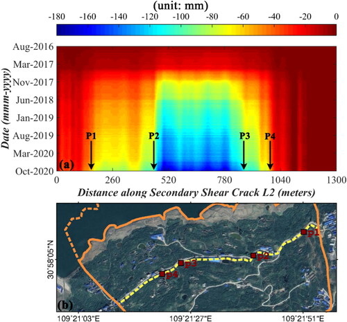
The spatially complete time-series deformation field provides vital information for locating the regions with severe damage. The LOS cumulative deformations are derived along the secondary shear outlet L2 (Figure 8(a)). It can be observed that the maximum LOS cumulative had achieved near 180 mm during the observation period of more than 4 years. The deformations are concentrated on the P1–P4 sections. In particular, the P2–P3 sections show significant ground movements. As shown in Figure 8(b), there are several buildings in the P2–P3 sections. The areas with the difference of deformation led to severe cracks. According to the in situ investigation, many cracks were found in the buildings in P2 and P3 (Figure S1(b,c)). Once the movement of the landslide accelerated, the buildings between P2 and P3 will suffer severe damage and life will be threatened. Therefore, it is necessary to clear the triggers and failure mode of the Xinpu landslide complex and adopt suitable measures for reducing risks.

Figure 8. (a) Cumulative deformations along the secondary shear outlet. (b) Corresponding location of the section with strong deformation. The background is a Google Earth image.

4.2. Triggers and lag time of the XET slope in different sections

IC4 and IC5 exhibit the most prominent signals within the XET slope and have been identified as independent components associated with landslide movements, as detailed in Text S1 and Figure S2. Figure 9(a,b) show the contributions of IC4 and IC5 after ICA postprocessing. It can be found that the deformations of the center and the toe of the XET slope show various spatial patterns, which indicate that they have distinct mechanisms. Most contribution of IC4 concentrates in the center section of the XET slope, which represents the deformation behind the secondary shear outlet. Figure 9(c) presents the relationships between the normalized eigenvectors of IC4, precipitation, and reservoir water level. It can be found that the time series of IC4 and water level are unrelated. The water level fluctuates every year, but there was no obvious fluctuation in IC4’s time series from 2018 to 2020. However, a significant consistency between cumulative precipitation and the normalized eigenvectors of IC4 can be observed (Figure 9(c), the green and red points). From 2018 to early 2020, there was no significant increase in cumulative precipitation in the Xinpu landslide complex, and the IC4’s time series showed a slow upward trend. Heavy precipitation happened in 2017 with a cumulant of 1,307 mm from April to October, and the time series of IC4 also greatly increased in this period, which corresponds to the significant movements in 2017 (Figure 7). The cross-correlation analysis between IC4 and cumulative precipitation was implemented, and a positive correlation of 0.99 between them was observed. Therefore, precipitation is suggested to be the main trigger of the strong deformation in the center section of the XET slope. This also accords with previous studies, which showed that precipitation usually drives an accelerated slip in the TGR area (Wang et al. 2004, 2019). Because of the infiltration of rainwater, the elevated pore-water pressure should be a reason for the instability in the XET slope (Hu et al. 2019).

Figure 9. Contribution of (a) IC4 and (b) IC5 derived by ICA. Comparisons between precipitation (green triangle), water level (blue areas), and normalized IC eigenvectors of (c) IC4 and (d) IC5. (e) & (f) Relationship between correlation and lag time for corresponding triggers.

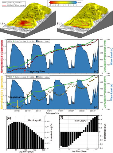
The toe evolution plays a critical role in the stability of slow-moving landslides (Ferrari et al. 2011; Wasowski and Pisano 2019). Owing to the derived spatially complete deformation field, the spatial–temporal pattern of the toe can be observed. The contribution of IC5 is distributed at the toe of the XET slope. The corresponding eigenvectors were adopted to compare with the reservoir water level and cumulative precipitation (Figure 9(d)). The time series of IC5 presents an obvious periodic law with a cycle of ∼1 year, which matches the fluctuation of the reservoir water level. Figure 9(d) exhibits that the normalized eigenvectors of IC5 increase during the discharge cycle. Similarly, when the water level is raised, a short decrease can be observed in IC5’s time series. The periodic fluctuation of the reservoir water level usually induces a stable–active cycle of landslide deformation in the TGR area (e.g. the Shuping landslide (Shi et al. 2015) and the Muyubao landslide (Shi et al. 2015)). For the landslides within the reservoir bank, the pressure difference is regarded as the reason for such a phenomenon (Paronuzzi et al. 2013; Shi et al. 2015). Specifically, during the impoundment period, the water pressure outside the landslide is higher than that in the interior. The inward pressure difference will cause the landslide in a stable state. While the water level declines because of the discharge operations, outward water pressure is produced, which will destabilize the bank slope and induce the increase of deformation (Figure 9(d)) (Paronuzzi et al. 2013). Cross-correlation analysis between the water level and IC5 was conducted, and a negative correlation was observed. However, the correlation only reached 0.31, which means that the reservoir water level may not be the only trigger of the toe of the XET slope.

Lag time is a critical parameter for understanding the landslides’ mechanism. Figure 9(c) shows that there is a lag time between cumulative precipitation and the time series of IC4. To estimate the lag time, the cross-correlation analysis between cumulative precipitation and IC4’s time series was implemented with different lag times. Figure 9(e) illustrates that the correlation reaches the peak with a lag of 45 days, which means that the movement will be initiated after intense rainfall 45 days later. This value is similar to most landslides, which are only affected by precipitation (for example, the Blakemont landslide in California (Cohen-Waeber et al. 2018) and the landslides in Wudu District (Liu et al. 2021)). The lag time also explains why accelerated movement lasts for about a month after the wet season.

The stability of the toe usually affects the total stability of the landslide (Ferrari et al. 2011; Wasowski and Pisano 2019). Cross-correlation analysis was employed to retrieve the lag time between IC5’s time series and the reservoir water level. It shows that the cross-correlation reaches the maximum when the lag time arrives at 21 days (Figure 9(f)), which is faster than that of IC4’s eigenvectors in response to cumulative precipitation. In addition, a difference in triggering times between the eigenvectors of IC4 and IC5 can be found; the deformation in the toe of the XET slope initiates earlier than that in the center (Figure 9(c,d), the red arrow). The predischarge of the Three Gorges Dam is inferred as a reason to induce such a difference in initiation times, which usually discharges the reservoir water before the intense rainfalls of the wet season.

5. Discussion

5.1. Performance of the proposed method

In this study, we utilize the proposed method to derive spatially complete time-series deformation, and good performance is shown in the derived results (Figure 5 and Figure 7). There are four main steps in the proposed method, in particular, the model-free inversion and ICA optimization play critical roles. Here, quantitative comparisons are implemented to indicate the effects in improving performance.

5.1.1. Effect of model-free inversion in improving the performance

Landslide movement is generally nonlinear in nature (Wasowski and Bovenga 2014). In the implemented method, we utilize the model-free inversion to derive the time-series deformation. Then, the nonparametric algorithm by the ICA method is utilized to optimize the derived time series, which can avoid the bias induced by the deformation model. Previous studies chose to obtain the time-series deformation with several deformation models and implement the spatial–temporal filter to optimize the residuals after removing the modeling deformation (e.g. (Berardino et al. 2002), (Zhang et al. 2011), and (Bateson et al. 2015)). The unsuitable filter window and abrupt deformation could lead to bias in the time-series deformation. To quantify the effects of the model-free inversion, we generate synthetic datasets and then derive the time series deformation with various methods. The synthetic data is divided into two parts (as shown in Figure 10 and Figure S3), area I is only affected by the linear deformation, as for area II, the periodic and abrupt signals are combined to generate the deformation (Figure 10(a)). Besides, the decorrelation noise and atmospheric effects are also added into the synthetic datasets.

Figure 10. Results of synthetic datasets. (a) Simulation deformation rate. (b-e) Deformation rates derived by conventional SBAS, ISBAS, and our method, respectively. (f-i) Residuals of the corresponding methods in the second row.

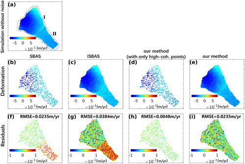
The derived results show that the linear deformation can be well estimated by each method. However, the non-linear deformation leads to the underestimation in the deformation derived by SBAS (Berardino et al. 2002) and ISBAS (Bateson et al. 2015) methods (Figure 10(b,c)), so significant biases can be observed in the residuals (Figure 10(f,g)). With the proposed method, the model-free inversion is utilized to derive the deformation, and the derived results illustrate the good performance on avoiding the bias caused by non-linear deformation (Figure 10(d,e,h,i)). For the time series deformation, a similar underestimation can be observed in the results derived by ISBAS (Figure S3). It should be noted that the intermittent points help increase the MPs, but the low coherence points will reduce the accuracy of the results (Figure 10(h,i)). When the results are derived from the high coherence points, our method can show better performance than the SBAS method (Figure 10(f,h)). A quantitative comparison is conducted by deriving the RMSE, the RMSE of ISBAS is 0.0384 m/yr, and the RMSE reaches 0.0235 m/yr from our method, an improvement of about 39% is achieved.

The proposed method can effectively alleviate the bias by utilizing the model-free inversion. Furthermore, we derived the initial time series by the arc and outlier detector to avoid phase ambiguity, which had been adopted in the TCP-InSAR method (Zhang et al. 2011). However, the difference is that the deformation model is replaced by the model-free inversion, which is beneficial for reducing significant residuals during the outlier detector process and retaining more MPs.

5.1.2. Effect of ICA in improving the performance

Although the model-free inversion can eliminate the bias, there are several errors (e.g. residual topography or atmospheric effects) in the initial time series. Hence, the ICA approach is utilized to optimize the initial time series. Since the end of 2019, six GNSS stations were built in the Xinpu landslide complex (as shown in Figure 1), here, G2-G5 monitoring results were adopted to evaluate the effect of ICA in improving the performance. Considering that the SBAS and distributed scatterers-based InSAR (DSI) (Ferretti et al. 2011) are both common approaches to deriving the spatial–temporal patterns of a slow-moving landslide, the results derived by these methods are also utilized for comparison.

Figure 11(a) presents that the spatial patterns derived by the classical SBAS method are sparse and most of the deformation areas cannot be detected. The main reason for the loss of MPs can be associated to seasonal variable vegetation, as inferred from the optical imagery (as shown in the background of Figure 11(a)). The long-sequence interferograms make it difficult for the MPs to maintain high coherence during the whole observation period; just the areas with steady surface features (e.g. house and road) can be detected, while the areas with seasonal variation vegetation will be lost in the annual LOS displacement field. DSI is a common approach that can improve the number of MPs. To obtain enough MPs, we also set 0.2 as the threshold of coherence to select the DS points. The result was improved after implementing the DSI method (Figure 11(b)). This illustrates that several areas can be covered by the denser MPs and that the deformation pattern can be observed. However, the main deformation area of the XET slope was still unavailable. After implementing the proposed method, the lost MPs are detected (Figure 11(c,d)). Clear spatial patterns are observed in the whole of the Xinpu landslide complex, which provided key information for understanding the mechanism of landslide. Besides, we find that the deformation rate after ICA optimization is larger than that without ICA optimization. To quantitate the differences between the results, the time-series deformation derived using distinct methods was implemented against in situ GNSS measurements.

Figure 11. Annual rate of movements derived using different MT-InSAR techniques in the Xinpu landslide complex. (a) SBAS, (b) DSI, (c) our method before ICA optimization, and (d) our method after ICA optimization. The background image used is a Google Earth image.

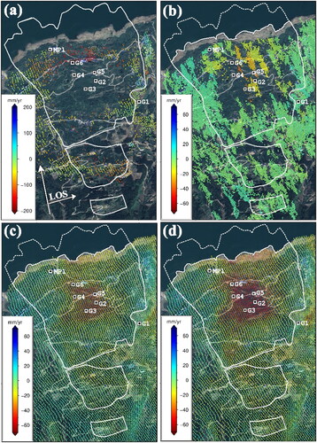
Because of the seasonal variation vegetation, as shown in Figure 11(a), the SBAS method cannot obtain any MPs in the GNSS monitoring stations. The comparison was implemented between DSI (only three MPs can be detected, e.g. G2, G3, and G5) and our method, and quantitatively evaluated against in situ GNSS measurements. Considering that the derived results are the projection of the actual movement, the three-dimensional (3D) GNSS measurements were converted to the Sentinel-1 LOS direction for comparison (Hu et al. 2014). For comparison, the accumulative time-series displacement of GNSS measurements is calibrated to corresponding Sentinel-1 observations at the end of 2019. The calibrated time-series results for all the GNSS stations are shown in Figure 12 (the green asterisk), with the corresponding root mean square (RMS). Prior to ICA optimization, the RMS values at G2 to G6 were 28.6, 32.3, 14.8, 19.9, and 13.3 mm, respectively. Subsequently, following ICA optimization, these RMS values at G2 to G6 exhibited improvements, measuring 12.7, 19.2, 6.9, 11.9, and 7.7 mm, respectively (as shown in Figure 12). Overall, time-series results derived using the proposed method matched well with those obtained using GNSS and represented similar trends at most GNSS stations.

Figure 12. Landslide time-series deformation derived by DSI (orange square), our method (before and after ICA optimization, shown with blue inverted triangle and red triangle, respectively), and GNSS observations (green asterisk) in (a) G2 (b) G3, (c) G4, (d) G5, and (e) G6 GNSS monitoring stations. The gray areas indicate the wet season of each year. (f) The time-series movements derived by various MT-InSAR methods.

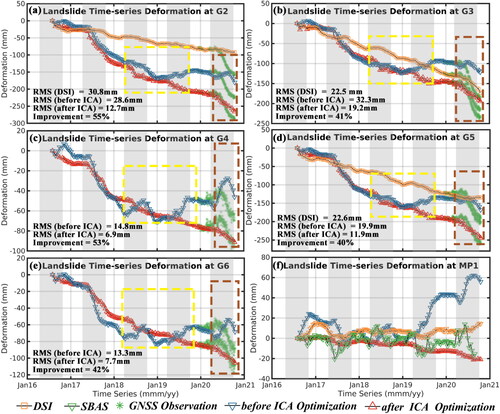
Before ICA optimization, all the GNSS stations exhibit discrepancies larger than 10 mm in the RMS between the GNSS and our method–derived results. It can be observed that the curve of the time-series deformation shows strong fluctuations (Figure 12, the yellow dashed boxes). Considering that the fluctuations are mainly distributed in the summer, it can be inferred that the APS phase and decorrelation noise could be the major factors affecting the derived time-series deformation. The DSI-derived time series can reduce significant fluctuations and retrieve a stable time series (Figure 12, the orange square). However, because of the low coherence, the accelerated deformation cannot be detected through the DSI-derived results, and it also leads to poor RMS. While it is possible to detect the accelerated signal by employing a higher-order polynomial to model deformation, this approach presents another challenge in that it may inadvertently incorporate a portion of the atmospheric phase into the deformation. After ICA optimization, the time-series deformation derived by our method is more stable. Besides, with the ICA optimization, the accelerated signals can be obtained in the proposed method–derived results (Figure 12, the brown dashed boxes), which are vital for landslide early warning. It can also be observed that the time-series deformation estimated by ICA optimization is closer to that derived by GNSS, wherein the accelerated signal is almost simultaneously detected by our method and GNSS measurements (Figure 12, the brown dashed boxes). We calculated the RMS between InSAR and GNSS. All the RMS values derived by ICA optimization are smaller than those derived without ICA optimization and DSI. Comparing the time series without ICA optimization, the average improvement achieves 46.2%. Therefore, this proves that the proposed method is able to overcome the APS phase and decorrelation noise to derive a reliable landslide time-series deformation for understanding the process of landslide movement.

However, significant discrepancies can be found at the G3 station. After ICA optimization, the RMS reaches 19.2 mm. The difference between InSAR and GNSS measurements could be attributed to several reasons. A spatial mismatch between the InSAR MPs and the GNSS stations could have been one of the factors. Because heterogeneous displacements were observed over the Xinpu landslide complex, as shown in Figure 11, a distance of tens of meters could induce obvious discrepancies in displacement measurements. Besides, because of the complex environment and installation technology, the GNSS measurement could also be the source of the discrepancies.

Seasonal deformations are among the most prevalent indicators of landslide activity. As previously outlined in Section 4, we have successfully identified substantial seasonal deformations within the Xinpu landslide region. At the toe of the slope, these deformations are associated with fluctuations in reservoir water levels, while within the primary landslide area, they correlate with rainfall patterns. To assess the effectiveness of various MT-InSAR monitoring techniques in capturing seasonal deformations, we designated a MP at the slope’s toe and conducted a comparative analysis of results using four different methods. Regrettably, the SBAS method could not obtain MPs in the region exhibiting the most pronounced seasonal movement at the slope’s toe, resulting in our acquisition of a common monitoring point, MP1, located beneath the primary landslide area, as illustrated in Figure 11. Analysis of the time-series deformations obtained from all methods at this point, as depicted in Figure 12(f), reveals that all methods can effectively monitor seasonal movements in the Xinpu landslide area. However, the SBAS method detected noteworthy fluctuations in its time-series deformations (Figure 12(f), indicated by green inverted triangles), which appear to be random in the temporal domain. Consequently, we attribute these fluctuations to a lower coherence threshold applied during SBAS MP selection. These fluctuations significantly impede the identification of seasonal deformation signals. In contrast, the DSI method produced time-series deformations with greater stability compared to the SBAS results (Figure 12(f), indicated by orange inverted triangles), successfully suppressing pronounced temporal signal fluctuations while revealing substantial periodicity. Nevertheless, this periodicity did not align with expected seasonality patterns. For instance, periodic signals exhibited a significant decline during the dry season in January 2017 and a notable increase during the wet season in June 2019, deviating considerably from the typical temporal behavior of landslides in the Three Gorges Reservoir area. We attribute this phenomenon to atmospheric phase effects. When utilizing the methodology proposed in this study, the time-series movements displayed analogous behaviors before the ICA optimization stage, including subsidence during the dry season of 2017 and substantial uplift during the wet season of 2019. As the phase prior to ICA optimization encompasses both atmospheric and deformation phases, we surmise that atmospheric influences primarily contribute to the observed signal. Post-ICA optimization, the time-series movements of landslides significantly improved. Atmospheric effects on temporal deformations were greatly attenuated, allowing for clear observation of landslide displacements induced by annual summer rainfall and changes in water levels. This underscores the capability of the method proposed in this study to reliably detect seasonal deformation signals associated with landslides.

Nevertheless, the aforementioned advantages of the implemented method depend on the high spatial–temporal resolution observations, which is also one of the limitations of the ICA algorithm. Hence, we utilized the intermittent points to increase spatial observation. A previous study has proven that nonlinear kinematics can be observed using the high sampling frequency of SAR data (Wasowski and Bovenga 2015). Owing to the large number of fast-revisited Sentinel-1 archives, nonlinear motion can be recognized in this study. However, because of the insufficient archive and lower revisiting period, our method cannot be robust in situations when early SAR data (e.g. ENVISAT ASAR and ALOS PALSAR) are exploited to investigate the history of the landslide movement. A possible solution is to combine multiplatform SAR data using the Multidimensional SBAS (MSBAS) (Samsonov et al. 2020) or Kalman Filter-based (KF) method (Hu et al. 2013) method so that the temporal solution can be increased to retrieve the nonlinear kinematics.

5.2. Joint effects of multiple triggers

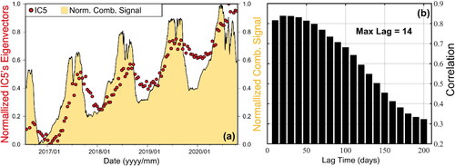
In addition to the periodic patterns, the eigenvectors of IC5 also present an increasing trend and show a positive correlation to the cumulative precipitation. Although the water level has been proven to be the main trigger of several landslides during the initial stage of the TGR (Tomás et al. 2014; Shi et al. 2015), precipitation is also observed to lead to the accelerated movement of the toe (Wasowski et al. 2017). The joint effects of precipitation and water level are, therefore, reasonable to be considered in the long-term observations. Because the cross-correlation between IC5 and water level is negative, the opposite of the reservoir water level and cumulative precipitation were normalized and combined to compare with IC5’s time series (Figure 13(a), the yellow areas). Figure 13(a) shows that the normalized combined signal is more consistent with the eigenvectors of IC5 than the normalized water level signal. The cross-correlation between the combined signal and periodic deformation reached 0.80, which is better than that between IC5’s time series and reservoir water level. This substantiates that the periodic fluctuation of the reservoir water level and cumulative precipitation are both triggers that affect the stability of the toe of the XET slope. The stability of the toe decreases as a result of groundwater fluctuation (Ferrari et al. 2011). In addition to the water level, the frequent rainfall also increases the groundwater and destabilizes the toe of the XET slope. Considering that the toe of the XET slope is affected by the joint effects of cumulative precipitation and reservoir water level, we implemented a cross-correlation analysis between the eigenvectors of IC5 and the combined signals with different lag times. The cross-correlation between the combined signal and periodic deformation reaches the peaks at a lag time of 14 days with a correlation of 0.85 (Figure 13(b)). This value is similar to the results observed in the Huangtupo landslide of the TGR (Tomás et al. 2014). Because precipitation can also change the water pressure difference (Ferrari et al. 2011), cumulative precipitation should be accounted for as the main reason for the decline in the lag time. During the discharge period, the reservoir water level will be decreased and water pressure outside the landslide will be smaller than that inside, forming an outward pressure difference (Shi et al. 2015). In the wet season, the discharged operation always couples with intense rainfall. Following the seepage, the intense rainfall increases the groundwater level inside the landslide, which not only enlarges the shear stress but also increases the outward water pressure difference. The larger outward water pressure difference will increase the magnitude of deformation and reduce the response time as observed in Figure 13(a).

Figure 13. (a) Comparison between IC5 (red dot) and the normalized combined signal (yellow areas) after combining the precipitation and water level records. (b) Relationship between correlation and lag time.

5.3. Kinematic process of the Xinpu landslide complex

With the information about triggers and corresponding lag time, the kinematic process of the Xinpu landslide complex can be inferred. To sum up, the process of the Xinpu landslide complex’s movement is affected by precipitation and fluctuation of the reservoir water level. Specifically, during the dry season, the TGR area is under an impoundment period, and the inward water pressure difference stabilizes the landslide. When the wet season comes, the discharge operation is initiated, and the stability of the toe of the XET slope is decreased and begins to creep. If the discharged operation is coupled with heavy precipitation, the stability in the toe of the XET slope will be further weakened and a more obvious deformation will be induced. Because of the secondary shear outlet, the center of the XET slope is only affected by the cumulative precipitation, and its response time to the trigger is larger than that of the toe. After intense rainfall for 45 days, obvious movements will be initiated. Even if the precipitation stops, the accelerated movement will also continue for about 45 days. Given the presence of a retaining wall along the secondary shear outlet, it is imperative to underscore the significance of monitoring the evolution of this secondary shear outlet and its associated retaining wall. Any compromise in the stability of the retaining wall poses a potential risk of causing substantial damage.

6. Conclusions

A framework is proposed for investigating the kinematics and triggers. This framework includes two parts, namely, the ICA-assisted intermittent MT-InSAR process and triggers and lag time estimation. The ICA-assisted intermittent MT-InSAR method is developed for achieving spatially complete time-series deformation in an area with seasonal variable vegetation. To this end, intermittent points, model-free inversion, and ICA optimization are utilized. An obvious advantage of the implemented method is that it does not need any prior model, which is usually required for estimating the time-series deformation, and can suppress the effects of APS and the decorrelation noise. The obtained results were compared and validated with the results obtained using other classical MT-InSAR methods and in situ GNSS observations, indicating that the density of MPs can be significantly improved and the average RMS can reach a near-millimeter level.

The spatially complete time-series deformation of the Xinpu landslide complex provides unique information for understanding the process of movement during the impoundment and discharge cycle of TGR. First, we derived the distribution and temporal behavior of deformation in the Xinpu landslide complex. We found that the area with strong deformation was distributed in the center and the toe of the XET slope. Secondary shear outlets affected the distribution of deformation, which blocks the deformation to extend from the center to the toe of the landslide. Second, we found that there were various triggers in different portions of the Xinpu landslide complex. The deformation showed a strong correlation with the cumulative precipitation at the center section of the XET slope, which may be a reason for the accelerated induced deformation during the summer of 2017 and 2020. The toe of the Xinpu landslide complex was affected by the joint effects of cumulative precipitation and the periodic reservoir water level. Third, we estimated the lag time of various triggers in different portions of the Xinpu landslide complex. The lag time of cumulative precipitation was 45 days in the center section of the XET slope, while that of the periodic reservoir water level was 21 days at the toe of the XET slope. The reservoir water level that accompanied the intense rainfall increased the outward water pressure difference toward the toe of the XET slope, which not only induced more severe deformation but also decreased the response time from 21 to 14 days. By jointly considering the spatial–temporal patterns, various triggers, and corresponding lag time, the process of movement in the Xinpu landslide complex was analyzed in this study.

This study demonstrated that the spatially complete deformation field can be derived in an area with seasonal variable vegetation during a long-term observation window. The spatially complete time-series deformation allowed us to track the history of landslides and enhance our understanding of landslide mechanisms. Nevertheless, deriving the spatial–temporal pattern with only LOS deformation may bring a few uncertainties to the results. Complete 3D surface deformations should be estimated for the Xinpu landslide complex in the future by joint analysis of multisource SAR datasets.

Acknowledgments

The authors would like to thank the European Space Agency (ESA) for providing the Sentinel-1 data.

Disclosure statement

No potential conflict of interest was reported by the authors.

Data availability statement

The Sentinel-1 data were provided by ESA/Copernicus (https://scihub.copernicus.eu/). Other datasets used to support the findings of this study are available from the corresponding author upon request.

Additional information

Funding

This study was supported by the National Natural Science Foundation of China (No. 42030112), the Nature Science Foundation of Hunan Province (Nos. 2022JJ30031, 2020JJ2043), the National Key Basic Research and Development Program of China (No. 2018YFC1505101), the Project of Innovation-driven Plan of Central South University (No. 2019CX007), and the Fundamental Research Funds for the Central Universities of Central South University (No. 2019zzts298).

References

- Bateson L, Cigna F, Boon D, Sowter A. 2015. The application of the intermittent SBAS (ISBAS) InSAR method to the South Wales Coalfield, UK. Int J Appl Earth Obs Geoinf. 34:249–257. doi:10.1016/j.jag.2014.08.018.
- Bayer B, Simoni A, Schmidt D, Bertello L. 2017. Using advanced InSAR techniques to monitor landslide deformations induced by tunneling in the Northern Apennines, Italy. Eng Geol. 226:20–32. doi:10.1016/j.enggeo.2017.03.026.
- Berardino P, Fornaro G, Lanari R, Sansosti E. 2002. A new algorithm for surface deformation monitoring based on small baseline differential SAR interferograms. IEEE Trans Geosci Remote Sensing. 40(11):2375–2383. doi:10.1109/TGRS.2002.803792.
- Cohen-Waeber J, Bürgmann R, Chaussard E, Giannico C, Ferretti A. 2018. Spatiotemporal patterns of precipitation-modulated landslide deformation from independent component analysis of InSAR time series. Geophys Res Lett. 45(4):1878–1887. doi:10.1002/2017GL075950.
- Colesanti C, Wasowski J. 2006. Investigating landslides with space-borne Synthetic Aperture Radar (SAR) interferometry. Eng Geol. 88(3–4):173–199. doi:10.1016/j.enggeo.2006.09.013.
- Comon P. 1994. Independent component analysis, a new concept? Signal Process. 36(3):287–314. doi:10.1016/0165-1684(94)90029-9.
- Ebmeier S. 2016. Application of independent component analysis to multitemporal InSAR data with volcanic case studies. JGR Solid Earth. 121(12):8970–8986. doi:10.1002/2016JB013765.
- Ferrari A, Ledesma A, González DA, Corominas J. 2011. Effects of the foot evolution on the behaviour of slow-moving landslides. Eng Geol. 117(3-4):217–228. doi:10.1016/j.enggeo.2010.11.001.
- Ferretti A, Fumagalli A, Novali F, Prati C, Rocca F, Rucci A. 2011. A new algorithm for processing interferometric data-stacks: squeeSAR. IEEE Trans Geosci Remote Sens. 49(9):3460–3470. doi:10.1109/TGRS.2011.2124465.
- Hu J, Ding X-L, Li Z-W, Zhu J-J, Sun Q, Zhang L. 2013. Kalman-filter-based approach for multisensor, multitrack, and multitemporal InSAR. IEEE Trans Geosci Remote Sens. 51(7):4226–4239. doi:10.1109/TGRS.2012.2227759.
- Hu J, Li Z, Ding X, Zhu J, Zhang L, Sun Q. 2014. Resolving three-dimensional surface displacements from InSAR measurements: a review. Earth Sci Rev. 133:1–17. doi:10.1016/j.earscirev.2014.02.005.
- Hu X, Bürgmann R, Lu Z, Handwerger AL, Wang T, Miao R. 2019. Mobility, thickness, and hydraulic diffusivity of the slow‐moving Monroe landslide in California revealed by L‐band satellite radar interferometry. JGR Solid Earth. 124(7):7504–7518. doi:10.1029/2019JB017560.
- Hu X, Burgmann R, Schulz WH, Fielding EJ. 2020. Four-dimensional surface motions of the Slumgullion landslide and quantification of hydrometeorological forcing. Nat Commun. 11(1):2792. doi:10.1038/s41467-020-16617-7.
- Huang B, Yin Y, Liu G, Wang S, Chen X, Huo Z. 2012. Analysis of waves generated by Gongjiafang landslide in Wu Gorge, three Gorges reservoir, on November 23, 2008. Landslides. 9(3):395–405. doi:10.1007/s10346-012-0331-y.
- Hyvärinen A, Oja E. 1997. A fast fixed-point algorithm for independent component analysis. Neural Comput. 9(7):1483–1492. doi:10.1162/neco.1997.9.7.1483.
- Hyvärinen A, Oja E. 2000. Independent component analysis: algorithms and applications. Neural Netw. 13(4-5):411–430. doi:10.1016/s0893-6080(00)00026-5.
- Hyvarinen A. 1999. Fast and robust fixed-point algorithms for independent component analysis. IEEE Trans Neural Netw. 10(3):626–634. doi:10.1109/72.761722.
- Intrieri E, Raspini F, Fumagalli A, Lu P, Del Conte S, Farina P, Allievi J, Ferretti A, Casagli N. 2017. The Maoxian landslide as seen from space: detecting precursors of failure with Sentinel-1 data. Landslides. 15(1):123–133. doi:10.1007/s10346-017-0915-7.
- Jiang H, Li Y, Zhou C, Hong H, Glade T, Yin K. 2020. Landslide displacement prediction combining LSTM and SVR algorithms: a case study of Shengjibao landslide from the three gorges reservoir area. Applied Sciences. 10(21):7830. doi:10.3390/app10217830.
- Karimzadeh S, Matsuoka M, Ogushi F. 2018. Spatiotemporal deformation patterns of the Lake Urmia Causeway as characterized by multisensor InSAR analysis. Sci Rep. 8(1):5357. doi:10.1038/s41598-018-23650-6.
- Li C, Fu Z, Wang Y, Tang H, Yan J, Gong W, Yao W, Criss RE. 2019. Susceptibility of reservoir-induced landslides and strategies for increasing the slope stability in the Three Gorges Reservoir Area: zigui Basin as an example. Eng Geol. 261:105279. doi:10.1016/j.enggeo.2019.105279.
- Li L, Yao X, Yao J, Zhou Z, Feng X, Liu X. 2019. Analysis of deformation characteristics for a reservoir landslide before and after impoundment by multiple D-InSAR observations at Jinshajiang River, China. Nat Hazards. 98(2):719–733. doi:10.1007/s11069-019-03726-w.
- Li S, Xu Q, Tang M, Iqbal J, Liu J, Zhu X, Liu F, Zhu D. 2018. Characterizing the spatial distribution and fundamental controls of landslides in the three gorges reservoir area, China. Bull Eng Geol Environ. 78(6):4275–4290. doi:10.1007/s10064-018-1404-5.
- Liao M, Tang J, Wang T, Balz T, Zhang L. 2011. Landslide monitoring with high-resolution SAR data in the Three Gorges region. Sci China Earth Sci. 55(4):590–601. doi:10.1007/s11430-011-4259-1.
- Liu P, Li Z, Hoey T, Kincal C, Zhang J, Zeng Q, Muller J-P. 2013. Using advanced InSAR time series techniques to monitor landslide movements in Badong of the Three Gorges region, China. Int J Appl Earth Obs Geoinf. 21:253–264. doi:10.1016/j.jag.2011.10.010.
- Liu Y, Qiu H, Yang D, Liu Z, Ma S, Pei Y, Zhang J, Tang B. 2021. Deformation responses of landslides to seasonal rainfall based on InSAR and wavelet analysis. Landslides. 19(1):199–210. doi:10.1007/s10346-021-01785-4.
- Paronuzzi P, Rigo E, Bolla A. 2013. Influence of filling–drawdown cycles of the Vajont reservoir on Mt. Toc slope stability. Geomorphology. 191:75–93. doi:10.1016/j.geomorph.2013.03.004.
- Peng M, Lu Z, Zhao C, Motagh M, Bai L, Conway BD, Chen H. 2022. Mapping land subsidence and aquifer system properties of the Willcox Basin, Arizona, from InSAR observations and independent component analysis. Remote Sens Environ. 271:112894. doi:10.1016/j.rse.2022.112894.
- Petley D. 2012. Global patterns of loss of life from landslides. Geology. 40(10):927–930. doi:10.1130/G33217.1.
- Samsonov S, Dille A, Dewitte O, Kervyn F, d‘Oreye N. 2020. Satellite interferometry for mapping surface deformation time series in one, two and three dimensions: a new method illustrated on a slow-moving landslide. Eng Geol. 266:105471. doi:10.1016/j.enggeo.2019.105471.
- Seguí C, Rattez H, Veveakis M. 2020. On the stability of deep‐seated landslides. The cases of Vaiont (Italy) and shuping (Three Gorges Dam, China). JGR Earth Surface. 125(7):e2019JF005203. doi:10.1029/2019JF005203.
- Shi X, Liao M, Li M, Zhang L, Cunningham C. 2016. Wide-area landslide deformation mapping with multi-path ALOS PALSAR data stacks: a case study of three gorges area, China. Remote Sens. 8(2):136. doi:10.3390/rs8020136.
- Shi X, Zhang L, Balz T, Liao M. 2015. Landslide deformation monitoring using point-like target offset tracking with multi-mode high-resolution TerraSAR-X data. ISPRS J Photogramm Remote Sens. 105:128–140. doi:10.1016/j.isprsjprs.2015.03.017.
- Shi X, Zhang L, Tang M, Li M, Liao M. 2017. Investigating a reservoir bank slope displacement history with multi-frequency satellite SAR data. Landslides. 14(6):1961–1973. doi:10.1007/s10346-017-0846-3.
- Singleton A, Li Z, Hoey T, Muller JP. 2014. Evaluating sub-pixel offset techniques as an alternative to D-InSAR for monitoring episodic landslide movements in vegetated terrain. Remote Sens Environ. 147:133–144. doi:10.1016/j.rse.2014.03.003.
- Sousa JJ, Hooper AJ, Hanssen RF, Bastos LC, Ruiz AM. 2011. Persistent scatterer InSAR: A comparison of methodologies based on a model of temporal deformation vs. spatial correlation selection criteria. Remote Sens Environ. 115(10):2652–2663. doi:10.1016/j.rse.2011.05.021.
- Tomás R, Li Z, Liu P, Singleton A, Hoey T, Cheng X. 2014. Spatiotemporal characteristics of the Huangtupo landslide in the Three Gorges region (China) constrained by radar interferometry. Geophys J Int. 197(1):213–232. doi:10.1093/gji/ggu017.
- Tomás R, Li Z, Lopez-Sanchez JM, Liu P, Singleton A. 2015. Using wavelet tools to analyse seasonal variations from InSAR time-series data: a case study of the Huangtupo landslide. Landslides. 13(3):437–450. doi:10.1007/s10346-015-0589-y.
- Wang F-W, Zhang Y-M, Huo Z-T, Matsumoto T, Huang B-L. 2004. The July 14, 2003 Qianjiangping landslide, Three Gorges Reservoir, China. Landslides. 1(2):157–162. doi:10.1007/s10346-004-0020-6.
- Wang J, Ward SN, Xiao L. 2019. Tsunami Squares modelling of the 2015 June 24 Hongyanzi landslide generated river tsunami in Three Gorges Reservoir, China. Geophysical Journal International. 216(1):287–295. doi:10.1093/gji/ggy425.
- Wasowski J, Bovenga F, Nutricato R, Nitti DO, Chiaradia MT. 2017. Detection and Monitoring of Slow Landslides Using Sentinel-1 Multi-temporal Interferometry Products, 249–256.
- Wasowski J, Bovenga F. 2014. Investigating landslides and unstable slopes with satellite Multi Temporal Interferometry: current issues and future perspectives. Eng Geol. 174:103–138. doi:10.1016/j.enggeo.2014.03.003.
- Wasowski J, Bovenga F. 2015. Remote sensing of landslide motion with emphasis on satellite multitemporal interferometry applications, 345–403.
- Wasowski J, Pisano L. 2019. Long-term InSAR, borehole inclinometer, and rainfall records provide insight into the mechanism and activity patterns of an extremely slow urbanized landslide. Landslides. 17(2):445–457. doi:10.1007/s10346-019-01276-7.
- Xiong Z, Feng G, Feng Z, Miao L, Wang Y, Yang D, Luo S. 2020. Pre- and post-failure spatial-temporal deformation pattern of the Baige landslide retrieved from multiple radar and optical satellite images. Eng Geol. 279:105880. doi:10.1016/j.enggeo.2020.105880.
- Xu S, Niu R. 2018. Displacement prediction of Baijiabao landslide based on empirical mode decomposition and long short-term memory neural network in Three Gorges area, China. Computers & Geosciences. 111:87–96. doi:10.1016/j.cageo.2017.10.013.
- Ye X, Zhu H-H, Cheng G, Pei H-F, Shi B, Schenato L, Pasuto A. 2023. Thermo-hydro-poro-mechanical responses of a reservoir-induced landslide tracked by high-resolution fiber optic sensing nerves. J Rock Mech Geotech Eng. doi:10.1016/j.jrmge.2023.04.004.
- Ye X, Zhu HH, Wang J, Zhang Q, Shi B, Schenato L, Pasuto A. 2022. Subsurface multi‐physical monitoring of a reservoir landslide with the fiber‐optic nerve system. Geophys Res Lett. 49(11):e2022GL098211. doi:10.1029/2022GL098211.
- Zhang L, Ding X, Lu Z. 2011. Modeling PSInSAR time series without phase unwrapping. IEEE Trans Geosci Remote Sens. 49(1):547–556. doi:10.1109/TGRS.2010.2052625.
- Zhang L, Sun Q, Hu J. 2018. Potential of TCPInSAR in monitoring linear infrastructure with a small dataset of SAR images: Application of the Donghai Bridge, China. Appl Sci. 8(3):425. doi:10.3390/app8030425.
- Zhou C, Cao Y, Yin K, Wang Y, Shi X, Catani F, Ahmed B. 2020. Landslide characterization applying sentinel-1 images and InSAR technique: the Muyubao landslide in the three gorges reservoir Area, China. Remote Sens. 12(20):3385. doi:10.3390/rs12203385.