MMINP: A computational framework of microbe-metabolite interactions-based metabolic profiles predictor based on the O2-PLS algorithm

ABSTRACT

The gut metabolome acts as an intermediary between the gut microbiota and host, and has tremendous diagnostic and therapeutic potential. Several studies have utilized bioinformatic tools to predict metabolites based on the different aspects of the gut microbiome. Although these tools have contributed to a better understanding of the relationship between the gut microbiota and various diseases, most of them have focused on the impact of microbial genes on the metabolites and the relationship between microbial genes. In contrast, relatively little is known regarding the effect of metabolites on the microbial genes or the relationship between these metabolites. In this study, we constructed a computational framework of Microbe-Metabolite INteractions-based metabolic profiles Predictor (MMINP), based on the Two-Way Orthogonal Partial Least Squares (O2-PLS) algorithm to predict the metabolic profiles associated with gut microbiota. We demonstrated the predictive value of MMINP relative to that of similar methods. Additionally, we identified the features that would profoundly impact the prediction performance of data-driven methods (O2-PLS, MMINP, MelonnPan, and ENVIM), including the training sample size, host disease state, and the upstream data processing methods of the different technical platforms. We suggest that when using data-driven methods, similar host disease states and preprocessing methods, and a sufficient number of training samples are necessary to achieve accurate prediction.

KEY POINTS

• MMINP fully considers internal and mutual correlations in metabolites and microbial genes and infers metabolite information through their real joint parts.

• The feasibility of predicting metabolic profiles using gut microbiome data should be based on the premise of similar host disease states, similar preprocessing methods, and a sufficient number of training samples.

• Although the accuracy of predicted specific metabolites is affected by multiple factors, the systematic conclusions presented for predicted metabolites at higher levels (e.g., class level) are accurate, allowing metabolite prediction to be applied to the discovery of potential metabolite markers.

KEYWORDS:

• metagenome
• metabolome
• prediction
• data-driven method

Introduction

The gut microbiota is closely associated with human health and diseases.^1–3 It mainly functions by synthesizing, degrading, and modifying metabolites, which directly impact host development and physiology, through its functional genes.^4–6 Therefore, a greater understanding of microbial metabolites can elucidate the mechanisms underlying their biological effects.⁷ While the repertoire of large-scale cohort microbiome data is rapidly increasing and is publicly available,^8,9 the corresponding metabolites data is scarce. This relative lack of metabolite information limits their strength in inferring functions and important biological targets. Several bioinformatics tools have been developed in recent years to predict the metabolite profiles based on metagenomic data, which can help fill the gaps in metabolome data and encourage population-scale discovery of novel associations and biological targets without requiring costly metabolomic analysis.

The predictive tools for metabolites based on microbiome data can be broadly divided into two categories. The first category relies on prior knowledge of metabolic pathways that link microbial genes and compounds, such as stoichiometric enzyme reaction matrices derived from the Kyoto Encyclopedia of Genes and Genomes (KEGG) database.¹⁰ Examples include PRMT¹¹ and MIMOSA¹² which can predict microbial community-wide metabolite turnover. The predictive accuracy of these tools is highly reliant on the annotation of microbial genes and the availability of data on biochemical reactions. The second category includes data-driven methods such as MelonnPan¹³ and ENVIM,¹⁴ which can predict the abundance of metabolites by training models through elastic net regularized regression using paired microbiome and metabolites data. Since these strategies do not require prior knowledge of metabolic pathways, they can circumvent the limitations of reference-based methods as described above. Nevertheless, metabolic processes are carried out through a series of enzymatic reactions, and the abundance of metabolites or genes can be affected by a multitude of metabolites and genes. However, the current data-driven methods model each metabolite separately with genes.

Accordingly, we developed the MMINP (Microbe-Metabolite INteractions-based metabolic profiles Predictor) computational framework to predict microbial community-based metabolic profiles with the Two-Way Orthogonal Partial Least Squares (O2-PLS)^15,16 algorithm. O2-PLS, derived from the basic partial least squares projections to latent structure (PLS)¹⁷ prediction approach integrated with an integral orthogonal signal correction (OSC) filter,¹⁸ is a latent variable regression method. Compared to elastic network regression models, which deal with one dependent variable (metabolite) and multiple independent variables (microbial genes) each time, the O2-PLS algorithm considers the two data matrices (metabolites and microbes) equally such that it is predictive in both directions, and models all features simultaneously to extract joint components, specific components and residual components from both matrices. It separates structure noises,¹⁹ which are defined as systematic variations not linearly correlated with the other omics, from the joint covariation through OSC filter, and identifies the interaction of two omics’ real joint parts. Referred to the modeling approach from MelonnPan, which only retains “well-predicted metabolites” (WPMs), we defined “well-fitted metabolites” (WFMs) to improve prediction accuracy of our model (detailed in Methods). We assessed the prediction performance of MMINP and used the predicted values for downstream biological analyses. In addition, the performance of MMINP, MelonnPan, ENVIM, and O2-PLS were compared, and the impact of training sample size, host disease state and data processing methods (here referring to technical platforms and upstream data processing methods) on these methods were evaluated using our collected datasets. The implementation of MMINP is available at GitHub (https://github.com/YuLab-SMU/MMINP) and the Comprehensive R Archive Network (https://cran.r-project.org/package=MMINP).

Results

MMINP workflow

MMINP trains a model using samples with both microbiome and metabolome data before predicting the metabolites. Given that the taxonomic composition of microbiomes varies significantly across hosts while their community gene context is highly conserved,²⁰ MMINP uses the abundance of microbial genes rather than that of species to predict the metabolites.

The main procedures of MMINP are data preprocessing, model training, and prediction. During the data preprocessing stage, it is recommended that the extremely rare features with low abundance and prevalence in the microbiome and metabolome data (≤0.01% in ≥ 90% of samples) be eliminated. The relative abundance of the remaining features in both datasets is subjected to Box-Cox transformation and scaling to reduce deviations in magnitude.²¹ Prior to this, zero values are smoothed out using half the smallest non-zero measurement on a per-sample basis.²²

At the beginning of the training stage, an initial O2-PLS model is built after determining the component numbers using a standard or a faster alternative cross-validation method.²³ Since not every metabolite is primarily regulated by microbes,^24–26 the inclusion of these metabolites in the model may negatively impact its prediction performance. To ensure that the trained model can predict a larger number of metabolites with a higher degree of accuracy, we defined WFMs as those with a spearman correlation coefficient (predicted versus measured abundance in the training data) higher than a threshold (default to 0.4, Figure S1a–c, detailed in Methods). Briefly, the WFMs are selected from the metabolome data and re-modeled with the microbiome data, and the procedure is repeated until all retained metabolites in the new model are WFMs (Figure 1a). The final model can be applied to predict metabolites in analogous environments using new microbial feature data (Figure 1b). The predicted metabolites (PMs) of newly acquired microbial feature data by the model are identical to the WFMs in the final model.

Figure 1. MMINP workflow. (a) Training MMINP model with pre-processed metabolome (Y: metab(N,M)) and metagenome (X: metag(N,K)) data; N, the sample size of training data; M, the number of metabolites; K, the number of bacteria. step 1) construction of an O2-PLS model with preprocessed microbial genes (X) and metabolites (Y) data; step 2) prediction of metabolites using the model built in step 1; step 3) spearman correlation analysis between measured values and predicted values, metabolites with correlation coefficient greater than 0.4 would be defined as WFMs; step 4) the model will retrain until all the metabolites in the model are WFMs (remove metabolites except WFMs from Y and repeat step 1–3 until all retained metabolites are WFMs). (b) New metagenomes with overlapping genes (overlapping ratio more than ‘minGenesize’) with MMINP model can be predicted by the model. WFMs, well-fitted metabolites.

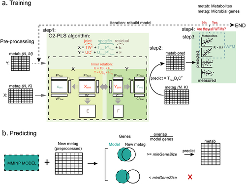
The prediction is made according to the prediction algorithm in O2-PLS. Genes that exist in the model but not in the new feature table are substituted with zero. This missing information would affect the prediction. Therefore, if the proportion of the overlapped genes between new microbial feature data and the model, relative to the total number of genes in the model, is less than “minGeneSize” (default to 0.5, Figure S1d, detailed in Methods, can be adjusted by the user), the prediction process will be terminated, and a novel model, trained on data that is analogous to the samples under consideration, will be required. To evaluate the predicted results of our model, we referred to Cohen’s criterion,²⁷ which considers a correlation coefficient of 0.3 to be a medium effect size. Therefore, metabolites with a spearman correlation coefficient (predicted versus measured metabolite abundance in the testing data) greater than 0.3 are defined as WPMs, similar to the procedure for MelonnPan.

MMINP predicted most metabolites accurately using microbial genes

We used the Inflammatory Bowel Disease (IBD) data sets (D1 in Supplementary File 1) to evaluate the prediction performance of MMINP since previous studies have demonstrated distinct metabolic profiles of IBD patients and healthy controls. The MMINP model was built using 155 discovery samples to predict the metabolite profiles of 65 samples in the validation cohort. The predicted values were compared to the measured metabolomic data of the validation cohort. After removing the rare features of the discovery samples, 2794 clustered metabolites and 1102 microbial genes were used for modeling. Approximately half of the metabolites (n = 1444) had been assigned to a putative chemical class.²²

Recommended by fivefold cross-validation, the MMINP model was built with six joint components, six genetic-specific components, and four metabolic-specific components. The variations in the genes and metabolites explained by the model were 60.7% and 55.3% respectively. Joint correlations could explain 44.3% of the total variations in genes and 41.5% of the total variations in metabolites. The genes explained 33.5% of metabolite variations, which comprised 80.7% of the explicable variations (41.5%) in the metabolites. MMINP finally obtained 2015 (72.1%) WFMs in the model, of which 1233 (61.2%) were WPMs in the validation data. Nearly half of these WPMs were previously unassigned (Figure 2a), which could also be a potential target for downstream analysis and characterization in future studies. Among 1444 previously annotated metabolites, dipeptides, long−chain fatty acids, amino acids, peptides, and analogues were the predominant classes. In addition, sphingolipids, tetrapyrroles, and organonitrogen compounds had the highest number of WPMs, and all alkyl−phenylketones, salicylic acids, quinolines and derivatives, and phenylbenzodioxanes were WPMs (Figure 2b and S2a).

Figure 2. The prediction performance of MMINP. (a) The predicted situation of metabolites. NIM (metabolites not in the model): the input metabolites which are removed during modeling. WPM (well-predicted metabolites): metabolites with a spearman correlation coefficient (predicted versus measured metabolites abundance in testing data) no less than 0.3. PPM (poorly predicted metabolites): metabolites with a spearman correlation coefficient less than 0.3. Assigned: metabolites assigned to putative chemical classes by comparing with the Human Metabolome Database. Unassigned: metabolites without assignment. WFMs (well-fitted metabolites), identical to predicted metabolites (PMs), is the sum of WPMs and PPMs. (b) Barplot of NIMs, PPMs, and WPMs of each putative chemical class. Classes with at least five well-predicted metabolites are displayed. (C) Procrustes analysis on metabolite profiles between predicted and measured values based on Eucildean distance (M² = 0.389, P = 0.001); each line links the predicted and measured features of one sample. Shorter bars (corresponding to a lower M²) indicate that a more similar relationship between the predicted and measured features of the sample. Blue points represent samples from control. Red points represent samples from CD. Yellow points represent samples from UC.

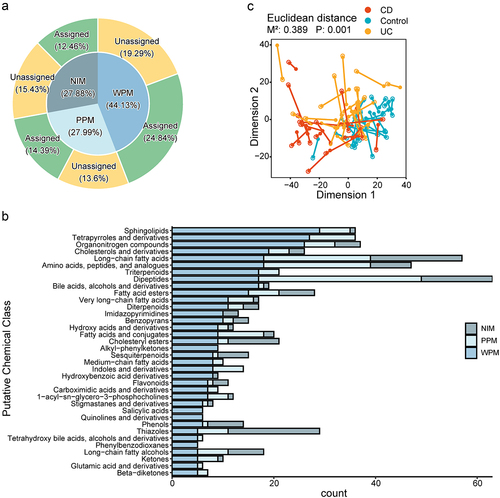
Procrustes analysis was applied to assess the similarity of metabolite profiles between measured and predicted methods. Compared to microbial gene abundances (M² = 0.79, P = 0.001), predicted metabolic profiles had higher similarity with true metabolites (M² = 0.389, P = 0.001), indicated by the smaller M² (Figure 2c and S2b).

In summary, these results demonstrated that MMINP could predict most metabolites accurately using microbial genes.

The biological significance of MMINP prediction

To determine whether MMINP prediction can uncover disease-related biological signatures, we tested the PMs in the validation cohort, which included 22 control samples, 23 ulcerative colitis (UC) patients, and 20 Crohn’s disease (CD) patients. As illustrated in Figure 3a and S3a, the predicted metabolite profile was able to differentiate between CD/UC and control samples, similar to the measured metabolites. We then evaluated the ability of MMINP to identify differentially abundant metabolites between CD/UC and control samples by comparing differentially abundant metabolites identified by prediction with those identified by measurement in number, variety, and variation tendency. There were 89.6% (817/912, CD vs. Control) and 50.3% (244/485, UC vs. Control) of differentially abundant metabolites that could be recurrence by predicted metabolites (Figure S3b,c). The shared differentially abundant metabolites between CD/UC and control samples identified by the predicted and measured values showed the same trend (Figure 3b and S3d,e). Nearly all differentially abundant sphingolipids and bile acids were increased in the CD group (Figure 3b) while the indoles (Figure S3d) were decreased, which is consistent with previous reports.²⁸ The distribution of the PMs assigned to the sphingolipids, bile acids, and indoles was similar to the distribution of their measured values (Figure S4).

Figure 3. The downstream analysis of MMINP prediction. (a) Comparison of metabolite profiles between CD and Control samples by principal component analysis (PCA) and permutational multivariate analysis of variance based on Euclidean distance matrices using measured (above) and predicted metabolome (below). (b) Boxplot of the median difference of differentially abundant metabolites between CD and control in each putative chemical class. Tested by Wilcoxon rank sum test with Benjamini-Hochberg correction for multiple comparisons (FDR <0.05). Classes with at least five well-predicted metabolites are presented. (c) Over-representation analysis (ORA) on chemical classes associated with the differentially abundant metabolites in each group.

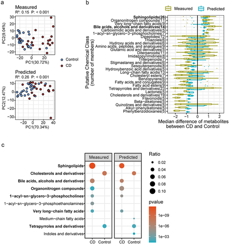
To interpret the result systematically and find clues to the explanation of the underlying mechanism, by over-representation analysis (ORA), we focused on discovering important chemical classes at the higher-order taxonomy level, in which most members were significantly changed. The significant classes that were enriched by differentially abundant metabolites identified through predicted values exhibited consistency with the enrichment outcomes of measured values (Figure 3c and S5), and most were related to lipid metabolism. In particular, the enrichment of sphingolipids, very long-chain fatty acids, and bile acids in the CD group, and that of cholesterols, tetrapyrroles, and indoles in the control group (Figure 3c) are consistent with previous findings.^{4, 28–31}

We next identified the potential driven enzymes and species associated with the significant metabolite classes. The differentially abundant genes involved in the KEGG pathways that correlated with the significant metabolite classes were screened, and their correlations with the differentially abundant species were analyzed in order to identify the key genes and species driving metabolite alterations. Glucosylceramidase, a key enzyme in sphingolipid metabolism that hydrolyzes glucosylceramide into glucose and ceramides, was decreased in CD samples (Figure S6a). This is consistent with a previous study showing that ceramide supplementation can alleviate the symptoms of IBD in a mouse model.³² Thus, the gene encoding this enzyme may be a key driver of the alterations in sphingolipids and derivatives observed during gut inflammation. Alistipes shahii can encode glucosylceramidase, and its lower abundance in CD patients may be the underlying cause of the low enzyme levels. However, we did not observe correlations between the abundance of every species and their specific genes (Figure S6), likely because many species share common genes and the differential expression levels of several genes were the result of changes in multiple bacteria. Furthermore, some species showed a negative correlation with their characteristic gene, such as Ruminococcus gnavus and prephenate dehydrogenase. Likewise, some species showed strong positive correlations with genes that have never been detected in the particular species, which can be attributed to the limitations of detection and analysis methods, or due to indirect correlation.

In summary, MMINP predictions can provide metabolomics information, identify biomarkers related to significant metabolite classes, and elucidate biological relationships when combined with metagenome data.

MMINP yielded the highest precision and F1 score

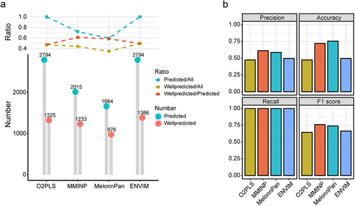
We compared the prediction performance of MMINP to that of MelonnPan (v0.99.0, 2021-02-08) and ENVIM using the training set and testing set described above. Given that the original O2-PLS model can be used to predict metabolites, we included it in our comparative analysis. By utilizing the number of PMs and WPMs, the ratio of PM/All, WPM/All, WPM/PM, precision, accuracy, and F1 score, we assessed the prediction performance of O2PLS, ENVIM, MMINP, and MelonnPan (Figure 4, Figure S7). In the O2-PLS model, genes explained 27.7% of the metabolite variations which was 78.9% of the explainable variations in metabolites (Supplementary File 2). MMINP and MelonnPan predict metabolites while trimming those with low predictive accuracy, whereas O2PLS and ENVIM retain all metabolites in the model. This difference in approach leads to a higher number of predicted metabolites of O2PLS and ENVIM. (Figure 4a). The WPMs for O2PLS, ENVIM, MMINP, and MelonnPan were 1325, 1386, 1233, and 976, respectively, with a majority of the WPMs being shared among four tools (Figure S8). MMINP had the highest ratio of WPM/PM among the four methods. MMINP and MelonnPan performed better in terms of precision, accuracy, and F1 score (Figure 4b).

Figure 4. The comparison of prediction performance among O2-PLS, MMINP, MelonnPan, and ENVIM. (a) the bottom part shows the number of PMs and WPMs, while the upper part shows the PM/All ratio, WPM/All ratio, and WPM/PM ratio. All: the input metabolites for modeling. Predicted: metabolites predicted by the model, i.e., metabolites in the model. Wellpredicted: metabolites with a spearman correlation coefficient (predicted versus measured metabolites abundance in testing data) greater than 0.3. (b) Barplot of Precision, Accuracy, Recall and F1 score among O2-PLS, MMINP, MelonnPan, and ENVIM.

The above comparison included unannotated metabolites, we next compared the prediction performance of the four methods for only features that had KEGG annotations. In addition, we also applied the four methods for the annotated features in two other datasets with paired gut microbiome and metabolome data (details in Supplementary File 1). For each dataset, two-thirds of the samples were used as the training set and the remaining samples as the testing set. Consistent with the results using the D1 dataset, MMINP yielded the highest WPM/PM ratio, precision, and F1 score, followed by MelonnPan, while O2-PLS and ENVIM obtained more PMs and WPMs (Supplementary File 2).

Impact of sample size, disease state, and data processing on the prediction performance

As a data-driven method, the prediction performance of MMINP, as well as the other three methods, would be affected by the training samples. Therefore, we analyzed the impact of training sample size, host disease state, and data processing methods on the performance of MMINP and the other models.

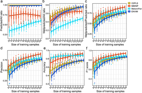
As shown in Figure 5, the proportion of PMs fluctuated in MMINP and increased consistently in MelonnPan with the increase in modeling sample size, while the WPM/PM ratio continuously increased for all methods and began to plateau when the sample size exceeded 50. Furthermore, the WPM/PM ratio, precision, and F1 score were highest for MMINP compared to the other methods. In Figure 5a,b, we did not observe the plateau in the curves representing MelonnPan, which indicated that MelonnPan required more training samples to achieve a higher proportion of predictable metabolites compared with the other three methods.

Figure 5. The impact of training sample size on the prediction performance. (a–f) the PM/All ratio (a), WPM/All ratio (b), WPM/PM ratio (c), Precision (d), Accuracy (e), and F1 score (f) of models constructed by training samples with different sizes when predicting metabolites of the test set.

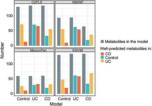
In terms of host disease states, we used samples from CD, UC, or control groups respectively to build a model and apply it to the samples of the other two groups. The model based on controls showed better predictive ability for the metabolites in UC compared to the CD samples, and the model based on CD samples performed better for UC than the control (Figure 6, Supplementary File 3). In contrast, the model based on UC samples showed similar prediction performance for the control and CD samples (Figure 6, Supplementary File 3). This is partly because of the fact that almost half of the UC patients have less distinct metabolite profiles compared to the non-IBD controls.²² Thus, the host disease state can affect the prediction.

Figure 6. The impact of host disease state on prediction performance. Samples from CD, UC, or control group were respectively used to build the model and apply it to the samples of the other two groups. Barplot shows the number of metabolites. Grey bars represent the number of well-fitted metabolites in each model. Red bars represent the number of well-predicted metabolites using each model to predict samples from CD. Blue bars represent the number of well-predicted metabolites using each model to predict samples from the control. Yellow bars represent the number of well-predicted metabolites using each model to predict samples from UC.

The number of WPMs decreased when data obtained from different platforms and preprocessed using different methods were used for modeling and predicting (Supplementary File 4). It may partly be due to differences in host disease states and the small number of shared features between models and testing sets. Therefore, we used only the shared features of control samples from the three datasets to rebuild models and predict each other. Only a few metabolites were WPMs (Supplementary File 5), suggesting that the prediction performance is impaired if the predicted and training data are obtained from different platforms and subjected to different preprocessing methods.

In summary, the feasibility of predicting metabolic profile with gut microbiome data should base on the premise of similar host disease states, similar processing methods, and a sufficient number of training samples (greater than 50).

Discussion

We developed MMINP based on the O2-PLS algorithm to predict metabolite abundance using microbial data. The O2-PLS algorithm can quantify data-specific variations and discover relationships between two omics data and has been mostly applied to omics data integration.³³ However, it involves a number of irrelevant variables that do not enhance the interpretability and predictability of the model.³⁴ The relevance of variables in the O2-PLS model is determined by calculating the variable influence on projection (VIP) values,³⁵ and those with VIP values less than 0.5 are excluded. However, the VIP values for all metabolites were close to each other in our O2-PLS model, and only a few had a VIP value over 0.5. On that basis, we defined “well-fitted metabolites” to distinguish important metabolites from the irrelevant variables, and only included them in the final model. Our findings indicate that MMINP can predict most metabolites accurately, and help identify potential disease-related biomarkers for experimental validation.

This tool has some limitations that must be considered. Firstly, although cross-validation functions are offered for choosing tuning parameters of a model while limiting the risk of overfitting, it is challenging to determine an appropriate number of components since a suitable number of folds and ranges of component numbers have to be selected previously based on subjective experience. One possible solution could be selecting a wide range of values at the cost of a larger expense of computing time. Secondly, MMINP provides estimates of the relative abundance of metabolites instead of directly predicting metabolite peaks. Nevertheless, a consistent pattern between the predicted and measured relative abundance of the metabolites is sufficient to inform subsequent experimental validation studies on metabolites of interest. Thirdly, we only applied MMINP on the human gut and untargeted MS-based metabolomics data, which needed further investigations in other microbial environments and assay types. Finally, since MMINP is based on a latent variable regression method, it would be unlikely to distinguish the original taxa of metabolites. However, the PMs can be analyzed in conjunction with other data to identify the bacteria and genes associated with key metabolites.

We also compared the prediction performance of MMINP with that of similar tools and the simple O2-PLS model. While O2-PLS and ENVIM retained all metabolites in the model, MMINP and MelonnPan only retained those that met the respective requirements. Therefore, while the first two methods predicted more metabolites, the latter two had a higher percentage of WPMs. In addition, MMINP showed the highest precision and F1 score among all methods. The choice between these methods is more of a subjective preference for the number of WPMs or the accuracy of predictions. However, while all four methods were able to capture a certain number of metabolites, it should be acknowledged that there is still a considerable gap in achieving high-quality predictions. Given that the gut metabolome is influenced by multiple variables, gut microbiota alone may have a limited role in determining metabolite levels. Therefore, the performance of both data-driven and knowledge-driven methods may be constrained by the complex relationship between gut metabolites and factors, including bacteria, environmental features, and diet, which necessitates further studies using more comprehensive data sources and advanced algorithms.

Since the technical platforms and upstream data processing methods influence metagenomic and metabolomic data, they may also impact the prediction performance of tools based on these data. The effect was illustrated by our results. Therefore, it is critical to choose a model that has been trained using the same technical platforms and processing methods as the data to be predicted. We also found that the prediction performance of MMINP improved significantly with the increase in training sample size, and slowly when the sample size was greater than 50. The metabolic capacity of microbes varies within the ecological environment,³⁶ and therefore relationships between microbes and metabolites may differ depending on some pathological changes, partly explaining the effect of the host disease state on prediction performance.

To construct an appropriate model and predict accurately, large amounts of modeling samples and prediction samples should be measured and preprocessed using the same procedures. While incorporating the maximum amount of data and including various situations to build a generalized model is ideal, it is practically not feasible. The best approach is to select representative samples (ideally no less than 50) to simultaneously measure metagenomic and metabolomic data, and then construct a model to predict the metabolites of the remaining samples based on their metagenomic data. Another possibility is to train the model with data that is associated with similar conditions as the data to be predicted. On the other hand, although the accuracy of predicting specific metabolites is affected by multiple factors, the systematic conclusions for these PMs at higher levels (e.g., class level) are accurate. Thus, we can identify changes in metabolic classes and screen for biomarkers associated with metabolic disorders or microbiome imbalance by predicting metabolites.

To summarize, MMINP can accurately predict metabolites using metagenomic data, which can be applied to discover potential biomarkers and elucidate disease mechanisms in the absence of metabolomics data. For achieving accurate prediction, we recommend employing similar host disease states and preprocessing methods, and a sufficient number of training samples when utilizing data-driven methods.

Methods

Description of the datasets

Datasets with paired gut microbiome and metabolome data were collected from three studies. All data had already been processed in the original studies, and tables of processed metabolite, microbial species and microbial gene abundance were available as their supplementary files with open access, or on public databases. More details are provided in Supplementary File 1 and Supplementary Methods.

Parameters in MMINP workflow

WFMs were defined as those with a spearman correlation coefficient (predicted versus measured abundance in the training data) higher than a pre-determined threshold. The WFMs in the final model are identical to the predicted metabolites of newly acquired microbial feature data by the model. To set the threshold of WFM, we randomly selected two-thirds of the original discovery samples from the IBD study²² (details in Supplementary Methods) as the training set, and the remaining samples as the testing set. Thereafter, a value from 0.1 to 0.8 was selected at intervals of 0.1 (0.01 from 0.3 to 0.5) as a temporary threshold. The MMINP models were built, and the abundance of metabolites in the testing data was predicted and compared with measured values. The ratio of PM/All and WPM/PM under each threshold were calculated. To balance the number of metabolites and accuracy of model, we selected the temporary threshold corresponding to the intersection point between the two curves representing the ratio of PM/All and the ratio of WPM/PM as the threshold (0.4 as shown in Figure S1a). The above steps were repeated 50 times. The thresholds fell between 0.3 to 0.5, with the majority being between 0.35 and 0.45 (Fig. S1B). The ratio of PM/All and WPM/PM under each threshold were higher than 0.7 (Fig. S1C), suggesting that these models predicted most metabolites correctly. Thus, we set the threshold of WFM to 0.4.

To remind users to take caution to interpret the results with a low ratio of overlapped genes between newly acquired microbial feature data and the existing model genes, we set a parameter “minGeneSize”. This parameter helps to avoid the inaccuracy of prediction caused by the limited overlap between predicting dataset and the gene dataset in the MMINP model. We randomly selected two-thirds of the original discovery samples from the IBD study as the training set, and the remaining samples as the testing set. After building the model, we simulated and evaluated its prediction results on testing samples under different overlaps ranging from 0.1 to 1. We observed that the rate of increase in the number of WPMs slowed down when the overlap was 0.5 (Fig. S1D). Therefore, we set the ‘minGeneSize’ to 0.5.

Evaluation of prediction performance

The prediction performance of the model was evaluated by comparing the PMs with the measured metabolites in terms of varieties, abundance, and profiles. Abundance evaluation considered the ratio of WPMs to PMs. The chemical taxonomy classification tree and WPM/PM ratio were visualized by the in-house developed R packages ggtree³⁷ and ggtreeExtra.³⁸ Procrustes analysis was conducted to compare the profiles of measured and predicted metabolites. The analysis was performed using the “procrustes” function from vegan, which is based on principal coordinates analysis (PCoA) implemented in the “cmdscale” function from stats on the Euclidean distance matrix. The distance matrix was generated using the “vegdist” function from vegan. Additionally, the significance of the Procrustes statistic was estimated using the “protest” function from vegan.

The downstream analysis of MMINP prediction

To evaluate the significance of MMINP prediction, the case and control groups were distinguished by the metabolic profiles, and the differentially abundant metabolites were identified. Principal component analysis (PCA) and permutational multivariate analysis of variance using Euclidean distance matrices were performed in the “prcomp” function from stats, and the “adonis” function from vegan to evaluate the metabolic profiles. The Wilcoxon rank sum test with Benjamini-Hochberg correction for multiple comparisons (FDR) was used to identify differentially abundant metabolites (FDR <0.05) between the two groups.

Over-representation analysis (ORA) on chemical taxonomy was conducted using “enricher” function from the in-house developed R package clusterProfiler³⁹ to identify significant chemical classes associated with the differentially abundant metabolites (FDR <0.05) in each group. The enrichment results were filtered (p-value <0.05). The related KEGG pathways and the enzymes involved in these pathways were screened.

Differentially abundant genes and species were identified using the Wilcoxon rank sum test (p-value <0.05). The differentially abundant genes which have roles in the KEGG pathways correlated with the significant metabolite classes were selected, and their correlations with differentially abundant species were analyzed by spearman’s correlation method. The information on whether these genes were encoded by differentially abundant species was obtained from the KEGG database. Combining correlation in abundance with coding information in structure, the key genes encoded by differentially abundant bacteria that cause alterations in crucial metabolites were thus identified. The differentially abundant genes which had roles in the KEGG pathways that correlated with the significant metabolite classes may be potential drivers of the metabolite alterations. The differentially abundant species which have strong positive correlations with those genes in abundance and have abilities to encode the corresponding genes may be the potentially driven species.

Comparison of different prediction methods

The number of PMs and WPMs, and the WPM/PM, WPM/All, and PM/All ratios were calculated for each method. The precision, accuracy, recall and F1 scores for each method were calculated based on whether the metabolite was predicted and whether it was predicted accurately. To this end, the metabolites were categorized as follows (Figure S7): true positive – predicted accurately (i.e., WPM); true negative – should have been predicted but were not (i.e., the metabolites filtered during modeling); false positive – inaccurately predicted (i.e., metabolites with a spearman correlation coefficient of 0.3 or lower); false negative – should not have been predicted but were predicted accurately (none).

The analysis of the impact of different sample sizes, sample disease states, and processing methods

We used the D1’ dataset (details in Supplementary Methods and Supplementary File 1), which had 220 samples, 1713 microbial gene families with KO identifiers, and 136 metabolites with KEGG compound identifiers, to learn the impact of different training sample sizes and host disease states on prediction. To investigate the impact of different sample sizes, we first chose 65 samples as the test set by chance, next randomly selected a certain number of training samples (ranging from 20 to 150 with 10 intervals) from the remaining samples each time, then we constructed models with the selected training data separately and evaluated their performance with the test set. To make it more reliable, we repeated the entire process 50 times.

To evaluate the impact of the host disease state on the prediction performance, we used samples from one of the Control, UC, and CD groups in D1’ respectively to construct a model and evaluated the prediction of the model on samples of the other two groups.

To evaluate the impact of processing methods on the prediction performance, datasets (D1’, D2, and D3, details in Supplementary Methods and Supplementary File 1) obtained by different measuring technical platforms and preprocessing methods were utilized. We used models of the three datasets built in the previous section (Supplementary File 2) to predict the testing set of other datasets separately. We also used the shared features of control samples from the three datasets to rebuild models and predict each other.

Acknowledgments

We would like to thank TopEdit (www.topeditsci.com) for English language editing of this manuscript

Disclosure statement

No potential conflict of interest was reported by the author(s).

Data availability statement

All the data sets and R scripts used in this manuscript can be downloaded from https://github.com/YuLab-SMU/Supplemental-MMINP.

Supplemental material

Supplemental data for this article can be accessed online at https://doi.org/10.1080/19490976.2023.2223349

Additional information

Funding

This study was supported by the National Natural Science Foundation of China [32270677].

References

- Lloyd-Price J, Arze C, Ananthakrishnan AN, Schirmer M, Avila-Pacheco J, Poon TW, Andrews E, Ajami NJ, Bonham KS, Brislawn CJ, et al. Multi-omics of the gut microbial ecosystem in inflammatory bowel diseases. Nature. 2019;569(7758):655–14. doi:10.1038/s41586-019-1237-9.
- Hsiao EY, McBride SW, Hsien S, Sharon G, Hyde ER, McCue T, Codelli J, Chow J, Reisman S, Petrosino J, et al. Microbiota modulate behavioral and physiological abnormalities associated with neurodevelopmental disorders. Cell. 2013;155(7):1451–1463. doi:10.1016/j.cell.2013.11.024.
- Wong SH, Yu J. Gut microbiota in colorectal cancer: mechanisms of action and clinical applications. Nat Rev Gastroenterol Hepatol. 2019;16(11):690–704. doi:10.1038/s41575-019-0209-8.
- Krautkramer KA, Fan J, Bäckhed F. Gut microbial metabolites as multi-kingdom intermediates. Nat Rev Microbiol. 2021;19(2):77–94. doi:10.1038/s41579-020-0438-4.
- Quinn RA, Melnik AV, Vrbanac A, Fu T, Patras KA, Christy MP, Bodai Z, Belda-Ferre P, Tripathi A, Chung LK, et al. Global chemical effects of the microbiome include new bile-acid conjugations. Nature. 2020;579(7797):123–129. doi:10.1038/s41586-020-2047-9.
- de Vos WM, Tilg H, Van Hul M, Cani PD, de Vos WM. Gut microbiome and health: mechanistic insights. Gut. 2022;71(5):1020–1032. doi:10.1136/gutjnl-2021-326789.
- Bauermeister A, Mannochio-Russo H, Costa-Lotufo LV, Jarmusch AK, Dorrestein PC. Mass spectrometry-based metabolomics in microbiome investigations. Nat Rev Microbiol. 2022;20(3):143–160. doi:10.1038/s41579-021-00621-9.
- Integrative HMP (iHMP) Research Network Consortium. The integrative human microbiome project. Nature. 2019;569:641–648. doi:10.1038/s41586-019-1238-8.
- Pasolli E, Asnicar F, Manara S, Zolfo M, Karcher N, Armanini F, Beghini F, Manghi P, Tett A, Ghensi P, et al. Extensive unexplored human microbiome diversity revealed by over 150,000 genomes from metagenomes spanning age, geography, and lifestyle. Cell. 2019;176(3):649–662.e20. doi:10.1016/j.cell.2019.01.001.
- Kanehisa M, Goto S. KEGG: Kyoto encyclopedia of genes and genomes. Nucleic Acids Res. 2000;28(1):27–30. doi:10.1093/nar/28.1.27.
- Larsen PE, Collart FR, Field D, Meyer F, Keegan KP, Henry CS, McGrath J, Quinn J, Gilbert JA. Predicted Relative Metabolomic Turnover (PRMT): determining metabolic turnover from a coastal marine metagenomic dataset. Microb Informatics Exp. 2011;1(1):4. doi:10.1186/2042-5783-1-4.
- Noecker C, Eng A, Srinivasan S, Theriot CM, Young VB, Jansson JK, Fredricks DN, Borenstein E. Metabolic model-based integration of microbiome taxonomic and metabolomic profiles elucidates mechanistic links between ecological and metabolic variation. mSystems. 2016;1(1):e00013–15. doi:10.1128/mSystems.00013-15.
- Mallick H, Franzosa EA, Mclver LJ, Banerjee S, Sirota-Madi A, Kostic AD, Clish CB, Vlamakis H, Xavier RJ, Huttenhower C, et al. Predictive metabolomic profiling of microbial communities using amplicon or metagenomic sequences. Nat Commun. 2019;10(1):3136. doi:10.1038/s41467-019-10927-1.
- Xie J, Cho H, Lin BM, Pillai M, Heimisdottir LH, Bandyopadhyay D, Zou F, Roach J, Divaris K, Wu D, et al. Improved metabolite prediction using microbiome data-based elastic net models. Front Cell Infect Microbiol. 2021;11:734416. doi:10.3389/fcimb.2021.734416.
- Trygg J, Wold S. O2-PLS, a two-block (X–Y) latent variable regression (LVR) method with an integral OSC filter. J Chemom. 2003;17(1):53–64. doi:10.1002/cem.775.
- Trygg J. O2-PLS for qualitative and quantitative analysis in multivariate calibration. J Chemom. 2002;16(6):283–293. doi:10.1002/cem.724.
- Wold S, Trygg J, Berglund A, Antti H. Some recent developments in PLS modeling. Chemometr Intell Lab Sys. 2001;58(2):131–150. doi:10.1016/S0169-7439(01)00156-3.
- Wold S, Antti H, Lindgren F, Öhman J. Orthogonal signal correction of near-infrared spectra. Chemometr Intell Lab Sys. 1998;44(1–2):175–185. doi:10.1016/S0169-7439(98)00109-9.
- Chu SH, Huang M, Kelly RS, Benedetti E, Siddiqui JK, Zeleznik OA, Pereira A, Herrington D, Wheelock C, Krumsiek J, et al. Integration of metabolomic and other omics data in population-based study designs: an epidemiological perspective. Metabolites. 2019;9(6):117. doi:10.3390/metabo9060117.
- Louca S, Polz MF, Mazel F, Albright MBN, Huber JA, O’Connor MI, Ackermann M, Hahn AS, Srivastava DS, Crowe SA, et al. Function and functional redundancy in microbial systems. Nat Ecol Evol. 2018;2(6):936–943. doi:10.1038/s41559-018-0519-1.
- van den Berg RA, Hoefsloot HC, Westerhuis JA, Smilde AK, van der Werf MJ, van den Berg RA. Centering, scaling, and transformations: improving the biological information content of metabolomics data. Bmc Genom. 2006;7(1):142. doi:10.1186/1471-2164-7-142.
- Franzosa EA, Sirota-Madi A, Avila-Pacheco J, Fornelos N, Haiser HJ, Reinker S, Vatanen T, Hall AB, Mallick H, McIver LJ, et al. Gut microbiome structure and metabolic activity in inflammatory bowel disease. Nat microbiol. 2019;4(2):293–305. doi:10.1038/s41564-018-0306-4.
- Bouhaddani SE, Uh H-W, Jongbloed G, Hayward C, Klarić L, Kiełbasa SM, Houwing-Duistermaat J. Integrating omics datasets with the OmicsPLS package. BMC Bioinform. 2018;19(1):371. doi:10.1186/s12859-018-2371-3.
- Zhou Y, Hu G, Wang MC. Host and microbiota metabolic signals in aging and longevity. Nat Chem Biol. 2021;17(10):1027–1036. doi:10.1038/s41589-021-00837-z.
- Lien EC, Westermark AM, Zhang Y, Yuan C, Li Z, Lau AN, Sapp KM, Wolpin BM, Vander Heiden MG. Low glycaemic diets alter lipid metabolism to influence tumour growth. Nature. 2021;599(7884):302–307. doi:10.1038/s41586-021-04049-2.
- Liu J, Lahousse L, Nivard MG, Bot M, Chen L, van Klinken JB, Thesing CS, Beekman M, van den Akker EB, Slieker RC, et al. Integration of epidemiologic, pharmacologic, genetic and gut microbiome data in a drug–metabolite atlas. Nat Med. 2020;26(1):110–117. doi:10.1038/s41591-019-0722-x.
- Statistical power analysis for the behavioral sciences. Routledge; 2013
- Schirmer M, Garner A, Vlamakis H, Xavier RJ. Microbial genes and pathways in inflammatory bowel disease. Nat Rev Microbiol. 2019;17(8):497–511. doi:10.1038/s41579-019-0213-6.
- Xiang MSW, Tan JK, Macia L. Fatty acids, gut bacteria, and immune cell function. In: The molecular nutrition of fats. Elsevier; 2019. p. 151–164.
- Heimerl S, Moehle C, Zahn A, Boettcher A, Stremmel W, Langmann T, Schmitz G. Alterations in intestinal fatty acid metabolism in inflammatory bowel disease. Biochim Biophys Acta. 2006;1762(3):341–350. doi:10.1016/j.bbadis.2005.12.006.
- Hosomi K, Kiyono H, Kunisawa J. Fatty acid metabolism in the host and commensal bacteria for the control of intestinal immune responses and diseases. Gut Microbes. 2020;11(3):276–284. doi:10.1080/19490976.2019.1612662.
- Asanuma N. Effect of dietary ceramide and glucosylceramide on the alleviation of experimental inflammatory bowel disease in mice. J Oleo Sci. 2022;71(9):1397–1402. doi:10.5650/jos.ess22169.
- Bouhaddani SE, Houwing-Duistermaat J, Salo P, Perola M, Jongbloed G, Uh H-W. Evaluation of O2PLS in Omics data integration. BMC Bioinform. 2016;17:S11. doi:10.1186/s12859-015-0854-z.
- Andersen CM, Bro R. Variable selection in regression-a tutorial. J Chemom. 2010;24(11–12):728–737. doi:10.1002/cem.1360.
- Galindo-Prieto B, Trygg J, Geladi P. A new approach for variable influence on projection (VIP) in O2PLS models. Chemometr Intell Lab Sys. 2017;160:110–124. doi:10.1016/j.chemolab.2016.11.005.
- Muller E, Algavi YM, Borenstein E. A meta-analysis study of the robustness and universality of gut microbiome-metabolome associations. Microbiome. 2021;9(1):203. doi:10.1186/s40168-021-01149-z.
- Yu G, Smith DK, Zhu H, Guan Y, Lam T-Y, McInerny G. ggtree: an R package for visualization and annotation of phylogenetic trees with their covariates and other associated data. Methods Ecol Evol. 2017;8(1):28–36. doi:10.1111/2041-210X.12628.
- Xu S, Dai Z, Guo P, Fu X, Liu S, Zhou L, Tang W, Feng T, Chen M, Zhan L, et al. ggtreeExtra: compact visualization of richly annotated phylogenetic data. Mol Biol Evol. 2021;38(9):4039–4042. doi:10.1093/molbev/msab166.
- Wu T, Hu E, Xu S, Chen M, Guo P, Dai Z, Feng T, Zhou L, Tang W, Zhan L, et al. clusterProfiler 4.0: a universal enrichment tool for interpreting omics data. Innovation (Camb). 2021;2(3):100141. doi:10.1016/j.xinn.2021.100141.