Ordering taxa in image convolution networks improves microbiome-based machine learning accuracy

ABSTRACT

The human gut microbiome is associated with a large number of disease etiologies. As such, it is a natural candidate for machine-learning-based biomarker development for multiple diseases and conditions. The microbiome is often analyzed using 16S rRNA gene sequencing or shotgun metagenomics. However, several properties of microbial sequence-based studies hinder machine learning (ML), including non-uniform representation, a small number of samples compared with the dimension of each sample, and sparsity of the data, with the majority of taxa present in a small subset of samples. We show here using a graph representation that the cladogram structure is as informative as the taxa frequency. We then suggest a novel method to combine information from different taxa and improve data representation for ML using microbial taxonomy. iMic (image microbiome) translates the microbiome to images through an iterative ordering scheme, and applies convolutional neural networks to the resulting image. We show that iMic has a higher precision in static microbiome gene sequence-based ML than state-of-the-art methods. iMic also facilitates the interpretation of the classifiers through an explainable artificial intelligence (AI) algorithm to iMic to detect taxa relevant to each condition. iMic is then extended to dynamic microbiome samples by translating them to movies.

KEYWORDS:

• Hierarchical ordering
• 16S
• CNN
• GCN
• microbiome
• machine learning
• taxonomy

Introduction

The human gut microbial composition is associated with many aspects of human health (e.g.,).^1–6 This microbial composition is often determined through sequencing of the 16S rRNA gene^7,8 or shotgun metagenomics.^9–11 The sequences are then clustered to produce Amplicon Sequence Variants (ASVs), which in turn are associated with taxa.¹² This association is often not species or strain specific, but rather resolved to broader taxonomic levels (Phylum, Class, Order, Family, and Genus).^13,14 The sequence-based microbial compositions of a sample have often been proposed as biomarkers for diseases.^15–17 Such associations can be translated to ML (machine learning)-based predictions, relating the microbial composition to different conditions.^18–21 However, multiple factors limit the accuracy of ML in microbiome studies. First, the usage of ASVs as predictors of a condition requires the combination of information at different taxonomic levels. Also, in typical microbiome experiments, there are tens to hundreds of samples vs thousands of different ASVs. Finally, the ASVs are sparse, while a typical experiment can contain thousands of different ASVs. Most ASVs are absent from the vast majority of samples (see, for example, Supp. Mat. Fig. S1).

To overcome these limitations, data aggregation methods have been proposed, where the hierarchical structure of the cladogram (taxonomic tree) can be used to combine different ASVs.^14,22 For example, a class of phylogenetic-based feature weighting algorithms was proposed to group relevant taxa into clades, and the high weights clade groups were used to classify samples with a random forest (RF) algorithm.²³ An alternative method is a taxonomy-based smoothness penalty to smooth the coefficients of the microbial taxa with respect to the cladogram in both linear and logistic regression models.²⁴ However, these simple models do not resolve the sparsity of the data and make limited use of the taxonomy.

Deep neural networks (DNNs) were proposed to identify more complex relationships among microbial taxa. Typically, the relative ASVs vectors are the input of a multi-layer perceptron neural network (MLPNN) or recursive neural network (RNN).²⁵ However, given the typical distribution of microbial frequencies, these methods end up using mainly the prevalent and abundant microbes and ignore the wealth of information available in rare taxa.

Here, we propose to use the cladogram to translate the microbiome to graphs or images. In the images, we then propose an iterative ordering algorithm to ensure that taxa with similar frequencies among samples are neighbors in the image. We then apply Convolutional Neural Networks (CNNs)²⁶ or Graph Convolutional Networks (GCNs)²⁷ to the classification of such samples. Both CNN and GCN use convolution over neighboring nodes to obtain an aggregated measure of values over an entire region of the input. The difference between the two is that CNNs aggregate over neighboring pixels in an image, while GCNs aggregate over neighbors in a graph. CNNs have been successfully applied to diversified areas such as face recognition,²⁸ optical character recognition²⁹ and medical diagnosis.³⁰

Several previous models combined microbiome abundances using CNNs.^31–34 PopPhy-CNN constructs a phylogenetic tree to preserve the relationship among the microbial taxa in the profiles. The tree is then populated with the relative abundances of microbial taxa in each individual profile and represented in a two-dimensional matrix as a natural projection of the phylogenetic tree in ${\mathbb{R}}^2$. Taxon-NN³² stratifies the input ASVs into clusters based on their phylum information and then performs an ensemble of 1D-CNNs over the stratified clusters containing ASVs from the same phylum. As such, more detailed information on the species level representation is lost. Deep ensemble learning over the microbial phylogenetic tree (DeepEn-Phy)³⁴ is probably the most extreme usage of the cladogram, since the neural network is trained on the cladogram itself. As such, it is fully structured to learn the details of the cladogram. TopoPhy-CNN³³ also utilizes the phylogenetic tree topological information for its predictions similar to PopPhy. However, TopoPhy-CNN assigns a different weight to different nodes in the tree (hubs get higher weights, or weights according to the distance in the tree). Finally, CoDaCoRe³⁵ identifies sparse, interpretable, and predictive log-ratio biomarkers. The algorithm exploits a continuous relaxation to approximate the underlying combinatorial optimization problem. This relaxation can then be optimized by using gradient descent.

Graph ML and specifically GCN-based graph classification tasks have rarely been used in the context of microbiome analysis,³⁶ but may also be considered for microbiome-based classification. Graph classification methods include, among many others (see also),^37–39 DIFFPOOL, a differentiable graph pooling module that can generate hierarchical representations of graphs and use this hierarchy of vertex groups to classify graphs.⁴⁰ StructPool⁴¹ considers graph pooling as a vertex clustering problem. EigenGCN⁴² proposes a pooling operator. EigenPooling is based on the graph Fourier transform, which can utilize the vertex features and local structures during the pooling process, and QGCN⁴³ using a quadratic formalism in the last layer.

Here, we propose to directly integrate the cladogram and the measured microbial frequencies into either a graph or an image to produce gMic and iMic (graph Microbiome and image Microbiome). We show that the relation between the taxa present in a sample is often as informative as the frequency of each microbe (gMic) and that this relation can be used to significantly improve the quality of ML-based prediction in microbiome-based biomarker development (micmarkers) over current state-of-the-art methods (iMic). iMic addresses the three limitations stated above (different levels of representation, sparsity, and a small number of samples). iMic and gMic are accessible at https://github.com/oshritshtossel/iMic. iMic is also available as a python package via PyPI, under the name MIPMLP.micro2matrix and MIPMPLP.CNN2, https://pypi.org/project/MIPMLP/.

Three main components can be proposed to solve the limitations above ((1) non-uniform representation; (2) a small number of samples compared with the dimension of each sample; and (3) sparsity of the data, with the majority of taxa present in a small subset of samples). Some existing methods contain some of the components, but no current method contains all of them (see Table 1 for a detailed comparison).

1. Completion of missing data at a higher level, such that even information that is sparse at a fine taxonomy level is not sparse at a broad level. Most of the value-based methods (fully connected neural network (FCN), RF, logistic regression (LR), and Support Vector Machine classifier (SVC)) use only a certain taxonomy level (usually genus or species) and do not cope with missing data at this level. More sophisticated methods (CodaCore and TaxoNN) do not complete missing data too. iMic (average), PopPhy-CNN and TopoPhy-CNN (sum) use the phylogenetic tree structure to fill in missing data at a broad taxonomy level. DeepEn-Phy completes the missing taxa by building neural networks between the fine and coarse levels in the cladogram.

2. The incorporation of rare taxa. The log transform ensures that even rare elements are taken into account. The relative abundance of the microbiome is practically not affected by rare taxa which can be important.^44,45 Log-transform can be applied to the input of most of the models, as can be seen in our implementation of all the basic models. However, none of the structure-based methods except for iMic and gMic works with the logged values (see again Table 1).

3. Smoothing over similar taxa to ensure that even if some values are missing, they can be completed by their neighbors. This is obtained in iMic by the combination of the CNN and the ordering, reducing the sensitivity to each taxon. Either ordering or CNN by themselves is not enough to handle the sparsity of the samples. Multiple CNN-based methods have been proposed. However, none of the methods besides iMic reorder the taxa such that more similar taxa will be closer. Note that other solutions that would do similar smoothing would probably get the same effect.

Table 1. Different approaches to the microbiome ML limitations discussed in the introduction.

Model	Completing missing data at higher level	Rare elements are taken into account	Smoothing over similar taxa CNN	Smoothing over similar taxa ordering
iMic	V	V	V	V
	Cladogram of averages	Log transform		Dendrogram ordering, such that similar sister taxa are closer in the image
gMic+v	X	V	V	X
		Log transform	GCN
gMic	X	X	V	X
	No use of values	No use of values	GCN
PopPhy-CNN	V	X	V	X
	Cladogram of sums	Relative abundances		No ordering
TopoPhy-CNN	V	X	V	X
	Cladogram of sums	Relative abundances Higher weight for hubs		No ordering
DeepEn-Phy	NN from each lower level to the higher level	X	V, GCN	X
CoDaCoRe	X	V	X	X
		Log transform
TaxoNN	X	X	V	X
			1-dimensional CNN
FCN	X	V	X	X
		If log transform is applied to the input
RF	X	V	X	X
		If log transform is applied to the input
LR	X	V	X	X
		If log transform is applied to the input
SVC	X	V	X	X
		If log transform is applied to the input

Results

ML nomenclature

In order to facilitate the understanding of the more ML oriented terms in the text, we here provide a short description of the main ML terms used in the manuscript.

• Model is the mathematical relation between any input (in our case microbiome ASVs) and the appropriate output (in our case the class of the sample/the phenotype). In ML, the model usually contains a set of parameters called weights, and the ML trains the model by finding the weights that for which the model is in best agreement with the relation between the input and output in the “Training set”.

• Training set The part of the data used to train the model. The quality of the fit between the input and output data on the training set is not a good measure of the quality of the model, since it may be an “overfit”.

• Overfitting A problem occurring when a model produces good results on data in the training set (usually due to too many parameters), but produces poor results on unseen data.

• Validation set is a separate set from the training set that is used to monitor, but is not used for the training process. This set can be used to optimize some parts of the learning process including setting the “hyperparameters”.

• Model hyperparameters are adjustable values that are not considered part of the model itself in that they are not updated during training, but which still have an impact on the training of the model and its performance. To ensure that those are not fitted to maximize the test set performances, the hyperparameters are optimized using an internal validation set.

• Test set Data used to test the model that is not used for either hyperparameter optimization or the training. The quality estimated on the test set is the most accurate estimate of the accuracy.

• 10-Fold Cross-Validation (referred to as 10 CVs) is a resampling procedure used to evaluate machine learning models on a limited data sample. The data is first partitioned into 10 equally (or nearly equally) sized segments or folds. Subsequently, 10 iterations of training and validation are performed such that within each iteration a different fold of the data is held-out for validation while the remaining nine folds are used for training.

• Receiver Operating Characteristic Curve (ROC) is a graph showing the performance of a classification model at all classification thresholds. This curve plots two parameters: True Positive Rate (TPR = is the probability that an actual positive will test positive). False Positive Rate (FPR = the probability that an actual negative will test positive).

• Area under the ROC curve (AUC) is a single scalar value that measures the overall performance of a binary classifier. The AUC value is within the range [0.5–1.0], where the minimum value represents the performance of a random classifier and the maximum value would correspond to a perfect classifier (e.g., with a classification error rate equivalent to zero). It measures the area under the ROC curve we define above.

Cladogram contributes to ML performance

Our main hypothesis is that the cladogram of a microbiome sample is by itself an informative biomarker of the sample class, even when the frequency of each microbe is ignored. To test this, we analyzed six datasets with nine different phenotypes (Table 2 and Methods). We used 16S rRNA gene sequencing to distinguish between pathological and control cases, such as Inflammatory bowel disease (IBD), Crohn’s disease (CD), Cirrhosis, and different food allergies (milk, nut, and peanut), as well as between subgroups of healthy populations by variables such as ethnicity and sex.

Table 2. Table of datasets.

Dataset	Tag	Case	Control	Origin	Species	Reference
IBD	CD or UC	137	120	Stool	70	^Citation46
	CD	94	163
Cirrhosis	Cirrhosis	68	62	Stool	794	^Citation47
Allergy	Milk	74	200	Stool	881	^Citation5
	Nuts	53	221
	Peanut	79	195
CA	Caucasian	96	104	Vagina	151	^Citation48
MF	Male	98	82	Stool	907	^Citation47
Ravel	High Nugent score	97	245	Vagina	530	^Citation48

We preprocessed the samples via the MIPMLP pipeline.⁴⁹ We merged the features of the species taxonomy using the Sub-PCA method that performs a PCA (Principal component analysis) projection on each group of microbes in the same branch of the cladogram (see Methods). Log normalization was used for the inputs of all the models. When species classification was unknown, we used the best-known taxonomy. Obviously, no information about the predicted phenotype was used during preprocessing.

Before comparing with state-of-the-art methods, we tested three baseline models. One was an ASV frequency-based naive model using a two-layer, fully connected neural network (FCN), and two homemade models also considering the cladogram’s structure gMic and gMic+v. We then compared to the previous state-of-the-art using structure, PopPhy,³¹ followed by one or two convolutional layers.

We trained all the models on the same datasets, and optimized hyperparameters for the baseline models using an NNI (Neural Network Intelligence)⁵⁰ framework on 10 CVs (cross-validations) of the internal validation set. We measured the models’ performance by their Area Under the Receiver Operator Curve (AUC). The best hyperparameters of our models’ were optimized using the precise same setting.

To show that the combination of the ASV counts of each taxon through the cladogram is useful, we first propose gMic. We created a cladogram for each dataset whose leaves are the preprocessed observed samples (each at its appropriate taxonomic level) (Figure 1a). The internal vertices of the cladogram were populated with the average over their direct descendants at a finer level (e.g., for the family level, we averaged over all genera belonging to the same family). The tree was represented as a graph. This graph was used as the convolution kernel of a GCN, followed by two fully-connected layers to predict the class of the sample. We denote the resulting algorithm gMic (graph Microbiome). We used two versions of gMic: In the simpler version, we ignored the microbial count and the frequencies of all existing taxa were replaced by a value of 1 (Figure 1a), and only the cladogram structure was used. In the second version, gMic+v, we used the normalized taxa frequency values as the input (see Methods).

Figure 1. iMic’s and gMic’s architectures and AUCs.

(a) gMic+v architecture: We position all observed taxa in the leaves of the taxonomy tree (cladogram), and set their value to the preprocessed frequency to each leaf. Each internal node is the average of its direct descendants. These values are the input to a GCN layer with the adjacency matrix of the cladogram. The GCN layer is followed by two fully connected layers with binary output. (b) iMic’s architecture: The values in the cladogram are as in gMic+v. The cladogram is then used to populate a 2-dimensional matrix. Each row in the image represents a taxonomic level. The order in each row is based on a recursive hierarchical clustering of the sample values preserving the structure of the tree. The image is the input of a CNN followed by 2 fully connected layers with binary output. (c) Comparison between model performance: The average AUC is measured on the external test set on nine different phenotypes. Each subplot is a phenotype. The stars represent the significance of the $\mathit{p}$-value (after Benjamini Hochberg correction) on the external test set. If there were differences in the significance on the 10 CVs and the external test set, the different corrected p-value of the 10 CVs is reported in brackets, *-$\mathit{p}\le 0.05$, **-$\mathit{p}\le 0.01$, ***-$\mathit{p}\le 0.001$. For the parallel results of 10 CVs see Supp. Mat. Fig. S2. The rightmost set of plots is the baseline. The green bars are the current best baseline. The light blue bar to the right is the best baseline obtained using the MIPMLP. The central pink bars are the iMic AUC using either a one or two-dimensional CNN. The leftmost bars are for gMic (either gMic or gMic+v). We also added the iMic results to allow for a comparison.

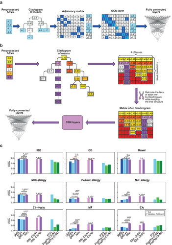
We trained 10 different models on different training partitions of the dataset, and for each model computed the AUC on the appropriate test set (a separate held-out test). Then we compared the average AUC (of the separate held-out test set over the 10 partitions) of gMic and gMic+v to the state-of-the-art results on the same datasets (Figure 1c). The AUC, when using only the structure in gMic was similar to one of the best naive models using the ASVs’ frequencies as tabular data (see Figure 1c). When combined with the ASVs’ frequencies, gMic+v outperformed existing methods in 4 out of 9 datasets by 0.05 on average (see Table 4 and Figure 1c).

Table 3. Sequential datasets details.

Dataset	Tag	Case	Control	Species	Range # of time steps	Ref
Diabimmune	Milk	53	150
	Peanut	9	194
	Egg	40	163
	All	72	131	87	1–33	^Citation75
DiGiulio case-control study	Preterm	11	29	321	3–158	^Citation76

Table 4. 10 CVs mean performances with standard deviation on external test sets; the std is the std among CV folds.

	iMic-CNN2	iMic-CNN1	gMic +v	gMic	FCN	PopPhy-CNN11	PopPhy-CNN2
IBD	0.961 ± 0.000	0.960 ± 0.000	0.956 ± 0.02	0.958 ± 0.014	0.94 ± 0.00	0.863 ± 0.02	0.834 ± 0.03
CD	0.931 ± 0.006	0.928 ± 0.000	0.936 ± 0.018	0.870 ± 0.023	0.807 ± 0.00	0.716 ± 0.03	0.751 ± 0.016
Ravel	0.946 ± 0.01	0.940 ± 0.000	0.977 ± 0.004	0.959 ± 0.006	0.965 ± 0.01	0.894 ± 0.00	0.898 ± 0.007
Cirrhosis	0.924 ± 0.01	0.896 ± 0.000	0.827 ± 0.013	0.847 ± 0.018	0.832 ± 0.03	0.633 ± 0.01	0.536 ± 0.09
Milk allergy	0.704 ± 0.03	0.704 ± 0.04	0.667 ± 0.104	0.707 ± 0.04	0.710 ± 0.03	0.557 ± 0.04	0.522 ± 0.05
Nut allergy	0.640 ± 0.01	0.659 ± 0.007	0.541 ± 0.081	0.499 ± 0.053	0.513 ± 0.05	0.599 ± 0.08	0.511 ± 0.05
Peanut allergy	0.588 ± 0.03	0.580 ± 0.03	0.535 ± 0.03	0.549 ± 0.073	0.575 ± 0.0	0.539 ± 0.02	0.541 ± 0.05
MF	0.641 ± 0.06	0.645 ± 0.06	0.446 ± 0.04	0.450 ± 0.054	0.51 ± 0.102	0.520 ± 0.06	0.527 ± 0.06
CA	0.681 ± 0.001	0.656 ± 0.01	0.507 ± 0.067	0.544 ± 0.144	0.535 ± 0.07	0.592 ± 0.04	0.610 ± 0.04

While gMic captures the relation between similar taxa, it still does not solve the sparsity problem. We thus suggest using iMic for a different combination of the relation between the structure of the cladogram and the taxa’s frequencies into an image and applying CNNs on this image to classify the samples (Figure 1b).

iMic is initiated with the same tree as gMic, but then instead of a GCN, the cladogram with the means in the vertices is projected to a two-dimensional matrix with eight rows (the number of taxonomic levels in the cladogram), and a column for each leaf.

Each leaf is set to its preprocessed frequency at the appropriate level and zero at the finer level (so if an ASV is at the genus level, the species level of the same genus is 0). Values at a coarser level (say at the family level) are the average values of the level below (a finer level-genus). For example, if we have three genera belonging to the same family, at the family level, the three columns will receive the average of the three values at the genus level (Figure 1b step 3).

As a further step to include the taxonomy in the image, columns were sorted recursively, so that taxa with more similar frequencies in the dataset would be closer using hierarchical clustering on the frequencies within a subgroup of taxa. For example, assume three sister taxa, $\mathit{taxo}{n}_a$, $\mathit{taxo}{n}_b$, and $\mathit{taxo}{n}_c$, the order of those three taxa in the row is determined by their proximity in the Dendrogram based on their frequencies (see Methods).

The test AUC of iMic was significantly higher than the state-of-the-art models in 6 out of 9 datasets by an average increase in AUC of 0.122 (Table 4 and Figure 1c). Specifically, in all the datasets that were tested, iMic had a significantly higher AUC than the 2 PopPhy models by 0.134 on average (corrected $\mathit{p}$-value $>0.001$ of two-sided T-test). For similar results on shotgun metagenomics datasets see Supp. Mat. Fig. S3.

iMic can also be applied to several different cohorts together. We used four different IBD cohorts, referred as IBD1.,⁴⁶ IBD2,⁵¹ IBD3,⁵² IBD4⁵³ Three of the cohorts were downloaded from.⁵⁴ Some of the datasets had no information at the species taxonomic level. Therefore, all the iMic images were created by the genus taxonomic level. Two learning tasks were applied: The first was a Leave One Dataset Out (LODO) task, where iMic was trained on three mixed cohorts and one cohort was left for testing. The second task was mixed learning based on the four cohorts. The LODO approach slightly reduced iMic’s accuracy, but still had high accuracy (AUC of 0.745 for the LODO IBD1, 0.659 for the LODO IBD2, 0.7 for the LODO IBD3, and 0.63 for the LODO IBD4). We also tested a mixed-learning setup where all datasets were combined with a higher AUC of 0.82 ± 0.01.

Often, non-microbial features are available beyond the microbiome. Those can be added to iMic by concatenating the non-microbial features to the flattened microbial output of the last CNN layer before the fully connected (FCN) layers. Adding non-microbial features even further improves the results of iMic when compared to a model without non-microbial features. Moreover, the incorporation of non-microbial features (such as sex, HDM, atopic dermatitis, asthma, age, and dose of allergen in the Allergy learning) leads to a higher accuracy than their incorporation in standard models (Table 5).

Table 5. Features can be added to iMic’s learning. Average AUCs of iMic-CNN2 with and without non-microbial features as well as average results of naive models with non-microbial features. The results are the average AUCs on an external test with 10 CVs $\pm$ their standard deviations (stds).

	iMic-CNN2 + non -microbial	iMic-CNN-only micro	RF+ non-microbial	SVC + non-microbial	LR + non-microbial	FCN + non-microbial
Milk allergy	$0.750\pm 0.04$	$0.704\pm 0.03$	$0.546\pm 0.03$	$0.478\pm 0.04$	$0.600\pm 0.03$	$0.661\pm 0.04$
Nut allergy	$0.680\pm 0.02$	$0.640\pm 0.01$	$0.630\pm 0.03$	$0.661\pm 0.02$	$0.603\pm 0.02$	$0.570\pm 0.03$
Peanut allergy	$0.633\pm 0.04$	$0.588\pm 0.03$	$0.582\pm 0.05$	$0.493\pm 0.05$	$0.427\pm 0.06$	$0.532\pm 0.07$

iMic best copes with the ML challenges above

As mentioned, microbiome-based ML is hindered by multiple challenges, including several representation levels, high sparsity, and high dimensional input vs a small number of samples. iMic simultaneously uses all known taxonomic levels. Moreover, it resolves sparsity by ensuring ASVs with similar taxonomy are nearby and averaged at finer taxonomic levels. As such, even if each sample has different ASVs, there is still common information at finer taxonomic levels. Using perturbations on the original samples, we demonstrate that iMic copes with each of these challenges better than existing methods.

• High sparsity. The microbiome data is extremely sparse with most of the taxa absent from most of the samples (see Supp. Mat. Fig. S1). iMic CNN averages over neighboring taxa. As such, even in the absence of some taxa, it can still infer their expected value from their neighbors. We define the initial sparsity rate of the data as the fraction of zero entries from the raw ASVs. The least sparse data was the Cirrhosis dataset ($72\mathrm{\%}$), followed by IBD, CD, CA, Ravel, and MF (all with a sparsity of $96\mathrm{\%}$). The sparsest dataset was Allergy ($98\mathrm{\%}$) which was not used in the sparsity analysis. We randomly zeroed entries to reach the required simulated sparsities (75, 80, 85, 90, and $95\mathrm{\%}$ for the Cirrhosis dataset) and (97, 98, and $99\mathrm{\%}$ for the others). iMic had the highest AUC and the least decrease in AUC when compared to other models (Fig. 2a–c). iMic is also significantly (after Benjamini Hochberg correction) more stable than gMic+v $(\mathit{p}$-value $<0.05)$. The results are similar for the other datasets (Supp. Mat. Fig. S5 and S6 for parallel results on the 10 CVs Supp. Mat. Fig. S9). The differences between iMic and all the other models in the AUC and in the decrease in AUC are also significant (after Benjamini Hochberg correction) in CD, CA, Cirrhosis and MF $(\mathit{p}$-value $<0.05)$.

  Figure 2. iMic copes with the ML challenges above better than other methods.

  (a) Average test AUC (over 10 CVs) as a function of the different sparsity levels, where the first point is the AUC of the original sparsity level (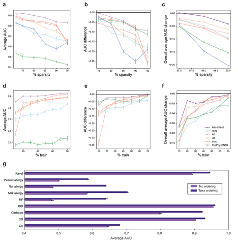$72\mathrm{\%}$, “baseline”) on the Cirrhosis dataset. iMic has the highest AUCs for all simulated sparsity levels (purple line). The error bars represent the standard errors. (b) Average change in AUC (AUC – baseline AUC) as a function of the sparsity level on the Cirrhosis dataset. (c) Overall average in AUC change in all the other datasets apart from Cirrhosis. (d) Average AUC as a function of the number of samples in the training set (Cirrhosis dataset). The error bars represent the standard errors of each model over the 10 CVs. (e) Average change in AUC (AUC – baseline AUC) as a function of the percent of samples in the training set. (f) Overall average AUC change over all the algorithms that managed to learn (baseline AUC $>0.55)$ as a function of the percent of samples in the training set. (g) Importance of ordering taxa. The x-axis represents the average AUC over 10 CVs and the y-axis represents the different datasets used. The deep purple bars represent the AUC on the images without taxa reordering, while the light purple bars represent the AUC on the images with the Dendrogram reordering with standard errors. All the differences between the AUCs are significant after Benjamini Hochberg correction $(\mathit{p}$-value $<0.001)$. All the AUCs are calculated on an external test set for each CV. Quite similar results were obtained on the 10 CVs.

  

• High dimensional input vs a small number of samples. By using CNNs with strides on the image microbial input, iMic reduces the model’s number of parameters in comparison to FCNs. iMic’s stability when changing the size of the training set was measured by reducing the training set size and measuring the AUC of iMic as well as the naive models (RF, SVC, LR and FCN). iMic was significantly (after Benjamini Hochberg correction) the most stable model $(\mathit{p}$-value $<0.05)$ in CA, CD, Cirrhosis, MF, and Allergy, among the models that succeeded to learn (baseline AUC $>0.55)$ as measured by the difference between the AUC of the reduced model and the baseline model, Figure 2 d-f. For the results on the other datasets as well, see Supp. Mat. Fig. S7 and S8 for parallel results on the 10 CVs Fig. S10.

• Several representation levels. iMic uses all taxonomic levels by adding the structure of the cladogram and translating it into an image. iMic further finds the best representation as an image by reordering the columns of the rows using Dendrogram clustering while maintaining the taxonomy structure. We confirmed that the reordering of sister taxa according to their similarity improves the performance in the classification task. The average AUCs of all the datasets are significantly higher (after Benjamini Hochberg correction) with taxa ordering vs no ordering $(\mathit{p}$-value $<0.001)$ (Figure 2g).

Classifier interpretation

Beyond its improved performance, iMic can be used to detect the taxa most associated with a condition. We used Grad-Cam (an explainable AI platform)⁵⁵ to estimate the part of the image used by the model to classify each class.⁵⁶ Formally, we estimated the gradient information flowing into the first layer of the CNN to assign importance and averaged the importance of the pixels for control and case groups separately (Figure 3 for the CD dataset, where we identify microbes to distinguish patients with CD from healthy subjects, and Supp. Mat. Fig. S11 - S13 for another phenotype). Interestingly, the CNN is most affected by the family and genus level (fifth row and sixth row in Figure 3). It used different taxa for the case and the control (see Figure 3c,d). To find the microbes that most contributed to the classification, we projected the computed Grad-Cam values back to the cladogram (Figure 3a,b). In the CD dataset, Proteobacteria are characteristic of the CD group, in line with the literature. This phylum is proinflammatory and associated with the inflammatory state of CD and overall microbial dysbiosis.⁵⁷ Also in line with previous findings is the family Micrococcaceae associated with colonial CD⁵⁸ and even with mesenteric adipose tissue microbiome in CD patients.⁵⁹ The control group was characterized by the family Bifidobacteriaceace, known for its anti-inflammatory properties, pathogen resistance, and overall improvement of host state,^60,61 and by Akkermansia, which is a popular candidate in the search for next-generation probiotics due to its ability to promote metabolism and the immune function.⁶²

Figure 3. Interpretation of iMic’s results.

(a, b) Cladogram projections: To visualize the taxa contributing to each class, the healthy class (a) and the CD class (b), we projected the most significant microbes back on the cladogram. The purple points on the cladograms represent taxa that are in the top decile of the gradients. The taxa in bold are important taxa that are consistent with the literature. (c, d) Grad-Cam images: Each image represents the average contribution of each input value to the gradients of the neural network back-propagation, as computed by the Grad-Cam algorithm. We put the Grad-Cam after the first CNN layer. The results presented here are from the CD dataset. (c) represents the average gradients for the healthy subjects of the cohort and (d) represents the average gradients for the CD subjects. The color reflects the average values of the gradients, such that the blue colors represent low gradients, and the yellow colors represent the high gradients, using the ‘viridis’ colormap. The differences between the two heatmaps represent the contribution of different taxa to the prediction of different phenotypes. Note that the main contribution to the classification is at the genus and family level (rows 6 and 5). Similar results were obtained for the other datasets (Fig. S11 in Supp. Mat.) (e-h). Interpretation tests on the CD dataset (e), the IBD dataset (f), the Cirrhosis dataset (g), and the Ravel dataset (h). Average AUC values over 10 CVs on the external test set. The x-axis represents the fraction of removed columns. The dark bars represent the performance when all of the columns with Grad-Cams values lower than this fraction have been removed and the light bars represent the performance when the columns with scores above this fraction have been removed. The black line represents the average AUC over 10 CVs of the original model with all the input columns. Results from the other datasets were similar, see Supp. Mat Fig. S11. Removing the top scoring columns always reduced the performance. Removing the bottom scoring columns increases or does not change the AUC.

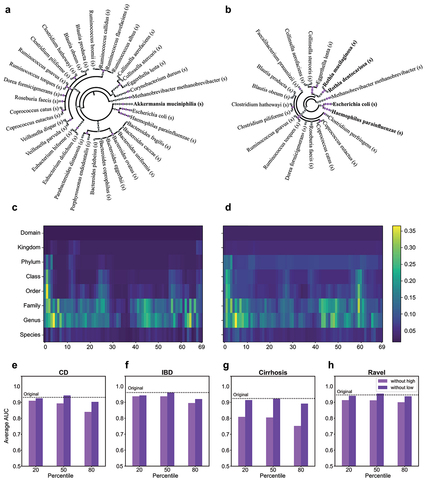
To test that the significant taxa contribute to the classification, we defined “good columns” and “bad columns”. A “good column” is defined as a column where the sum of the averaged Grad-Cam in the case and control groups is in the top $\mathit{k}$ percentiles, and a “bad column” is defined by the lowest $\mathit{k}$ percentiles. When removing the “good columns”, the test AUC was reduced by 0.07 on average, whereas when the “bad columns” were removed, the AUC slightly improved by 0.006 (Figure 3e–f; for all the other datasets, see Supp. Mat. Fig. S14).

Sensitivity analysis

To ensure that the improved performance is not the result of hyperparameter tuning, we checked the impact on the AUC of fixing all the hyperparameters but one and changing a specific hyperparameter by increasing or decreasing its value by 10–30%. The difference between the AUC of the optimal parameters and all the varied combinations is low with a range of $0.03+/-0.03$ (Supp. Mat. Fig. S15), smaller than the increase in AUC of iMic compared to other methods.

Temporal microbiome

iMic translates the microbiome into an image. One can use the same logic and translate a set of microbes to a movie to classify sequential microbiome samples. We used iMic to produce a 2-dimensional representation for the microbiome of each time step and combined those into a movie of the microbial images (see Supp. Mat. for such a movie). We used a 3D Convolutional Neural Network (3D-CNN) to classify the samples. We applied 3D-iMic to two different previously studied temporal microbiome datasets (Table 3), comparing our results to the state-of-the-art – a one-dimensional representation of taxon-NN PhyLoSTM.⁶³ The AUC of 3D-iMic is significantly higher after Benjamini Hochberg correction ($\mathit{p}-\mathit{value}<0.0005$) than the AUC of PhyloLSTM over all datasets and tags (Figure 4b).

Figure 4. 3D learning.

(a) iMic 3D Architecture: The ASV frequencies of each snapshot are preprocessed and combined into images as in the static iMic. The images from the different time points are combined into a 3D image, which is the input of a 3-dimensional CNN followed by two fully connected layers that return the predicted phenotype. (b) Performance of 3D learning vs PhyLoSTM. The AUCs of the 3D-iMic are consistently higher than the AUCs of the phyLoSTM on all the tags and datasets we checked $(\mathit{n}=5)$. The standard errors among the CVs are also shown. phyLoSTM is the current state-of-the-art for these datasets (two-sided T-test, $\mathit{p}$-value $<0.0005$). To visualize the three-dimensional gradients (as in Figure 3), we studied a CNN with a time window of 3 (i.e., 3 consecutive images combined using convolution). We projected the Grad-Cam images to the R, G, and B channels of an image. Each channel represents another time point where R = earliest, G = middle, and B = latest time point. (c,d) Images after Grad-Cam: Each pixel represents the value of the backpropagated gradients after the CNN layer. The 2-dimensional image is the combination of the three channels above. (i.e., the gradients of the first/second/third time step are in red/green/blue). The left image is for normal birth subjects in the DiGiulio dataset, and the right image is for pre-term birth subjects. (e,f) Grad-Cam projection. Projection of the above heatmaps on the cladogram as in Figure 3. The taxa in bold are important taxa that are consistent with the literature.

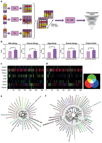
To understand what temporal features of the microbiome were used for the classification, we calculated again the heatmap of backwards gradients of each time step separately using Grad-Cam. We focused on CNNs with a window of 3-time points, and represented the heatmap of the contribution of each pixel in each time step in the $\mathit{R},$ $\mathit{G},$ and $\mathit{B}$ channels, producing an image that combines the cladogram and time effects and projected this image on the cladogram. We used this visualization on the DiGiulio case-control study of preterm and full-term neotnates’ microbes, and again projected the microbiome on the cladogram, showing the RGB representation of the contribution to the classification. Again, characteristic taxa of preterm infants (Figure 4c,e) and full-term infants (Figure 4d,f) were in line with previous research. Here preterm infants were characterized by TM7, common in the vaginal microbiota of women who deliver preterm.^3,64 Staphylococci have also been identified as the main colonizers of the pre-term gut.^65,66 Full-term infants were characterized by a number of Fusobacteria taxa. Bacteria of this phylum are common at this stage of life.⁶⁷

Discussion

The application of ML to microbial frequencies, represented by 16S rRNA or shotgun metagenomics ASV counts at a specific taxonomic level is affected by three types of information loss – ignoring the taxonomic relationships between taxa, ignoring sparse taxa present in only a few samples, and ignoring rare taxa (taxa with low frequencies) in general.

We have first shown that the cladogram is highly informative through a graph-based approach named gMic. We have shown that even completely ignoring the frequency of the different taxa, and only using their absence or presence can lead to highly accurate predictions on multiple ML tasks, typically as good or even better than the current state-of-the-art.

We then propose an image-based approach named iMic to translate the microbiome to an image where similar taxa or proximal are close to each other and apply CNN to such images to perform ML tasks. We have shown that iMic produces higher precision predictions (as measured by the test set AUC Figure 1c and Supp. Mat. Fig. S4) than current state-of-the-art microbiome-based ML on a wide variety of ML tasks. We then have further shown that iMic is less sensitive to the limitations above. Specifically, iMic is less sensitive to the rarefaction of the ASV in each sample. Removing random taxa from samples had the least effect on iMic’s accuracy in comparison to other methods. Similarly, iMic is most robust to the removal of full samples. Finally, iMic explicitly incorporates the cladogram. Removing the cladogram information reduces the classification accuracy. iMic also improves the state-of-the-art in microbial dynamic prediction (phyLoSTM) by treating the dynamic microbiome as a movie and applying 3D-CNNs. We found that a typical window of three snapshots was enough to extract the information from dynamic microbiome samples.

An important advantage of iMic is the production of explainable models. Moreover, treating the microbiome as images opens the door to many vision-based ML tools, such as: transfer learning from pre-trained models on images, self-supervised learning, and data augmentation. Combining iMic with an explainable AI methodology highlights microbial taxa associated with a group with different phenotypes. Those are in line with relevant taxa previously noted in the literature.

While iMic handles many limitations of existing methods, it still has important limitations and arbitrary decisions. iMic orders taxa by hierarchically using the cladogram, and within the cladogram, based on the similarity between the counts among neighboring microbes. This is only one possible clustering method and other orders may be used that may further improve the accuracy. Also, we used a simple network structure; however, much more complex structures could be used. Still iMic shows that the detailed incorporation of the structure is crucial for microbiome-based ML.

Other limitations of iMic include: A) While iMic improves ML, it does not produce a distance metric, and we will attempt to develop one. B) It learns on the full dataset and does not directly define specific single microbes linked to the outcome. This is addressed by applying explainable AI methods (specifically Grad-Cam) to the iMic results. C) As is the case for any ML, it does not provide causality. Still composite biomarkers, based on a full microbiome repertoire are possible.

The development of microbiome-based biomarkers (micmarkers) is one of the most promising routes for easy and large-scale detection and prediction. However, while many microbiome-based prediction algorithms have been developed, they suffer from multiple limitations, which are mainly the result of the sparsity and the skewed distribution of taxa in each host. iMic and gMic are important steps in the translation of microbiome samples from a list of single taxa to a more holistic view of the full microbiome. We are now developing multiple microbiome-based diagnostics, including a prediction of the effect of the microbiome composition on Fecal Microbiota Transplants (FMT outcomes).⁶⁸ We have previously shown that the full microbiome (and not specific microbes) can be used to predict pregnancy complications.⁶⁹ We propose that either the tools developed here or tools using the same principles can be used for high-accuracy clinical microbiome-based biomarkers.

Methods

Preprocessing

We preprocessed the 16S rRNA gene sequences of each dataset using the MIPMLP pipeline.⁴⁹ The preprocessing of MIPMLP contains four stages: merging similar features based on the taxonomy, scaling the distribution, standardization to z-scores, and dimension reduction. We merged the features at the species taxonomy by Sub-PCA before using all the models. We performed log normalization as well as z-scoring on the patients. No dimension reduction was used at this stage. For the LODO and mixed predictions of the IBD datasets, the features were merged into the genus taxonomic level, since the species of 3 of the cohorts were not available.

All models preprocessing

Sub-PCA merging in MIPMLP

A taxonomic level (e.g., species) is set. All the ASVs consistent with this taxonomy are grouped. A PCA is performed on this group. The components which explain more than half of the variance are added to the new input table. This was applied for all models apart from the PopPhy models.³¹

Log normalization in MIPMLP

We logged (10 base) scale the features element-wise, according to the following formula:

(1) $x_{\mathit{i},\mathit{j}}\to log(x_{\mathit{i},\mathit{j}}+\in ),$(1)

where $\in$ is a minimal value $(=0.1)$ to prevent log of zero values. This was applied for all models apart from the PopPhy models.

PopPhy preprocessing

Sum merging in MIPMLP

A level of taxonomy (e.g., species) is set. All the ASVS consistent with this taxonomy are grouped by summing them. This was applied to the PopPhy models.

Relative normalization in MIPMLP

To normalize each taxon through its relative frequency:

(2) $x_{\mathit{i},\mathit{j}}=\frac{{\mathit{x}}_{\mathit{i},\mathit{j}}}{{\sum }_{k=1}^n{x}_{\mathit{k},\mathit{j}}},$(2)

we normalized the relative abundance of each taxon $\mathit{j}$ in sample $\mathit{i}$ by its relative abundance across all $\mathit{n}$ samples. This was applied only to the PopPhy models.

Current methods

We compared gMic and iMic models’ results to six current methods: ASV frequency two layers fully connected neural network (FCN). The FCN was implemented via the pytorch lightening platform.⁷⁰ Other simple popular value-based approaches are: Random Forest (RF).,⁷¹ Support Vector Classification (SVC)⁷¹ and Logistic Regression (LR)⁷¹ All the simple approaches were implemented by the sklearn functions:

sklearn.ensemble.RandomForestClassifier, sklearn.svm.SVC and

sklearn.linear_model.LogisticRegression, respectively. To evaluate the performance by using only the values. The other two models were the previous state-of-the-art models that use structure, PopPhy,³¹ followed by 1 convolutional layer or 2 convolutional layers and their output followed by FCNs (2 layers). The models’ inputs were the ASVs merged at the species level by the sum method followed by a relative normalization as described in the original paper. We used the original PopPhy code from Reiman’s GitHub.

Notations

To clarify the notations, we attach a detailed table, with all notations (Table 6).

Table 6. Notations.

$\mathit{b}$	ASVs preprocessed vector (only the leaves of the cladogram)
$\mathit{R}$	Raw representation matrix
$\hat{R}$	Rearranged representation matrix
$\mathit{l}$	A taxonomic level (Super-kingdom, Phylum, Class, Order, Family, Genus, Species)
$\mathit{N}$	Number of leaves of the cladogram of means
$C_{\mathit{l},\mathit{i}}$	Hierarchical cluster number $\mathit{i}$ in level $\mathit{l}$
$\mathit{A}$	Adjacency matrix of graph
$\mathit{\sigma }$	Activation function
$\mathit{W}$	Weight matrix in neural network
$\mathit{I}$	Identity matrix
$\mathit{v}$	ASVs frequency vector (all the cladogram’s vertices, and not only the leaves, in contrast with $\mathit{b}$ above)

iMic

The iMic’s framework consists of three algorithms:

• Populating the mean cladogram.

• Cladogram2Matrix.

• CNN.

Given a vector of log-normalized ASVs frequencies merged to taxonomy 7 - $\mathit{b}$, each entry of the vector, $b_i$ represents a microbe at a certain taxonomic level. We built an average cladogram, where each internal node is the average of its direct children (see Populating mean cladogram algorithm and Figure 1b). Once the cladogram was populated, we built the representation matrix. We created a matrix $\mathit{R}\in {\mathbb{R}}^{8\times \mathit{N}}$, where N was the number of leaves in the cladogram and 8 represents the eight taxonomic levels, such that each row represents a taxonomic level.

We added the values layer by layer, starting with the values of the leaves. If there were taxonomic levels below the leaf in the image, they were populated with zeros. Above the leaves, we computed for each taxonomic level the average of the values in the layer below (see Figure 1b step 3). If the layer below had $\mathit{k}$ different values, we set the average to all $\mathit{k}$ positions in the current layer. For example, if there were three species within one genus with values of 1,3 and 3. We set a value of 7/3 to the three positions at the genus level including these species.

We reordered the microbes at each taxonomic level (row) to ensure that similar microbes are close to each other in the produced image. Specifically, we built a Dendrogram based on the Euclidean distances as a metric using complete linkage on the columns, relocating the microbes according to the new order while keeping the phylogenetic structure. The order of the microbes was created recursively. We started by reordering the microbes on the phylum level, relocating the phylum values with all their sub-tree values in the matrix. Then we built a Dendrogram of the descendants of each phylum separately, reordering them and their sub-tree in the matrix. We repeated the reordering recursively until all the microbes in the species taxonomy of each phylum were ordered. (see Reordering algorithm and see Figure 1b step 4).

Table

Algorithm 1: Populating mean cladogram algorithm

1 Input: Cladogram, $\mathit{G}=(\mathit{V},\mathit{E})$, a preprocessed ASVs vector, $\mathit{b}$ 2 Output: A populated cladogram of means, $\mathit{G}$ 3 for $\mathit{l}$ from the maximum cladogram depth to 0 do 4 for each node, $\mathit{v}$, in layer,$\mathit{l}$ do 5 if the layer of $\mathit{v}$ is in $\mathit{b}$ then 6 Assign node $\mathit{v}$ the value from $\mathit{b}$ 7 if $\mathit{v}$ has any children then 8 Assign its children mean to $\mathit{v}$ 9 return $\mathit{G}$

Table

Algorithm 2: Cladogram2matrix algorithm

1 Input: A populated cladogram of means $\mathit{G}=\mathit{V},\mathit{E}$ 2 Output: A matrix $\mathit{R}$ 3 Construct a zero matrix $\mathit{R}$ with the number of rows equal to the layers of the cladogram and the number of columns equal to the number of leaves in the cladogram 4 $\mathit{C}\leftarrow$ Root Node of $\mathit{G}$ 5 for $\mathit{j}$ from 0 to the number of layers of $\mathit{G}$ do 6 $\mathit{i}\leftarrow 0$ 7 $\mathit{Q}\leftarrow \mathit{emptyQueue}$ 8 for each node $\mathit{v}\in \mathit{C}$ do 9 Notice: every node is a sub-tree 10 if node does not have any children then 11 $\mathit{R}(\mathit{i},\mathit{j})\leftarrow$ abundance of node $\mathit{v}$ 12 else 13 for $\mathit{k}$ from 1 to number of leaves of node $\mathit{v}$ do 14 $\mathit{R}(\mathit{i},\mathit{j})\leftarrow$ abundance of node $\mathit{v}$ 15 $\mathit{i}\leftarrow \mathit{i}+1$ 16 Push children of node v into queue $\mathit{Q}$ 17 $\mathit{i}\leftarrow \mathit{i}+1$ 18 $\mathit{C}\leftarrow \mathit{Q}$ 19 return R

Table

Algorithm 3: Reordering algorithm, REA

1 Input: $\mathit{R}\in {\mathbb{R}}^{8\times \mathit{N}}$, $\mathit{l}$ level of taxonomy 2 Output: $\hat{R}$, rearranged matrix $\mathit{R}$ 3 $\hat{R}$ $\leftarrow \mathit{\varphi }$ 4 Annotate: R in level l: $b_1,b_2,\dots ,b_N$ 5 $C_{\mathit{l},1},\dots ,C_{\mathit{l},\mathit{k}}$ $\leftarrow \mathit{Dendrogram}(b_1,b_2,\dots ,b_N)$ 6 Temp $\leftarrow \mathit{\varphi }$ 7 for Cluster in $C_{\mathit{l},1},\dots ,C_{\mathit{l},\mathit{k}}$ do 8 for taxa in Cluster do 9 Append taxa column to Temp if $\mathit{l}<8$ then 10 Temp $\leftarrow \mathit{REA}(\mathit{Temp},\mathit{l}+1)$ 11 Append Temp to $\hat{R}$ 12 return $\hat{R}$

2-dimensional CNN

The microbiome matrix was used as the input to a standard CNN.⁷² We tested both one and two convolution layers (when three convolution layers or more were used, the models suffered from overfitting). Our loss function was the binary cross entropy. We used L1 regularization. We also used a dropout after each layer, the strength of the dropout was controlled by a hyperparameter. For each dataset, we chose the best activation function among RelU, elU, and tanh. We also used strides and padding. All the hyperparameter ranges as well as the chosen and fixed hyperparameters can be found in the Supplementary Material (Table S1-S4). In order to limit the number of model parameters, we added max pooling between the layers if the number of parameters was higher than 5000. The output of the CNNs was the input of a two-layer, fully connected neural network.

gMic and gMic+v

The cladogram and the gene frequency vector were used as the input. The graph was represented by the symmetric normalized adjacency matrix, which was denoted $\tilde{A}$ as can be seen in the following equations:

(3) $\tilde{A}=D^{-\frac{1}{2}}\mathit{A}{D}^{-\frac{1}{2}}$(3)

(4) $\mathit{D}\mathrm{is}\mathrm{a}\mathrm{diagonal}\mathrm{matrix}\mathrm{such}\mathrm{that}{D}_{\mathit{ii}}=\sum _j{A}_{\mathit{ij}}$(4)

The loss function was binary cross entropy. In this model, we used L2 regularization as well as a dropout.

gMic

The cladogram was built and populated as in iMic. In gMic, a GCN layer was applied to the cladogram. The output of the GCN layer was the input to a fully connected neural network (FCN) as in:

(5) $\mathit{\sigma }((\tilde{A}+\mathit{\alpha }\cdot \mathit{I})\cdot \mathit{sign}(\mathit{v})\cdot \mathit{W})\Rightarrow \mathit{FCN}$(5)

where $\mathit{v}$ is the ASVs frequency vector (all the cladogram’s vertices, and not only the leaves, in contrast with b above), $\mathit{sign}(\mathit{v})$ is the same vector where all positive values were replaced by 1 in the gene frequency vector (i.e., the values are ignored). $\mathit{\alpha }$ is a learned parameter, regulating the importance given to the vertices’ values against the first neighbors, $\mathit{W}$ is the weight matrix in the neural network, and $\mathit{\sigma }$ is the activation function. The architecture of the FCN is common in all datasets. The hyperparameters may be different (for further information see Supp. Mat. Table S3): two hidden layers, each followed by an activation function (see Supp. Mat.).

gMic+v

gMic+v is equivalent to gMic, with the only exception that the positive values were not set to 1.

Data

We used nine different tags from six different datasets of 16S rRNA ASVs to evaluate iMic and gMic+v. 4 datasets were contained within the Knights Lab ML repository:⁷³ Cirrhosis, Caucasians and Afro Americans (CA), Male vs Female (MF) and Ravel vagina.

• The Cirrhosis dataset was taken from a study of 68 Cirrhosis patients and 62 healthy subjects.⁷⁴

• The MF dataset was a part of the human microbiome project (HMP) and contained 98 males and 82 females.⁴⁷

• The CA dataset consisted of 104 Caucasian and 96 Afro-American vaginal samples.⁴⁸

• The Ravel dataset was based on the same cohort as the CA, but checked another condition of the Nugent score.⁴⁸ The Nugent score is a Gram stain scoring system for vaginal swabs to diagnose bacterial vaginosis.

• The IBD dataset contains 137 samples with inflammatory bowel disease (IBD), including Crohn’s disease (CD) and ulcerative colitis (UC), and 120 healthy samples as controls. We also used the same dataset for another task of predicting only CD from the whole society, where there were 94 with CD and 163 without CD.⁴⁶

• The Allergy dataset is a cohort of 274 subjects. We tried to predict three different outcomes. The first is having or not having a milk allergy, where there are 74 subjects with a milk allergy and 200 without. The second is having or not having a nut (walnut and hazelnut) allergy, where there are 53 with a nut allergy and 221 without. The third is having or not having an allergy to peanut, where 79 have a peanut allergy and 195 do not.⁵

For the comparisons with TopoPhy, we applied iMic to the shotgun metagenomes datasets presented in TopoPhy³³ from MetAML, including a Cirrhosis dataset with 114 cirrhotic patients and 118 healthy subjects (“Cirrhosis−2”), an obesity dataset with 164 obese and 89 non-obese subjects (“BMI”), a T2D dataset of 170 T2D patients and 174 control samples (“T2D”).

For the comparisons with TaxoNN, we applied iMic to the datasets presented in TaxoNN’s paper (Cirrhosis−2 and T2D).

For the comparison with DeepEn-Phy,³⁴ we applied iMic on the Guangdong Gut Microbiome Project (GGMP) – a large microbiome-profiling study conducted in Guangdong Province, China, with 7009 stool samples (2269 cases and 4740 controls to classify smoking status). GGMP was downloaded from the Qiita platform. We used the results supplied by TopoPhy, TaxoNN, and DeepEn-Phy, and did not apply them to other datasets, since their codes were either missing, or did not work as is, and we did not want to make assumptions regarding the corrections required for the code.

We also used two sequential datasets to evaluate iMic-CNN3 (Table 3).

• The first dataset was the DIABIMMUNE three-country cohort with food allergy outcomes (Milk, Egg, Peanut, and Overall). This cohort contained 203 subjects with 7.1428 time steps on average.⁷⁵

• The second dataset was a DiGiulio case-control study. This was a case-control study comprised of 40 pregnant women, 11 of whom delivered preterm serving as the outcome. Overall, in this study, there were 3767 samples with 1420 microbial samples from four body sites: vagina, distal gut, saliva, and tooth/gum. In addition to bacterial taxonomic composition, clinical and demographic attributes included in the dataset were gestational or postpartum day when the sample was collected, race, and ethnicity.⁷⁶

Statistics – comparison between models

To compare the performances of the different models, we performed a one-way ANOVA test (from scipy.stats in python) on the test AUC from the 10 CVs of all the models. If the ANOVA test was significant, we also performed a two-sided T-test between iMic and the other models and between the two CNNs on the iMic representation. Correction for multiple testing (Benjamini – Hochberg procedure, Q) was applied when appropriate with a significance level of $\mathit{Q}<0.05$. (see Figure 1c). Only significant results after a correction were reported.

To compare the performance on the sparsity and high dimensions challenges, we first performed a two-way ANOVA with the first variable being the sparsity and the second variable being the model on the test AUC over 10 CVs. Only when the ANOVA test was significant (all the datasets in our case), we also performed a two-sided T-test between iMic and the naive models. Correction for multiple testing (Benjamini – Hochberg procedure, $\mathit{Q}$) was applied when appropriate with significance defined at $\mathit{Q}<0.05$. All the tests were also checked on the independent 10 CVs of the models on the validation set and the results were similar. Note that in contrast with the test set estimates, this test may be affected by parameter tuning.

Experimental setup

Splitting data to training, validation and test sets

Following the initial preprocessing, we divided the data using an external stratified test, such that the distribution of positives and negatives in the training set and the held-out test set would be the same and would preserve the patient identity in cases and controls into training, test, and validation sets. This ensures that the same patient cannot be simultaneously in the training and the test set. The external test was always the same 20% of the whole data. The remaining 80% were divided into the internal validation (20% of the data) and the training set (60%). In cross-validations, we changed the training and validations, but not the test.

Hyperparameters tuning

We computed the best hyperparameters for each model using a 10-fold CV⁷⁷ on the internal validation. We chose the hyperparameters according to the average AUC on the 10 validations. The platform we used for the optimization of the hyperparameters is NNI (Neural Network Intelligence).⁵⁰ The hyperparameters tuned were: the coefficient of the L1 loss, the weight decay (L2-regularization), the activation function (RelU,elU or tanh, which makes the model non-linear), the number of neurons in the fully connected layers, dropout (a regularization method which zeros the neurons in the layers in the dropout’s probability), batch size and learning rate. For the CNN models, we also included the kernel sizes as well as the strides and the padding as hyperparameters. The search spaces we used for each hyperparameter were: L1 coefficient was chosen uniformly from [0,1]. Weight decay was chosen uniformly from [0,0.5]. The learning rate was one of [0.001,0.01,0.05]. The batch size was,^32,66 218, 256]. The dropout was chosen universally from [0,0.05,0.1,0.2,0.3,0.4,0.5]. We chose the best activation function from RelU, ElU and tanh. The number of neurons was proportional to the input dimension. The first linear division factor from the input size was chosen randomly from.^1,11 The second layer division factor was chosen from.^1,6 The kernel sizes were defined by two different hyperparameters, a parameter for its length and its width. The length was in the range of^1,8 and the width was in the range of.^1,20 The strides were in the range of^1,9 and the channels were in the range of.^1,16 For the classical ML models, we used a grid search instead of the NNI platform. The evaluation method was similar to the other models. The hyperparameters of the RF were: The number of trees in the range of,^10,52100,150,200] and the function to measure the quality of a split (one of “gini”, “entropy”, “log_loss”). The hyperparameters of the SVC were: the regularization parameter in the range of [0.0,0.1,0.2,0. 3,0.4,0.5,0.6,0.7,0.8,0.9,1.0], and the kernel (one of “linear”, “poly”, “rbf”, “sigmoid”). The best hyperparameters for each dataset can be found in Supp. Mat. Table S5.

Contribution

OS developed the methods, implemented them, ran the code, and created all the figures, as well as prepared an initial draft of the text. HI implemented gMic and helped in writing parts of the text. YL and OK supervised the work and wrote parts of the text. OK and ST interpreted the biological relevance of the results. ST wrote parts of the text.

Acknowledgments

We thank Miriam Beller for the English editing. OK is supported by the European Research Council (ERC) under the European Union’s Horizon 2020 research and innovation program (Grant agreement ERC-2020-COG No. 101001355). We thank Maayan Harel (Maayan Visuals) for her graphical contribution.

Disclosure statement

No potential conflict of interest was reported by the author(s).

Data availability statement

All datasets are available at https://github.com/oshritshtossel/iMic/tree/master/Raw_data.

Supplementary material

Supplemental data for this article can be accessed online at https://doi.org/10.1080/19490976.2023.2224474

Additional information

Funding

OS was supported by the DSI-BIU grant for outstanding students in data science. YL was supported by ISF 870/20 and the Ministry of Health Preventive medicine 1/20 and OK was supported by the European Union’s Horizon 2020 research and innovation program (Grant agreement ERC-2020-COG No. 101001355).

References

- Bunyavanich S, Shen N, Grishin A, Wood R, Burks W, Dawson P, Jones SM, Leung DYM, Sampson H, Sicherer S, et al. Early-life gut microbiome composition and milk allergy resolution. J Allergy Clin Immunol. 2016;138(4):1122–22. doi:10.1016/j.jaci.2016.03.041.
- Lee K. Hung, Guo J, Song Y, Ariff A, O’sullivan M, Hales B, Mullins BJ, Zhang G. Dysfunctional gut microbiome networks in childhood IgE-mediated food allergy. Int J Mol Sci. 2021;22(4):2079. doi:10.3390/ijms22042079.
- Fettweis JM, Serrano MG, Paul Brooks J, Edwards DJ, Girerd PH, Parikh HI, Huang B, Arodz TJ, Edupuganti L, Glascock AL, et al. The vaginal microbiome and preterm birth. Nat Med. 2019;25(6):1012–1021. doi:10.1038/s41591-019-0450-2.
- Michail S, Durbin M, Turner D, Griffiths AM, Mack DR, Hyams J, Leleiko N, Kenche H, Stolfi A, Wine E. Alterations in the gut microbiome of children with severe ulcerative colitis. Inflamm Bowel Dis. 2012;18(10):1799–1808. doi:10.1002/ibd.22860.
- Goldberg MR, Mor H, Magid Neriya D, Magzal F, Muller E, Appel MY, Nachshon L, Borenstein E, Tamir S, Louzoun Y, et al. Microbial signature in IgE-mediated food allergies. Genome Med. 2020;12(1):1–18. doi:10.1186/s13073-020-00789-4.
- Binyamin D, Werbner N, Nuriel-Ohayon M, Uzan A, Mor H, Abbas A, Ziv O, Teperino R, Gutman R, Koren O. The aging mouse microbiome has obesogenic characteristics. Genome Med. 2020;12(1):1–9. doi:10.1186/s13073-020-00784-9.
- Ward DM, Weller R, Bateson MM. 16s rRNA sequences reveal numerous uncultured microorganisms in a natural community. Nature. 1990;345(6270):63–65. doi:10.1038/345063a0.
- Poretsky R, Rodriguez-R LM, Luo C, Tsementzi D, Konstantinidis KT, Rodriguez-Valera F. Strengths and limitations of 16s rRNA gene amplicon sequencing in revealing temporal microbial community dynamics. PLos One. 2014;9(4):e93827. doi:10.1371/journal.pone.0093827.
- Ross AB, Bruce SJ, Blondel-Lubrano A, Oguey-Araymon S, Beaumont M, Bourgeois A, Nielsen-Moennoz C, Vigo M, Fay L-B, Kochhar S, et al. A whole-grain cereal-rich diet increases plasma betaine, and tends to decrease total and ldl-cholesterol compared with a refined-grain diet in healthy subjects. Br J Nutr. 2011;105(10):1492–1502. doi:10.1017/S0007114510005209.
- Gupta VK, Kim M, Bakshi U, Cunningham KY, Davis JM III, Lazaridis KN, Nelson H, Chia N, Sung J. A predictive index for health status using species-level gut microbiome profiling. Nat Commun. 2020;11(1):4635. doi:10.1038/s41467-020-18476-8.
- Wang J, Zheng J, Shi W, Du N, Xiaomin X, Zhang Y, Peifeng J, Zhang F, Jia Z, Wang Y, et al. Dysbiosis of maternal and neonatal microbiota associated with gestational diabetes mellitus. Gut. 2018;67(9):1614–1625. doi:10.1136/gutjnl-2018-315988.
- Prodan A, Tremaroli V, Brolin H, Zwinderman AH, Nieuwdorp M, Levin E, Seo J-S. Comparing bioinformatic pipelines for microbial 16s rRNA amplicon sequencing. PLoS One. 2020;15(1):e0227434. doi:10.1371/journal.pone.0227434.
- Darcy JL, Washburne AD, Robeson MS, Prest T, Schmidt SK, Lozupone CA. A phylogenetic model for the recruitment of species into microbial communities and application to studies of the human microbiome. Isme J. 2020;14(6):1359–1368. doi:10.1038/s41396-020-0613-7.
- Qiu Y-Q, Tian X, Zhang S. Infer metagenomic abundance and reveal homologous genomes based on the structure of taxonomy tree. IEEE/ACM Trans Comput Biol Bioinf. 2015;12(5):1112–1122. doi:10.1109/TCBB.2015.2415814.
- Asgari E, Münch PC, Lesker TR, McHardy AC, Mofrad MRK, Birol I. Ditaxa: nucleotide-pair encoding of 16s rRNA for host phenotype and biomarker detection. Bioinformatics. 2019;35(14):2498–2500. doi:10.1093/bioinformatics/bty954.
- Lee H, Lee HK, Min SK, Lee WH. 16s rDNA microbiome composition pattern analysis as a diagnostic biomarker for biliary tract cancer. World J Surg Oncol. 2020;18(1):1–10. doi:10.1186/s12957-020-1793-3.
- Turjeman S, Koren O. Using the microbiome in clinical practice. Microb Biotechnol. 2021;15(1):129–134. doi:10.1111/1751-7915.13971.
- Nishijima S, Suda W, Oshima K, Kim S-W, Hirose Y, Morita H, Hattori M. The gut microbiome of healthy Japanese and its microbial and functional uniqueness. DNA Res. 2016;23(2):125–133. doi:10.1093/dnares/dsw002.
- VijiyaKumar K, Lavanya B, Nirmala I, Caroline SS. Random forest algorithm for predicting chronic diabetes disease. 2019 IEEE International Conference on System, Computation, Automation and Networking (ICSCAN). 2019. p. 1–5. doi:10.1109/ICSCAN.2019.8878802.
- Jacobs JP, Goudarzi M, Singh N, Tong M, McHardy IH, Ruegger P, Asadourian M, Moon B-H, Ayson A, Borneman J, et al. A disease-associated microbial and metabolomics state in relatives of pediatric inflammatory bowel disease patients. Cell Mol Gastroenterol Hepatol. 2016;2(6):750–766. doi:10.1016/j.jcmgh.2016.06.004.
- Ben Izhak M, Eshel A, Cohen R, Madar-Shapiro L, Meiri H, Wachtel C, Leung C, Messick E, Jongkam N, Mavor E, et al. Projection of gut microbiome pre-and post-bariatric surgery to predict surgery outcome. mSystems. 2020;6(3):e01367–20. doi:10.1128/mSystems.01367-20.
- Oudah M, Henschel A. Taxonomy-aware feature engineering for microbiome classification. BMC Bioinform. 2018;19(1):1–13. doi:10.1186/s12859-018-2205-3.
- Albanese D, De Filippo C, Cavalieri D, Donati C, Brem R. Explaining diversity in metagenomic datasets by phylogenetic-based feature weighting. PLoS Comput Biol. 2015;11(3):e1004186. doi:10.1371/journal.pcbi.1004186.
- Xiao J, Chen L, Yue Y, Zhang X, Chen J. A phylogeny-regularized sparse regression model for predictive modeling of microbial community data. Front Microbiol. 2018;9:3112. doi:10.3389/fmicb.2018.03112.
- Ditzler G, Polikar R, Rosen G. Multi-layer and recursive neural networks for metagenomic classification. IEEE Trans Nanobioscience. 2015;14(6):608–616. doi:10.1109/TNB.2015.2461219.
- Krizhevsky A, Sutskever I, Hinton GE. Imagenet classification with deep convolutional neural networks. Adv Neural Inf Process Syst. 2012;25:1097–1105.
- Kipf TN, Welling M. Semi-supervised classification with graph convolutional networks. arXiv Preprint arXiv: 1609 02907. 2016.
- Park E, Han X, Berg TL, Berg AC. Combining multiple sources of knowledge in deep CNNs for action recognition. 2016 IEEE Winter Conference on Applications of Computer Vision (WACV); Lake Placid, NY, USA. IEEE; 2016. p. 1–8.
- Bai J, Chen Z, Feng B, Xu B. Image character recognition using deep convolutional neural network learned from different languages. 2014 IEEE International Conference on Image Processing (ICIP); Phoenix, AZ, USA. IEEE; 2014. p. 2560–2564.
- Sun W, Zheng B, Qian W. Computer aided lung cancer diagnosis with deep learning algorithms. Medical imaging 2016: computer-aided diagnosis. International Society for Optics and Photonics; 2016. Vol. 9785. p. 97850.
- Reiman D, Metwally AA, Sun J, Dai Y. PopPhy-CNN: a phylogenetic tree embedded architecture for convolutional neural networks to predict host phenotype from metagenomic data. IEEE J Biomed Health Informatics. 2020;24(10):2993–3001. doi:10.1109/JBHI.2020.2993761.
- Sharma D, Paterson AD, Xu W, Luigi Martelli P. TaxoNN: ensemble of neural networks on stratified microbiome data for disease prediction. Bioinformatics. 2020;36(17):4544–4550. doi:10.1093/bioinformatics/btaa542.
- Bojing L, Zhong D, Jiang X, Tingting H TopoPhy-CNN: integrating topological information of phylogenetic tree for host phenotype prediction from metagenomic data. 2021 IEEE International Conference on Bioinformatics and Biomedicine (BIBM); Virtual. IEEE; 2021. p. 456–461.
- Ling W, Youran Q, Hua X, Wu MC. Deep ensemble learning over the microbial phylogenetic tree (DeepEn-Phy). 2021 IEEE International Conference on Bioinformatics and Biomedicine (BIBM); Virtual. IEEE; 2021. P. 470–477.
- Gordon-Rodriguez E, Quinn TP, Cunningham JP, Luigi Martelli P. Learning sparse log-ratios for high-throughput sequencing data. Bioinformatics. 2022;38(1):157–163. doi:10.1093/bioinformatics/btab645.
- Khan S, Kelly L. Multiclass disease classification from microbial whole-community metagenomes. In: Pacific symposium on biocomputing 2020. World Scientific; 2019. p. 55–66. PMID: 31797586.
- Guang Wang Y, Ming L, Zheng M, Montufar G, Zhuang X, Fan Y. Haar graph pooling. Proceedings of the 37th International Conference on Machine Learning; Virtual. 2020.
- Diehl F. Edge contraction pooling for graph neural networks. arXiv Preprint arXiv: 190510990. 2019.
- Luzhnica E, Day B, Lio P. Clique pooling for graph classification. Rlgm, Iclr 2019. 2019.
- Ying R, You J, Morris C, Ren X, Hamilton WL, Leskovec J. Hierarchical Graph Representation Learning with Differentiable Pooling. Red Hook, NY, USA: Curran Associates Inc; 2018. doi: 10.5555/3327345.3327389.
- Yuan H, Ji S. Structpool: structured graph pooling via conditional random fields. Proceedings of the 8th International Conference on Learning Representations; Addis Ababa, Ethiopia. 2020.
- Yao M, Wang S, Aggarwal CC, Tang J. Graph convolutional networks with eigenpooling. Proceedings of the 25th ACM SIGKDD International Conference on Knowledge Discovery & Data Mining; Washington, DC, USA. 2019. p. 723–731.
- Nagar O, Frydman S, Hochman O, Louzoun Y. Quadratic GCN for graph classification. arXiv Preprint arXiv: 210406750. 2021.
- Cao Q, Sun X, Rajesh K, Chalasani N, Gelow K, Katz B, Shah VH, Sanyal AJ, Smirnova E. Effects of rare microbiome taxa filtering on statistical analysis. Front Microbiol. 2021;11:607325. doi:10.3389/fmicb.2020.607325.
- Xiong C, Ji-Zheng H, Singh BK, Zhu Y-G, Wang J-T, Li P-P, Zhang Q-B, Han L-L, Shen J-P, Ge A-H, et al. Rare taxa maintain the stability of crop mycobiomes and ecosystem functions. Environ Microbiol. 2021;23(4):1907–1924. doi:10.1111/1462-2920.15262.
- van der Giessen J, Binyamin D, Belogolovski A, Frishman S, Tenenbaum-Gavish K, Hadar E, Louzoun Y, Petrus Peppelenbosch M, van der Woude CJ, Koren O, et al. Modulation of cytokine patterns and microbiome during pregnancy in IBD. Gut. 2020;69(3):473–486. doi:10.1136/gutjnl-2019-318263.
- Human Microbiome Project Consortium. Structure, function and diversity of the healthy human microbiome. Nature. 2012;486(7402):207. doi:10.1038/nature11234.
- Ravel J, Gajer P, Zaid Abdo GMS, Koenig SSK, McCulle SL, Karlebach S, Gorle R, Russell J, Tacket CO, Brotman RM. Vaginal microbiome of reproductive-age women. Proc Natl Acad Sci USA. 2011;108(supplement_1):4680–4687. doi:10.1073/pnas.1002611107.
- Jasner Y, Belogolovski A, Ben-Itzhak M, Koren O, Louzoun Y. Microbiome preprocessing machine learning pipeline. Front Immunol. 2021;12. doi:10.3389/fimmu.2021.677870.
- Microsoft. Neural Network Intell. 2021;1. doi:10.1155/2021/5512728
- Fujimura KE, Sitarik AR, Havstad S, Lin DL, Levan S, Fadrosh D, Panzer AR, LaMere B, Rackaityte E, Lukacs NW, et al. Neonatal gut microbiota associates with childhood multisensitized atopy and T cell differentiation. Nat Med. 2016;22(10):1187–1191. doi:10.1038/nm.4176.
- Willing BP, Dicksved J, Halfvarson J, Andersson AF, Lucio M, Zheng Z, Järnerot G, Tysk C, Jansson JK, Engstrand L. A pyrosequencing study in twins shows that gastrointestinal microbial profiles vary with inflammatory bowel disease phenotypes. Gastroenterology. 2010;139(6):1844–1854. doi:10.1053/j.gastro.2010.08.049.
- Morgan XC, Tickle TL, Sokol H, Gevers D, Devaney KL, Ward DV, Reyes JA, Shah SA, LeLeiko N, Snapper SB, et al. Dysfunction of the intestinal microbiome in inflammatory bowel disease and treatment. Genome Biol. 2012;13(9):1–18. doi:10.1186/gb-2012-13-9-r79.
- Duvallet C, Gibbons S, Gurry T, Irizarry R, Alm E. MicrobiomeHD: the human gut microbiome in health and disease [Data set]. Zenodo; 2017. doi:10.5281/zenodo.569601.
- Doran D, Schulz S, Besold TR. What does explainable ai really mean? a new conceptualization of perspectives. arXiv Preprint arXiv: 171000794. 2017.
- Chattopadhay A, Sarkar A, Howlader P, Balasubramanian VN. Grad-cam++: generalized gradient-based visual explanations for deep convolutional networks. 2018 IEEE Winter Conference on Applications of Computer Vision (WACV); Lake Tahoe, NV, USA. IEEE; 2018. p. 839–847.
- Mukhopadhya I, Hansen R, El-Omar EM, Hold GL. IBD—what role do Proteobacteria play? Nat Rev Gastro Hepat. 2012;9(4):219–230. doi:10.1038/nrgastro.2012.14.
- Zhou Y, He Y, Liu L, Zhou W, Wang P, Han H, Nie Y, Chen Y. Alterations in gut microbial communities across anatomical locations in inflammatory bowel diseases. Front Nutr. 2021;8:58. doi:10.3389/fnut.2021.615064.
- Zhen H, Wu J, Gong J, Ke J, Ding T, Zhao W, Ming Cheng W, Luo Z, He Q, Zeng W, et al. Microbiota in mesenteric adipose tissue from crohn’s disease promote colitis in mice. Microbiome. 2021;9(1):1–14. doi:10.1186/s40168-021-01178-8.
- O’callaghan A, Van Sinderen D. Bifidobacteria and their role as members of the human gut microbiota. Front Microbiol. 2016;7:925. doi:10.3389/fmicb.2016.00925.
- Picard C, Fioramonti J, Francois A, Robinson T, Neant F, Matuchansky C. Bifidobacteria as probiotic agents–physiological effects and clinical benefits. Aliment Pharmacol Ther. 2005;22(6):495–512. doi:10.1111/j.1365-2036.2005.02615.x.
- Zhang T, Li Q, Cheng L, Buch H, Zhang F. Akkermansia muciniphila is a promising probiotic. Microb Biotechnol. 2019;12(6):1109–1125. doi:10.1111/1751-7915.13410.
- Sharma D, Xu W. Divya Sharma and Wei Xu. phyLostm: a novel deep learning model on disease prediction from longitudinal microbiome data. Bioinformatics. 2021;37(21):3707–3714. doi:10.1093/bioinformatics/btab482.
- Goodfellow L, Verwijs MC, Care A, Sharp A, Ivandic J, Poljak B, Roberts D, Christina Bronowski ACG, Darby AC, Alfirevic A. Vaginal bacterial load in the second trimester is associated with early preterm birth recurrence: a nested case–control study. BJOG: Int J Obstet Gynaecol. 2021;128(13):2061–2072. doi:10.1111/1471-0528.16816.
- Rougé C, Goldenberg O, Ferraris L, Berger B, Rochat F, Legrand A, Göbel UB, Vodovar M, Voyer M, Rozé J-C, et al. Investigation of the intestinal microbiota in preterm infants using different methods. Anaerobe. 2010;16(4):362–370. doi:10.1016/j.anaerobe.2010.06.002.
- Korpela K, Blakstad EW, Moltu SJ, Strømmen K, Nakstad B, Rønnestad AE, Brække K, Iversen PO, Drevon CA, de Vos W. Intestinal microbiota development and gestational age in preterm neonates. Sci Rep. 2018;8(1):1–9. doi:10.1038/s41598-018-20827-x.
- Turroni F, Milani C, Duranti S, Andrea Lugli G, Bernasconi S, Margolles A, Di Pierro F, Van Sinderen D, Ventura M. The infant gut microbiome as a microbial organ influencing host well-being. Ital J Pediatr. 2020;46(1):1–13. doi:10.1186/s13052-020-0781-0.
- Shtossel O, Turjeman S, Riumin A, Goldberg MR, Elizur A, Mor H, Koren O, Louzoun Y. Recipient independent high accuracy FMT prediction and optimization in mice and humans. 2022.
- Pinto Y, Frishman S, Turjeman S, Eshel A, Nuriel-Ohayon M, Shrossel O, Ziv O, Walters W, Parsonnet J, Ley C, et al. Gestational diabetes is driven by microbiota-induced inflammation months before diagnosis. Gut. 2023;72(5):918–928. doi:10.1136/gutjnl-2022-328406.
- Falcon W, Pytorch lightning. GitHub. 3 2019; Note. https://github.com/PyTorchLightning/pytorch-lightning
- Pedregosa F, Varoquaux G, Gramfort A, Michel V, Thirion B, Grisel O, Blondel M, Prettenhofer P, Weiss R, Dubourg V, et al. Scikit-learn: machine learning in Python. J Mach Learn Res. 2011;12:2825–2830.
- Steve Lawrence CLG, Chung Tsoi A, Andrew DB. Face recognition: a convolutional neural-network approach. IEEE Trans Neural Netw. 1997;8(1):98–113. doi:10.1109/72.554195.
- Vangay P, Hillmann BM, Knights D. Microbiome learning repo ([ml repo]): a public repository of microbiome regression and classification tasks. Gigascience. 2019;8(5):giz042. doi:10.1093/gigascience/giz042.
- Qin N, Yang F, Li A, Prifti E, Chen Y, Shao L, Guo J, Le Chatelier E, Yao J, Wu L, et al. Alterations of the human gut microbiome in liver cirrhosis. Nature. 2014;513(7516):59–64. doi:10.1038/nature13568.
- Vatanen T, Kostic AD, d’Hennezel E, Siljander H, Franzosa EA, Yassour M, Kolde R, Vlamakis H, Arthur TD, Hämäläinen A-M, et al. Variation in microbiome LPS immunogenicity contributes to autoimmunity in humans. Cell. 2016;165(4):842–853. doi:10.1016/j.cell.2016.04.007.
- DiGiulio DB, Callahan BJ, McMurdie PJ, Costello EK, Lyell DJ, Robaczewska A, Sun CL, Goltsman DSA, Wong RJ, Shaw G, et al. Temporal and spatial variation of the human microbiota during pregnancy. Proc Natl Acad Sci USA. 2015;112(35):11060–11065. doi:10.1073/pnas.1502875112.
- Fushiki T. Estimation of prediction error by using k-fold cross-validation. Stat Comput. 2011;21(2):137–146. doi:10.1007/s11222-009-9153-8.