Footprinting farms: a comparison of three GHG calculators

Abstract

Agriculture and forestry (including land use changes) contribute approximately 30% of anthropogenic greenhouse gas (GHG) emissions globally, but have a significant mitigation potential. Several activities to reduce GHGs at a landscape scale are under development (e.g. Reducing Emissions from Deforestation and forest Degradation activities or Clean Development Mechanism projects) but these will not be effective without improvements at the basic management scale: the farm. A number of farm-level GHG calculators have been developed; to increase farmers awareness of the GHG impacts of their management practices; to aid decision-support for mitigation actions; and to enable farmers to calculate and communicate their GHG emissions, whether for their own records, as a prerequisite to supply chain certification, or as part of larger scale mechanisms. This paper compares three farm-level GHG calculators with significant potential influence. It demonstrates how the tools differ in output when using the same input data and highlights in detail what lies behind these differences. It then discusses more generally some potential implications of using different calculators and the important considerations that must be made, thus helping future tool users or developers to interpret results and better achieve consistent and comparable results.

Keywords:

• agriculture
• certification
• GHG calculator
• measurement

1. Introduction

Greenhouse gas (GHG) emissions from agriculture together with forestry (including land-use changes (LUC)) are responsible for nearly 30% of global anthropogenic emissions (IPCC, 2007), but the mitigation potential of these sectors is significant. Improved farm management practices, drastic reduction in deforestation and enhanced carbon sequestration and biomass production could enable agriculture and forestry to not only eliminate its own GHG impact but to partially offset emissions from other sectors (Paustian, Antle, Sheehan, & Paul, 2006; Smith et al., 2007). Consequently, agriculture and forestry have attracted increased political, media, academic, and public attention at both ‘macro’ (i.e. global and national) level and ‘micro’ level (i.e. focusing on the individual farm). This is reflected by the inclusion of these sectors within global and national GHG reduction programmes including UN-REDD (Reducing Emissions from Deforestation and forest Degradation), REDD+, in projects under the CDM (Clean Development Mechanism) and the 2008 UK climate change act, and also by the debate surrounding how to include agricultural activities in other programmes including EU climate change commitments (Europa, 2014). For agriculture in particular, there are several consumer-facing agri-food certification schemes advocating best practice and encouraging GHG management and measurement of crop production (Keller, Milà i Canals, King, Lee, & Clift, 2013) and in parallel there has been a proliferation of farm-level GHG calculators for different purposes and with differing scopes (Colomb et al., 2013). At the more ‘micro’ level, these GHG calculators are intended to facilitate performance reporting and aid management at the level of specific crops and individual farms.

GHG emissions from agriculture are inherently variable and complex, rendering GHG quantification highly uncertain, particularly in comparison to industrial processes where life-cycle emissions are more dependent on energy generation and use which can usually be monitored more easily. Agricultural emissions vary with climate and agricultural practice, and depend on numerous biophysical processes within the environment; the science to measure them is continually evolving. In the absence of guidelines for what an agricultural GHG calculator should cover and any agreed scientific methodology, farm-level calculators vary widely in aim, scope, functionality, calculation methodology, reporting units, and underlying data sources. Some use global average data (IPCC tier 1), whilst others employ national or regional level data (tier 2 or 3) to provide a more spatially appropriate result. Some are designed as ‘general’ calculators, able to estimate GHG emissions for different crops and agricultural systems globally; others aim to be specific to one crop or location. Consequently, they may include different GHG emission sources and background data and can give different results (Colomb et al., 2012; Whittaker, McManus, & Smith, 2013), even among tools used to assess biofuels within the European Renewables Energy Directive (RED) (Hennecke et al., 2013). This variability hinders creation of benchmark GHG figures or target ranges to guide producers and thus limits their use to guide on-farm management. For GHG calculators to be useful in ‘macro’ initiatives, the different farm-level tools must be at least compatible and preferably consistent. This will be increasingly important as calculators become essential to join up the ‘macro’ level approaches and become a core requirement for compliance within certification schemes. The purpose of this paper is to compare some widely used farm-level GHG calculators to explore their compatibility and consistency.

This paper assesses three GHG calculators in detail: one ‘general’ calculator, the Cool Farm Tool (CFT) (Hillier et al., 2011), and two crop-specific tools used by commodity roundtables, namely PalmGHG for palm oil promoted by the Roundtable on Sustainable Palm Oil (RSPO) (Chase et al., 2012) and Bonsucro's GHG calculator for sugarcane, both of which are central to their respective certification processes (Bonsucro, 2013; RSPO, 2013). These three calculators were selected because of their potential scale of use in the market place. The CFT can be applied to many different crops and has been adopted by several major industry players¹ and certification schemes, including Unilever's Sustainable Agriculture Code and pilot tests with Coffee and Soy (Y. Faber, personal communication, November 10, 2013). Palm oil and sugarcane are important commodity crops globally (OECD & IFA, 2011), used in a diverse variety of products from food to packaging and more recently for biofuel production. Increased demand for certified palm oil and sugarcane by multinationals and governments means that the PalmGHG and Bonsucro calculators are likely to see increased use, potentially reaching a wide range of farmers/users with different capacity levels, thus having significant potential to drive GHG reductions through improved management practices.

This paper aims to provide a greater understanding of the workings of the tools by increased transparency of the default data sets and emission factors (EFs) used and the level of specificity within the tools concerning three key drivers of GHG emissions: agrochemical inputs, energy, and land use (LU) and LUC. The study then compares the results of the tools, explicitly comparing the general tool, the CFT, with the two system-specific tools, using two data sets for sugarcane and palm oil, respectively. Findings help to demonstrate the influence of the underpinning models and data sets used in the tools which may help to inform the choice of tool used in future assessments and support efforts to develop the tools and facilitate comparison and interpretation of the results they yield.

2. The three GHG calculators

The three calculators are designed to generate a GHG footprint for the cultivation of an agricultural material. They also include capacity to build upon this baseline and calculate impacts at the farm level (CFT) or include a transformation process (e.g. milling) into a finished product (Bonsucro, PalmGHG). They all function by combining IPCC tier 1 internationally derived default factors (IPCC, 2006a) and more regionalized tier 2 data where appropriate or available, with farmer-specific activity data. All three tools are Microsoft Excel based. They require users to input information characterizing their farms and the management practices employed (e.g. applied fertilizer doses) and also include some capacity to model GHG emissions from direct LUC. Each tool was developed for a specific purpose which has influenced its design, applicability and potentially its ease of use. A brief overview of each of the tools is provided below and in Table 1.

Table 1. Overview of the three GHG calculator tools for comparison.

	GHG calculator tool
	CFT	Bonsucro calculator	Palm GHG
Developer(s)	University of Aberdeen, Unilever and SFL	Dr P. Rein, University of Louisiana in collaboration with Bonsucro	RSPO GHG ERWG (Emission Reduction Working Group)
Accessibility	Open access – available online for download	Access through Bonsucro membership and Bonsucro training	Open access – available online for download
Format and version	Excel spreadsheet. Version 2.0 (September 2012) (online version under development)	Excel spreadsheet. Version 1.0 (August 2012)	Excel spreadsheet. Beta version 1a (December 2012)
Applicability	Multi-crop; globally relevant	Sugarcane, sugar, ethanol from sugarcane; sugarcane growing regions globally	Crude palm oil (CPO), palm kernel oil (PKO), palm kernel expeller (PKE); palm oil growing regions globally
Aim of tool	Provide decision-support to farmers to enable management practice changes to promote GHG mitigation	Evaluate conformity against the maximum level of emissions set in the Bonsucro Production Standard for sugarcane, sugar and sugar-based ethanol production and identify options for improvement	Enable palm oil producers to estimate the net GHG emissions of palm oil products throughout the production chain to identify options for improvement and to report on changes in GHG emissions
Units of measurement	Whole farm	Farm and mill (t CO2 e/t produced sugar) or (g CO2e/MJ biofuel)	Farm (estates, smallholdings and mill and kernel crushing plants. Reporting units:
	Per unit production (kg CO2e/tonne crop) or per land area (kg CO2e/ha)	Per unit agricultural production (kg CO2e/t sugarcane)	(t CO2e/ha)
			(t CO2e/t FFB)
			(t CO2e/t CPO)
			(t CO2e/t palm kernel (PK))
Allocation method(s) employed	Economic allocation of co-products, details specified by tool user	Economic allocation of sugar and molasses	Mass allocation of net emissions between CPO and PK and subsequently between PKO and PKE
		Physical allocation based on energy content between sugar and ethanol
Current usage	Several examples of use within supply chain companies and other wider initiatives to engage with and collect data from farms	Mill certification under Bonsucro system	RSPO led pilot assessments with mills and growers (Bessou et al., 2014). Recent (2013) incorporation into the RSPO principles and criteria for the production of sustainable palm oil
Ref. (website/publication/user-guide)	Download from: www.coolfarmtool.org	No resources currently publicly available for the calculator. Other resources related to Bonsucro production standard (http://bonsucro.com/site/production-standard/)	Download from: http://www.rspo.org/en/rspo_palmghg_calculator
	Publication: Hillier et al. (2011)		Guidance report: http://www.rspo.org/file/PalmGHG%20Beta%20version%201.pdf (Chase et al., 2012)

The CFT is a multi-system, globally applicable, farmer-focused GHG calculator developed by the University of Aberdeen, Unilever and the Sustainable Food Lab (Hillier et al., 2011). It is targeted at raising farmers' awareness of GHGs and facilitating improvements: it enables the user to calculate GHG values and to explore the GHG emissions profile of different management scenarios (Keller, Hillier, Walter, King, & Mila-i-Canals, 2011). The CFT uses publicly available empirical models combined with farm-specific activity data and a number of ‘default’ options if required, to generate a farm-specific GHG ‘hotspot’ profile.

The Bonsucro GHG calculator was designed specifically for the quantification of GHG emissions from sugarcane, sugar and ethanol production and is used to assess compliance with criterion 3.2 of the Bonsucro Production Standard (Bonsucro, 2011). The calculator was developed for Bonsucro with Dr P Rein at Louisiana State University using supporting life-cycle information for the sugarcane industry (Macedo, Seabra, & Silva, 2008; Wang, Wu, Hong, & Jiahong, 2008). It helps users to identify GHG hotspots and design effective mitigation strategies to ensure that their emissions do not exceed the threshold set by the standard. It was originally designed to be used by sugarcane mills rather than producers; data from multiple farms are collated to provide an aggregated emission estimate per mill.

PalmGHG is dedicated to the assessment of palm oil production systems. It was developed by members of the GHG working group of the RSPO (Bessou et al., 2014) to quantify the major GHG emission sources and carbon sequestration potential for individual palm oil mills and their supply base. As with the CFT, its purpose is to inform management decisions to reduce GHG emissions. In addition, the tool may be used to monitor and report progress in GHG reduction.

3. Comparative assessment methodology

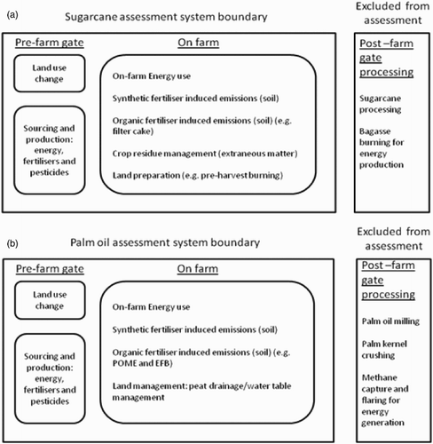
This study focuses on GHG assessment up to the harvesting of the crop (farm gate); that is, it covers GHG emissions from agricultural production and the associated inputs (e.g. fertilizer and pesticide production). It excludes any subsequent steps such as drying, storage, processing and milling. Also omitted are any embedded emissions associated with infrastructure or capital machinery (BSI, 2011); emissions from indirect land use change (iLUC); livestock-induced emissions; or those associated with particular management practices such as rotational cropping or the non-energy impacts of tillage on soil emissions, many of which remain uncertain, complex or are not yet modelled by the tools (Al-Kaisi & Yin, 2005; Melillo et al., 2009; Plevin, O'Hare, Jones, Torn, & Gibbs, 2010; Searchinger et al., 2008). Figure 1(a) and 1(b) shows simplified schematics of the GHG emission sources included in the assessment of the sugarcane and palm oil systems in this study.

Figure 1. Schematics of the GHG emission sources included and excluded from this study assessment for (a) sugarcane, and for (b) palm oil systems.

3.1. Assessment of key GHG drivers

Table 2 provides an overview of the sources of GHG emission assessed by each calculator, showing which GHG emission sources are in and out of scope of the three calculators. The more detailed comparative analysis focused on three major drivers of the GHG footprint of the crops: agrochemical inputs including organic materials, energy use and LU and LUC. They were selected because they represent almost the entire crop-based agricultural GHG footprint (Hillier et al., 2009; Roches et al., 2010; Smith et al., 2007). They are briefly described below.

Table 2. Emission sources considered by the three GHG calculators within the agricultural boundary.^a

GHG emission source^a,^b	Tool
	CFT	Bonsucro	PalmGHG
Fertilizer production (CO2)	Y	Y	Y
Transport of fertilizers to farm (CO2)	Y	Y	Y
(Direct fertilizer emissions) soil N2O emissions from fertilizer application	Y	Y	Y
Indirect N2O from soils from fertilizer application	Y	Y	Y
Pesticide production (includes herbicides, fungicides, insecticides, etc.)	Y	Y	N
Infrastructure (CO2)	N	N	N
Fossil fuel (CO2)	Y	Y	Y
Electricity (CO2)	Y	Y	N (considered in the mill phase only)
Renewable energy generation	Y	N	Y
Crop/mill residues (N2O)	Y	Y	Y
Enteric CH4	Y	NR	NR
Manure CH4	Y	NR	NR
Biomass burning	Y	Y	N
Change in soil C stock from direct LUC	Y	Y	Y (C- and N-related emissions due to peat oxidation; not included for mineral soils)
Change in biomass C stock from direct LUC (sequestration in above and below ground biomass)	Y	Y	Y
Indirect LUC	N	N	N
Peat soils (N2O, CO2)	N	N	Y
Rice (CH4)	Y	NR	NR
Soil C changes due to management changes (tillage, composts, etc.)	Y	N	N
Transport of workers/materials on farm	Y	N	Y (included in total fuel use)
Co-product emissions^c	Y (user-specified co-products)	Y (ethanol, molasses, and sugar)	Y (CPO, PK, and PKO)
Allocation options	None specified as default, user-defined allocation. (economic allocation can be used for co-products)	GHG emissions allocated to sugar and ethanol on an energy basis (57% to sugar, 43% to ethanol) (physical allocation)	Mass (allocation between CPO and PK and between PKO and PKE); system expansion for energy co-products (surplus electricity; PK Shells sold to industrial furnaces)
		Energy inputs allocated to molasses by economic allocation
GHGs considered	CO2, N2O, and CH4	CO2, N2O, and CH4	CO2, N2O, and CH4

^aY, Yes it is included; N, No it is not included; NR, it is not relevant to the crop-specific system and is therefore not included.

^bOther emission sources from processing may be included in the calculator but are not demonstrated in the scope of this assessment.

^cCo-products within and outside of the agricultural boundary, that is, those resulting from the milling of the raw agricultural material, are also indicated here.

3.1.1. GHG driver 1: agrochemical inputs (including organic inputs)

Agrochemical inputs comprise all soil or crop enhancers; fertilizers, both synthetic and organic; pesticides including insecticides, herbicides and fungicides; and crop residues that are either left on the field or returned to the field following processing. In sugarcane cultivation, the inputs include mineral fertilizers, pesticides and crop residues including extraneous matter (EM) which is all the other plant materials left on or returned to the field following harvesting; filter cake (rich in phosphorus); mud; and vinasse (high in potassium). In palm oil production, they include mineral fertilizers and pesticides as well as organic inputs; the empty fruit bunches (EFB) that are returned to the field from the mill after fruit extraction; and palm oil mill effluent (POME), an organic waste material generated from palm oil processing at approximately 0.5–0.75 tonnes for every tonne of fresh fruit bunch (FFB) (Yacob, Hassan, Shirai, Wakisaka, & Subash, 2005). In most agricultural systems, mineral fertilizers are a significant contributor to the overall GHG footprint (Hillier et al., 2009; Johnson, Franzluebbers, Weyers, & Reicosky, 2007). Emissions arise from the high energy demands involved in their production [particularly nitrogen (N) based fertilizers derived from the Haber process]; their transportation, often over large distances, from the source to the farm; and most importantly, nitrous oxide (N₂O) emissions associated with the use of N fertilizers. N₂O emissions occur, as a consequence of the biophysical interactions and microbial processes in the soil, both directly at the time of application, and indirectly, after transport of Nr (reactive N compounds) into ground and surface waters through leaching and surface runoff or it is emitted as ammonia (NH₃) or nitrogen oxides (NO _x ) that are deposited later and elsewhere (IPCC, 2006b). On mineral soils, N₂O emissions from fertilizer use in palm oil cultivation are second only to LUC impacts (not including methane production from POME at the mill stage) (Chase & Henson, 2010) and are also an important contributor in sugarcane production (Rein, 2010).

Other inputs include lime, often applied as a soil enhancer or stabilizer. Lime application emissions are very uncertain (Graboski, 2002) and may even result in an uptake of CO₂ depending on soil conditions and application of other fertilizers (West & McBride, 2005). Emissions from pesticides occur during their production and, in many agricultural systems, afford only a small contribution to the overall GHG footprint due to very limited amounts of active substances applied compared to fertilizer inputs (Hillier et al., 2009). For agricultural inputs, the key parameters that will influence the calculators' results are, therefore, the data sources and assumptions describing fertilizer production and the models applied for N₂O emissions. Finally, the fuel used to transport fertilizers may also have a significant impact, particularly for some inputs that may have very small production emissions (e.g. organic inputs) and depending on the distance travelled and mode of transport. This is addressed under the following GHG driver.

3.1.2. GHG driver 2: energy

Energy is required for transport of materials (agrochemical inputs) and workers to and around the farm, for the general operation of site infrastructure, as well as for other farm operations such as irrigation and land clearing and preparation, for example, tillage, cultivation and harvesting operations. Energy may also be required for the creation and maintenance of access roads, farm drains and on-site storage units. The type of energy source(s) used on a farm site depends upon the context, location and level of mechanization and utilization of farm machinery. The primary fuel used in many Indonesian palm oil and Brazilian sugarcane systems is diesel fuel, used in transportation and machine operations. Grid electricity is also utilized for infrastructure functions and irrigation, for example, and country- or regional-specific energy mixes will determine the associated GHG burden.

3.1.3. GHG driver 3: LU and LUC

LUC involves the conversion of one LU type to another, for example, forest to arable land. It can be a significant source of GHG emissions and may dominate the GHG footprint of production systems due to substantial changes in carbon stocks (Cederberg, Persson, Neovius, Molander, & Clift, 2011; Fargione, Hill, Tilman, Polasky, & Hawthorne, 2008; Searchinger et al., 2008). This is particularly true in tropical areas where deforestation occurs, notably to make way for arable cropping or monoculture plantations such as sugarcane and palm oil (Reijnders & Huijbregts, 2008; Wicke, Dornburg, Junginger, & Faaij, 2008). Emissions due to LUC remain a topic of scientific debate due to several associated uncertainties, thus methodologies employed to calculate it can vary. Estimates are commonly, but not always, based upon IPCC LUC definitions and default factors (IPCC, 2006a). Differences in the consideration and treatment of various carbon stocks including; biomass, both above and below-ground; dead organic matter contained in dead wood and leaf litter; soil organic matter (SOM) contents including high carbon stock soils such as peat soil; as well as the amortization period modelled, can influence the estimates for GHG emissions from LUC (see, e.g. Flynn et al., 2012). Moreover, despite some agreements on the accounting of provisional biogenic carbon storage notably in perennial crops (BSI, 2011; IPCC, 2006a), the debate is still ongoing.

LU includes land preparation through tree felling and chipping or slash and burning, a practice common in sugarcane cultivation ahead of the crop harvest. In this process, the crop is set alight to burn the stalks and dry leaves and to remove any potential hazards in the field (e.g. snakes) for ease of harvest (mostly manual). The combustion results in considerable GHG emissions (De Figueiredo & La Scala, 2011) and so should be reflected in GHG calculations.

Emissions from peat soils are particularly important for palm oil production due to the prevalence of peat in areas where palm oil is grown (peat lands in Southeast Asia represent 57% of the tropical peat area and 77% of the tropical peat carbon pool, of which a large proportion is located in Indonesia and Malaysia, the two top palm oil producing countries (Bessou et al., 2014; Page, Rieley, & Banks, 2011)). Emissions arise from the preparation of the peat from clearing the land and draining the soil, and the continuing emissions resulting from cultivation on peat, that is, from oxidative peat decomposition (Fargione et al., 2008; Germer & Sauerborn, 2007). The scale of the emissions is influenced by the management practices of the land and of the water table, specifically the depth of the water table and the aerobic layer (Moore & Knowles, 1989).

Tables 3–5 present the detail of these GHG driver assessments including some of the default values used in calculations.

Table 3. GHG driver 1: agricultural inputs.

	CFT	Bonsucro	PalmGHG
General approach	CFT combines several empirical models for GHG emissions from agricultural inputs including a fertilizer model based on over 800 data sets (Bouwman et al., 2002), with IPCC tier 1 inventory methods and EFs	The calculation approach is similar to and adapted from the EBAMM model (Farrell et al., 2006), which itself is similar to the GREET model (Wang et al., 2008), modified for sugarcane. The calculator uses IPCC EFs	PalmGHG is based on an earlier model, GWAPP developed by Chase and Henson (2010). It is based on a life-cycle approach specific to global warming impacts. The tool uses both literature data sources and IPCC EFs, combined with oil palm growth models to simulate C sequestration by the crop
Fertilizer production (kg CO2e/kg)	Fertilizer production emissions are specified for a range of fertilizer types (35 fertilizers modelled). Four options are specified for fertilizer production technology used: current tech, new tech, old tech, and older tech Key fertilizers modelled: (kg CO2e/kg)Limestone: 0.006Ammonium nitrate (35% N): 3.042Muriate of potash (MOP) (60% K2O): 0.265Urea (46.4% N) – 2.551Ref(s): Ecoinvent (2002, 2007) and Kongshaug (1998)	Production of N fertilizer is specified, and production and transportation of limeKey fertilizers modelled: (kg CO2e/kg)N fertilizer production: 3.99P fertilizer production: 0.714K fertilizer production: 1.61Lime production and transportation: 0.065Ref(s): Bonsucro production standard appendix 3 (Bonsucro, 2011) and in (Macedo et al., 2008; IPCC, 2006a)	Fertilizer production emissions are specified for nine synthetic fertilizersKey fertilizers modelled: (kg CO2e/kg)Ammonium nitrate (34% N) – 2.380Muriate of potash (MOP) (60% K2O) – 0.2Urea (46% N) – 1.34Ref(s): Jenssen and Kongshaug (2003) and Ecoinvent (2010)
Fertilizer application, direct and indirect N2O emissions	Multivariate empirical model of Bouwman et al. (2002) is used to calculate nitrous oxide (N2O) and nitric oxide (NO) emissions associated with fertilizer application. Emissions from fertilizer application differ for different types of fertilizers applied. Option for user to define own fertilizer blend using a base fertilizerRef(s): Bouwman et al. (2002) and FAO/IFA (2001) (for ammonia)	Fertilizer application emissions differentiated between N, P, K2O and lime with specified EFs for per kg N applied: 6.2 kg CO2e/kg N	Direct and indirect fertilizer-induced emissions are calculated according to IPCC tier 1 and are differentiated between nine widely used synthetic fertilizers in palm oil cultivation. Additional fertilizers can be included if the user requiresRef(s): IPCC (2006a), Jenssen and Kongshaug (2003), Ecoinvent (2010), and Chase and Henson (2010)
		Lime: 0.44 kg CO2e/kg lime (assumes all C in lime becomes CO2)Ref.: IPCC (2007)
Crop residues and organic inputs	Able to model:	Models:	Models:
	Compost – as zero emissions or aerated or non-fully aerated productionSlurry – from livestock typesStrawResidue N content dependent on crop type under assessmentSugarcane (Millet): 0%Palm oil (tree crop): 0.0123%Various residue treatment options modelledRef(s): IPCC (2006a) and Smith et al. (1997)	Cane residue left in field post burning: N content 0.5%Filter cake: N content 12.5%Vinasse: may be applied as a fertilizerAssumed 1.225% of N in the residue is converted to N in N2ORef.: Macedo et al. (2008)	EFB – 0.22 t/t FFB, N content 0.32%*POME – 0.5 t/t FFB, N content 0.045%**N contents and production rates can be modified by the userRef(s): Yacob et al. (2005) and Singh (1995)
N runoff, leaching rate	30% for moist soils, none for dry	Not specified	30%
	Ref.: IPCC (2006a)		Ref.: IPCC (2006a)
Pesticides	Average emissions factor for all pesticides (based on production emissions)are included per application dose: 20.5 kg CO2e	Insecticide EF: 29.09 kg CO2e/kg Herbicide EF: 25.05 kg CO2e/kgRef.: Macedo et al. (2008)	Not included
	Ref(s): average generated from: Audsley (1997) and Green (1987)
Management inputs	IPCC tier 1 method is used to estimate soil C stock changes and the changes due to management practices are defined by Ogle et al. (2005). They are modelled on an annualized basis and are dependent on several farm characteristics including climate	Not included	Not included
GWP values	N2O: 296	N2O: 298	N2O: 298
	CH4: 25	CH4: 25	CH4: 22.25 (bio-methane, for example, from POME)
	Ref(s): IPCC (2001), IPCC AR4 (2007) and Smith et al. (2007)	Ref(s): IPCC AR4 (2007) and BSI (2008)	Ref(s): IPCC AR4 (2007), Chase and Henson (2010) and Muñoz, Rigarlsford, Canals, and King (2012)

Note: EBAMM, Energy and Resources Group (ERG) Biofuel Analysis Meta-Model.

Table 4. GHG driver 2: Energy.

	CFT	Bonsucro	PalmGHG
General approach and activity data required	Reported on a total annual consumption basis per fuel type used with the option to specify several fuel types. Alternatively/in addition, emissions arising per machine operation for various practices can be calculated based on number of operations, fuel used and other farm characteristics stated	Total annual fuel use per fuel type across all agricultural activities is reported. Electricity used in irrigation is reported separately	Recorded as total fuel consumption (of diesel and petrol) in one year of plantation lifetime. It includes emissions due to field operations that arise from fossil fuel consumed by machinery for transportation and other field operations
Fuel EFs
Gasoline/petrol (kg CO2e/L of fuel)	2.32	2.81	3.12 (Assumed as diesel)
	Ref.: GHG Protocol (2003)	Ref(s): Farrell et al. (2006), Shapouri, Duffield, McAloon, and Wang (2004), Graboski (2002) and Macedo et al. (2008)	Ref.: JRC, EUCAR, and CONCAWE (2011)
Diesel (kg CO2e/L of fuel)	2.68	3.46	3.12
	Ref.: GHG Protocol (2003)	Ref(s): Farrell et al. (2006), Shapouri et al. (2004), Graboski (2002) and Macedo et al. (2008)	Ref.: JRC et al. (2011)
Fuel oil (kg CO2e/MJ)	0.0784 kg CO2e/MJ	0.096 kg CO2e/MJ	Not included
	Ref.: GHG Protocol (2003)	Ref.: Farrell et al. (2006) (EBAMM)
Natural gas (kg CO2e/MJ)	0.0628 kg CO2e/MJ	0.066 kg CO2e/MJ	Not included
	Ref.: GHG Protocol (2003)	Ref.: Farrell et al. (2006) (EBAMM)
Coal (kg CO2e/MJ)	0.0927 kg CO2e/MJ	0.107 kg CO2e/MJ	Not included
	Ref.: GHG Protocol (2003)	Ref.: Farrell et al. (2006) (EBAMM)
Electricity (kg CO2e/MJ)	Country-specific values for kg CO2e/MJ grid electricity are included in the tool	Country-specific values for kg CO2e/MJ grid electricity should be specified. Values stated in Bonsucro production standard	Not included in the agricultural phase
	Value for Brazil: 0.02	Value for Brazil: 0.02
	value for Indonesia: 0.21	Value for Indonesia: 0.22
	Ref.: IEA (2009 figures)	Ref.: RFA (2008)
Renewable electricity sources (kg CO2e/MJ)	Option to include emissions generated from the use of renewable electricity sources:	Not included	Not included
	Hydro: 0.0017
	Wind: 0.033
	Photo-voltaic: 0.01972
	Ref.: Ecoinvent (2007)
Specific machine operation energy consumption	Simplified model for fuel use as a function of machinery operations for basic farm management practices (tilling, harvesting, etc.). for differing soil types and yields	Electricity used in irrigation (including vinasse distribution) is modelled separately using the same EF for electricity	No specific machine operations included
	Ref.: ASABE (2006a, 2006b)	No other specific machine operations included
Energy used in transportation of inputs to farm	Calculated based on quantity transported, distance travelled and mode of transport and vehicle/vessel type. Option for weight of vehicle to be included also	Transport emissions calculated as 0.05 kg CO2e/kg input material transportedRef.: Wang et al. (2008)	Transport of fertilizers from production sites to field are included based on shipping and motor vehicle emissions0.31 kgCO2e/km.t (assumes 2l diesel/km at 20t per trip)Ref.: www.searates.com; Chase and Henson (2010)

Table 5. GHG driver 3: LU and LUC.

	CFT	Bonsucro	PalmGHG
General approach	User specifies broad category of LUC that has occurred, with more specificity if forest land; how long ago the change occurred and the percentage of the total land area converted. If converted from forest the user can state the age of the forest when felled	Emissions from any land use change are calculated outside of the tool using values given in: http://shop.bsigroup.com/upload/Shop/Download/PAS/PAS2050.pdf	Emissions from land clearing by burning are calculated based on user-specified percentage of crop burnt
			Emissions are calculated for land clearing each year and averaged over the full crop cycle. ‘Own crops’ and ‘out-growers’ can be modelled separately, as can emissions arising from mineral soils and peat soils. The user is required to specify how much land area was changed from different previous land use types at planting and the amount of C lost is then amortized over the expected crop cycle
Previous land use types included:	Forest land (several types)	Forest land	On mineral soils:
	Tropical forest	Grassland	Primary forest
	Tropical moist deciduous forest	Crop land	Logged forest
	Tropical dry forest		Coconut
	Tropical shrubland		Rubber
	Tropical mountain system		Cocoa under shade
	Sub-tropical humid forest		Oil palm
	Sub-tropical dry forest		Secondary re-growth
	Sub-tropical steppe		Shrubland
	Sub-tropical mountain system		Food crops
	Temperate oceanic forest		Grassland
	Temperate continental forest
	Temperate mountain system		On peat soils:
	Boreal coniferous forest		Logged forest
	Boreal tundra forest		Food crops
	Boreal mountain system		Secondary re-growth
	Grassland		Oil palm
	Arable
Land use carbon stocks	PAS 2050 default values used	PAS 2050 default values used	Defined in Agus et al. (2012)
Peat soil emissions	Not included specifically (soil characteristics can be modified to be more representative of peat soil)	Not included	Emissions from oxidation of organic carbon and associated N2O emissions from peat cultivation based on water table depth and management
			Calculation: 0.91 (t CO2e/ha/yr) × cm drainage depth
			Ref.: Hooijer et al. (2010)
Burning/combustion (pre- or post-crop harvesting)	Not included specifically (however can be modelled through specifying burning as the treatment of crop residue)	Emissions from cane burning are based on IPCC EFs for burning biomass (0.07 kg N2O/t dry matter and 2.7 kg CH4/t dry matter)	Not included
		Ref.: IPCC (2006a)
C stock changes related to management practices (e.g. tillage, composting, planting preparation etc.)	IPCC tier 1 method employed for estimating soil C stock changes. Changes determined by Ogle et al. (2005) for a period of 20 years.	Not included. (changes in C content of soils other than those from direct land use change are excluded)	Not included
LULUC-induced soil C stocks	Defined by Ogle et al. (2005)	Not included	Not included (for mineral soils)
Amortization	20 years	Not included within the tool	Default is 25 years (but can be modified by user)
	Ref(s): IPCC (2006a) and BSI (2011)		Ref(s): Chase and Henson (2010)
Crop sequestration in assessment crop	Not included (unless modelled specifically under crop sequestration tab)	Not included (biogenic sources of carbon are excluded except those resulting from direct LUC)	Direct measurements preferable otherwise modelled data are used based on Southeast Asian conditions to produce annual values for standing biomass (above and below-ground), ground cover, frond piles and other plantation litter
Carbon content of biomass	50%	Not included	45 or 46%
			Ref.: Chase et al. (2012)
Sensitivities	Unable to model different land use change scenarios in the same spreadsheet	NA	Differences in crop ages throughout the plantation are captured
Underlying models incorporated	Several data sets and allometric growth models from IPCC (2006a) to model carbon storage in tree crop systems	Not included	OPRODSIM and OPCABSIM (vigorous growth for own crops and average growth for out-growers
			Ref(s): Henson (2005, 2009)

3.2. Output-based comparison

The two crop systems were studied with their respective crop-specific calculator and the general CFT: sugarcane production in Brazil (Bonsucro calculator) and palm oil cultivation in Indonesia (PalmGHG calculator). The farming data sets for each crop were provided by the commodity roundtables (M. Chin, personal communication, June 8, 2012; N. Viart, personal communication, November 10, 2012) and are summarized in Tables 6 and 7. The data sets are representative of typical farms for the systems compared, based on expert judgement, however, they are not intended to represent the whole of the sectors and so the data and results should not be used to compare different crop production emissions outside of this study. Tables 6 and 7 present the ‘base case’ data used for the comparison unless otherwise specified when modelling different scenarios or user options available in the tools.

Table 6. Input data for sugarcane assessment (base case).

Information category	Input	Data entry/quantity	Units	Source/reference	Tool(s) using the data
General information	Crop type	Millet		Closest representation to sugarcane as an option in the CFT	CFT
	Yield	1,700,372	Ha	Specified by N. Viart (personal communication, November 10, 2012)	Both
	Production area	27,231	Tonnes		Both
	Climate	Tropical: annual average temperature: 18	°C		CFT
Soil properties	Soil type	Medium			CFT
	SOM content	1.72 < SOM≤5.16			CFT
	Soil moisture	Dry			CFT
	Soil drainage	Good			CFT
	Soil pH	≤5.5	pH		CFT
Fertilizers applied	Nitrogen (N) [as urea in CFT]	65.7	kg/ha		Both
	Phosphorus (P) [as triple super phosphate in CFT]	39.5	kg/ha		Both
	Potassium (K) [as potassium sulphate in CFT]	65.9	kg/ha		Both
	Lime [as limestone in CFT]	236.7	kg/ha		Both
Fertilizer related information	Fertilizer application method	Incorporate			CFT
	Emissions inhibitors in fertilizers	None			CFT
	Fertilizer production technology	Current technology			CFT
Organic inputs	Filter cake [as zero compost emissions in CFT]	3400	kg/ha		Both
Pesticide application	Herbicide	3.96	kg/ha		Bonsucro
	Insecticide	0.71	kg/ha		Bonsucro
	Number of applications	4	Applicat-ions/yr	Specified by N. Viart (personal communication, September 12, 2013)	CFT
Transport of inputs	Quantity transported	11,104	tonnes	Authors’ assumptions
	Mode of transport/distance transported	Heavy goods vehicle/200	Vehicle type/km
Energy use	Gasoline	100	l/ha	Authors’ assumptions	Both
	Diesel	7,212,659 (264.87 litres per ha)	Litres per year	Specified by N. Viart (personal communication, November 10, 2012)	Both
	Natural gas	50	kWh/ha	Authors’ assumptions	Both
	Electricity	90	kWh/ha	Authors’ assumptions	Both
Crop residue	EM quantity	3126	Kg/ha	Specified by N. Viart (personal communication, November 10, 2012)	Both
	Treatment	Left on field; incorporated or mulch			CFT
Land clearing	Sugarcane burnt	48.05	% of crop		Bonsucro
		30	t cane/ha		Both
Land use change Scenarios modelled	Forest to arable cropland	100% land conversion	%	Authors’ assumptions for comparison purposes only	Both
	Forest to perennial cropland				Bonsucro
	Forest to grassland				CFT

Table 7. Input data for palm oil assessment (base case).

Information category	Input	Data entry/quantity	Units	Source/reference	Tool(s) used in
General information	Crop type	Tree crop		Closest representation to oil palm as an option in the CFT	CFT
	Yield	195,333	Tonnes	Specified by M. Chin (personal communication, June 8, 2012)	Both
	Production area	6822	ha		Both
	Climate	Tropical: annual average of 18	˚C		CFT
Mineral soil properties	Soil type	Fine			CFT
		Mineral soil			PalmGHG
	SOM content	1.72 < SOM ≤5.16	%		CFT
	Soil moisture	Moist			CFT
	Soil drainage	Good			CFT
	Soil pH	≤ 5.5	pH		CFT
Peat soil properties	Soil type	Fine soil			CFT
		Peat soil			PalmGHG
	SOM content	10.32 < SOM	%		CFT
	Soil moisture	Moist			CFT
	Soil drainage	Poor			CFT
	Soil pH	≤5.5	pH		CFT
	Water table	Actively managed	Y/N	(defaults: not actively managed = 80; actively managed = 60) RSPO PLWG (2012)	PalmGHG
		Depth of water table	Cm
Fertilizers applied	Ammonium nitrate	80	kg/ha	Specified by M. Chin (personal communication, June 8, 2012)	Both
	Urea	20	kg/ha		Both
	Kierserite	70	kg/ha		Both
	Murate of Potash	200	kg/ha		Both
	Triple super phosphate	70	kg/ha		Both
	Ammonium sulphate	80	kg/ha		Both
Organic inputs	FFB	0.22	t/t FFB		Both
	POME	0.5	t/t FFB		Both
Pesticide application	Number of applications	3	Applications per year	I. Henson, personal communication (May 2013)	CFT
Transport of inputs	Quantity transported	3525	tonnes	Authors’ assumptions	Both
	Mode of transport/distance transported	Road, light goods vehicle/50	Vehicle type/km
	Mode of transport/distance transported	Ship/4000	Vehicle type/km
Energy use	Diesel	388,333	Litres per year	Specified by M. Chin (personal communication, June 8, 2012)	Both
		56.924	Litres per ha
Crop residue	Frond piles and plantation litter (residue)	8.54	t biomass/ha	I. Henson, personal communication (May 2013)	CFT
Land use change Scenarios modelled	Forest to plantation	100% land conversion	%	Authors’ assumptions for comparison purposes only	PalmGHG
	Forest to arable cropland				CFT
	Forest to grassland				CFT

Direct comparison of the tools is challenging due to differences in data input requirements and formats. In a few aspects, minor amendments to formulae in the tools were made to render the calculations more directly comparable (e.g. amortization period for palm oil). Table 8 lists the edits made to harmonize and align the calculations of the tools. Otherwise, results were generated without editing the underlying data or calculation algorithms, in order to compare results from the tools in their generally available forms.

Table 8. Issues faced and assumptions made during the GHG assessments with the calculators.

GHG source (crop system)	Issue	Tool	Assumption and justification
Land clearing (sugarcane)	No specific data input option for land clearing by combustion	CFT	Modelled under residue management functionality, ‘burned’. Residue quantity equated to the amount of dry matter burnt per hectare
Pesticides (sugarcane)	Quantity of different pesticide types present for Bonsucro. Unknown number of applications per year for CFT data entry	CFT	Assumed four applications including one application pre-planting (N. Viart, personal communication, September 12, 2013)
Residual EM (sugarcane)	Quantity of EM is calculated within Bonsucro but unavailable for CFT. A calculation was performed external to the tools:	CFT	Estimated 3125.75 kg/ha residue left in field/incorporated or used as mulch
	= 3126 kg/ha
Transport of fertilizers (sugarcane)	Information on; distance of fertilizer production to farm; mode and type of vehicle; and if (for road) it returned empty or not, unavailable	CFT	Assumptions made were^a:
			Distance: 200 kmMode: roadVehicle: heavy goods vehicleReturn: returning empty
Fertilizer production technology (sugarcane; palm oil)	Unknown state of technology	CFT	Assumed current technology (default option in CFT)
Amortization of carbon stock biomass loss (sugarcane; palm oil)	GHG emissions for biomass loss are accounted for in the year they are lost and not amortized (this is based on IPCC accounting for national inventories	CFT	A 20-year amortization period was applied to the biomass loss GHG emissions for sugarcane and 20- and 25-year amortisation periods were used for palm oil data
EFB and POME (palm Oil)	No equal or closely equivalent fertilizers included in the CFT	CFT	Modelled under zero emissions compost (1% N) and cattle slurry (0.26% N) as the closest fertilizers with a low N content to reflect that of EFB and POME
Farm situation (palm oil)	Modelling different farm properties	PalmGHG	Assumed to be own crop only (no out-growers modelled), mineral soils only (no peat modelled)
Three-year rolling average (palm oil)	PalmGHG requires three years of data input and uses the average value to calculate the GHG footprint	PalmGHG	The same data set was entered for each of the three years to ‘force’ the tool to use the one-year data value as the average

^aAuthors' assumptions.

Results from the different calculators are reported here on a per land area basis (kg CO₂e per ha cultivated) across a number of GHG emission sources including fertilizer production, transport and application, emissions from organic inputs, and from pesticide production and emissions associated with energy use. LUC results are presented separately based on some modelled scenarios summarized in Tables 6 and 7. The analysis indicates where and how the tools differ when using the same input data due to differences in system boundaries, calculation methodologies or EFs.

4. Output-based results

4.1. Sugarcane results (CFT vs. Bonsucro)

Figure 2 shows the results for each GHG emission source for Bonsucro and the CFT and highlights where the differences occur. The differences in results per GHG emission source range from a 12% difference for emissions for lime production and application up to 42% for mineral fertilizer related emissions with Bonsucro generating larger values for each source apart from EM residue management. Despite the larger GHG emissions reported by Bonsucro per hotspot, the total GHG footprint for sugarcane cultivation from the tools was 2407 kgCO₂e/ha for Bonsucro and 2229 kgCO₂e/ha² for the CFT, a difference of 8% (LUC excluded); considerably less than the difference between several individual emission sources. This is because the final GHG footprint from the CFT includes ‘background’ direct and indirect N₂O emissions which arise from the soil and vary depending on the soil and climate conditions and include the decomposition of plant material in the soil which are not attributed to one particular GHG emission source (Bouwman, Boumans, & Batjes, 2002).

Figure 2. GHG emission hotspot results for sugarcane production generated by Bonsucro and the CFT (kg CO₂e/ha).

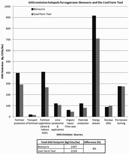
4.1.1. Sugarcane and GHG emissions from agricultural inputs

Fertilizer production emissions for Bonsucro were 30% greater than those produced by the CFT, due primarily to differences in EFs and specifically the higher emissions factor for N-fertilizer production used in Bonsucro. The fertilizer production emission values used in Bonsucro are taken from the EBAMM model which is itself based on the GREET life-cycle model for transport fuels which represent US values (Macedo et al., 2008; Wang et al., 2008; GREET 1.6). In comparison, the CFT contains a range of fertilizers of different nutrient blends that the user can select from and the production emissions are largely based on European fertilizer manufacture data (EFMA and Ecoinvent) which is among the world's most efficient and in some cases is close to the technological limit of efficiency (Brentrup & Palliere, 2008). The efficiency in technology alone, does not explain why the difference in emissions is so pronounced without greater transparency on where the numbers have been derived from. There are often high levels of discrepancy and uncertainty in the way databases on fertilizer production are built up (C. Bessou, personal communication, June 16, 2014). Several fertilizer production data sets are included within the CFT that contain different production factors; in this assessment, the default data set was used. The implications of using alternative data sets are explored later in the palm oil assessment.

Both tools model lime inputs as limestone and use the same tier 1 IPCC factor that assumes that all the carbon (C) is released as carbon dioxide (CO₂). The emissions profile for lime from Bonsucro, however, was 12% higher than the CFT, due to differences in the modelling of lime production emissions; US data are used in Bonsucro compared to European production data in the CFT.

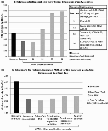
To calculate field-based fertilizer emissions, Bonsucro requires the user to describe fertilizer application based on the quantity of nutrient (N) applied and GHG emissions are calculated based on one-specific GHG EF per unit of N applied (6.2 kg CO₂e/kg N, taken from (IPCC, 2006a)). In contrast, the CFT calculates the direct and indirect GHG emissions using different EFs for each fertilizer blend and integrates the various degradation and transfer processes for Nr-compounds (nitrification, denitrification, volatilization, leaching and runoff) (Bouwman et al., 2002). For the comparison, urea was selected in the CFT to represent the N input. In Bonsucro, the soil properties are fixed (and not specified), whereas in the CFT, the user must enter a number of different soil parameters. Figure 3(a) shows the effect on the GHG emissions of varying the soil properties (derived from (Bouwman et al., 2002)) (soil type; SOM; soil moisture; drainage; and pH) through a number of different soil property scenarios (S) in the CFT (S1–S4). These soil property scenarios modelled in the CFT are compared to the emission estimate from Bonsucro for the same amount of urea (N) applied. A difference of 99% between the base case soil properties (as per Table 6) and scenario 4 (S4), highlights the influence of different soil parameters on the GHG emissions. It is clear to see from Figure 3(a) that the base case is closer to the lower end of the possible range shown (S1), whereas the output for Bonsucro is larger than this, and closer to S2. Figure 3(b) shows the effect on the GHG emissions of various fertilizer application methods that can be selected in the CFT. This effect is clearly less significant than that of varying soil properties.

Figure 3. (a) GHG emissions from urea (N) fertilizer application in Bonsucro and various soil property scenarios in the CFT (S1–S4) and (b) fertilizer-induced GHG emissions for Bonsucro when using different fertilizer application methods in the CFT.

The differences in the emissions for crop residue management (Figure 2) are primarily due to a different N-content assumed for the residue³ in the CFT, 0.7% N (IPCC, 2006b) compared to the more specific N content of sugarcane EM, 0.5% N (Macedo et al., 2008) in Bonsucro.

4.1.2. Sugarcane and GHG emissions from energy use

GHG emissions from diesel use are presented in Figure 2; however, both Bonsucro and CFT enable the user to model emissions for other types of energy used; gasoline (petrol), natural gas and electricity. Table 9 presents the GHG emission outputs generated by the two tools for each energy type, the corresponding EF and the percentage difference between the tools in each case. The energy quantities modelled here were based on representative amounts for a Brazilian sugarcane system where available (Macedo et al., 2008; Rein, 2010), otherwise authors' assumptions were used. The differences in GHG emission outputs for diesel, gasoline and electricity generated by the two tools correspond directly to the differences in the EFs used whereas the results for natural gas differ due to different EFs and the inclusion of an energy demand factor in Bonsucro used to convert direct energy to primary energy (Macedo et al., 2008).

Table 9. GHG emission outputs and EFs for various fuel types included in Bonsucro and the cool farm tool.

Energy type and Input	Factor	GHG calculator		Percentage difference (%)
	Output	Bonsucro	CFT
Diesel (7,212,659 litres per year)^a	EF (kg CO2e/MJ)	3.46	2.68	25.4
	GHG output (kg CO2e/ha)	916	709.9	25.4
Gasoline (100 litres/ha)^b	EF (kg CO2e/l fuel)	2.81	2.32	19.1
	GHG output (kg CO2e/ha)	281.16	232	19.2
Electricity (90 kWh/ha)^c	EF (kg CO2e/MJ)	0.022	0.018	21.3
	GHG output (kg CO2e/ha)	7.13	5.75	21.3
Natural Gas (50 kWh/ha)^b	EF (kg CO2e/MJ)	0.0662	0.0628	5.2
	GHG output (kg CO2e/ha)	10.64	11.3	6
	Energy demand factor	1.12	N/A	N/A

^aBase case data set (from Table 2).

^bAuthors’ assumed quantity.

^cRein (2010).

4.1.3. Sugarcane and GHG emissions from LU and LUC

Both tools use the same biomass burning factors from IPCC (IPCC, 2006a); therefore, the GHG emission outputs for pre-harvest combustion are comparable (Figure 2), despite differences in the requirements of users to input representative quantities of crop burnt.

The two tools calculate emissions from LUC differently. Bonsucro requires direct entry of the LUC GHG emissions calculated by the user using the IPCC default values specified in PAS 2050 (BSI, 2011) relevant to the country being modelled. The CFT requires the user to choose the type of LUC from a pre-defined list (involving forest land, grassland and arable cropland (perennial cropland is not included)); when the change occurred (up to a maximum of 20 years); and the type of forest replaced (if any). Figure 4 shows the sensitivity of the LUC results to the varying specificity of the two tools in terms of land types and associated carbon stocks; note that the values presented in the figure are ca. 2 orders of magnitude higher than the contributions shown for fertilizer emissions in Figure 2. Table 10 compares the results for conversion from forest to arable cropland by both Bonsucro and CFT, given different specified soil parameters in the CFT, where results range from a 2% to a 16% difference. These differences are driven by the changes in soil carbon stocks and demonstrate some important differences between the tools, particularly given the significance of LUC emissions to the overall footprint.

Figure 4. GHG emissions from various land use change (LUC) scenarios for sugarcane modelled in Bonsucro and the cool farm tool.

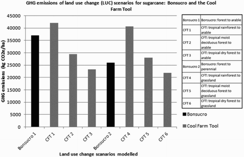
Table 10. GHG emissions for LUC from forest to arable given different soil properties in the cool farm tool.

Tool scenario	LUC type specified	Soil property amendment (from base case, Table 2)	GHG output (kg CO2e/ha)
Bonsucro 1	Forest to arable	–	37,000
CFT 7	Tropical rainforest to arable	Soil type: fine	37,803
CFT 8	Tropical rainforest to arable	Soil type: coarse	43,472
CFT 9	Tropical rainforest to arable	Lower SOM: ≤1.72	39,892
CFT 10	Tropical rainforest to arable	Higher pH: >8.5	37,746

4.2. Palm oil results (CFT vs. PalmGHG)

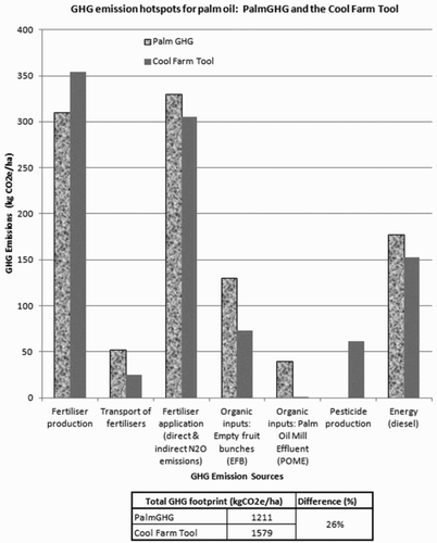
The results for palm oil production modelled with PalmGHG and the CFT across different GHG emission sources are presented in Figure 5. PalmGHG generates results higher than the CFT for all emission sources except for those from pesticide production (which are omitted entirely from PalmGHG) and those associated with mineral fertilizer production. Some results differ based directly on the different GHG EFs used, for example, diesel energy use, whereas others are due to more substantive differences between modelling approaches and different background data and calculations. The CFT also includes a large reported quantity of background emissions in the overall calculation, as described earlier, leading to a higher overall footprint reported by the CFT, a difference of 26% overall, LUC excluded.

Figure 5. GHG emission outputs for palm oil generated by PalmGHG and the CFT across different GHG hotspots (kg CO₂e/ha).

4.2.1. Palm oil and GHG emissions from agrochemical (and organic) inputs

Nine mineral fertilizers widely used in palm oil cultivation are specified in PalmGHG, of which six were modelled in the palm oil data set and are also built into the CFT in some form. (Where an exact match was absent, the closest equivalent fertilizer, with regard to nutrient content, was modelled).

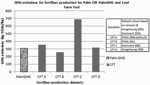
In the modelled systems, fertilizer production emissions differed by 13% due to the difference in EFs/data sources. The CFT contains several fertilizer production data sets and Figure 6 shows how sensitive the results are to the data set selected; 75% difference if using Ecoinvent (2007) in the CFT or just 1.5% difference when using Kongshaug (1998), an updated version of which is used in PalmGHG (Jenssen & Kongshaug, 2003).

Figure 6. GHG emission outputs for fertilizer production for a palm oil production system generated by PalmGHG and the CFT based on different data sets within the tools.

GHG emissions from mineral fertilizer application and those associated with organic inputs; EFB and POME that are returned from the mill to the field; are 8%, 56% and 192% higher, respectively, when calculated with PalmGHG. Results are driven by the respective N-contents of the fertilizers which determine field N₂O emissions. The differences in results reflect different underlying data sources or EFs used in the two tools and also the limitations of the CFT to model organic inputs specific to palm oil production as adequately as PalmGHG. EFB (0.32% N) and POME (0.045% N) (Singh, 1995) were modelled in the CFT based on ‘zero emissions compost 1% N’ and as ‘cattle slurry 0.26% N’, respectively, to reflect the composition of these organic inputs as proxies in the CFT in its available form.

4.2.2. PalmGHG and energy associated GHG emissions

PalmGHG produced results 15% higher than the CFT, which is directly associated in the difference of the GHG EFs used for diesel (see Table 4).

4.2.3. Palm oil and GHG emissions from LUC

PalmGHG includes a comprehensive modelling of LUC over the first crop cycle which is generally between 20 and 27 years (Chase & Henson, 2010; Chase et al., 2012) post-land conversion. PalmGHG enables the user to specify LUC to palm oil plantation from several previous LU types including; primary forest; logged forest; grassland; cocoa and coconut plantations; arable food cropland; or from secondary re-growth, each with a specified carbon stock (Agus et al., 2012). The tool allows the user to specify areas of land cleared from each LU type that might have occurred at different times during the development of the palm oil plantation. The CFT provides less specificity and adopts a simpler approach, as described earlier, to model any significant GHG emissions from a narrow range of LUC categories that may have occurred within the farming system over 20 years, as recommended by IPCC (2006a). The CFT does not include C stock values for perennial plantations, making direct comparison difficult. However to compare the tools, some standardized LUC scenarios were modelled, shown in Figure 7(a), using ‘arable land’ and ‘grassland’ LU types as proxies. The differences in the GHG results are driven by two key aspects of the tools approaches and data sources for LUC. First, there are different carbon stock values incorporated for the LU classifications; PalmGHG includes carbon stocks in below and above ground biomass taken from a variety of sources (Chase et al., 2012), whilst the CFT uses values from tier 1 IPCC (2006a) data and soil carbon stock changes from Ogle, Breidt, and Paustian (2005). The ‘tropical rain forest’ LU category in the CFT was modelled as equivalent to the ‘primary forest’ category in PalmGHG (to represent the higher C stock LUs present in the tools, although these values differ; 350 t C/ha in CFT compared to 225 t C/ha in PalmGHG). The second key difference is the amortization period and approach used (the CFT was adapted to facilitate amortization of above ground biomass losses (see Table 8)). Figure 7(a) shows the GHG emissions from LUC for PalmGHG and CFT for different amortization periods, 20 years and 25 years and for conversion to both arable and grassland modelled in the CFT, highlighting the influence of the amortization period used. There is a difference of 22% in the results from PalmGHG for 20 and 25 years amortization, which, given the importance of LUC as an emission source, can have a significant impact on the overall footprint.

Figure 7. (a) GHG outputs for LUC scenarios for palm oil as modelled in PalmGHG and the CFT (kg CO₂e/ha) and (b) GHG outputs for LUC scenarios for palm oil on peat soils as modelled in PalmGHG and the CFT (kg CO₂e/ha).

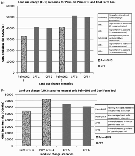
Another important LU factor for palm oil is cultivation on peat soils. PalmGHG has provisions to model emissions from peat under managed and unmanaged scenarios (in relation to the depth of the water table). There is no special provision for peat soil in the CFT but a ‘pseudo-peat’ soil can be modelled through specification of representative (high C content) soil properties (described in Table 7) although the management aspects in relation to the water table (and thus the extent of peat oxidation) cannot be modelled. Modelling peat soil in the CFT by way of the soil properties will influence the N₂O emissions however will not add to the CO₂ emissions (which can be more significant, particularly in regard to different management actions, i.e. peat oxidation) as it does in PalmGHG which is based upon IPCC values and is calculated using the equation from Hooijer et al. (2010). Figure 7(b) shows the results for managed and unmanaged water tables for peat soils in PalmGHG and the equivalent representation of peat soil in CFT on the two LUC scenarios, tropical rainforest converted to arable and to grassland. The GHG emissions are substantial and Figure 7(b) indicates the range of results that may be generated.

5. Discussion

5.1. Comparison of the calculators

Findings of the study first show that, whilst the tools are in broad agreement, the results can differ by considerable margins. This is due to differences in underlying data sources, varying methodologies and approaches employed in the tools. In some cases, differences between the tools are directly related to the difference in the EFs and data used (e.g. for diesel emissions); in other cases, there are more complicated interactions of different parameters within the tools. This is often the case in the CFT, which being positioned as a general tool, consequently has to incorporate more in-built flexibility to enable several different systems to be modelled effectively. The CFT includes numerous options to model increased site-specificity such as climate conditions (temperature) and soil properties as well as more specific management practices such as fertilizer application methodology or the state of the fertilizer production technology. These parameters have, in some cases, considerable impacts on the GHG results. The crop-specific tools do not provide the same range of user options to define the farm conditions; they appear to inherently include some of these parameters within the tool (e.g. soil type/climate) and therefore provide a level of expertise or detail specific to the crop or system, however, the sources of the underlying assumptions are not always clear (particularly within Bonsucro). Fewer user options can aid tool completion and reduce the data entry burden, however, this introduces some generalities as it loses some specificity and the opportunity to understand for example, how variable the soils are between different systems or the subtle differences between fertilizer application methodologies.

The variability in results between the tools does not imply that they are invalid. The three tools typically incorporate published data sources and standardized approaches or EFs such as those from IPCC, and thus apply ‘best available science’ where possible. More so, the variability in results demonstrates the influence of the choice of background data and the importance of understanding it. This is particularly important for future tool developers or those seeking to use their outputs in a reporting context. Results range from full equivalence when the same data source has been used, for example, GHG emissions for pre-harvest combustion in sugarcane production, by the CFT and Bonsucro; to grossly different in cases where crop-specific factors are incorporated, for example, for POME inputs in palm oil production, by PalmGHG compared to the CFT. Despite some large differences between tools in the results for individual GHG sources, in both assessments there appears to be a ‘smoothing effect’ of aggregating emissions across the entire system, which could be an artefact of the data entry in this particular case.

Second, this paper provides a structured assessment of several of the underlying features and data sources, providing some of the detail necessary to enable improved comparison and interpretation of the results. The tools vary in their degree of transparency. In Bonsucro much of the underlying data used in the calculations are explicitly presented at the data entry stage thus the calculations performed are relatively simplistic, although it is not always documented where the data has been sourced from. In the CFT and PalmGHG, the underlying data are also contained within the tool spreadsheets though these are not always explicit and are often contained in the background of the calculation sheet and the calculation formulas used can be difficult to decipher. This is more pronounced in the CFT due to the greater variety of combinations of different parameters. Furthermore, this assessment highlights the difficulty in direct comparison of the tools due to the different modelling approaches, structures, units and nomenclature used. In some cases, amendments were made to the tools (see Table 8) to make them more comparable. An expert user, however, could manipulate the tools further (given the access rights), to ‘force’ greater consistency and comparability. This could be done by altering background data or algorithms, for example, edit carbon stock values, change EFs, or in the CFT for instance, select in-built default values that are most similar to the other tool, for example, the choice of different fertilizer production data sets. Changes such as these, however, should only be made by an administering body, for example, the certification scheme, and caution must then be taken if comparing results with the ‘same’ generally available version of the tool.

5.2. Implications and future considerations

The tools seek to provide decision-support for farmers, yet the differences in output could have important implications in practice. Although the tools are generally in agreement on the magnitude of the GHG emission source, a farmer may select to focus or invest in different mitigation actions depending on the tool they use. For example, the results from Bonsucro for sugarcane production indicate that more attention should be paid to emissions from fertilizer application than pre-harvest burning activities, whereas the CFT suggested the opposite (that the emissions from burning are more important) (see Figure 2), thus there is a difference of direction between the tools in this instance.

Whilst the use of calculators within certification schemes is still relatively immature or is primarily targeted at assessing continuous improvement (SAN, 2010; Unilever, 2010), results show that differences between the GHG emission results from different calculators are of comparable magnitude to the differences between individual farms. Comparison between farmers cannot therefore be based on the results from different calculators. RSPO require GHG quantification and advocate use of PalmGHG or an ‘equivalent’ calculator, without providing any guidance on what might be considered equivalent. It is demonstrated here that results can differ due to many factors and superficially similar calculators containing the same GHG emission sources cannot be considered equivalent on this basis alone. A greater understanding of the detail behind different calculators is required in order to reconcile and compare results. This and other studies (Colomb et al., 2013; Hennecke et al., 2013; Whittaker et al., 2013) help to build up experience and knowledge surrounding the issues of comparability of agricultural GHG footprint results when generated by different calculators even when using uniform data sets. GHG modelling of agricultural systems is a complex undertaking, yet compatibility of calculators is a challenge that is also faced in other sectors, for example, personal carbon footprinting (Padgett, Steinemann, Clarke, & Vandenbergh, 2008).

As calculators continue to develop, the challenge of keeping up with new and evolving science could add further inconsistencies between them. This could be in the form of improved science for the measurement of particular GHG emission sources; new accepted methodologies for additional emission sources, iLUC, for example; a requirement to model the uncertainty associated with emission estimates; or changes to GHG global warming potentials (GWP) such as the recent update of the methane GWP in AR5 (IPCC, 2013). Given the importance of the background data in driving differences in results, calculators may adopt different scientific developments at different times, thus discrepancies are likely to persist and create additional challenges of version control. Furthermore, with the advent of calculators going ‘online’, there may be the opportunity to introduce greater flexibility and sophistication but may generate trade-offs with an increased potential for user error or reduced transparency in the tool. Conversely, developments in science and new online platforms could lead to calculators converging to utilize similar background models and share approaches to modelling LUC or other impacts.

Although farm-level GHG calculators are currently used at the individual farm level, there is increasing attention on landscape approaches and ‘macro’ level assessments. Several certification schemes, for example, have joined the Committee On Sustainable Agriculture (COSA) which seeks to analyse the impacts of agriculture at a larger scale, particularly those impacts associated with the implementation of sustainability initiatives (COSA, 2013). This could involve scaling up of the micro-level assessments and results to provide this larger scale assessment in order to inform decision-making, reward GHG reductions, or benchmark systems or materials. More attention and effort is required to guide this area, reconcile calculator results or standardize approaches to avoid the potential for misguided actions or investments.

6. Conclusion

The study demonstrates that the tools do not generate comparable results. Whilst in broad agreement, results for different GHG emission sources produced by different calculators can differ by considerable amounts that are of similar magnitude to differences between different farms. The differences between tools are driven by differences in the underlying data sources and modelling approaches used and can be exacerbated by varying degrees of user options and specificity. To achieve consistent and comparable results requires the application of consistent and comparable methods. For comparative assessments for a single-crop system, it is advisable to use one tool; otherwise, a good understanding of what lies beneath each tool is required to aid interpretation and comparison of results. This study provides a level of transparency to assist this and thus is useful to future tool users and administrators (e.g. certification bodies).

From the results of this study it is not possible to advocate one calculator over the other; each has its advantages and disadvantages which depend on the crop being assessed and the context in which the calculator is used. Further work is required to develop guidance on reconciling results from different calculators, guidance for development or alteration of a GHG calculator and potentially guidance for what could be considered as equivalent. Furthermore, as tools potentially play a greater role in landscape initiatives and payments for REDD, etc. more work to assess the scalability of these calculators or their ability to integrate with larger scale assessment processes will be required.

Notes

1. See www.coolfarmtool.org.

2. The CFT includes a reported quantity of ‘background’ GHG emissions from the farm conditions specified, that is, they are a function of the climate and soil properties, deduced from the Bouwman model (Bouwman et al., 2002). Without available information of the models in Bonsucro, it is not possible to detect if these ‘background’ emissions are inherent within the tool across various GHG emission sources, or not.

3. Residue N content is assumed based on the crop type. Sugarcane was modelled as Millet in the CFT because there is no option for sugarcane.

References

- Agus, F., Henson, I. E., Sahardjo, B. H., Harris, N., van Noordwijk, M., & Killeen, T. J. (2012). Review of emission factors for assessment of CO2 emission from land use change to oil palm in Southeast Asia. Retrieved from http://www.rspo.org/file/GHGWG2/3_review_of_emission_factors_Agus_et_al.pdf
- Al-Kaisi, M. M., & Yin, X. (2005). Tillage and crop residue effects on soil carbon and carbon dioxide emission in corn–soybean rotations. Journal of Environment Quality, 34(2), 437. doi:10.2134/jeq2005.0437
- ASABE. (2006a). Agricultural machinery management data. American Society of Agricultural and Biological Engineers Standard ASAE EP496.3 (pp. 385–390). St Joseph, MI: Author.
- ASABE. (2006b). Agricultural machinery management data. American Society of Agricultural and Biological Engineers Standard ASAE EP496.3 (pp. 391–398). St Joseph, MI: Author.
- Audsley, E. (1997). Harmonisation of environmental life cycle assessment for agriculture. Final report, Concerted Action AIR3-CT94-2028 (p. 139).
- Bessou, C., Chase, L. D. C., Henson, I. E., Abdul-Manan, A. F. N., Milà i Canals, L., Agus, F., … Chin, M. (2014). Pilot application of PalmGHG, the RSPO greenhouse gas calculator for oil palm products. Journal of Cleaner Production, 73, 136–145. doi:10.1016/j.jclepro.2013.12.008
- Bonsucro. (2011). BonSucro production standard including Bonsucro EU production standard (No. Version 3.0 March 2011). Retrieved from http://www.bonsucro.com/assets/Bonsucro_Production_Standard_March_2011_3.pdf
- Bonsucro. (2013). A guide to Bonsucro v1.0. London. Retrieved from http://bonsucro.com/site/wp-content/uploads/2013/02/ENG_WEB_A-Guide-to-Bonsucro_1.pdf
- Bouwman, A. F., Boumans, L. J. M., & Batjes, N. H. (2002). Emissions of N 2 O and NO from fertilized fields: Summary of available measurement data. Global Biogeochemical Cycles, 16(4), 6-1–6-13. doi:10.1029/2001GB001811
- Brentrup, F., & Palliere, C. (2008). GHG emissions and energy efficiency in European nitrogen fertiliser production and use. In Proceedings No. 639 (pp. 1–25]). York: The International Fertiliser Society.
- BSI (2008). PAS 2050:2008 Specification for the assessment of the life cycle greenhouse gas emissions of goods and services. Retrieved from http://www.bsigroup.com/en/Standards-and-Publications/Industry-Sectors/Energy/PAS-2050/
- BSI. (2011). PAS 2050:2011 Specification for the assessment of the life cycle greenhouse gas emissions of goods and services. London: British Standards Institute.
- Cederberg, C., Persson, U. M., Neovius, K., Molander, S., & Clift, R. (2011). Including carbon emissions from deforestation in the carbon footprint of Brazilian beef. Environmental Science & Technology, 45, 1773–1779. doi:10.1021/es103240z doi: 10.1021/es103240z
- Chase, L. D. C., & Henson, I. E. (2010). A detailed greenhouse gas budget for palm oil production. International Journal of Agricultural Sustainability, 8(3), 199–214. doi:10.3763/ijas.2010.0461
- Chase, L. D. C., Henson, I. E., Abdul-Manan, A. F. N., Agus, F., Bessou, C., Mila i Canals, L., & Sharma, M. (2012). The PalmGHG Calculator: The RSPO greenhouse gas calculator for oil palm products, Beta-version. Kuala Lumpur. Retrieved from http://www.rspo.org/file/RSPO_PalmGHG%20Beta%20version%201.pdf
- Colomb, V., Bernoux, M., Bockel, L., Chotte, J.-L., Martin, S., Martin-Phipps, C., … Touchemoulin, O. (2012). Review of GHG calculators in agriculture and forestry. A guideline for appropriate choice and use of landscape based tools. Retrieved from http://www.fao.org/fileadmin/templates/ex_act/pdf/Review_existingGHGtool_GB.pdf
- Colomb, V., Touchemoulin, O., Bockel, L., Chotte, J.-L., Martin, S., Tinlot, M., & Bernoux, M. (2013). Selection of appropriate calculators for landscape-scale greenhouse gas assessment for agriculture and forestry. Environmental Research Letters, 8(1), 015029. doi:10.1088/1748-9326/8/1/015029
- COSA (2013). The COSA measuring sustainability report: Coffee and cocoa in 12 countries. Philadelphia, PA: The Committee on Sustainability Assessment. Retrieved from http://thecosa.org/wp-content/uploads/2014/01/The-COSA-Measuring-Sustainability-Report-Executive-Summary.pdf
- De Figueiredo, E. B., & La Scala, N. (2011). Greenhouse gas balance due to the conversion of sugarcane areas from burned to green harvest in Brazil. Agriculture, Ecosystems & Environment, 141(1–2), 77–85. doi:10.1016/j.agee.2011.02.014
- Ecoinvent. (2002). Ecoinvent. Retrieved from http://www.ecoinvent.ch/
- Ecoinvent. (2007). Ecoinvent data v2.0, Ecoinvent Reports No. 1–25. Dubendorf. Retrieved from www.ecoinvent.org
- Ecoinvent. (2010). Ecoinvent 2.2. Retrieved from http://www.ecoinvent.ch/
- Europa. (2014). LULUCF in the EU. Retrieved May 1, 2014, from http://ec.europa.eu/clima/policies/forests/lulucf/index_en.htm
- Fargione, J., Hill, J., Tilman, D., Polasky, S., & Hawthorne, P. (2008). Land clearing and the biofuel carbon debt. Science (New York, N.Y.), 319(5867), 1235–1238. doi:10.1126/science.1152747
- FAO/IFA. (2001). Global estimates of gaseous emissions of NH3, NO and N2O from agricultural land. Rome: Author.
- Farrell, A. E., Plevin, R. J., Turner, B. T., Jones, A. D., O'Hare, M., & Kammen, D. M. (2006). Ethanol can contribute to energy and environmental goals. Science (New York, N.Y.), 311(5760), 506–508. doi:10.1126/science.1121416
- Flynn, H. C., Canals, L. M. i., Keller, E., King, H., Sim, S., Hastings, A., … Smith, P. (2012). Quantifying global greenhouse gas emissions from land-use change for crop production. Global Change Biology, 18(5), 1622–1635. doi:10.1111/j.1365-2486.2011.02618.x
- Germer, J., & Sauerborn, J. (2007). Estimation of the impact of oil palm plantation establishment on greenhouse gas balance. Environment, Development and Sustainability, 10(6), 697–716. doi:10.1007/s10668-006-9080-1
- GHG Protocol. (2003). Emissions factors from cross-sector tools. Retrieved from http://www.ghgprotocol.org/calculation-tools/all-tools
- Graboski, M. S. (2002). Fossil energy use in the manufacture of corn ethanol (pp. 1–113). Washington, DC. Retrieved from http://citeseerx.ist.psu.edu/viewdoc/download?doi=10.1.1.170.7995&rep=rep1&type=pdf
- Green, M. B. (1987). Energy in pesticide manufacture, distribution and use. In B. A. Stout & M. S. Mudahar (Eds.), Energy in plant nutrition and pest control (pp. 165–177). Amsterdam: Elsevier.
- Hennecke, A. M., Faist, M., Reinhardt, J., Junquera, V., Neeft, J., & Fehrenbach, H. (2013). Biofuel greenhouse gas calculations under the European renewable energy directive – A comparison of the BioGrace tool vs. the tool of the roundtable on sustainable biofuels. Applied Energy, 102, 55–62. doi:10.1016/j.apenergy.2012.04.020
- Henson, I. E. (2005, August). OPRODSIM, a versatile, mechanistic simulation model of oil palm dry matter production and yield (pp. 801–832). Proceedings of PIPOC 2005 International Palm Oil Congress, Agriculture, Biotechnology and Sustainability Conference, Malaysian Palm Oil Board, Kuala Lumpur.
- Henson, I. (2009, May). Modelling carbon sequestration and greenhouse gas emissions associated with oil palm cultivation and land-use change in Malaysia: A re-evaluation and a computer model. MPOB Technology – No 31, p. 116.
- Hillier, J., Hawes, C., Squire, G., Hilton, A., Wale, S., & Smith, P. (2009). The carbon footprints of food crop production. International Journal of Agricultural Sustainability, 7(2), 107–118. doi:10.3763/ijas.2009.0419
- Hillier, J., Walter, C., Malin, D., Garcia-Suarez, T., Mila-i-Canals, L., & Smith, P. (2011). A farm-focused calculator for emissions from crop and livestock production. Environmental Modelling & Software, 26(9), 1070–1078. doi:10.1016/j.envsoft.2011.03.014
- Hooijer, A., Page, S., Canadell, J. G., Silvius, M., Kwadijk, J., Wösten, H., & Jauhiainen, J. (2010). Current and future CO2 emissions from drained peatlands in Southeast Asia. Biogeosciences, 7(5), 1505–1514. doi:10.5194/bg-7-1505-2010
- IPCC. (2001). Climate change 2001: The scientific basis. Contribution of working group I to the third assessment report of the intergovernmental panel on climate change (p. 881). New York. Retrieved from http://www.grida.no/publications/other/ipcc_tar/?src=/climate/ipcc_tar/wg1/index.htm
- IPCC. (2006a). IPCC 2006 revised good practice guidelines for greenhouse gas inventories. Tokyo. Retrieved from http://www.ipcc-nggip.iges.or.jp/public/2006gl/vol4.html
- IPCC. (2006b). N2O emissions from managed soils, and CO2 emissions from lime and urea application (Chapter 11). Retrieved from http://www.ipcc-nggip.iges.or.jp/public/2006gl/pdf/4_Volume4/V4_11_Ch11_N2O&CO2.pdf
- IPCC. (2007). Climate change 2007: Synthesis report. Contribution of working groups I, II and III to the fourth assessment report of the intergovernmental panel on climate change. Geneva. Retrieved from http://www.ipcc.ch/pdf/assessment-report/ar4/syr/ar4_syr_frontmatter.pdf
- IPCC. (2013). Working group I contribution to the IPCC fifth assessment report climate change 2013: The physical science basis. Geneva. Retrieved from http://www.climatechange2013.org/images/uploads/WGIAR5_WGI-12Doc2b_FinalDraft_All.pdf
- Jenssen, T. K., & Kongshaug, G. (2003). Energy consumption and greenhouse gas emissions in fertiliser production. In Proceedings No. 509 (pp. 1–28). York: International Fertiliser Society. Retrieved from http://hdl.handle.net/10068/373662
- Johnson, J. M.-F., Franzluebbers, A. J., Weyers, S. L., & Reicosky, D. C. (2007). Agricultural opportunities to mitigate greenhouse gas emissions. Environmental Pollution (Barking, Essex : 1987), 150(1), 107–124. doi:10.1016/j.envpol.2007.06.030
- JRC, EUCAR, & CONCAWE. (2011). Well-to-wheels analysis of future automotive fuels and powertrains in the European context. Retrieved from http://ies.jrc.ec.europa.eu/WTW
- Keller, E., Hillier, J., Walter, C., King, H., & Mila-i-Canals, L. (2011). GHG management at the farm level. Life Cycle Management Conference. Berlin. Retrieved from http://www.lcm2011.org/papers.html?file=tl_files/pdf/paper/19_Session_GHG_Protocol_of_Products_and_Supply_Chains/2_Keller-GHG_management_at_the_farm_level-706_b.pdf
- Keller, E. J., Milà i Canals, L., King, H., Lee, J., & Clift, R. (2013). Agri-food certification schemes: How do they address greenhouse gas emissions? Greenhouse Gas Measurement and Management, 3(3–4), 85–106. doi:10.1080/20430779.2013.840200
- Kongshaug, G. (1998). Energy consumption and greenhouse gas emissions in fertilizer production. Proceedings on IFA technical conference, Marrakech, Morocco.
- Macedo, I. C., Seabra, J. E. A., & Silva, J. E. A. R. (2008). Green house gases emissions in the production and use of ethanol from sugarcane in Brazil: The 2005/2006 averages and a prediction for 2020. Biomass and Bioenergy, 32(7), 582–595. doi:10.1016/j.biombioe.2007.12.006
- Melillo, J. M., Reilly, J. M., Kicklighter, D. W., Gurgel, A. C., Cronin, T. W., Paltsev, S., … Schlosser, C. A. (2009). Indirect emissions from biofuels: How important? Science (New York, N.Y.), 326(5958), 1397–1399. doi:10.1126/science.1180251
- Moore, T. R., & Knowles, R. (1989). The influence of water table levels on methane and carbon emissions from peatland soils. Canadian Journal of Soil Science, 69(1), 33–38. doi: 10.4141/cjss89-004
- Muñoz, I., Rigarlsford, G., Canals, L. M., & King, H. (2012). Accounting for greenhouse gas emissions from the degradation of chemicals in the environment. The International Journal of Life Cycle Assessment, 18(1), 252–262. doi:10.1007/s11367-012-0453-4
- OECD & FAO. (2011). OECD-FAO agricultural outlook 2011–2020. Retrieved from http://www.oecd.org/site/oecd-faoagriculturaloutlook/48178823.pdf
- Ogle, S. M., Breidt, F. J., & Paustian, K. (2005). Agricultural management impacts on soil organic carbon storage under moist and dry climatic conditions of temperate and tropical regions. Biogeochemistry, 72(1), 87–121. doi:10.1007/s10533-004-0360-2
- Padgett, J. P., Steinemann, A. C., Clarke, J. H., & Vandenbergh, M. P. (2008). A comparison of carbon calculators. Environmental Impact Assessment Review, 28(2–3), 106–115. doi:10.1016/j.eiar.2007.08.001
- Page, S. E., Rieley, J. O., & Banks, C. J. (2011). Global and regional importance of the tropical peatland carbon pool. Global Change Biology, 17(2), 798–818. doi:10.1111/j.1365-2486.2010.02279.x
- Paustian, K., Antle, J. M., Sheehan, J., & Paul, E. A. (2006). Solutions and agriculture's role in greenhouse gas mitigation. Vancouver. Retrieved from http://www.c2es.org/docUploads/Agriculture%27s%20Role%20in%20GHG%20Mitigation.pdf
- Plevin, R. J., O'Hare, M., Jones, A. D., Torn, M. S., & Gibbs, H. K. (2010). Greenhouse gas emissions from biofuels’ indirect land use change are uncertain but may be much greater than previously estimated. Environmental Science & Technology, 44(21), 8015–8021. doi:10.1021/es101946t
- Reijnders, L., & Huijbregts, M. A. J. (2008). Palm oil and the emission of carbon-based greenhouse gases. Journal of Cleaner Production, 16(4), 477–482. doi:10.1016/j.jclepro.2006.07.054
- Rein, P. W. (2010). The carbon footprint of sugar. In D. M. Hogarth (Ed.), Proceedings of the international society of sugarcane technologists. Veracruz: Asociación de Técnicos Azucareros de México, A.C. (ATAM). Retrieved from http://bonsucro.info/assets/rein_paper.pdf
- RFA. (2008). Carbon and sustainability reporting within the renewable transport fuel obligation. Technical guidance Part 2 carbon reporting – Default values and fuel chains. London. Retrieved from http://www.renewablefuelsagency.org/_db/_documents/RFA_C&S_Technical_Guidance_Part_2_v1_200809194658.pdf
- Roches, A., Nemecek, T., Gaillard, G., Plassmann, K., Sim, S., King, H., & Milà i Canals, L. (2010). Mexalca: A modular method for the extrapolation of crop LCA. The International Journal of Life Cycle Assessment, 15(8), 842–854. doi:10.1007/s11367-010-0209-y
- RSPO. (2013). Adoption of principles and criteria for the production of sustainable palm oil. Retrieved from http://www.rspo.org/file/revisedPandC2013.pdf
- RSPO PLWG. (2012). RSPO peat land working group manual on best management practices (BMP) for existing oil palm cultivation on peat (No. Ver 12.6 Draft (Final) 29th Feb 2012) (p. 142). Retrieved from: http://www.rspo.org/file/RSPO_BMP_1_Update_24_April_2013_small.pdf
- SAN. (2010). Sustainable agriculture standard. San Jose. Retrieved from http://www.plants2020.net/document/0214/
- Searchinger, T., Heimlich, R., Houghton, R. A., Dong, F., Elobeid, A., Fabiosa, J., … Yu, T.-H. (2008). Use of U.S. croplands for biofuels increases greenhouse gases through emissions from land-use change. Science (New York, N.Y.), 319(5867), 1238–1240. doi:10.1126/science.1151861
- Shapouri, H., Duffield, J., McAloon, A., & Wang, M. (2004). The 2001 net energy balance of corn-ethanol. Proceedings of the Conference on agriculture as a producer and consumer of energy, Arlington, Virginia.
- Singh, G. (1995). Management and utilisation of oil palm by-products. The Planter, 71(833), 361–386. Retrieved from http://www.cabdirect.org/abstracts/19960301593.html
- Smith, P., Martino, D., Cai, Z., Gwary, D., Janzen, H., Kumar, P., … Rice, C. (2007). Policy and technological constraints to implementation of greenhouse gas mitigation options in agriculture. Agriculture, Ecosystems & Environment, 118(1–4), 6–28. doi:10.1016/j.agee.2006.06.006
- Unilever. (2010). Unilever sustainable agriculture code (p. 74). Retrieved from http://www.unilever.com/images/sd_Unilever_Sustainable_Agriculture_Code_2010_tcm13-216557.pdf
- Wang, M., Wu, M., Hong, H., & Jiahong, L. (2008). Life-cycle energy use and greenhouse gas emission implications of Brazilian sugarcane esthanol simulated with the GREET model. International Sugar Journal, 110(1317). Retrieved from http://cat.inist.fr/?aModele=afficheN&cpsidt=20632442
- West, T. O., & McBride, A. C. (2005). The contribution of agricultural lime to carbon dioxide emissions in the United States: dissolution, transport, and net emissions. Agriculture, Ecosystems & Environment, 108(2), 145–154. doi:10.1016/j.agee.2005.01.002
- Whittaker, C., McManus, M. C., & Smith, P. (2013). A comparison of carbon accounting tools for arable crops in the United Kingdom. Environmental Modelling & Software, 46, 228–239. doi:10.1016/j.envsoft.2013.03.015
- Wicke, B., Dornburg, V., Junginger, M., & Faaij, A. (2008). Different palm oil production systems for energy purposes and their greenhouse gas implications. Biomass and Bioenergy, 32(12), 1322–1337. doi:10.1016/j.biombioe.2008.04.001
- Yacob, S., Hassan, M. A., Shirai, Y., Wakisaka, M., & Subash, S. (2005). Baseline study of methane emission from open digesting tanks of palm oil mill effluent treatment. Chemosphere, 59(11), 1575–1581. doi:10.1016/j.chemosphere.2004.11.040