Dataset of Integrated Measures of Religion (DIM-R). Harmonization of religiosity data from selected international multiwave surveys

ABSTRACT

This article presents the Dataset of Integrated Measures of Religion (DIM-R), explains how it was constructed, and outlines its potential for helping to address long-standing research questions in the social scientific study of religion. DIM-R integrates four variables often used to measure religious commitment: self-declared religiosity, religious attendance, prayer, and affiliation/denominational affiliation. These variables are harmonized in four repeated cross-sectional international surveys: European Social Survey, International Social Survey Programme, European Values Study and World Values Survey. Harmonization enables cross-country and over-time comparisons in religiosity leveraging multiple data sources. Unlike the variables in the original datasets, which have different scaling and response options, DIM-R transforms them to a consistent categorization and scaling. The DIM-R dataset can assist social scientists of religion by reducing the data cleaning burden associated with integrating multiple datasets, and by increasing the statistical weight of observations across countries, time, and cohorts. To validate the DIM-R dataset, we present the exact harmonization process and examine the reliability and consistency of our analytic subset of the combined data using linear mixed models.

KEYWORDS:

• Data harmonization
• religiosity
• religious change
• church attendance
• prayer
• self-declared religiosity
• secularization
• repeated cross-sectional surveys

Introduction

We present here a new dataset designed to help researchers address outstanding questions in the social scientific study of religion (Voas, 2009; Voas & Chaves, 2016; Stolz, 2020), such as: How can we best classify individuals by level of religiosity? Are we seeing religious polarization in the West or an across-the-board decline in religious involvement? What are the roles of age, period, and cohort in religious change – or to put it another way, is secularization brought about primarily by generational replacement? Is the pace of secularization constant across countries, or does it vary? How do changes in the various dimensions of religious involvement, including affiliation, service attendance, prayer, and self-described religiosity relate to each other? When such dimensions of religiosity decline, in what order do they decline? And can we estimate when the drift away from religion started in different countries by working backwards from our time series, potentially helping us to understand the onset of secularization?

Although we hope that other scholars will find it useful for addressing a wide variety of research questions, our initial motivation was to create a dataset covering many countries and years that could be used in validating statistical models and computational simulations of secularization processes in contemporary societies (specifically as part of the EEA-Norway grant “Religion, Ideology & Prosociality: Simulating Secularizing Societies”). We wish to investigate the trajectory of cohort decline in religiosity over time in various countries. The more respondents and the longer the period covered, the more cohorts we can include, leading to a deeper understanding of the dynamics of change and more accurate predictions. We were inspired by the growing number of harmonized datasets in the social sciences (Wysmułek et al., 2021) and sociology of religion (GESIS, 2023; Luzern, 2023; Aizpurua et al., 2022), which indicates an increasing demand for access to information that will help in answering a broad set of research questions using data across many years and societies. It is noteworthy that individual teams of researchers have already done significant work towards harmonizing data relating to religiosity, such as the “The Church Attendance and Religious change Pooled European dataset” (CARPE) that harmonizes church attendance (Biolcati et al., 2020), and the “Swiss Metadatabase of Religious Affiliation in Europe” (SMRE) that provides detailed statistics and consolidated estimates of religious affiliation for European countries and regions (Luzern, 2023). The “Old and New Boundaries: National Identities and Religion” (ONBound) online tool also provides syntax for harmonizing a number of variables across datasets including religious identity, practices, belief, and religiosity/centrality of religion in life (May et al., 2021) (at the time of writing, ONBound has been undergoing site maintenance). We draw from and extend these efforts with special attention to selected measures of religiosity across multiple datasets.

The question of how modernization affects religious self-identification, belief, and practice has been a fundamental issue in the social scientific study of religion for more than a hundred years, and remains controversial today. Proponents of the secularization thesis assert that aspects of modern western life tend to bring about a decline in the power, prestige, and popularity of religion (May et al., 2021); opponents point to the persistence of supernatural worldviews and the resurgence of religion in some parts of the world (Bruce, 2013; Luckmann, 1968; Greeley, 1972; Stark & Iannaccone, 1994). Scholars interested in religion try to explain the relative prevalence of religion or religious commitment in different times and places. Many of the main theories of religion aim to account for the success or failure of the religious enterprise in relation to other factors. Researchers study continuity and change; religious growth and decline; the connection between believing and denominational affiliation; the influence of age, gender, and socio-economic characteristics; inter-generational transmission; cross-national comparisons; and much else besides (Heelas et al., 2005).

Measurement of religion in a narrow sense might be simply a matter of recording affiliation (as Christian or Buddhist, for example). Affiliation may be purely nominal, however. For some purposes one’s degree of religious commitment, or “religiosity”, may matter more than affiliation. Religiosity is bound up with attitudes, behavior, and values, while religion per se is arguably more like ethnicity, something that for most people is transmitted to them rather than being chosen by them. There is no single marker of having a religion or of being religious. Several factors may be relevant: belief, practice, membership, affiliation, ritual initiation, doctrinal knowledge, cultural affinity, moral sense, core values, external perception, or something else. As Voas (Pollack & Rosta, 2017) points out, “having a religion” is an ambiguous notion, and “being religious” is even more difficult to define or observe. Social surveys commonly have questions on religious affiliation and practice, and our dataset includes variables on religious identity, attendance at worship services, and private prayer. It is more difficult to obtain comparable measures of religious beliefs, however, self-reported religiosity is arguably a rough proxy for commitment to such systems of belief (Voas, 2009).

In constructing the new Dataset of Integrated Measures of Religion (DIM-R), we intended to evaluate the work of Voas (Voas, 2009) on “fuzzy fidelity” and a common model of religious change that he applied to all countries in Europe, which was based on data from the first wave of the European Social Survey (ESS) in 2002. Voas argued that we see generational decline in religiosity, as measured by service attendance, prayer, personal importance of religion, and self-declared religiosity. Our initial goal was to test this interpretation using a larger number of countries and cohorts going further back in time, to observe whether trajectories of decline in other times and countries resemble those from wave 1 ESS. In this article, however, our focus is only on building the dataset needed for subsequent analysis, and therefore on the methodology of integrating religiousness indicators to create DIM-R.

Harmonized data from many datasets has the virtue of extending the national range and period over which the harmonized variables can be analysed. For example, the integrated ESS dataset from waves 1–9 can be used to simulate the impact of age, period, and cohort effects on the decay of religiosity (Voas, 2007). Cross-country comparisons using only a single wave of collection across multiple data can also reveal cohort-based trends, as in Voas’ paper (Voas, 2009) identifying a theoretical curve of cohort decline in religiosity using only wave 1 of ESS data (Voas, 2009). By leveraging the expanded temporal and country coverage of DIM-R, future research can incorporate countries absent in stand-alone datasets.

Materials and methods

Our work on DIM-R was inspired by the approach utilized in constructing the Church Attendance and Religious change Pooled European dataset (CARPE) survey (Biolcati et al., 2020). CARPE is an excellent tool for studying changes in attendance at religious services, but it does not include other indicators of religiosity, which are necessary to analyse religious change more comprehensively. Our work replicates the CARPE team's approach to attendance but adds prayer and self-declared religiosity. We include 9 waves of the European Social Survey (ESS), 4 waves of the International Social Survey Programme (ISSP), 5 waves of the European Values Study (EVS) and 7 waves of the World Values Survey (WVS). In effect, we extend the work beyond European countries and attendance.

Unlike CARPE, however, we exclude the Eurobarometer, which has no useful data on prayer and very limited data on self-declared religiosity (Biolcati et al., 2020). We only used social surveys and survey waves that contain measures of religiosity beyond affiliation and attendance. However, the structure of the database provides an opportunity to add new survey waves as they appear, and it can also be extended to include other explanatory variables in the future. The full DIM-R integrated database covers 118 countries, with 1,240,000 individual observations taken over the period 1981–2020. It is important to note, however, that some countries in the full DIM-R database are only present in a single wave or in multiple waves from a single data source (e.g., WVS). Analyses testing the reliability of harmonization across sources must be limited to those countries present in multiple survey projects and in similar cultural contexts. We therefore limit the two analytic samples of DIM-R to only include cases that meet these criteria, which is possible for 28 countries in our first analysis and 37 countries in the second.

Harmonization process

Harmonization combines data from different sources to allow direct comparisons, thereby improving the comparability of surveys across time and place (Puga-Gonzalez et al., 2022; Granda et al., 2010). Harmonization can also overcome limitations such as the lack of access to consistent data in some countries, thus broadening the possibilities of analysis and filling gaps in representing specific variables, social groups, countries, and periods (Granda & Blasczyk, 2010; Burkhauser & Lillard, 2005).

Two types of harmonization are recognized. Ex-ante harmonization implies planning for merging and comparison of data during the design phase of a study (Wysmułek, 2019). Ex-post harmonization integrates pre-existing databases (Burkhauser & Lillard, 2005; Fortier et al., 2011), as in DIM-R. The wealth of publicly available international surveys, the scholarly aspiration to test substantive theories in a global context, and technological developments have contributed to advances in the methodology of ex-post harmonization of cross-national survey data (Wysmułek, 2019; Fortier et al., 2011; Tomescu-Dubrow & Slomczynski, 2016). In our case, ex-post harmonization integrates the religiosity indicators from the four survey projects, by bringing these indicators to identical scales and by combining the individual datasets from each project. In this way, it increases the total number of respondents by combining representative samples, increasing sensitivity to the presence of trends for countries that have participated in several surveys. It also offers the possibility of comparing countries that participated in only one project, or even in one wave, for example through cohort analyses to observe the process of secularization (Voas, 2009).

Based on the achievements of other researchers (Puga-Gonzalez et al., 2022; Slomczynski & Tomescu-Dubrow, 2018), our ex-post harmonization process consisted of the following steps: Step 1: Concept selection. This stage refers to conceptualizing a given phenomenon, in our case dimensions of religiosity, expressed through selected variables whose definition is the same in each survey. Step 2: Operationalization of the concept. In this stage, we determined which indicators in the harmonized set would be used to assess the presence and intensity of each dimension of religiosity being measured. Step 3: Analysis of database content and data collection. Here we classified the variables by creating a book of codes, response options, and question content for each of the indicators analysed from all available databases in each survey. This was not a problem for the ESS, where the integrated dataset as well as the individual waves have the same variable names, unchanged since the beginning of the project. In the case of the ISSP and values surveys (EVS/WVS), however, not only were the variables named differently in each wave, but the coding, response options, etc. also changed. Step 4: Precoding. Here, we developed standardized procedures for transforming variables from individual waves and surveys to a homogeneous form. Step 5: Analysis of harmonization reliability. Using three diagnostic models, we validated the harmonization and evaluated the reliability of the results obtained.

It is important to remember that data harmonization does not mean that differences between data sources are effectively erased. DIM-R preserves the original data while adding harmonized variables, which supports the analysis of the effects of methodological decisions about harmonization. Harmonization has important technical benefits to researchers, such as eliminating various inconveniences related to the multiplicity of databases, different naming of variables in different surveys and waves, different formats of variables, different coding, use of non-uniform ascending or descending scales, etc. (Oleksiyenko et al., 2018). By removing such barriers, harmonization allows researchers to analyse cross-sectional data more efficiently. The challenge is to integrate non-identical measures while maintaining a high degree of validity and reliability.

Survey selection

We identified four repeated cross-sectional surveys that include questions measuring religiosity on our dimensions of interest: attendance, prayer, self-declared religiosity, and denominational affiliation:

• European Social Survey (ESS), (https://www.europ eanso cials urvey.org/), 9 waves, from 2002, every two years, to 2018

• European Values Survey (EVS), (https://www.europ eanva luess tudy.eu/), 5 waves: from 1981 to 2017

• World Values Survey (WVS) (https://www.world value ssurv ey.org/), 7 waves, from 1981 to 2021.

• International Social Survey Programme (ISSP) (https://www.issp.org/), 4 waves of the Religion module, from 1990 to 2018

To harmonize the religious variables, we used: (1) the integrated ESS dataset from waves 1–9 available on the project website (https://ess-search.nsd.no/CDW/RoundCountry); (2) individual datasets from EVS (5 datasets) and WVS (7 datasets); (3) 4 individual ISSP datasets with dedicated modules on religion. Although integrated versions of the EVS/WVS surveys and the syntax for merging them into a single dataset was available, frequent revisions to the integrated EVS/WVS datasets impact the re-coding of the religion measures, particularly denominational affiliation. This leads to version-specific recoding of the integrated datasets, and reduced control over how a revision re-coded data from the individual surveys. Therefore, we recreated the merging procedure on our own, which deepened our understanding of the individual surveys and permits a more stable replication of our approach using the original datasets.

The WVS and EVS have the largest time span, both implemented in 1981 as joint projects, with subsequent collections gathered as distinct projects approximately every 5 years for WVS and every 9 years for EVS, together covering over 40 years. The ISSP devoted to religion was first executed in 1990 and has continued every 8–10 years since. The youngest survey, ESS, started in 2002 and continues with the greatest frequency – every two years. Almost all nations in the harmonized dataset have a dominant Christian heritage. We prepared the following versions of DIM-R:

1. A full version at the individual level containing 1,240,000 cases of respondents from all waves and countries in each contributing survey. This full version of DIM-R contains 118 countries or territories (119 if East and West Germany are counted separately). The distribution of survey years by country is reported in Table 2. Mean sample size is the average number of respondents participating in each wave.

2. Two analytical sub-sets of DIM-R aggregated to the survey, wave, country, cohort level, which are described in more detail in the analytical approach section. One sub-set consists of 161,410 observations from 28 countries of Christian-dominant heritage present in common years of all surveys, and the second sub-set consists of 217,363 observations from 37 countries of Christian-dominant heritage present in common years of the surveys excluding ESS (EVS/WVS, and ISSP).

The ESS and WVS contribute almost equally to the full DIM-R dataset, with 34.0% and 34.4% of the cases, respectively. EVS constitutes 17.9% and ISSP 13.7% of the harmonized dataset (see Table 3).

Table 1. Surveys and dates of individual waves (fieldwork dates).

Table 2. Detailed information for countries by: survey, number of waves in the survey and years, total and average sample size in the survey, total number of waves in the survey, total and average sample for all surveys.

Table 3. Structure of the DIM-R dataset by total number of respondents by survey and wave.

No.	Survey & wave	Number of respondents	% of DIM-R dataset by wave & survey
1	ESS 2002	42,359	3.4
2	ESS 2004	47,537	3.8
3	ESS 2006	43,000	3.5
4	ESS 2008	52,626	4.2
5	ESS 2010	52,458	4.2
6	ESS 2012	52,177	4.2
7	ESS 2014	40,185	3.2
8	ESS 2016	44,387	3.6
9	ESS 2018	47,086	3.8
	Subtotal ESS	421,815	34.0
10	ISSP 1	24,970	2.0
11	ISSP 2	39,034	3.1
12	ISSP 3	59,982	4.8
13	ISSP 4	46,267	3.7
	Subtotal ISSP	170,253	13.7
14	EVS 1	19,378	1.6
15	EVS 2	38,213	3.1
16	EVS 3	41,125	3.3
17	EVS 4	66,281	5.3
18	EVS 5	56,491	4.6
	Subtotal EVS	221,488	17.9
19	WVS 1	13,586	1.1
20	WVS 2	24,558	2.0
21	WVS 3	77,818	6.3
22	WVS 4	60,045	4.8
23	WVS 5	83,975	6.8
24	WVS 6	89,565	7.2
25	WVS 7	76,897	6.2
	Subtotal WVS	426,444	34.4
	TOTAL	1,240,000	100.0

The first analytic sample is limited to countries and time periods common across all four datasets [waves covering 2008–2010 and 2017–2019]. The second analytic sample further excludes the ESS data to broaden comparisons to additional countries and time periods common across ISSP and EVS/WVS [waves covering 1990–1993, 1998–2000, 2007–2010 and 2017–2020]. As shown in Table 4, Analytic Sample 1 includes 37% of respondents present in ESS/ISSP/EVS/WVS in the common time periods, while Analytic Sample 2 includes 41% of respondents present in ISSSP/EVS/WVS.

Table 4. Analytical sample sizes used for DIM-R harmonization by surveys.

No.	Survey	Analytic Sample 1			Analytic Sample 2*
		Respondents in common time periods (subtotal)	Number of included respondents	% of subtotal	Respondents in common time periods (subtotal)	Number of included respondents	% of subtotal
1	ESS	137,468	71,904	52%
2	ISSP	104,294	36,516	35%	170,251	89,135	52%
3	EVS/WVS	189,168	52,990	28%	364,149	128,228	35%
	TOTAL	430,930	161,410	37%	534,400	217,363	41%

*ESS is excluded from analytic sample 2.

We harmonized four religion measures (denominational affiliation, attendance, prayer, and self-described religiosity), and also preserved the original measures from which they were derived. Besides these, DIM-R includes basic demographic and survey information variables: age, survey wave and project identifiers, country identifiers, and the combined weight variable across datasets. Individual respondent identifiers match those of the original datasets if present, and we calculated unique identifiers for those without (syntax to replicate our calculations and enable merging with the original datasets is available). These enable the future harmonization of additional variables when using DIM-R. The DIM-R dataset will also have a variables called “A_SAMP01” and “A_SAMP02”, which assigns a value of “0” to cases excluded from this paper’s analyses, a value of “1” for the cases that are included in the first (A_SAMP01) and second (A_SAMP02) analysis. These variables will clearly differentiate between the full DIM-R dataset and the analytic samples formally tested for harmonization reliability.

Attendance (ATT)

In the case of the variable “attendance”, we used the method implemented by Hout and Greeley (Durand et al., 2021) and used also by Biolcati et al. (Biolcati et al., 2020) to determine the implied probability of weekly church attendance. The new variable transforms each survey’s descriptive and ordinal scales of religious service attendance frequency into a quantitative scale. Each answer category is translated into the number of weeks in the year that the respondent attends services, divided by 52. Thus, someone who attends monthly will be given a value of 12/52 = 0.23. The maximum value comes with attendance at least once a week, which equates to 52/52 ≈ 0.99, according to the rationale described by Biolcati et al. (2020).

Since weekly service attendance was the highest possible value in some surveys (WVS, EVS), it was necessary to recode any higher frequencies, e.g., “every day” (ESS) to the level of “once a week”. The limited number of response options in the EVS and WVS makes it impossible to scale answers to the level of days in the year. Weekly frequency is sufficient to reliably track changes over the years among Christians, as collective worship typically occurs at a weekly interval, and this decision is consistent with the CARPE dataset (Biolcati et al., 2020). This does not prevent parallel analysis and comparison of values for other religions, but researchers must carefully recognize variation in attendance norms across cultures, even within Christianity. The values of the transformed variables are between 0 and 0.99; the full matrix is shown in Table 5. The newly created variable is called “implied probability of weekly service attendance” (IMP_ATT), and it is present in every single survey wave in DIM-R.

Table 5. Coding scheme for the implied probability of weekly church attendance, by study and years.

Wording of response options	Times per year (in weeks)	ESS	EVS 1981–1984 1990–1993 1999–2001	EVS 2008–2010 2017–2020	WVS 1981–1984 1995–1998 1999–2004 2005–2009 2010–2014 2017–2021	WVS 1990–1994	ISSP 1991	ISSP 1998	ISSP 2008	ISSP 2018
Several times a day	>52						0.99
Every day	>52	0.99
Once a day	>52						0.99
Several times a week or more often (incl. every day, several times a day)	>52									0.99
Several times a week	>52						0.99
Several times a week, PH*: several times a week, every day	>52								0.99
More than once a week	>52	0.99	0.99	0.99	0.99	0.99
Once a week or more	>52							0.99
Once a week	52	0.99	0.99	0.99	0.99	0.99			0.99	0.99
Every week	52						0.99
Nearly every week	39						0.75
2 or 3 times a month	30						0.58	0.58	0.58	0.58
At least once a month	12	0.23
Once a month	12		0.23	0.23	0.23	0.23		0.23	0.23	0.23
About once a month	12						0.23
Several times a year	6						0.12	0.12		0.12
Several times a year, GB-GBN*: At least twice a year	6								0.12
About once or twice a year	1.5						0.03
Once a year; CH, HU*: About once or twice a year	1.5								0.03	0.03
Only on special holy days	1.5	0.03			0.03
Only on specific holy days	1.5			0.03
Only on special holy days/Christmas/Easter days	1.5		0.03			0.03
Other specific holy days	1.5		0.03			0.03
Once a year	1		0.02	0.02	0.02	0.02
Less frequently than once a year	0.5								0.01	0.01
Less than once a year	0.5						0.01
Less frequently [than once] a year	0.5							0.01
Less often [than once a year]	0.5	0.01	0.01	0.01	0.01	0.01
Never, practically never	0		0
Never	0	0		0	0	0	0	0	0	0

*Country abbreviations: GB-GBN: Great Britain, PH: Philippines, CH – Switzerland, HU: Hungary.

Prayer (PR)

We implemented a similar procedure for the variable “prayer” as for weekly service attendance. The “implied probability of weekly prayer” (IMP_WPR) readily permits comparisons with weekly service attendance. Table 6 refers to weekly coding. As in the case of attendance, the center of the ranges were determined for the answers like “2–3 times a month”. Assuming the year has 52 weeks, those who said they prayed once a day or more received a probability of 0.99. For “at least once a month” we assume a base value of 12 per year, which gives 12/52 = 0.23. In the case of “nearly every week” we assumed, from the context of the ISSP scale, that it would be 46/ 52 = 0.88. Following Biolcati et al. (2020), we treat the values assigned to “at least once a month” and “about once a month” as the same.

Table 6. Coding scheme for the implied probability of weekly prayer, by study and years.

Wording of response options	Times per year (in weeks)	ESS	EVS* 1999–2001 2008–2010 2017–2020 WVS* 1999–2004	WVS 2010–2014	WVS 2017–2021	ISSP 1991	ISSP 1998	ISSP 2008	ISSP 2018
Several times a day	>52			0.99	0.99	0.99	0.99
Several times a day, DK,DO,RU,TR,KR, US**: not asked	>52							0.99
Several times a day; KR, US: Not used	>52								0.99
Once a day	>52			0.99	0.99	0.99	0.99
Once a day, DK,DO,RU,TR,KR,US**: not asked	>52							0.99
Once a day, KR,US**: Not used	>52								0.99
Every day	>52	0.99	0.99
Several times a week	>52					0.99	0.99	0.99	0.99
Several times each week	>52			0.99	0.99
More than once a week	>52	0.99	0.99
Every week	52					0.99	0.99	0.99	0.99
Once a week	52	0.99	0.99
Only when attending religious services	12			0.23	0.23
Nearly every week	46					0.88	0.88	0.88	0.88
2–3 times a month	30					0.58	0.58	0.58	0.58
About once a month	12					0.23	0.23	0.23	0.23
At least once a month	12	0.23	0.23
Only on special holy days	1.5	0.03		0.12	0.12
Several times a year	6		0.12			0.12	0.12	0.12	0.12
About once or twice a year	1.5					0.03		0.03
About once or twice a year; KR**: About once a year	1.5								0.03
Once or twice a year	1.5						0.03
Once a year	1			0.02	0.02
Less often than once a year	0.5			0.01
Less than once a year	0.5					0.01	0.01	0.01	0.01
Less often	0.5	0.01	0.01		0.01
Never, practically never	0			0.00	0.00
Never	0	0.00	0.00			0.00	0.00	0.00	0.00

*Question is only present from 3rd wave onwards.

**DK – Denmark, DO – Dominican Republic, KR – South Korea, RU – Russia, TR – Turkey, US – United States.

Unfortunately, not all waves of each survey have the “prayer” variable, at least in a form allowing conversion to implied probabilities of weekly or daily praying. In EVS/WVS, the prayer question was binary in the 1981 wave and then in the 1990s the response options were qualitative and unsuitable for transformation on a continuous scale. A question about prayer did not appear at all in the 1995 and 2005 WVS. The more recent waves of the values surveys had suitable items. Therefore, the new variable IMP_WPR is present in 6 out of 12 WVS/EVS survey waves, covering 60%/25% of respondents of WVS/EVS and 31%/48% in DIM-R from 1999 to 2017.

Self-declared religiosity (IMP_SDR)

The creation of a harmonized variable for self-declared religiosity (IMP_SDR) was the most challenging part of the integration effort. There are major differences between the various surveys in the questions and response scales. It was necessary to unify the ISSP and ESS scales first, and then for the EVS and WVS to create the IMP_SDR variable based on proxy indicators. The starting point was to establish the range of the final scale. Because the variables IMP_ATT and IMP_WPR were converted from ordinal to continuous, we decided that the new variable IMP_SDR should also range from 0 to 1.

First, we inverted the symmetric SDR_ISSP scale so that 7 is extremely religious and 1 extremely non-religious, making it directionally comparable with SDR_ESS (11-point scale: 0 – not at all religious; 10 – very religious). The data from ISSP and ESS were then normalized to fit a target range of 0–1. The smallest value in the original set was mapped to 0, and the largest value in the original set was mapped to 1. Intermediate values fall between these two bounds.

To deal with the EVS and WVS, we used multiple variables to estimate a value for subjective religiosity. These surveys do include a question on religiosity (SDR3), but the respondent can only choose between three options: 1 – religious person, 2 – not a religious person, 3 – a convinced atheist. To obtain more detail it was necessary to look further, specifically at variables on the importance of God in life (IOG, measured on a 10-point scale) and the importance of religion (IOR, measured on a 4-point scale).

We know from the first wave of the ESS in 2002 that self-declared religiosity is highly correlated with importance of religion (R = 0.764, p = 000). We also know from the EVS and WVS that importance of religion is highly correlated with importance of God (R = 0.685, p = 000, on average across multiple waves). We therefore used both the IOG and IOR variables as proxies for self-described religiosity. Once again, we used min–max normalization to scale both variables between 0 and 1. The resulting values were averaged to provide a preliminary estimate of self-described religiosity.

As a final check, we compared this estimate with the respondents’ self-declared religiosity (SDR3) as religious, not religious or an atheist. For those who reported themselves to be atheists or not religious but who had a preliminary SDR value above the mean (0.66), that value was reduced by one or two standard deviations (0.33 or 0.66). One standard deviation was subtracted for 4.8% of aggregate EVS/WVS respondents, two standard deviations were subtracted for 0.3% of respondents from this dataset. One standard deviation was added for 11.7% of EVS/WVS respondents.

The procedure we used corresponds to the methodological guidance proposed by Wolf et al. (Hout & Greeley, 1987), which states that modeling latent variables requires at least three questionnaire items for each concept in each study. For 10 of the 12 WVS/EVS surveys, it was possible to use three variables (SDR3, IOG, IOR) to create IMP_SDR. The new variable IMP_SDR is present in 23 out of 25 survey waves, covering approximately 97.34% of respondents in DIM-R from 1990 to 2017.

Denominational affiliation

The last harmonized variable was denominational affiliation. Affiliation is characterized by the greatest variability between projects due to differences in question wording and other design choices, a fact already noted by other researchers (Wolf et al., 2016). For this reason, we do not expect belonging measures to be comparable between surveys and do not formally validate our harmonization of them. Nevertheless, religious affiliation is an important variable for making comparisons between or within religious groups. In our analysis, we use denominational affiliation to select countries with a Christian-dominant heritage and their Christian respondents.

Given the variability in available religion responses between surveys, waves, and countries, we aggregated affiliation into 5 broad groups: 0. No religion; 1. Christianity; 2. Judaism; 3. Islam; 4. Eastern Religions; 5. Other. Harmonizing the affiliation variables in each survey revealed inconsistencies in the original datasets. First, the integrated ESS database did not include affiliation for some countries, and so we imported it from each of the country-specific ESS data for that wave: Great Britain in waves 2–3; France in wave 2; Hungary in wave 2; Bulgaria in wave 3. Second, waves 4 and 6 in WVS had errors in their coding of the derived broad affiliation variable, so we harmonized affiliation using the variable on specific denominations instead. The full code list and categorization of religion responses is included in the supporting information due to its length.

Table 7 shows the distribution of percentages and counts for each affiliation in each wave of the survey. ESS is distinctive with a higher percentage of respondents selecting “no religion” (38.3% on average), compared to the lowest in WVS (18.6% on average). This in turn translates into a lower percentage of Christian respondents in the ESS compared to the other surveys. We can see significant differences in the composition of denominational affiliation to Islam, where in the ESS such respondents make up an average of 3.4% of respondents, while in the EVS they already account for 6.1%, and in the WVS nearly 1/4 of the total. Eastern religions are most represented in the ISSP and WVS (averaging 5.8% and 7.3%, respectively). Since the original affiliation variables are preserved in DIM-R, future research can create alternative or more specific affiliation categorizations that are most appropriate to their project goals.

Table 7. Distribution of the integrated denominational affiliation variable in the survey waves.

	No religion		Christianity		Judaism		Islam		Eastern Religions		Other
	N	% of N in row	N	% of N in row	N	% of N in row	N	% of N in row	N	% of N in row	N	% of N in row
ESS1 2002	15070	36.5%	23776	57.6%	1356	3.3%	789	1.9%	123	0.3%	169	0.4%
ESS2 2004	16736	37.7%	25169	56.7%	31	0.1%	2215	5.0%	119	0.3%	156	0.4%
ESS3 2006	16395	39.5%	24037	57.9%	45	0.1%	798	1.9%	134	0.3%	85	0.2%
ESS4 2008	18092	34.7%	28101	53.8%	2091	4.0%	3634	7.0%	126	0.2%	143	0.3%
ESS5 2010	18468	35.5%	30001	57.7%	1881	3.6%	1374	2.6%	161	0.3%	118	0.2%
ESS6 2012	20157	39.1%	27548	53.4%	2139	4.1%	1423	2.8%	194	0.4%	147	0.3%
ESS7 2014	16935	42.4%	19514	48.9%	2049	5.1%	1141	2.9%	148	0.4%	123	0.3%
ESS8 2016	17772	40.5%	22476	51.2%	1980	4.5%	1382	3.1%	160	0.4%	125	0.3%
ESS9 2018	18590	39.9%	26250	56.3%	39	0.1%	1378	3.0%	203	0.4%	142	0.3%
ESS TOTAL	158215	38.3%	226872	54.9%	11611	2.8%	14134	3.4%	1368	0.3%	1208	0.3%
ISSP1 1991	6025	25.6%	16076	68.3%	1014	4.3%	87	0.4%	23	0.1%	310	1.3%
ISSP2 1998	8885	23.3%	26851	70.5%	1111	2.9%	376	1.0%	475	1.2%	367	1.0%
ISSP3 2008	12563	21.2%	40268	68.0%	1104	1.9%	2166	3.7%	2592	4.4%	516	0.9%
ISSP4 2018	11518	25.4%	23962	52.8%	1881	4.1%	1068	2.4%	6487	14.3%	507	1.1%
ISSP TOTAL	38991	23.5%	107157	64.5%	5110	3.1%	3697	2.2%	9577	5.8%	1700	1.0%
EVS1 1981	2023	10.5%	16732	87.0%	49	0.3%	27	0.1%	45	0.2%	348	1.8%
EVS2 1990	10876	28.7%	26266	69.2%	80	0.2%	133	0.4%	47	0.1%	544	1.4%
EVS3 1999	11247	27.5%	27570	67.5%	56	0.1%	1478	3.6%	35	0.1%	462	1.1%
EVS4 2008	15715	24.0%	42125	64.3%	70	0.1%	6428	9.8%	72	0.1%	1152	1.8%
EVS5 2017	16519	29.6%	33197	59.4%	31	0.1%	5234	9.4%	117	0.2%	785	1.4%
EVS TOTAL	56380	25.7%	145890	66.5%	286	0.1%	13300	6.1%	316	0.1%	3291	1.5%
WVS1 81–84	1298	11.2%	8642	74.4%	196	1.7%	151	1.3%	897	7.7%	426	3.7%
WVS2 90–94	5033	27.4%	9581	52.1%	31	0.2%	404	2.2%	2838	15.4%	496	2.7%
WVS3 95–98	13929	18.8%	47566	64.3%	124	0.2%	7910	10.7%	3008	4.1%	1483	2.0%
WVS4 99–04	7557	12.7%	21473	36.1%	1223	2.1%	24506	41.2%	3869	6.5%	833	1.4%
WVS5 05–09	14631	17.6%	41301	49.8%	149	0.2%	18591	22.4%	5545	6.7%	2765	3.3%
WVS6 10–14	16263	18.4%	35761	40.5%	177	0.2%	25469	28.8%	8439	9.6%	2204	2.5%
WVS7 17–20	17548	23.1%	29196	38.5%	213	0.3%	21381	28.2%	5470	7.2%	2025	2.7%
WVS TOTAL	76259	18.6%	193520	47.1%	2113	0.5%	98412	24.0%	30066	7.3%	10232	2.5%
Total	329845	27.3%	673439	55.7%	19120	1.6%	129543	10.7%	41327	3.4%	16431	1.4%

Analytic approach: establishing validity of the harmonization

One important way to validate the harmonization procedures used to create DIM-R is to evaluate the descriptive statistics for the aggregated variables: implied self-declared religiosity (IMP_SDR), implied probability of weekly prayer (IMP_WPR), and implied weekly probability of service attendance (IMP_ATT), across countries and surveys. To do this, we require an analytical procedure that allows for the possibility that there is group-level dependence within the data. For example, data within clusters determined by surveys may have internal patterns that do not match patterns in the DIM-R dataset as a whole, perhaps due to the different ways questions were framed or different answer options presented in the various surveys integrated into DIM-R. If the aggregated variables depend significantly on the survey used to produce the data, then we would be forced to conclude that the harmonization procedure has not been wholly effective. By contrast, discovering that the source survey explains little variance in the aggregated variables implies lack of group-level dependence at the survey level and suggests that the aggregation procedure is reasonably successful. Of course, just as we do not want the aggregated variables to depend heavily on the survey from which the data is sourced, we do want those variables to depend heavily on survey wave, country, birth cohort, and whatever other independent variables we have reason to think ought to account for variance in those aggregated dependent variables.

Linear mixed models containing fixed effects and random effects are well suited to this type of evaluation. The DIM-R database has categorical variables for surveys, countries, etc. that could be used as random effects in models, allowing us to detect whether the dependent variables (that is, the three aggregated variables IMP_SDR, IMP_WPR, and IMP_ATT) differ significantly within clusters determined by those categorical variables. DIM-R also has variables that we expect should explain variance in the three dependent variables, such as cohort10, which groups survey participants into ten-year birth cohorts. These can be treated as fixed effects in models, on the reasonable assumption that cohort-to-cohort change should impact, say, service attendance to about the same degree regardless of which cohorts we consider.

With the analytical method identified and the rationale for that method explained, we specify three empirical expectations (EE) for testing.

• EE1: The three dependent variables (that is, the aggregated variables IMP_SDR, IMP_WPR, and IMP_ATT) do not differ significantly by survey group but do differ significantly by country group, as assessed by a linear mixed model treating as random effects the key categorical variables of country and survey.

• EE2: The first model (from EE1) will be improved by adding a fixed effect of survey participants grouped into ten-year birth cohorts (using the variable cohort10), since we do expect the aggregated variables to depend on birth cohort in a consistent way.

• EE3: The second model (from EE2) will be improved by adding WaveYear as a random effect, retaining country and survey as random effects, and retaining cohort10 as a fixed effect.

Evaluating these three empirical expectations goes beyond merely validating the harmonization procedure, by putting forward a substantive interpretation of the harmonized data. Nevertheless, our primary interest lies in validation, and specifically in seeking a best-fit model that can tell us which variables impact the dependent variables. If upheld, EE1 and EE2 will show that countries and cohorts, rather than surveys, impact the dependent variables – the mark of a sound harmonization method. EE3 will additionally test whether adding WaveYear as a random effect will improve the models. We see this as a safety measure, in the sense that large interaction effects may complicate the use of the harmonized dataset.

Testing these empirical expectations calls for a series of diagnostic models, checking relative model fit using the Akaike Information Criterion (AIC). Although AIC can’t tell us the overall quality of any model, it can indicate the goodness of fit of the three models relative to one another. The analysis is summarized below and documented in detail in the appendix, which includes a full set of diagnostic charts.

Each model describes the linear relationship between a dependent variable y (one of implied self-described religiosity (IMP_SDR), implied probability of weekly prayer (IMP_WPR), or implied probability of weekly service attendance (IMP_ATT)) and a set of independent variables, some of which are treated as fixed effects (β) and some of which are treated as random effects (u), depending on theoretical considerations. We therefore consider models of the following form: $y=X\text{β}+\mathrm{Zu}+ϵ,$where:

y = nx1 vector of values corresponding to the dependent variable, where n is the number of observations;

X = nxp matrix of explanatory variables for p fixed effects and n observations;

β = px1 vector of p fixed effects (unknown);

Z = nxq matrix of explanatory variables for q random effects and n observations;

u = qx1 vector of q random variables corresponding to random effects, each distributed normally with mean = 0 and variance = σ², where σ = standard deviation; and

ε = nx1 vector of random disturbances, each distributed normally with mean = 0 and variance = σ².

Once again, the dependent variables in the models are implied self-described religiosity (IMP_SDR), implied probability of weekly prayer (IMP_WPR), and implied probability of weekly service attendance (IMP_ATT). The independent variables used for data aggregation and subsequent models are as follows:

• WaveYear and denominational affiliation (the major religious group with which participants affiliate), used in filtering data for the analyses below;

• Country, used as a random effect in models 1, 2, and 3;

• Survey, used as a random effect in models 1, 2 and 3;

• cohort10 (respondents grouped into ten-year birth cohorts), used as a fixed effect in models 2 and 3; and

• WaveYear, used as a random effect in model 3.

Although the combined weight variable is available in DIM-R for future use, since our analyses are at the country-wave-cohort level, the use of weights in this case would not be justified. International surveys have a significant degree of heterogeneity in weighting methods across surveys, countries and time. Further research is needed in this area and further evaluation of possible distortions caused by different sampling.

Analytic samples

From the full DIMR dataset containing 1,240,000 observations, the following sub-sets were selected for analysis and aggregated to the survey, year, country, and cohort level. In each case, we focused on Christian respondents in countries with a dominant Christian heritage. These countries were identified as those with Christianity as the modal value of affiliation. We considered selecting only those who were majority Christian, however, this arbitrarily excludes countries where Christianity is the dominant heritage while irreligion or the growth of other religions may result in Christians constituting fewer than 50% of the sample.

Analysis 1: Refers to the three studies (ESS, ISSP, and EVS/WVS) and the common years in which they were conducted: from 2008 to 2010 and from 2017 to 2019 (see Tables 1 and 8). The total includes 161,410 observations and refers to 28 countries where Christianity is the dominant religion (based on modal value). We excluded from the analysis 90 countries that were not present in the three surveys in the time periods analyzed, as well as non-Christian respondents from countries selected for analysis, in order to minimize external factors in explaining variance in the aggregate variables.

Table 8. Countries and surveys (ESS, ISSP, EVS/WVS) and numbers of Christian respondents.

	ESS	ISSP	EVS/WVS
AUSTRIA	1,719	899	2,316
BELGIUM	1,348	955	787
BULGARIA	2,819	787	1,830
CROATIA	2,364	1,128	2,433
CYPRUS	1,930	994	1,470
CZECH REPUBLIC	917	635	915
DENMARK	1,819	2,851	3,988
FINLAND	3,366	1,711	1,730
FRANCE	2,831	1,282	1,373
GERMANY	4,217	1,629	3,199
HUNGARY	3,436	1,043	2,163
ICELAND	401	818	1,966
IRELAND	4,848	1,885	865
ITALY	3,891	978	2,903
LATVIA	403	638	976
LITHUANIA	3,432	36	2,495
NETHERLANDS	1,094	1,022	1,544
NORWAY	2,272	1,717	1,506
POLAND	4,337	1,109	2,619
PORTUGAL	3,704	912	1,305
RUSSIAN FEDERATION	2,445	1,907	2,715
SLOVAK REPUBLIC	3,644	1,060	2,250
SLOVENIA	2,128	867	1,570
SPAIN	4,050	1,850	1,381
SWEDEN	1,510	2,025	1,490
SWITZERLAND	2,820	1,511	2,888
UKRAINE	1,286	1,767	915
GREAT BRITAIN	2,873	2,500	1,398
SUM	71,904	36,516	52,990

Analysis 2: The second subset concerns the comparison of EVS/WVS and ISSP surveys for common years: 1990–1993, 1998–2000, 2007–2010, and 2017–2020 (see Tables 1 and 9). It includes 217,363 observations and covers 37 countries where, as before, Christianity as dominant is measured by modal value. Again, 81 countries absent in the selected projects and years, and non-Christian respondents in the countries were excluded. This allowed a comparison of data convergence in the harmonized DIM-R dataset for countries outside Europe that have Christianity as the dominant religion.

Table 9. Countries and surveys (ISSP, EVS/WVS) and numbers of Christian respondents.

Country	ISSP	EVS/WVS
AUSTRALIA	2,702	788
AUSTRIA	3,204	4,817
BELGIUM	955	3,802
BULGARIA	1,618	2,709
CANADA	438	4,351
CHILE	3,019	2,552
CROATIA	1,128	3,286
CYPRUS	1,991	1,470
CZECH REPUBLIC	1,289	3,264
DENMARK	3,812	5,809
FINLAND	1,711	3,132
FRANCE	1,857	2,860
GEORGIA	1,292	4,639
GERMANY	4,458	6,681
HUNGARY	2,705	3,782
ICELAND	818	3,514
IRELAND	3,742	2,741
ITALY	2,789	6,228
KOREA (SOUTH)	732	1,220
LATVIA	1,339	1,860
MEXICO	1,326	3,899
NETHERLANDS	2,435	2,416
NEW ZEALAND	2,275	1,388
NORWAY	4,424	3,251
PHILIPPINES	3,560	1,102
POLAND	3,182	4,580
PORTUGAL	2,006	4,015
RUSSIAN FEDERATION	2,880	4,467
SLOVAK REPUBLIC	2,130	5,387
SLOVENIA	3,347	2,982
SPAIN	3,913	7,801
SWEDEN	2,854	3,756
SWITZERLAND	2,557	3,804
UKRAINE	1,767	2,436
GREAT BRITAIN	3,637	2,982
USA	3,832	3,001
NORTHERN IRELAND	1,411	1,456
TOTAL	89,135	128,228

Both analyses deliver a robust test of EE1, in which we seek to evaluate dependence of the aggregated variables on the survey used to gather the data, and contribute to evaluating EE2 and EE3. Many other lines of analysis are possible, but these two analyses are sufficient to evaluate the effectiveness of the harmonization method deployed in DIM-R.

Random effects can be represented by two parameters: the intersection of the regression line with the y-axis and the slope of the regression line. In a fixed-effects model, there is only one intercept and one slope, while mixed-effects models can have different random intercepts or different random slopes (or both) for groups determined by whichever categorical variables are included as random effects within the model.

For the analyses, we used the R program (R Core Team) and the lme4 package (Hackett, 2014). The diagnostic charts in the appendix show whether the model assumptions (linearity, normality of residuals, heteroscedasticity, influential points, and outliers) were violated. These assumptions are the same as for linear regression models, except for the independence of observations, since linear mixed models permit data dependence within groups determined by categorical variables treated as random effects (Hackett, 2014).

Results

Analysis 1 – descriptive statistics for IMP_SDR, IMP_WPR, IMP_ATT

Figures 1–3 (Bates et al., 2015) were made on an aggregated dataset for the three dependent variables. The average was aggregated by survey, WaveYear, country, and cohort10. Figure 1 shows three graphs depicting the dependent variable IMP_SDR (implied self-declared religiosity).

Figure 1. Visualization (Bates et al., 2015) of implied self-declared religiosity (IMP_SDR). 1A (top) frequency shows how IMP_SDR decreases by cohort. 1B (bottom left) boxplots present the frequency distribution for the 3 surveys, with medians and means (red hollow circles). 1C (bottom right) histogram shows the distribution of the aggregated variable.

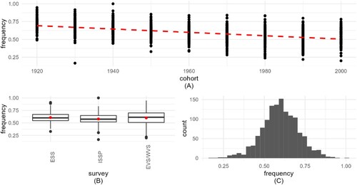
Figure 2. Visualization of implied probability of weekly prayer (IMP_WPR). 2A (top) frequency shows how IMP_WPR decreases by cohort. 2B (bottom left) boxplots present the frequency distribution for the 3 surveys, with medians and means (red circles). 2C (bottom right) histogram shows the distribution of the aggregated variable.

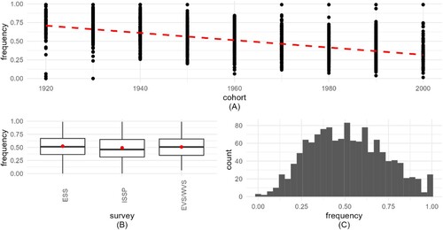
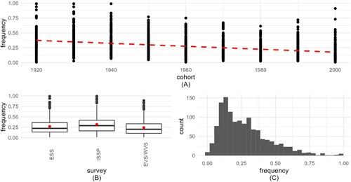
Figure 3. Visualization of implied probability of weekly service attendance (IMP_ATT). 3A (top) frequency shows how IMP_WPR decreases by cohort. 3B (bottom left) boxplots present the frequency distribution for the 3 surveys, with medians and means (red circles). 3C (bottom right) histogram shows the distribution of the aggregated variable.

Figure 2 presents the descriptive information for IMP_WPR (implied probability of weekly prayer).

Figure 3 presents descriptive information for the implied probability of weekly service attendance (IMP_ATT). Figure 3C (bottom right) shows that the variable IMP_ATT is distributed with notable skew.

Descriptive statistics for the three dependent variables show small differences across the surveys, with means close to medians (Table 10). The variable IMP_ATT has the largest differences between means and medians, due to its skew (Figure 3C).

Table 10. Descriptive statistics for IMP_SDR, IMP_WPR, IMP_ATT.

Survey	Mean	Max	Min	Median	Std
IMP_SDR
ESS	0.607	0.909	0.330	0.601	0.0925
ISSP	0.579	1.000	0.167	0.576	0.104
EVS/WVS	0.600	0.948	0.200	0.614	0.142
IMP_WPR
ESS	0.524	0.990	0.000	0.512	0.202
ISSP	0.493	0.990	0.000	0.459	0.235
EVS/WVS	0.508	0.990	0.0625	0.508	0.207
IMP_ATT
ESS	0.270	0.990	0.00962	0.224	0.174
ISSP	0.318	0.990	0.00962	0.289	0.190
EVS/WVS	0.242	0.888	0.0110	0.202	0.170

Analysis 1 – diagnostic model for IMP_SDR, IMP_WPR, and IMP_ATT

To explain variability in the dependent variables, and thereby to evaluate empirical expectations EE1-EE3, we constructed the three models described above. Table 11 presents the analysis of model 1, which is an important test of EE1. The random effects section of Table 11 documents how much variance (τ₀₀) exists between surveys and between countries. In all three cases, the variance attributable to the survey is very small, and dwarfed by the variance attributable to countries. This supports EE1 and suggests that the aggregation method used to create DIM-R is robust, regardless of which survey was used to generate the aggregate values for the three dependent variables.

Table 11. Summary of model 1 for the three aggregate variables (ML estimation method).

	IMP_SDR Model 1		IMP_WPR Model 1		IMP_ATT Model 1
Predictors	Estimates	SE	Estimates	SE	Estimates	SE
(Intercept)	0.6004 ***	0.0147	0.5171 ***	0.0260	0.2820 ***	0.0350
Random Effects
σ^2	0.0078		0.0273		0.0134
τ00 (countries)	0.0049		0.0183		0.0187
τ00 (surveys)	0.0001		0.0000		0.0016
N (countries)	28		28		28
N (surveys)	3		3		3
Observations	1305		1291		1307
Marginal R^2 / Conditional R^2	0.0000 / 0.3922		0.00000 / NA		0.00000 / 0.60261
AIC	−2516.571		−875.515		−1789.567

* p < 0.05 ** p < 0.01 *** p < 0.001.

For model 2, we fitted a linear mixed model (using the mean-likelihood estimation method and nloptwrap optimizer) to predict dependent variables by adding cohort10 (birth cohort) as a fixed effect to model 1. As with model 1, model 2 included country and survey as random effects.

Model 3 is the best relative fit in comparison to models 1 and 2 for dependent variables IMP_SDR and IMP_WPR, based on the lowest AIC value. Model 2 is the best relative fit in comparison to models 1 and 3 for dependent variable IMP_ATT, based on the lowest AIC value. This confirms both EE2 – that adding cohort10 (birth cohort) as a fixed effect would improve model fit – and EE3 – that model 2 can be improved by adding WaveYear as a random effect, keeping country as a random effect, and keeping cohort10 as a fixed effect. Table 12 shows the analysis of models 3 and 2 for all three dependent variables.

Table 12. Summary of best-fit model 3 for variables IMP_SRD and IMP_WPR and model 2 for variable IMP_ATT (ML estimation method).

	IMP_SDR Model 3		IMP_WPR Model 3		IMP_ATT Model 2
Predictors	Estimates	SE	Estimates	SE	Estimates	SE
(Intercept)	5.1852 ***	0.1636	9.9261 ***	0.2863	4.9569 ***	0.2362
cohort10	−0.0023 ***	0.0001	−0.0048 ***	0.0001	−0.0024 ***	0.0001
Random Effects
σ^2	0.00472		0.01448		0.01020
τ00 (countries)	0.00512 cc		0.01886 cc		0.01851 cc
τ00 (WaveYear)	0.00025 WaveYear		0.00030 WaveYear
τ00 (surveys)	0.00010 pm3		0.00001 pm3		0.00160 pm3
N (countries)	28 cc		28 cc		28 cc
N (surveys)	3 pm3		3 pm3		3 pm3
N (WaveYear)	6 WaveYear		6 WaveYear
Observations	1305		1291		1307
Marginal R^2 / Conditional R^2	0.22826 / 0.64224		0.27448 / 0.68779		0.09401 / 0.69507
AIC	−3124.295		−1649.895		−2119.621

* p < 0.05 ** p < 0.01 *** p < 0.001.

In the Appendix, we present a summary of all three models for each dependent variable. Moreover, Tables 11 and 12 were based on the mean-likelihood (ML) estimation method recommended for comparing models among themselves. Marginal R² represents the variance explained by fixed effects, while conditional R² is interpreted as the variance explained by the whole model, including both fixed and random effects. In the Appendix, we also include an evaluation of models using the Restricted Maximum Likelihood Estimation (REML) method. The Appendix’s diagnostic charts show that a skewed dependent variable (such as IMP_ATT) causes the largest deviations from the assumptions.

Analysis 2 – descriptive statistics for IMP_SDR, IMP_WPR, and IMP_ATT

Figures 4, 5, and 6 present descriptive information for the 3 dependent variables IMP_SDR, IMP_WPR, and IMP_ATT, respectively. The interpretation of the graphs is the same as for analysis 1 (Bates et al., 2015).

Figure 4. Visualization of implied self-declared religiosity (IMP_SDR). 4A (top) frequency shows how IMP_SDR decreases by cohort. 4B (bottom left) boxplots present the frequency distribution for the 2 surveys, with medians and means (red circles). 4C (bottom right) histogram shows the distribution of the aggregated variable.

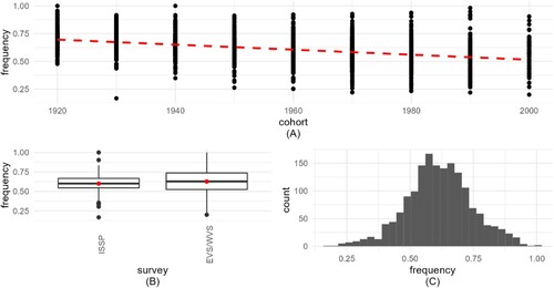
Figure 5. Visualization of implied probability of weekly prayer (IMP_WPR). 5A (top) frequency shows how IMP_WPR decreases by cohort. 5B (bottom left) boxplots present the frequency distribution for the 2 surveys, with medians and means (red circles). 5C (bottom right) histogram shows the distribution of the aggregated variable.

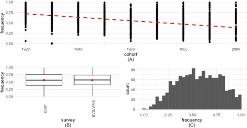
Figure 6. Visualization of implied probability of weekly service attendance (IMP_ATT). 6A (top) frequency shows how IMP_ATT decreases by cohort. 6B (bottom left) boxplots present the frequency distribution for the 2 surveys, with medians and means (red circles). 6C (bottom right) histogram shows the distribution of the aggregated variable.

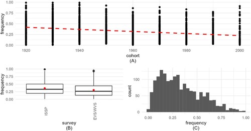
Regardless of the survey, means and medians differ slightly for IMP_SDR and IMP_WPR, and a little more for IMP_ATT (due to skewness). The means differ between the surveys too, for IMP_SDR and especially for IMP_ATT. Additionally, for the IMP_SDR variable in the case of ISSP, we observe slightly less within-survey variance for the countries selected for analysis (Table 13).

Table 13. Descriptive statistics for dependent variables (IMP_SDR, IMP_WPR, IMP_ATT).

Survey	Mean	Max	Min	Median	Std
VARIABLE IMP_SDR
ISSP	0.600	1.000	0.167	0.601	0.0940
EVS/WVS	0.627	1.000	0.200	0.629	0.152
VARIABLE IMP_WPR
ISSP	0.567	0.990	0.000	0.566	0.233
EVS/WVS	0.564	0.990	0.00962	0.570	0.212
VARIABLE IMP_ATT
ISSP	0.365	0.990	0.00962	0.331	0.210
EVS/WVS	0.304	0.949	0.00962	0.265	0.209

Analysis 2 – diagnostic model for IMP_SDR, IMP_WPR, and IMP_ATT

In analysis 2, we built the same three models as in analysis 1 to assess the fit of the data over a longer time frame but excluding ESS. The Appendix presents a summary of models for each of the three dependent variables. Table 14 presents the analysis of model 1, which is an important test of EE1. In all three cases, the variance attributable to the survey is very small, and dwarfed by the variance attributable to countries. As in analysis 1, analysis 2 supports EE1 and suggests that the aggregation method used to create DIM-R is robust, regardless of which survey was used to generate the aggregate values for the three dependent variables.

Table 14. Summary of model 1 for the three dependent variables (ML estimation method).

	IMP_SDR Model 1		IMP_WPR Model 1		IMP_ATT Model 1
Predictors	Estimates	SE	Estimates	SE	Estimates	SE
(Intercept)	0.6228 ***	0.0196	0.5764 ***	0.0279	0.3433 ***	0.0358
Random Effects
σ^2	0.00819		0.02227		0.01420
τ00 (countries)	0.00898		0.02812		0.03180
τ00 (surveys)	0.00027		0.00000		0.00083
N (countries)	37		37		37
N (surveys)	2		2		2
Observations	1668		1423		1681
Marginal R^2 / Conditional R^2	0.00000 / 0.53018		0.00000 / NA		0.00000 / 0.69683
AIC	−3118.449		−1218.937		−2194.617

* p < 0.05 ** p < 0.01 *** p < 0.001.

Model 3 of analysis 2 produced the best relative fit in comparison to models 1 and 2 for each of the three dependent variables (IMP_SDR, IMP_WPR, IMP_ATT) based on the lowest AIC value. This further confirms both EE2 and EE3. Table 15 shows the analysis of model 3 for all three dependent variables. The Appendix presents a comparison of the three models, for each dependent variable.

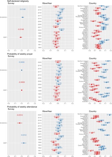
• For the dependent variable IMP_SDR, the random effect of survey explains 2% of the variance, while the random effect of WaveYear explains 6% of the variance and country explains 57% of the variance.

• For the dependent variable IMP_WPR, the random effect of survey explains less than 1% of the variance, while the random effect of WaveYear explains 1% of the variance and country explains 66% of the variance.

• For the dependent variable IMP_ATT, the random effect of survey explains 3% of the variance, while the random effect of WaveYear explains 2% of the variance and country explains 70% of the variance.

  Table 15. Summary of best-fit model 3 for the three dependent variables (ML estimation method).

  	IMP_SDR Model 3		IMP_WPR Model 3		IMP_ATT Model 3
  Predictors	Estimates	SE	Estimates	SE	Estimates	SE
  (Intercept)	5.4180 ***	0.1651	8.7506 ***	0.2825	5.0606 ***	0.2400
  cohort10	−0.0025 ***	0.0001	−0.0042 ***	0.0001	−0.0024 ***	0.0001
  Random Effects
  σ^2	0.00519		0.01374		0.01099
  τ00 (countries)	0.00890 cc		0.02764 cc		0.03158 cc
  τ00 (WaveYear)	0.00104 WaveYear		0.00048 WaveYear		0.00107 WaveYear
  τ00 (surveys)	0.00033 pm3		0.00000 pm3		0.00138 pm3
  N (countries)	37 cc		37 cc		37 cc
  N (surveys)	2 pm3		2 pm3		2 pm3
  N (WaveYear)	15 WaveYear		13 WaveYear		15 WaveYear
  Observations	1668		1423		1681
  Marginal R^2 / Conditional R^2	0.16341 / 0.71904		0.17613 / 0.72958		0.06095 / 0.77070
  AIC	−3807.189		−1855.049		−2567.180

  * p < 0.05 ** p < 0.01 *** p < 0.001.

All models have high explanatory power (72%, 73%, and 77%, respectively) and marginal R2 is 0.16, 0.17, and 0.06, respectively.

Evaluation of empirical expectations

EE1: The three dependent variables (that is, the aggregated variables IMP_SDR, IMP_WPR, and IMP_ATT) do not differ significantly by survey group but do differ significantly by country group, as assessed by a linear mixed model treating as random effects the key categorical variables of country and survey.

This empirical expectation is strongly supported by the two analyses above. The linear mixed models with country and survey as random effects (that is, model 1 in both analyses for all three dependent variables) show that surveys explain very little variance in the dependent variables whereas country explains a large amount of variance.

EE2: The first model (from EE1) is improved by adding a fixed effect of survey participants grouped into ten-year birth cohorts (using the variable cohort10), since we do expect the aggregated variables to depend on birth cohort in a consistent way.

This empirical expectation is strongly supported by both analyses. Adding cohort10 as a fixed effect markedly improved the models in all cases.

EE3: The second model (from EE2) can be improved by adding WaveYear as a random effect, retaining country and survey as random effects, and retaining cohort10 as a fixed effect.

Again, the empirical expectation is strongly supported by the analyses. The model improved the fit by adding WaveYear as a random effect (except for analysis 1, where dependent variable was IMP_ATT and model 2 was a slightly better fit than model 3).

Between-country, between-year, and between-survey effects on dependent variables

The graphs (Figures 7 and 8) allow us to assess how the random effects differ from each other and show their standard errors and present the effect of surveys and countries on the dependent variables (Wickham, 2016). The values of the effects for the survey differ only slightly, while for the countries there are large differences in the random effect values.

Figure 7. Visualization for analysis 1 of the random effect sizes (x-axis) of the three dependent variables explained by the three/two random-effect variables: survey (left column), WaveYear (middle column), and country (right column). The top row shows results for self-declared religiosity, the middle row for the probability of weekly prayer, and the bottom row for the probability of weekly service attendance.

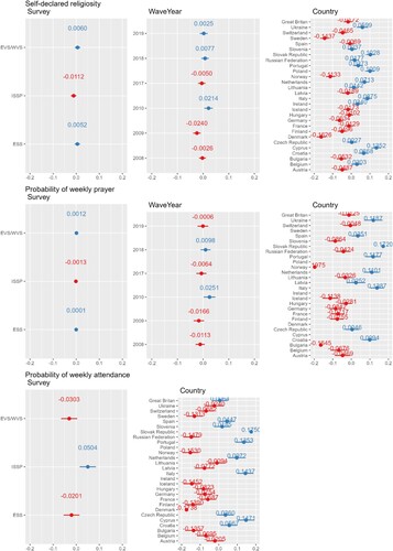
Figure 8. Visualization for analysis 2 of the random effect sizes (x-axis) of the three dependent variables explained by the three random-effect variables: survey (left column), WaveYear (middle column), and country (right column). The top row shows results for self-declared religiosity, the middle row the probability of weekly prayer, and the bottom row for the probability of weekly service attendance.

Discussion

The diagnostic linear mixed models demonstrate the soundness of the method used to harmonize attendance, prayer, and self-described religiosity variables, using the integrated denominational affiliation variable to select countries and Christian respondents. We achieve similar results in descriptive statistics and the variance between surveys and waves is negligible for the three variables (IMP_ATT, IMP_PRAY, IMP_SDR), so we can use the integrated DIM-R dataset with confidence while recognizing its limitations. Despite methodological differences across surveys, and even between countries within a survey, DIM-R’s integrated religious variables are not differentiated at the survey and wave level.

While the focus of this paper is on validating a harmonized dataset covering many periods and places, these preliminary results already demonstrate the usefulness of DIM-R and suggest that the harmonized dataset can be helpful for understanding religious change. This usefulness derives in part from the way DIM-R is structured: it facilitates ready comparison of dimensions of religiosity across age and birth cohorts, countries, and religions. It is also easy to extend. For example, researchers often point to existential security as a cause of declining religiosity (Lüdecke, 2018; Gore et al., 2018). By combining DIM-R with national indicators of existential security over time, it is immediately possible to assess this hypothesis across a great range of societies, as well as drilling down into specific religious groups within those societies. Thus, DIM-R can be used to generate evidence that the underlying process of religious decline is common across countries, notwithstanding differences in their levels of religiosity at any given time. In future work, we plan to use DIM-R to calibrate and validate agent-based computational simulations of the emergence of the macro-level patterns of secularization from the behaviors and interactions of religious, fuzzy, and secular individuals at the micro-level. This will enable us to address major questions in the sociology of religion regarding the causal processes driving secularization and religious change more broadly. A large, varied dataset such as DIM-R is absolutely essential to this kind of work.

Limitations of this study

Although DIM-R opens up many analytical possibilities related to the study of religion, including secularization and religious change, DIM-R also has limitations.

First, DIM-R does not have a full global representation and we did not incorporate local barometers from different regions. DIM-R integrates four large-scale surveys that included sufficient measurement of attendance, prayer, self-described religiosity, and denominational affiliation. Unlike CARPE and SMRE for example, we excluded the Eurobarometer, which includes no data on prayer and only limited data on self-described religiosity. We hope DIM-R will provide a similar foundation for harmonization as CARPE did for us, so that additional repeated cross-sectional datasets can be included and improve global coverage in future harmonization efforts.

An important limitation is the uneven representation of individual countries in DIM-R and the impossibility of conducting reliability analyses on all countries present in DIM-R. Although the full dataset contains 118 countries, it should be noted that 22 were surveyed only once by EVS or WVS or ISSP, while 34 were surveyed at least twice, but only by WVS. In addition, because the ESS is only concerned with European countries, this results in considerably more European than non-European countries in many waves of DIM-R. We cannot guarantee the same level of reliability for the harmonized measures among the subset of countries excluded from the analyses in this paper. Nonetheless, the under-surveyed countries have been included in the full DIM-R dataset because there is considerable utility in preserving all participating countries for future research. Our harmonized measures are applied systematically across participating countries, which enables cross-country comparisons along a common standard and provides a foundation for expanding DIM-R to incorporate additional waves or other cross-sectional surveys. A common standard does not equate to a common meaning: even for Christian-dominated countries, weekly attendance may be relatively normative, but not uniformly expected of the devout. Researchers should acknowledge this fact and interpret results from DIM-R carefully, particularly when comparing results between countries that have been studied only once or twice, or when comparing regions, such as Europe and South America.

In addition, it is necessary to recognize the limitations common to other data harmonization projects (Tomescu-Dubrow & Slomczynski, 2016; Slomczynski & Tomescu-Dubrow, 2018; Norris & Inglehart, 2011; Fortier et al., 2010; Kołczyńska & Slomczynski, 2018; Durand et al., 2017). Some of these common problems are technical, relating to differences in the construction of measurement tools, in the coding of variables, and in the operationalization of indicators. Also, some limitations are methodological, resulting from different data collection procedures using non-identical research techniques, differences in sampling method, sample size, fieldwork, and amount of missing data. Finally, still other limitations are contextual, environmental, or cultural, resulting from differences between countries in characteristics such as the level of literacy (Tomescu-Dubrow & Slomczynski, 2023). These limitations are to be expected as part of the trade-off associated with overriding local peculiarities to increase the temporal and spatial scope of possible analyses.

Researchers must also be aware that the self-declared religiosity variable from the EVS/WVS surveys required additional procedures to harmonize them with ISSP and ESS. We estimated self-declared religiosity based on similar, highly correlated variables, controlled by the available nominal variable defining the respondent's subjective religiosity. Also, the absence of the “pray” question in five of the twelve EVS/WVS waves limits the power of the dataset for this indicator. Moreover, DIM-R includes no harmonization of items related to religious beliefs, which would be useful for understanding the precise nature of religious change, especially in secularizing environments.

Finally, researchers employing DIM-R need to keep in mind that, despite its temporal span, it is not a longitudinal cohort study; it is a harmonization of several cross-sectional surveys. Care must be taken when drawing inferences about religious change, accordingly. For example, DIM-R’s cohort-level indications about the dynamics of religious change are average effects and may mask subtleties within the population. Longitudinal cohort datasets would be needed to produce a fine-grained appreciation for the dynamics of religious change that takes account of the multiple dimensions along which it can occur.

These limitations suggest that, like all datasets, DIM-R cannot be used indiscriminately for analysis, without regard for its distinctive features. We caution potential users to carefully consider the goals of their research projects when evaluating whether DIM-R is an appropriate resource for their analysis.

Conclusions

DIM-R, despite its limitations, is an important new resource for tackling big questions in the scientific study of religion. Its construction reduces the data cleaning burden on future research, and by increasing the number of observations across countries, time, and cohorts, it is possible to track the process of change in particular dimensions of religiosity more comprehensively. In addition, DIM-R provides the opportunity to further explore other constructs, such as indexes based on harmonized variables, by applying novel analysis methods (e.g., machine learning) and incorporating additional variables as needed. Integrating multiple data sources presents unique challenges but offers many rewards. We invite other researchers to extend DIM-R so that future research can make use of the wealth of data that already exist.

Financial disclosure

The research leading to these results has received funding from:

1. The Norway Grants (Award number 2019/34/H/HS1/00654); Grant Recipient: Konrad Talmont-Kaminski.

2. Narodowe Centrum Nauki (Award number UMO-2019/34/H/HS1/00654); Grant Recipient: Konrad Talmont-Kaminski.

3. John Templeton Foundation (Award Number: 61074); Grant Recipient: Wesley J. Wildman.

Disclosure statement

No potential conflict of interest was reported by the author(s).

Additional information

Funding

This work was supported by Narodowe Centrum Nauki: [Grant Number UMO-2019/34/H/HS1/00654]; Norway Grants: [Grant Number 2019/34/H/HS1/00654]; John Templeton Foundation: [Grant Number 61074].

Appendix

Visualizing model 2’s predictions

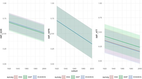
Analysis 1: plotting model 3 predictions for dependent variables (IMP_SDR, IMP_WPR,) and model 2 for dependent variable (IMP_ATT) for all surveys (ESS, ISSP, EVS/WVS)

We will represent model 2 as a regression line with surrounding error. The Figure 9 shows random intercepts and constant slopes for the three surveys and three dependent variables (IMP_SDR, IMP_WPR, and IMP_ATT).

Figure 9. Prediction plots of the three variables for model 3 (IMP_SDR and IMP_WPR) and model 2 (IMP_ATT). This figure illustrates the prediction plots for three key variables obtained from two distinct models. Model 3 focuses on predicting IMP_SDR and IMP_WPR, while Model 2 is dedicated to forecasting IMP_ATT. Each line represents the model's prediction over a specified time period, and the corresponding shaded regions indicate the associated confidence intervals. The x-axis denotes the cohorts, while the y-axis represents the predicted values. The comparison between the predicted values and actual observations offers insights into the model's accuracy and reliability in forecasting both IMP_SDR, IMP_WPR, and IMP_ATT.

Analysis 2: plotting model 2 predictions for dependent variables (IMP_SDR, IMP_WPR, IMP_ATT) for all surveys (ESS, ISSP, EVS/WVS)

REML estimates for model 3 (IMP_SDR, IMP_WPR) and model 2 (IMP_ATT)

Analysis 1: REML estimation for diagnostic model for three dependent variables (IMP_SDR, IMP_WPR, IMP_ATT)

Table 16 summarizes the 3 dependent variables with REML estimation for the third and second models.

Table 16. Summary of 3 dependent variables with REML estimation for model three and two.

	IMP_SDR Model 3		IMP_WPR Model 3		IMP_ATT Model 2
Predictors	Estimates	SE	Estimates	SE	Estimates	SE
(Intercept)	5.1855 ***	0.1637	9.9261 ***	0.2863	4.9568 ***	0.2366
cohort10	−0.0023 ***	0.0001	−0.0048 ***	0.0001	−0.0024 ***	0.0001
Random Effects
σ^2	0.00473		0.01448		0.01021
τ00 (country)	0.00526 cc		0.01886 cc		0.01890 cc
τ00 (WaveYEar)	0.00026 WaveYear		0.00030 WaveYear
τ00 (survey)	0.00011 pm3		0.00001 pm3		0.00197 pm3
N (country)	28 cc		28 cc		28 cc
N (survey)	3 pm3		3 pm3		3 pm3
N (WaveYear)	6 WaveYear		6 WaveYear
Observations	1305		1291		1307
Marginal R^2 / Conditional R^2	0.22551 / 0.64633		0.27448 / 0.68779		0.09191 / 0.70163
AIC	−3124.311		−1649.895		−2119.670

* p < 0.05 ** p < 0.01 *** p < 0.001.

Table 17 shows the variance partition coefficient for the three variables IMP_SDR, IMP_WPR, and IMP_ATT (Figures 10, 11, 12, 13, 14, 15, and 16).

Figure 10. Prediction plots of the three variables for model 3. This figure illustrates the prediction plots for three key variables obtained from two distinct models. Model 3 focuses on predicting IMP_SDR, IMP_WPR, and IMP_ATT. Each line represents the model's prediction over a specified time period, and the corresponding shaded regions indicate the associated confidence intervals. The x-axis denotes the cohorts, while the y-axis represents the predicted values. The comparison between the predicted values and actual observations offers insights into the model's accuracy and reliability in forecasting both IMP_SDR, IMP_WPR, and IMP_ATT.

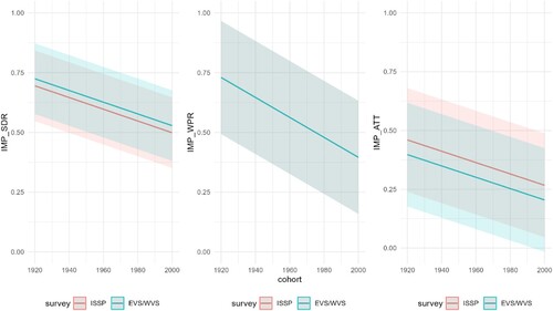
Figure 11. Diagnostic charts for the third model with the dependent variable IMP_SDR. The PPC chart can show the actual observations compared to the data generated by the model. This allows you to assess whether the distributions of the generated data are consistent with the actual data. The Linearity chart shows whether the residuals are evenly distributed along the x-axis. If the residuals are random and show no pattern to the predicted values, this suggests that the model captures the linearity of the relationship between the variables well. The Homogeneity of Variance chart helps assess whether the variances of the residuals are equal for different levels of predicted values. The Normality of Residuals chart shows whether the residuals of the model have a normal distribution. The trend line should be close to a straight line. Separate Random Effects Normality charts for the country, survey and WaveYear categories allow you to assess whether the random effects for different levels of these variables have a normal distribution. The Influential Observations chart identifies observations that can significantly affect model parameter estimates.

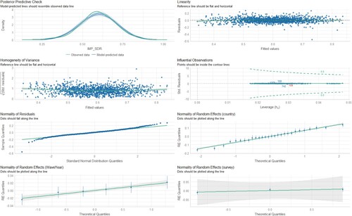
Figure 12. Diagnostic charts for the third model with the dependent variable IMP_WPR. The PPC chart can show the actual observations compared to the data generated by the model. This allows you to assess whether the distributions of the generated data are consistent with the actual data. The Linearity chart shows whether the residuals are evenly distributed along the x-axis. If the residuals are random and show no pattern to the predicted values, this suggests that the model captures the linearity of the relationship between the variables well. The Homogeneity of Variance chart helps assess whether the variances of the residuals are equal for different levels of predicted values. The Normality of Residuals chart shows whether the residuals of the model have a normal distribution. The trend line should be close to a straight line. Separate Random Effects Normality charts for the country, survey and WaveYear categories allow you to assess whether the random effects for different levels of these variables have a normal distribution. The Influential Observations chart identifies observations that can significantly affect model parameter estimates.

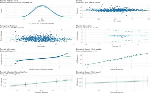
Figure 13. Diagnostic charts for the second model with the dependent variable IMP_ATT. The PPC chart can show the actual observations compared to the data generated by the model. This allows you to assess whether the distributions of the generated data are consistent with the actual data. The Linearity chart shows whether the residuals are evenly distributed along the x-axis. If the residuals are random and show no pattern to the predicted values, this suggests that the model captures the linearity of the relationship between the variables well. The Homogeneity of Variance chart helps assess whether the variances of the residuals are equal for different levels of predicted values. The Normality of Residuals chart shows whether the residuals of the model have a normal distribution. The trend line should be close to a straight line. Separate Random Effects Normality charts for the country, survey and WaveYear categories allow you to assess whether the random effects for different levels of these variables have a normal distribution. The Influential Observations chart identifies observations that can significantly affect model parameter estimates.

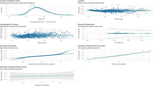
Figure 14. Diagnostic charts for the third model with the dependent variable IMP_SDR. The PPC chart can show the actual observations compared to the data generated by the model. This allows you to assess whether the distributions of the generated data are consistent with the actual data. The Linearity chart shows whether the residuals are evenly distributed along the x-axis. If the residuals are random and show no pattern to the predicted values, this suggests that the model captures the linearity of the relationship between the variables well. The Homogeneity of Variance chart helps assess whether the variances of the residuals are equal for different levels of predicted values. The Normality of Residuals chart shows whether the residuals of the model have a normal distribution. The trend line should be close to a straight line. Separate Random Effects Normality charts for the country, survey and WaveYear categories allow you to assess whether the random effects for different levels of these variables have a normal distribution. The Influential Observations chart identifies observations that can significantly affect model parameter estimates.

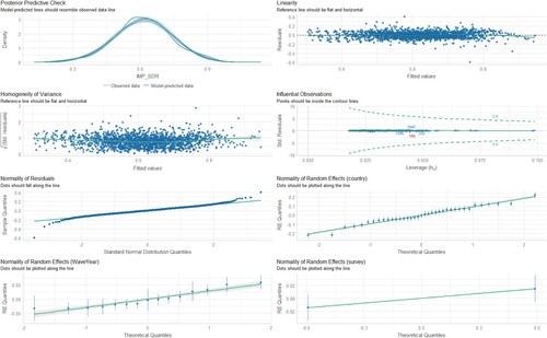
Figure 15. Diagnostic charts for the third model with the dependent variable IMP_WPR. The PPC chart can show the actual observations compared to the data generated by the model. This allows you to assess whether the distributions of the generated data are consistent with the actual data. The Linearity chart shows whether the residuals are evenly distributed along the x-axis. If the residuals are random and show no pattern to the predicted values, this suggests that the model captures the linearity of the relationship between the variables well. The Homogeneity of Variance chart helps assess whether the variances of the residuals are equal for different levels of predicted values. The Normality of Residuals chart shows whether the residuals of the model have a normal distribution. The trend line should be close to a straight line. Separate Random Effects Normality charts for the country, survey and WaveYear categories allow you to assess whether the random effects for different levels of these variables have a normal distribution. The Influential Observations chart identifies observations that can significantly affect model parameter estimates.

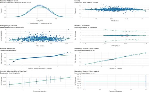
Figure 16. Diagnostic charts for the third model with the dependent variable IMP. The PPC chart can show the actual observations compared to the data generated by the model. This allows you to assess whether the distributions of the generated data are consistent with the actual data. The Linearity chart shows whether the residuals are evenly distributed along the x-axis. If the residuals are random and show no pattern to the predicted values, this suggests that the model captures the linearity of the relationship between the variables well. The Homogeneity of Variance chart helps assess whether the variances of the residuals are equal for different levels of predicted values. The Normality of Residuals chart shows whether the residuals of the model have a normal distribution. The trend line should be close to a straight line. Separate Random Effects Normality charts for the country, survey and WaveYear categories allow you to assess whether the random effects for different levels of these variables have a normal distribution. The Influential Observations chart identifies observations that can significantly affect model parameter estimates.

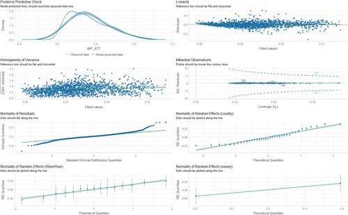
Table 17. Variance partition coefficient.

	VPC FOR REML MODELS ESTIMATION
	IMP_SDR	IMP_WPR	IMP_ATT
CC	0.508	0.560	0.608
WAVEYEAR	0.024	0.009	–
PM3	0.010	0.0002	0.063
RESIDUAL	0.457	0.445	0.329

Analysis 2: REML estimation for diagnostic model for three dependent variables (IMP_SDR, IMP_WPR, IMP_ATT)

Table 18 summarizes the 3 dependent variables with REML estimation for the third model.

Table 18. Summary of 3 dependent variables with REML estimation for model three.

	IMP_SDR Model 3		IMP_WPR Model 3		IMP_ATT Model 3
Predictors	Estimates	SE	Estimates	SE	Estimates	SE
(Intercept)	5.4183 ***	0.1654	8.7514 ***	0.2826	5.0608 ***	0.2407
cohort10	−0.0025 ***	0.0001	−0.0042 ***	0.0001	−0.0024 ***	0.0001
Random Effects
σ^2	0.00519		0.01375		0.01100
τ00 (country)	0.00902 cc		0.02837 cc		0.03204 cc
τ00 (WaveYear)	0.00105 WaveYear		0.00049 WaveYear		0.00108 WaveYear
τ00 (survey)	0.00045 pm3		0.00000 pm3		0.00199 pm3
N (country)	37 cc		37 cc		37 cc
N (survey)	2 pm3		2 pm3		2 pm3
N (WaveYear)	15 WaveYear		13 WaveYear		15 WaveYear
Observations	1668		1423		1681
Marginal R^2 / Conditional R^2	0.16112 / 0.72285		0.17360 / 0.73333		0.05961 / 0.77564
AIC	−3807.243		−1855.060		−2567.256

* p < 0.05 ** p < 0.01 *** p < 0.001.

Table 19 shows the variance partition coefficient for the three variables IMP_SDR, IMP_WPR, and IMP_ATT.

Table 19. Variance partition coefficient.

	VPC FOR REML MODELS ESTIMATION
	IMP_SDR	IMP_WPR	IMP_ATT
CC	0.574	0.666	0.695
WAVEYEAR	0.066	0.011	0.023
PM3	0.028	0.0000000740	0.043
RESIDUAL	0.330	0.323	0.239

Results for linear mixed models for the three dependent variables

Analysis 1: DIM-R results for IMP_SDR

For the IMP_SDR variable, we created 3 models and then compared them.

Model 1: Random effect only with variables: country and survey.

Model 2: Add fixed effect with variable cohort.

Model 3: Add random effects model with variables: country and survey and WaveYear, and add fixed effect with variable cohort.

The mixed model allows us to take into account the observed structure of the data. It allows us to better understand the sources of variation in the dependent variable. We also obtain model parameter estimates for individual groups; in our case these are surveys, countries, and WaveYear, which allows us to understand exactly how these groups differ from each other. This, in turn, allows for group-specific predictions and thus a much more accurate prediction, assuming there is substantial variance due to clustering. Table 20 presents three alternative approaches to multilevel estimation.

Table 20. Summary of the three models for the dependent variable IMP_SDR.

	Model 1		Model 2		Model 3
Predictors	Estimates	SE	Estimates	SE	Estimates	SE
(Intercept)	0.6004 ***	0.0147	5.1010 ***	0.1621	5.1852 ***	0.1636
cohort10			−0.0023 ***	0.0001	−0.0023 ***	0.0001
Random Effects
σ^2	0.00780		0.00485		0.00472
τ00 (country)	0.00493 cc		0.00478 cc		0.00512 cc
τ00 (survey)	0.00010 pm3		0.00011 pm3		0.00010 pm3
τ00 (WaveYear)					0.00025 WaveYear
N (country)	28 cc		28 cc		28 cc
N (survey)	3 pm3		3 pm3		3 pm3
N (WaveYear)					6 WaveYear
Observations	1305		1305		1305
Marginal R^2 / Conditional R^2	0.00000 / 0.39216		0.22985 / 0.61630		0.22826 / 0.64224
AIC	−2516.571		−3104.628		−3124.295

* p < 0.05 ** p < 0.01 *** p < 0.001.

Table 20 summarizes the 3 models for the dependent variable IMP_SDR.

When comparing the AIC for each of the models presented, model 3 was found to be the best fit and the results are described on it. For the model the fixed effect score of the mean is 5.4180. In addition, the models were compared to each other using the ranova() test, where significant differences were observed, with the third model being the best fit (p < 0.001). We see that the random effect for countries is significant (p < 0.001), the random effect for WaveYear is significant (p < 0.001) and the random effect for surveys is significant (p < 0.001).

The random effects variance, σ², represents the average variance of the random effects of the model. This variance reflects the “average” variance of the random effects for mixed models. For simple random coefficient models, the random effects variance is equal to the variance of the random coefficient. The random-effects variance estimate is 0.00472. The fixed effect of cohorts is −0.0023, the amount by which religiosity is lower on average when moving from cohort to cohort.

The random effect section contains the results of estimating the parameters of the random effect variance. Estimates of the variance of countries, surveys, and WaveYear are given in turn. The results tell how large the variance is between the levels of the clustering factors (between countries between surveys and between WaveYear), plus the residual variance.

VPC_cc – the quotient of variance for countries is 0.00512 /(0.00472 + 0.00512 + 0.00010 + 0.00025) = 0.50245.

VPC_pm3 – the quotient of variance for the surveys is 0.00010 /(0.00472 + 0.00512 + 0.00010 + 0.00025) = 0.00981. As shown in VPC_pm3, the proportion of variance due to differences between surveys is less than 1%.

VPC_WaveYear – the quotient of variance for the surveys is 0.00025/(0.00472 + 0.00512 + 0.00010 + 0.00025) = 0.02453. As shown in VPC_pm3, the proportion of variance due to differences between surveys is only 2%.

This confirms the slight effect of surveys and WaveYear on the results for IMP_SDR in the harmonized base.

Analysis 1: DIM-R results for IMP_WPR

As for IMP_SDR, we also build three diagnostic models for IMP_WPR. The Table 21 shows three alternative approaches to multilevel estimation: Model 1: Random effect only with variables country and survey; Model 2: Add fixed effect with variable cohort; Model 3: Random effects model with country, survey, and WaveYear and fixed effect for cohort.

Table 21. Summary of the three models for the dependent variable IMP_WPR.

	Model 1		Model 2		Model 3
Predictors	Estimates	SE	Estimates	SE	Estimates	SE
(Intercept)	0.5171 ***	0.0260	9.8219 ***	0.2827	9.9261 ***	0.2863
cohort10			−0.0047 ***	0.0001	−0.0048 ***	0.0001
Random Effects
σ^2	0.02730		0.01464		0.01448
τ00 (country)	0.01831 cc		0.01762 cc		0.01886 cc
τ00 (survey)	0.00000 pm3		0.00001 pm3		0.00001 pm3
τ00 (WaveYear)					0.00030 WaveYear
N (country)	28 cc		28 cc		28 cc
N (survey)	3 pm3		3 pm3		3 pm3
N (WaveYear)					6 WaveYear
Observations	1291		1291		1291
Marginal R^2 / Conditional R^2	0.00000 / NA		0.27854 / 0.67270		0.27448 / 0.68779
AIC	−875.515		−1645.081		−1649.895

* p < 0.05 ** p < 0.01 *** p < 0.001.

Table 21 summarizes the 3 models for the dependent variable IMP_WPR.

The lowest AIC value is observed for the third model, based on which the results will be described. In model 3 the fixed effect score of the mean is 9.9261. The random intercept variance (τ₀₀) for country = 0.01886, for survey = 0.00001, and for WaveYear = 0.00030. The fixed effect of cohorts is −0.0048, which means that on average this is how much lower the IMP_WPR variable is in the next cohort. Here we observe twice the decrease compared to the IMP_SDR variable.

VPC_country – the quotient of variance for countries is 0.01886 /(0.01448 + 0.01886 + 0.00001 + 0.00030) = 0.56048.

VPC_survey – the quotient of variance for surveys is 0.00001 /(0.01448 + 0.01886 + 0.00001 + 0.00030) = 0.0003.

VPC_waveYear – the quotient of variance for surveys is 0.00030 /(0.01448 + 0.01886 + 0.00001 + 0.00030) = 0.00892.

As shown in VPC_survey, the proportion of variance due to differences between surveys is only 0.03% and differences between WaveYear is only 0.8%. This confirms the slight effect of surveys and WaveYear on the results in the harmonized base. Differences between countries explain 56% of the variance remaining after the variance explained by fixed effects (cohort effect).

Analysis 1: DIM-R results for IMP_ATT

Table 22 summarizes the 3 models for the dependent variable IMP_ATT.

Table 22. Summary of the three models for the dependent variable IMP_ATT.

	Model 1		Model 2		Model 3
Predictors	Estimates	SE	Estimates	SE	Estimates	SE
(Intercept)	0.2820 ***	0.0350	4.9569 ***	0.2362	4.9670 ***	0.2388
cohort10			−0.0024 ***	0.0001	−0.0024 ***	0.0001
Random Effects
σ^2	0.01340		0.01020		0.01017
τ00 (country)	0.01868 cc		0.01851 cc		0.01871 cc
τ00 (survey)	0.00163 pm3		0.00160 pm3		0.00165 pm3
τ00 (WaveYear)					0.00005 WaveYear
N (country)	28 cc		28 cc		28 cc
N (survey)	3 pm3		3 pm3		3 pm3
N (WaveYear)					6 WaveYear
Observations	1307		1307		1307
Marginal R^2 / Conditional R^2	0.00000 / 0.60261		0.09401 / 0.69507		0.09364 / 0.69855
AIC	−1789.567		−2119.621		−2118.590

* p < 0.05 ** p < 0.01 *** p < 0.001.

Model 2 for the variable IMP_ATT is the best fit. The fixed effect score of the mean is 4.9569. Random intercept variance (τ₀₀) for country = 0.01851 and for survey = 0.00160. The fixed effects variance, σ² for this model equals 0.003145884. The evaluation of the variance of the random disturbance is 0.02011325. The fixed effect of the cohorts reached −0.0024.

VPC_cc – the quotient of variance for countries is 0.01851/(0.010204 + 0.01851 + 0.00160) = 0.61060896.

VPC_pm3 – the quotient of variance for surveys is 0.00160/(0.010204 + 0.01851 + 0.00160) = 0.052780893. As shown in VPC_pm3, the proportion of variance due to differences between surveys is 5%. This confirms the insignificant effect of surveys on the results in the harmonized base. Differences between countries explain with this variable 61% of the variance remaining after the variance explained by fixed effects (cohort effect).

Analysis 2: DIM-R results for IMP_SDR

Table 23 summarizes the 3 models for the dependent variable IMP_SDR in the second analysis.

Table 23. Summary of the three models for the dependent variable IMP_SDR

	Model 1		Model 2		Model 3
Predictors	Estimates	SE	Estimates	SE	Estimates	SE
(Intercept)	0.6228 ***	0.0196	4.9797 ***	0.1631	5.4180 ***	0.1651
cohort10			−0.0022 ***	0.0001	−0.0025 ***	0.0001
Random Effects
σ^2	0.00819		0.00567		0.00519
τ00 (country)	0.00898 cc		0.00901 cc		0.00890 cc
τ00 (survey)	0.00027 pm3		0.00027 pm3		0.00033 pm30
τ00 (WaveYear)					.00104 WaveYear
N (country)	37 cc		37 cc		37 cc
N (survey)	2 pm3		2 pm3		2 pm3
N (WaveYear)					15 WaveYear
Observations	1668		1668		1668
Marginal R^2 / Conditional R^2	0.00000 / 0.53018		0.14277 / 0.67473		0.16341 / 0.71904
AIC	−3118.449		−3698.618		−3807.189

* p < 0.05 ** p < 0.01 *** p < 0.001.

Analysis 2: DIM-R results for IMP_WPR

Table 24 summarizes the 3 models for the dependent variable IMP_WPR in the second analysis.

Table 24. Summary of the three models for the dependent variable IMP_WPR.

	Model 1		Model 2		Model 3
Predictors	Estimates	SE	Estimates	SE	Estimates	SE
(Intercept)	0.5764 ***	0.0279	8.3621 ***	0.2754	8.7506 ***	0.2825
cohort10			−0.0040 ***	0.0001	−0.0042 ***	0.0001
Random Effects
σ^2	0.02227		0.01408		0.01374
τ00 (country)	0.02812 cc		0.02748 cc		0.02764 cc
τ00 (survey)	0.00000 pm3		0.00004 pm3		0.00000 pm3
τ00 (WaveYear)					0.00048 WaveYear
N (country)	37 cc		37 cc		37 cc
N (survey)	2 pm3		2 pm3		2 pm3
N (WaveYear)					13 WaveYear
Observations	1423		1423		1423
Marginal R^2 / Conditional R^2	0.00000 / NA		0.16324 / 0.71683		0.17613 / 0.72958
AIC	−1218.937		−1836.668		−1855.049

* p < 0.05 ** p < 0.01 *** p < 0.001.

Analysis 2: DIM-R results for IMP_ATT

Table 25 summarizes the 3 models for the dependent variable IMP_ATT in the second analysis.

Table 25. Summary of the three models for the dependent variable IMP_ATT.

	Model 1		Model 2		Model 3
Predictors	Estimates	SE	Estimates	SE	Estimates	SE
(Intercept)	0.3433 ***	0.0358	4.6341 ***	0.2348	4.6077 ***	0.2407
cohort10			−0.0022 ***	0.0001	−0.0022 ***	0.0001
Random Effects
σ^2	0.01420		0.01175		0.01213
τ00(country)	0.03180 cc		0.03129 cc		0.06571 0.01944
τ00(survey)	0.00083 pm3		0.00086 pm3
τ11(country cohort interaction)					0.00000 cc.cohort10
ρ01					−1.00000 cc.1
N (country)	37 cc		37 cc		37 cc
N (survey)	2 pm3		2 pm3
Observations	1681		1681		1681
Marginal R^2 / Conditional R^2	0.00000 / 0.69683		0.05219 / 0.74620		0.16468 / NA
AIC	−2194.617		−2487.026		−2407.967

* p < 0.05 ** p < 0.01 *** p < 0.001.

Diagnostic charts for model 2

The diagnostic figures of model two are included below:

Analysis 1: Diagnostic charts for the third model with the dependent variable IMP_SDR.

Analysis 1: Diagnostic charts for the third model with the dependent variable IMP_WPR.

Analysis 1: Diagnostic charts for the second model with the dependent variable IMP_ATT.

Analysis 2: Diagnostic charts for the second model with the dependent variable IMP_SDR.

Analysis 2: Diagnostic charts for the second model with the dependent variable IMP_WPR.

Analysis 2: Diagnostic charts for the second model with the dependent variable IMP_ATT.

References

- Aizpurua, E., Fitzgerald, R., de Barros, J. F., Giacomin, G., Lomazzi, V., Luijkx, R., Maineri, A., & Negoita, D. (2022). Exploring the feasibility of ex-post harmonisation of religiosity items from the European social survey and the European values study. Measurement Instruments for the Social Sciences, 4(1), 1–23. https://doi.org/10.1186/s42409-022-00038-x
- Bates, D., Mächler, M., Bolker, B., & Walker, S. (2015). Fitting linear mixed-effects models usinglme4. Journal of Statistical Software, 67(1), 1–48. https://doi.org/10.18637/jss.v067.i01
- Biolcati, F., Molteni, F., Quandt, M., & Vezzoni, C. (2022). Church attendance and religious change pooled European dataset (CARPE): A survey harmonization project for the comparative analysis of long-term trends in individual religiosity. Quality & Quantity, 56, 1729–1753. https://doi.org/10.1007/s11135-020-01048-9
- Bruce, S. (2013). Secularization. In Defence of an unfashionable theory (Reprint edition) (256 p.). Oxford University Press.
- Burkhauser, R. V., & Lillard, D. R. (2005). The contribution and potential of data harmonization for cross-national comparative research. Journal of Comparative Policy Analysis: Research and Practice, 7(4), 313–330. https://doi.org/10.1080/13876980500319436
- Durand, C., Peña Ibarra, L. P., Rezgui, N., & Wutchiett, D. (2021). How to combine and analyze all the data from diverse sources: A multilevel analysis of institutional trust in the world. Quality & Quantity, 56, 1755–1797. https://doi.org/10.1007/s11135-020-01088-1
- Durand, C., Valois, I., & Pena Ibarra, L. (2017). Harmonize or control? The Use of multilevel analysis to analyze trust in institutions in the world. Harmon Newsl Surv Data Hamonization Soc Sci, (2), 4–11.
- Fortier, I., Burton, P. R., Robson, P. J., Ferretti, V., Little, J., L’Heureux, F., Deschenes, M., Knoppers, B. M., Doiron, D., Keers, J. C., Linksted, P., Harris, J. R., Lachance, G., Boileau, C., Pedersen, N. L., Hamilton, C. M., Hveem, K., Borugian, M. J., Gallagher, R. P., … Hudson, T. J. (2010). Quality, quantity and harmony: The DataSHaPER approach to integrating data across bioclinical studies. International Journal of Epidemiology, 39(5), 1383–1393. https://doi.org/10.1093/ije/dyq139
- Fortier, I., Doiron, D., Little, J., Ferretti, V., L’Heureux, F., Stolk, R. P., Knoppers, B. M., Hudson, T. J., & Burton, P. R. (2011). Is rigorous retrospective harmonization possible? Application of the DataSHaPER approach across 53 large studies. International Journal of Epidemiology, 40(5), 1314–1328. https://doi.org/10.1093/ije/dyr106
- GESIS. (2023). Leibniz Institute for the Social Sciences. [cited 7 Jul 2023]. Available: https://www.gesis.org/en/services/processing-and-analyzing-data/data-harmonisation/onbound.
- Gore, R., Lemos, C., Shults, F. L., & Wildman, W. J. (2018). Forecasting changes in religiosity and existential security with an agent-based model. Journal of Artificial Societies and Social Simulation, 21(1), 1–31. https://doi.org/10.18564/jasss.3596
- Granda, P., & Blasczyk, E. (2010). XIII. Data Harmonisation. undefined. [cited 7 Apr 2022]. Available: https://www.semanticscholar.org/paper/XIII.-Data-Harmonisation-Granda-Blasczyk/917cede744a7381de7fb692690d83affcc64e707.
- Granda, P., Wolf, C., & Hadorn, R. (2010). Harmonizing survey data. In J. A. Harkness, M. Braun, B. Edwards, T. P. Johnson, L. Lyberg, & P. Mohler (Eds.), Survey methods in multinational, multiregional, and multiculturalcontexts (pp. 315–332). John Wiley & Sons, Inc. https://doi.org/10.1002/9780470609927.ch17
- Greeley, A. M. (1972). Unsecular Man: The persistence of religion (1st ed.). Schocken Books.
- Hackett, C. (2014). Seven things to consider when measuring religious identity. Religion, 44(3), 396–413. https://doi.org/10.1080/0048721X.2014.903647
- Heelas, P., Woodhead, L., Seel, B., Szerszynski, B., & Tusting, K. (2005). The spirituality revolution – why religion is giving way to spirituality. Blackwell. Spiritual Health Int. 2005;6: 191–192. https://doi.org/10.1002/shi.13.
- Hout, M., & Greeley, A. M. (1987). The center doesn’t hold: Church attendance in the United States, 1940–1984. American Sociological Review, 52(3), 325–345. https://doi.org/10.2307/2095353
- Kołczyńska, M., & Slomczynski, K. M. (2018). Item metadata as controls for Ex post harmonisation of international survey projects. In T. P. Johnson, B.-E. Pennell, I. A. L. Stoop, & B. Dorer (Eds.), Advances in comparative survey methods (pp. 1011–1033). John Wiley & Sons, Inc. https://doi.org/10.1002/9781118884997.ch46
- Luckmann, T. (1968). The Invisible Religion: The Problem of Religion in Modern Society. https://doi.org/10.2307/2092407
- Luzern, U. (2023). Swiss Metadatabase of Religious Affiliation in Europe (SMRE). In: Universität Luzern [Internet]. [cited 7 Jul 2023]. Available: https://www.unilu.ch/fakultaeten/ksf/institute/zentrum-fuer-religion-wirtschaft-und-politik/forschung/swiss-metadatabase-of-religious-affiliation-in-europe-smre/.
- Lüdecke, D. (2018). Ggeffects: Tidy data frames of marginal effects from regression models. Journal of Open Source Software, 3(26), 1–5. https://doi.org/10.21105/joss.00772
- May, A., Werhan, K., Bechert, I., Quandt, M., Schnabel, A., & Behrens, K. (2021). ONBound-Harmonisation User Guide (Stata/SPSS), Version 1.1. GESIS Pap. https://doi.org/10.21241/SSOAR.72442
- Norris, P., & Inglehart, R. (2011). Sacred and secular: Religion and politics worldwide (2nd ed). Cambridge University Press. https://doi.org/10.1017/CBO9780511894862
- Oleksiyenko, O., Wysmulek, I., & Vangeli, A. (2018). Identification of processing errors in cross-national surveys. In T. P. Johnson, B.-E. Pennell, I. A. L. Stoop, & B. Dorer (Eds.), Advances in comparative survey methods (pp. 985–1010). John Wiley & Sons, Inc. https://doi.org/10.1002/9781118884997.ch45
- Pollack, D., & Rosta, G. (2017). Religion and modernity: An international comparison. Oxford University Press. https://doi.org/10.1093/oso/9780198801665.001.0001
- Puga-Gonzalez, I., Voas, D., Kiszkiel, L., Bacon, R. J., Wildman, W. J., Talmont-Kaminski, K., & Shults, F. L. (2022). Modeling fuzzy fidelity: Using microsimulation to explore Age, period, and cohort effects in secularization. Journal of Religion and Demography, 9(1-2), 111–137. https://doi.org/10.1163/2589742x-bja10012
- Slomczynski, K. M., & Tomescu-Dubrow, I. (2018). Basic principles of survey data recycling. In T. P. Johnson, B.-E. Pennell, I. A. L. Stoop, & B. Dorer (Eds.), Advances in comparative survey methods (pp. 937–962). John Wiley & Sons, Inc. https://doi.org/10.1002/9781118884997.ch43
- Stark, R., & Iannaccone, L. R. (1994). A supply-side reinterpretation of the “secularization” of Europe. Journal for the Scientific Study of Religion, 33(3), 230–252. https://doi.org/10.2307/1386688
- Stolz, J. (2020). Secularization theories in the twenty-first century: Ideas, evidence, and problems. Presidential address. Social Compass, 67(2), 282–308. https://doi.org/10.1177/0037768620917320
- Tomescu-Dubrow, I., & Slomczynski, K. M. (2016). Harmonization of cross-national survey projects on political behavior: Developing the analytic framework of survey data recycling. International Journal of Sociology, 46(1), 58–72. https://doi.org/10.1080/00207659.2016.1130424
- Tomescu-Dubrow, I., & Slomczynski, K. M. (2023). Democratic values and protest behavior: Data harmonisation, measurement comparability, and multi-level modeling in cross-national perspective. 2014 [cited 7 Jul 2023]. Available: https://kb.osu.edu/handle/1811/69606.
- Voas, D. (2007). Surveys of behaviour, beliefs and affiliation: Micro-quantitative. The SAGE handbook of the sociology of religion (pp. 144–166). SAGE Publications Ltd. https://doi.org/10.4135/9781848607965.n8
- Voas, D. (2008). The rise and fall of fuzzy fidelity in Europe. European Sociological Review, 25(2), 155–168. https://doi.org/10.1093/esr/jcn044
- Voas, D., & Chaves, M. (2016). Is the United States a counterexample to the secularization thesis? American Journal of Sociology, 121(5), 1517–1556. https://doi.org/10.1086/684202
- Wickham, H. (2016). Ggplot2: Elegant graphics for data analysis (2nd ed. 2016 edition). Springer.
- Wolf, C., Schneider, S. L., Behr, D., & Joye, D. (2016). Harmonizing survey questions between cultures and over time. The SAGE handbook of survey methodology. (pp. 502–524). SAGE Publications Ltd. https://doi.org/10.4135/9781473957893.n33
- Wysmułek, I. (2019). Using public opinion surveys to evaluate corruption in Europe: Trends in the corruption items of 21 international survey projects, 1989–2017. Quality & Quantity, 53(5), 2589–2610. https://doi.org/10.1007/s11135-019-00873-x
- Wysmułek, I., Tomescu-Dubrow, I., & Kwak, J. (2022). Ex-post harmonization of cross-national survey data: Advances in methodological and substantive inquiries. Quality & Quantity, 56, 1701–1708. https://doi.org/10.1007/s11135-021-01187-7