Deep automatic soil roughness estimation from digital images

ABSTRACT

Soil roughness, defined as the irregularities of the soil surface, yields significant information about soil water storage, infiltration and overland flow and, thus, is a key factor in characterizing the quality of the terrain; it is often used as input in many synthetic general agricultural models and in particular in soil moisture estimation models. In this paper, we propose a framework that combines a specific setup for data acquisition with deep convolutional networks for actual estimation. The former relies on projecting a line red laser beam on the analysed soil surface followed by digital color image acquisition. The later, involves two convolutional models that are trained in a supervised manner to predict the soil roughness. The data set was produced in the laboratory both on synthetic and real soil samples. The labels used in the training process are the soil roughness values measured by using a pinboard. The detailed evaluation showed that the error of the automatic precision lies in the range of ground truth deviation, thus validating the proposed procedure.

KEYWORDS:

• Soil roughness
• convolutional neural networks
• VGG-11
• ResNet-18

Introduction

The Remote Sensing (RS) domain opened incredible possibilities for the analysis and monitoring of the land cover of our planet. RS data from in-site, proximal or satellite-level measurements offer precious information regarding the soil conditions, vegetation status or health of the agricultural crops. Agriculture 5.0 or shortly, AG5.0, fosters the latest cutting-edge technologies from various domains (Connolly, 2022), including the ones from the domain of Artificial Intelligence (AI) for smart decision-making processes: i) automatic estimation of site-specific soil or crop requirements in terms of water and nutrients, ii) elaboration of farming strategies regarding the control of chemical and mechanical treatments, iii) yield and price estimation by deploying AI-based intelligent decision support systems and, last, but not least, future deployment of agri-robots to replace farmers for various tasks (e.g. sowing or harvesting) (Latief & Firasath, 2021). AI-based transformation in agriculture aims at improving the traditional farming practices by automation and usage of nowadays technologies in order to reduce the intrinsic risks, enable sustainability and predictability for the final goal of enabling a more productive agriculture (Latief & Firasath, 2021).

In the AG5.0 context, the acquisition of information about the agricultural crops is performed at three levels: ground, aerial and satellite, for specific tasks of precision agriculture. Ground measurements, like chlorophyll level (Shapiro et al., 2013), sugar content of tubers and related parameters (NO₃ – glucose, K, Ca₂, Na+, pH), anthocyanin (Morris & Wang, 2007), CO₂ and H₂O flux in photosynthesis process and related parameters (temperature, stomatal conductance, transpiration rate), can validate remotely sensed data and allow the monitoring or agricultural crops and the localization of affected areas (e.g. by lack of water or nutrients, or by various pests). Very often, indirect parameters are measured, such as vegetation indices (e.g. the Normalized Difference of Vegetation Index (Rouse et al., 1973) or Leaf Area Index (Boegh et al., 2002)), which can reveal extremely useful information about the plant vegetation status. Also at ground level, AI-based tools can enable automatic weed detection (Sasidharan et al., 2023).

Agriculture is directly connected to soil and, consequently, the soil has to provide adequate physical and chemical conditions for the development of the crop, which finally impacts the yield. Various soil-related parameters are currently measured on a regular basis (Al-Kaisi et al., 2017): temperature, humidity or moisture, roughness, compactness and thermal or electrical conductivity (Skierucha et al., 2012). All these parameters provide information about the intrinsic qualities of the soil, the prerequisites for a good and healthy crop. Soil roughness (SR) is an important physical characteristic which affects various processes at soil level, the interpretation of remote sensing data, the prediction of other soil properties and influences short-wave solar radiation (Herodowicz & Piekarczyk, 2018). SR determines the water and wind erosion, heat exchange, development of fauna and flora, soil surface temperature, moisture and air content in the soil and acts as input parameter to various prediction models (Herodowicz & Piekarczyk, 2018), like the RUSLE model for the soil erosion risk estimation (Prasannakumar et al., 2012) or the MMF model, its latest version, for the evaluation of the effects of crops and vegetation cover on soil erosion (Morgan & Duzant, 2008).

SR quantifies the unevenness of soil surface caused by a plethora of factors such as farming practices (e.g. tillage operations), land management, climatic factors, soil texture and soil properties (e.g. formation of soil aggregates due to the presence of clay, iron oxide, organic carbon, calcium carbonate and moisture, as well as rock fragments and vegetation) or precipitations. The SR influences the wind and water erosion, infiltration and surface storage level (Amoah et al., 2013; Vidal Vázquez et al., 2005). It contains several separate indices that express distinct soil characteristics.

The focus of this article is the estimation of SR parameter using remote sensing techniques. The SR expresses height variations at random locations on the soil surface (Burwell et al., 1963) and can be measured through contact or sensor measures. The pinboard (Allmaras et al., 1966) and chain (Saleh, 1993) methods are two popular contact methods while terrestrial laser scanning (Barneveld et al., 2013) is a non-destructive, non-contact sensor method. Other sensor methods include: stereophotogrammetry (Aguilar et al., 2009), terrestrial laser scanning (Barneveld et al., 2013), and adaptive depth detection by using Xtion Pro by Asus (Mankoff & Russo, 2013). A comparison of all these methods is available in (Thomsen et al., 2015). Due to the fact that the soil surface is randomly rough, some estimation methods are using fractal parameters (Moreno et al., 2010). Our previous work investigated the usage of fractal analysis of digital images for the evaluation of soil roughness complexity, especially taking into account the anisotropy of the soil surface (Marandskiy & Ivanovici, 2023).

We performed various preliminary measurements using the chain, pinboard and Lidar-based measurements, and we found that the most precise and reliable measurements are performed with the classical approaches (e.g. the Lidar image may be affected by geometrical distortions and its precision not enough to measure millimetre-level variations). The chain contact method employs a bicycle chain being placed on the surface and measuring the Euclidean distance between its ends with a ruler. In this case, SR is calculated based on the chain roughness index Cr in eq. (1) (Saleh, 1993),

(1) $\mathit{Cr}=\left(1-\frac{L_2}{L_1}\right)\times 100$(1)

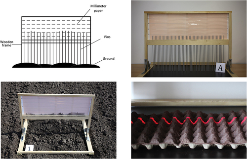
where L₂ is the measured Euclidean distance between the chain ends while on the surface and L₁ is the length of the stretched chain. In our measurements L₂ = 1 m and the chain link pitch is 12.5 mm. The pinboard contact method assumes multiple elevation measurements using a set of equidistant identical pins as depicted in Figure 1. SR is computed as the standard deviation (SD) of the measurements after the elimination of slope effects (Cremers et al., 1996). Usually, classical contact methods are computed on 1 m² areas, in several directions. However, we consider that approaches based on digital imaging are best suited for the estimation of SR, as they are most suited for the analysis of anisotropic surfaces and materials, which is the case of soil. In addition, measuring SR in different directions with classical approaches, followed by averaging, may lead to a misinterpretation of the experimental results (Marandskiy & Ivanovici, 2023). In our in-lab and in-situ experiments, we determined that the pinboard measurements have the smaller error compared to the chain method, therefore we embraced the pinboard method as reference for all our experimentation, comparison and validation.

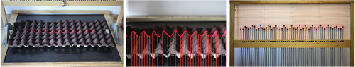
Figure 1. Diagram of pinboard setup (top left), the pinboard calibration on a flat artificial surface (top right), in situ usage (bottom left) and red laser projection for soil profile emphasis on a synthetic surface (bottom right).

In this article, we propose an AI-based approach for soil roughness estimation in digital images acquired with the help of a laser line to enhance the visibility of the soil profile. The research hypothesis is that an AI model is capable of learning, in a supervised way, the correspondence between digital images and SR measurements performed with a classical method (the pinboard in our case). The ultimate goal, which is not the purpose of the current article, is to propose a complete methodology or framework of SR estimation in digital images from a bird’s-eye-view perspective, without the usage of any other additional technology, like the laser line beam.

The optimization in decision-making processes and automated analysis using tools from AI lead to appearance of the fifth-generation agriculture, or, as it is known, AG5.0. In this stage, the key improvement with respect to the fourth generation is the introduction and increased reliance on AI models. Moreover, the AI is offering promising results for data analysis in agriculture, as the Big Data available cannot be processed or analysed using the classical computational paradigms. AI-based solutions are being developed to learn and adapt based on accumulated experience, so that in the future will be able to take automatic actions purely based on data analysis. A detailed perspective on what is AI can be found in (Russell, 2010).

Machine Learning (ML) is a particular type of AI mostly useful when the relation between causality, measurements and, respectively, the decision are not evident. Thus, data is acquired and the trainable system learns the input-output correspondence exemplified during the training process. The classical neural networks, which were milestones in the historical machine learning, evolved into the deep convolutional neural networks (LeCun et al., 1998). Deep networks (Goodfellow et al., 2016) showed their proficiency especially when the input data are images, from RGB to multi- or hyper-spectral ones. In the classical, non-deep model of learning, the features that describe the input images are manually selected and then the classifier is trained. In contrast, in the deep learning model, both the features and the network are jointly approached and have their weights (and contribution) determined automatically in the training process. Compared to their classical multilayer perceptron counterparts, deep convolutional network come with more depth which allows a better structuring of the information, feature which highly increases the efficiency in learning the information available in the training set. Following their won of the ILSVCR competition (Krizhevsky et al., 2012), convolutional neural networks (CNNs) become dominant in computer vision tasks, managing to overcome other learners in all problems where there is plenty of data.

ML was previously used for the estimation of surface roughness, not necessarily soil but other types of surfaces in industry-related applications. For example, in (Palande et al., 2022), the surface roughness was estimated for milled surfaces using a stylus-based instrument and a linear regression model based on digital images. In (Elangovan et al., 2015) the surface roughness is estimated also in a manufacturing context, using a multiple-regression analysis. A similar manufacturing context is presented in (Zhang, 2021). Of particular interest for the agriculture context, soil roughness was estimated deploying ML and various input data. For instance, in (Singh et al., 2021) SR was estimated in satellite images, more specifically synthetic aperture radar images and a pinboard was used to measure SR in the field. In (Herodowicz-Mleczak et al., 2022) the SR is estimated based on a digital elevation model (DEM) which has to be estimated using various techniques, like the stereo-photography or by laser scanning, both of them requiring relatively expensive equipment. Alternatively, an RGB-depth camera could be used to produce a small-scale DEM of the soil surface, like in (Matranga et al., 2023). In (Herodowicz-Mleczak et al., 2023) SR is computed based on proximal measurements of spectral reflectance in the VIS-NIR range, which requires the usage of a spectroradiometer, a high-value equipment.

In this article we use two CNN models for learning the correspondence between digital images and the soil roughness estimates provided by a classical contact method. We use both grey-scale and colour images for the training of the two models, and in both cases the soil profile is highlighted by using a red laser line projected on the soil surface. For training, we created two custom data sets based on both synthetic and real soil samples. We present experimental results, their interpretation and conclude the paper.

Materials and methods

Materials

Our custom-made pinboard has 53 aluminium pins 33 cm in height. The inter-pin gap is ½” = 1.25 cm, identical to the distance between joints of the roller chain. The effective measurement line is 72 cm and the dynamic range for the height measurement is 20 cm (i.e. max. pin variation). The background of the pinboard is of millimetre paper to allow reading the pin’s heights in centimetres. The pinboard is shown in Figure 1, as well as its utilization for in-lab and in-situ measurements. In addition to the pinboard method, we used a red laser line projection on the soil samples, in order to emphasize the soil surface variations in the acquired digital images. The line laser source was placed above and perpendicular to the targeted surface. A Canon 5D Mark II digital camera was used for digital image acquisition, tilted at a 30° angle with respect to the surface horizontal plane.

We performed in-lab measurements on various artificial and real soil surfaces, as the ones depicted in Figure 2. The measurements implied the positioning of the pinboard on top of the soil surface and reading the height of each pin, provided the millimetre paper in the background of the pinboard. For the 53 read values, SR was computed as the standard deviation. The completely flat artificial surface allowed for the measurement error estimation (which is less than 1 mm) and pinboard calibration since its SR has a theoretical 0 value and an actual value very close to 0 for both classical contact methods and the laser line beam results in an approximately straight projected line. The regular artificial surface (plastic) contains regularly placed humps of identical shape. The cvasi-regular artificial surface (painted cardboard for holding eggs) contains regularly-placed humps and dimples larger in scale and with small elevation random variations. The irregular artificial surface (uneven concrete) contains random relatively small elevation variations. For the real soil surface more measurements were performed due to its anisotropic nature. The measured SR values are presented in Table 1. These values were used when performing the supervised training of the CNN models considered in this article.

Figure 2. The four types of artificial and real soil surfaces used for in-lab measurements.

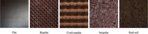
Table 1. The SR values for the synthetic and real soil samples, as measured using the pinboard.

Sample type	Flat	Regular	Cvasi-regular	Irregular	Real soil
SR values	0.094	0.271	1.011, 0.922	0.347	0.826

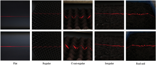
In order to create the data sets for training the AI models, a set of color digital images were acquired for the 5 soil samples. For the emphasis of the soil surface profile, we used a line laser projected on the soil surface. The laser source was placed in the same position as the middle pin, so that the laser beam was perpendicular to the surface and highlighted the same line as previously measured with the pins. The camera was placed on a tripod having the laser projection in the center on the image. The camera was tilted at 30 degrees with respect to the horizontal plane. The distribution of the 28 acquired colour images is 1, 4, 3, 10 and 10 for the flat, regular, cvasi-regular, irregular and real soil surfaces, respectively. From these images, two distinctive data sets were created. For the creation of the first data set, the following sequence of transformations was applied: cropping areas of interest of 1500 × 3000 pixels, scaling to 100 × 200 pixels, binarization and noise addition (Gaussian, speckle, salt and paper) for data augmentation. The result is a data set with 224 images from which 5 samples are depicted in Figure 3, one for each type of surface. For the creation of the second data set, from each original colour 5 5 areas of interest of size 1878 × 1878 pixels were first cropped. In each case, the set of square regions covered the entire length of the laser projection without uncovered areas. The resulting 140 colour images are resized to 256 × 256 pixels. For the augmentation of the training data, the following sequence of transformations is applied to the resulting images: random crop of a 224 × 224 pixels region, 50% chance of horizontal flip, 50% chance of vertical flip, rotation around the image center with a random angle between −5° and 5° and applying a random brightness scaling factor between 0.8 and 1.2. For the validation and testing only a 224 × 224 pixels central region crop is applied (see Figure 4 for illustrations of the resulting image crops).

Figure 3. Sample 100 × 200 pixels areas of interest cropped and scaled from RGB images of the projections of a red laser line beam on the surface samples from Figure 2 (top row), binarized (black and white) images (middle row) and grayscale images derived from the binarized ones by adding Gaussian noise of 0 mean and 1% variance (bottom row).

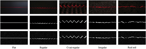
Figure 4. Sample 256 × 256 pixels areas of interest cropped and scaled from RGB images of the projections of a red laser line beam on the surface samples from Figure 2 (top row), random 224 × 224 pixels crops (bottom row) with the following random transformations (from left to right): random brightness scaling, vertical flip, horizontal flip plus random clockwise rotation and random brightness scaling, random clockwise rotation and horizontal flip.

Methods

We employed a machine learning framework. In particular, this framework is based on deep learning and such a model receives at input an image from the dataset and has to predict the value of soil roughness of the said image. We embraced two CNN architectures – VGG-11 (Simonyan & Zisserman, 2015) and ResNet-18 (He et al., 2016). We have chosen these models because they are representative for the two types of connectivity used in deep networks models. These two types are related to the amount of information in the target database. Architecture like VGG (without skip-connections) having their weights pre-trained are to be preferred on databases with limited information since the pre-trained values of the weights offer a very good starting point. In contrast, for databases with more information, networks that use skip-connection to address the problems of vanishing gradients are to be preferred since the skip-connections offer better gradient flow during training, and weights are learned better. Since, before exploring in training-testing, due to unperceived redundancy, one cannot accurately determine the amount of information in a database, selecting one model from each category allows exploring more thoroughly the database. Both models have been tested in a software-only approach, while the former one was chosen as golden model for the hardware implementation (Feldioreanu et al., 2023).

VGG-11

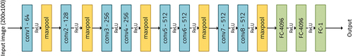
The first CNN model is based on the VGG-11 architecture proposed in (Simonyan & Zisserman, 2015) which has 8 convolutional and 3 fully connected layers. Our model has several modifications such as the input layer size (implicitly this causes changed sizes for all the other layers) and the number of neurons in the last fully connected layer. The VGG models are known to be the largest deep network (i.e with most parameters) that avoids skip-connections. They became popular due to their structured choice for stacking convolutional layers and many parameters involved. Therefore, they are particularly suitable for problems which have limited data, but also do have enough complexity to overcome classical, non-deep, models. Its detailed architecture is depicted in Figure 5. All convolutions use a receptive field of 3 which moves with a stride of 1 while the input 3D volume is zero-padded with 1 pixel. Max-pooling is executed over a 2 × 2 pixels window which moves with a stride of 2.

Figure 5. The architecture of our VGG-11 model.

ResNet-18

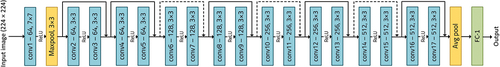
Yet the VGG neural network models, in the last years, became less popular due to limitations introduced by the vanishing gradient problem (He et al., 2016). This issue refers to the exponentially diminishing gradient magnitude with the increase of the numbers of layers in the network (i.e. with depth); a very deep network has very small gradient magnitude in the backpropagation algorithm for the weights in the layers near the input; thus, it requires very large databases and longer training of the model to provide significant corrections in the learning process. This problem noted a significant alleviation within skip-connection (known, here, as residual connection) introduced by He et al. (2016). The skip-connection implements an identity map and allows high magnitude gradient to be injected directly into layers nearer the input. An immediate consequence was that networks become deeper, with more layers but less weights, and, more importantly, with increased performance. Residual networks (Resnet) family contains many models marked by the number of layers used. More recent derivations improve the performance adding aggregated residual transformation (ResNetXt family) (Hu et al., 2018; Xie et al., 2017).

Our CNN model based on the ResNet-18 model architecture proposed in (Xie et al., 2017) which has 17 convolutional layers and only one fully connected layer and is depicted in Figure 6. Our sole modification is the number of neurons of the fully connected layer.

Figure 6. The architecture of our ResNet-18 model.

Results

In this section we present the experimental results we obtained with the two deep convolutional models. The models have been implemented in PyTorch (Paszke et al., 2019).

Results for VGG-11

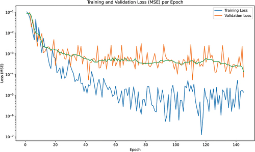
For the training of the VGG-11 we used the first data set comprising 224 grayscale images of 200 × 100pixels. We used 144 images (64.28%) for training, 40 images (17.86%) for validation and 40 images (17.86%) for testing. The VGG-11 was trained for 145 epochs, in a supervised way, using the Stochastic Gradient Descent (SGD) optimizer with a Mean Square Error (MSE) loss function, a momentum of 0.9 and an initial learning rate of 0.021. ReduceLROnPlateau learning rate scheduler with a factor of 0.1 and a patience of 20 was deployed; this means that the loss function value over the training set is monitored, and when it stops improving for a number of “patience” epochs, one assumes that it has reached the minimum within “learning_rate x magnitude_of_loss_gradient” range. To improve, the learning rate is reduced by “factor”, thus diminishing the reachable distance to the minimum of the loss function. The training and validation loss per each epoch are depicted in Figure 7, on a logarithmic scale. The green trace represents the average validation loss for the previous 10 epochs. The CNN yields MSEs of 0.000014, 0.000075 and 0.001651 on the train, validation and test data sets, respectively. On the test set, the mean absolute percentage error (MAPE) (Myttenaere et al., 2016) for the pinboard SR prediction is 5.28% which corresponds to an accuracy of 94.72%. MAPE is calculated as in eq. (2)

(2) $\mathit{MAPE}=\mathit{\hspace{0.17em}}\frac{1}{N}{\sum }_{i=1}^N\left|\frac{P_i-A_i}{A_i}\right|\times 100\mathit{\hspace{0.17em}}\left[\mathrm{\%}\right],$(2)

Figure 7. VGG-11 training and validation loss per epoch (logarithmic vertical scale). The green line represents the moving average computed on an arbitrarily-chosen window size, in order to emphasize the decreasing tendency of the validation loss despite its large variations.

where P_i is the predicted value and A_i is the actual SR value. Preliminary results were reported in (Popa et al., 2023).

Results for ResNet-18

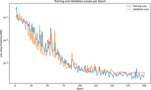
For the training of the ResNet-18 we used the second data set comprising of 140 RGB images of 256 × 256 pixels. We randomly selected 100 images (71.42%) for training, 20 (14.29%) for validation and 20 (14.29%) for testing. The ResNet-18 was trained for 200 epochs, in a supervised way, using the SGD optimizer with an MSE loss function, a momentum of 0.9 and various initial learning rates. Cosine Annealing (Loshchilov & Hutter, 2017) learning rate scheduler with a maximum of 200 iterations was deployed. For an initial learning rate of 0.0005, the CNN yields MSEs of 0.000377, 0.000396 and 0.000217 for the training, validation and test data sets, respectively. On the test set, the MAPE for the pinboard SR prediction is 3.05% which corresponds to an accuracy of 96.95%. The training and validation losses per each epoch are depicted in Figure 8, on a logarithmic scale.

Figure 8. ResNet-18 training and validation loss per epoch (logarithmic vertical scale) for an initial learning rate of 0.0005.

For an initial learning rate of 0.0008, the CNN yields MSEs of 0.005151, 0.003204 and 0.003121 for the training, validation and test data sets, respectively. On the test set, the MAPE for the pinboard SR prediction is 9.29% which corresponds to an accuracy of 90.71%. The training and validation losses per each epoch are depicted in Figure 8, on a logarithmic vertical scale.

In order to summarize the experimental results, we present the MAPE for the pinboard SR prediction and overall accuracy in Table 2. One may note that we obtained better results when using the VGG-11 model, which is considered obsolete in the literature. However, the slightly lower performance of the ResNet-18 model may be due to the small size of the data set used for training and we expect to obtain better results in our future experiments using this particular type of CNN model.

Table 2. The MAPE of pinboard SR prediction and overall accuracy for our experiments with the VGG-11 and ResNet-18 models.

CNN type	VGG-11	ResNet-18
MAPE	5.28%	9.29%
Accuracy	94.72%	90.71%

Discussion

Regarding the difference in performance between VGG-11 and ResNet-18, there are several aspects to be mentioned: the VGG-11 has three fully-connected layers for the last layers, it does not contain skip-connections and the model contains more parameters. ResNet-18 is deeper with less parameters, but gradient injection is optimized due to residual connections. The comparison between the two is in fact a comparison of how much information is actually in the data set and how complex is the process to retrieve the information from the data. A VGG network will behave better for any problems with limited complexity, but multiple corner cases. The larger depth of the ResNet makes it more suitable for more complex problems, but the smaller number of parameters limits the number of corner cases that can be dealt with. The first data set used for VGG-11 is simplified due to the binarization of the input images, thus the model has a simpler job in learning the correspondence between laser-emphasized soil profiles and the soil roughness estimates. The reason for which we choose specifically small models is related to the nature of the convolutional networks: they come with many parameters and, thus, especially for limited data sets, they could be prone to overfitting. To make a better case, we use the augmentation in the testing set, to put the network in face of different views and to have a better estimate of the achievable performance. However, these models, as is typical for any AI model, will carry in the prediction the limitation from annotation in the training set and also may add their own errors. These were experimentally evaluated and the reported top value of MAPE around 10%.

In order to validate our experiments, we tested the equivalence of the SR measured with the pinboard and SR computed from the digital images acquired with the laser projection, on the same line of the cvasi-regular surface. The laser line was projected onto the exactly same line on the surface where the pins of the pinboard were previously placed. The resulted images contained the entire laser projection and a straight, horizontal reference line at the same height as the laser, to enable the SR estimation in the digital images. We measured the distance in pixels from this reference line to the laser projection on the surface for each pin position, as depicted in Figure 9. By normalizing the values in each case (i.e. subtracting the minimum value and dividing the result by the difference between the maximum and minimum values) and computing the standard deviation SD, the resulting values are very close: 0.298 in digital images, with respect to 0.303, thus an absolute error of 0.005 which corresponds to 1.65%. Due to the normalization step, there is no need to adapt the perspective in the acquired digital image.

Figure 9. Testing the equivalence between SR estimation using pinboard measurements and laser-based measurements in the digital image: set-up with pinboard and laser line (left), laser line-based SR estimation (middle) and pinboard SR measurement (right).

A source of error is the usage of pinboard measurements for the training of the two CNNs. We consider that a higher spatial sampling frequency will improve further the laser results and have results closer to reality than the pinboard. Computing SR using the laser line projection will be equivalent to using a very high spatial resolution pinboard and a higher precision. In addition, the usage of the laser allows for a non-invasive measurement, thus avoiding any altering of the soil samples, which is inevitable when using the pinboard. This could be even further improved and simplified in the future, by using for training a better soil roughness estimate computed based on the laser profile directly from the digital images. In that case, the images that will be used for training will no longer contain the laser profile but only the top view of the soil surface.

Conclusion

In this article we proposed the usage of digital image and AI models for the estimation of soil roughness parameter of important relevance for agriculture. We used a red laser line to emphasize the profile of the soil surface and fixed image acquisition conditions (soil sample, pinboard and camera position, angles, illumination, camera settings, etc.). We focused on two AI models, in particular two CNN architectures: VGG-11 and ResNet-18. We produced our own data sets and in-lab validation was performed on both synthetic and real soil samples.

As future work, we envisage further increasing the size of the training data set in order to avoid overfitting and to increase the precision in the estimation of soil roughness. In addition, to perform systematic in-situ measurements for Spring 2024.

The two data sets presented in this article will be made publicly available.

Acknowledgments

This work was funded by the AI4AGRI project entitled “Romanian Excellence Center on Artificial Intelligence on Earth Observation Data for Agriculture”. The AI4AGRI project received funding from the European Union’s Horizon Europe research and innovation program under grant GA no. 101079136.

Disclosure statement

No potential conflict of interest was reported by the author(s).

Additional information

Funding

The work was supported by the European Union [101079136].

References

- Aguilar, M., Aguilar, F., & Negreiros, J. (2009). Off-the-shelf laser scanning and close-range digital photogrammetry for measuring agricultural soils microrelief. Biosystems Engineering, 103(4), 504–11. https://doi.org/10.1016/j.biosystemseng.2009.02.010
- Al-Kaisi, M. M., Lal, R., Olson, K. R., & Lowery, B. (2017). Chapter 1 - fundamentals and functions of soil environment. In M. Mahdi & B.L. Al-Kaisi (Eds.), Soil health and intensification of agroecosytems (pp. 1–23). Academic Press.
- Allmaras, R. R., Burwell, R. E., Larson, W. E., & Holt, R. F. (1966). Total porosity and random roughness of the interrow zone as influenced by tillage, agricultural research service. US Dept. of Agriculture.
- Amoah, J. K. O., Amatya, D. M., & Nnaji, S. (2013). Quantifying watershed surface depression storage: Determination and application in a hydrologic model. Hydrological Processes, 274(17), 2401–2413. https://doi.org/10.1002/hyp.9364
- Barneveld, R. J., Seeger, M., & Maalen-Johansen, I. (2013). Assessment of terrestrial laser scanning technology for obtaining high-resolution DEMs of soils. Earth Surface Processes and Landforms, 38(1), 90–94. https://doi.org/10.1002/esp.3344
- Boegh, E., Soegaard, H., Broge, N., Hasager, C. B., Jensen, N. O., Schelde, K., & Thomsen, A. (2002). Airborne multispectral data for quantifying leaf area index, nitrogen concentration, and photosynthetic efficiency in agriculture. Remote Sensing of Environment, 81(2–3), 179–193. https://doi.org/10.1016/S0034-4257(01)00342-X
- Burwell, R. E., Allmaras, R. R., & Amemiya, M. (1963). A field measurement of total porosity and surface microrelief of soils. Soil Science Society of America Journal, 27(6), 697–700. https://doi.org/10.2136/sssaj1963.03615995002700060037x
- Connolly, A. (2022). 10 Digital Technologies That Are Transforming Agriculture. https://www.forbes.com/sites/forbestechcouncil/2022/04/26/10-digital-technologies-that-are-transforming-agriculture
- Cremers, N. H. D. T., Van Dijk, P. M., De Roo, A. P. J., & Verzandvoort, M. A. (1996). Spatial and temporal variability of soil surface roughness and the application in hydrological and soil erosion modelling. Hydrological Processes, 10(8), 1035–1047.
- Elangovan, M., Sakthivel, N. R., Saravanamurugan, S., Nair, B. B., & Sugumaran, V. (2015). Machine learning approach to the prediction of surface roughness using statistical features of vibration signal acquired in turning. Procedia Computer Science, 50, 282–288. https://doi.org/10.1016/j.procs.2015.04.047
- Feldioreanu, G., Popa, S., & Ivanovici, M. (2023). Convolutional neural network implemented on FPGA for trajectory classification. International Symposium on Signals, Circuits and Systems (ISSCS) (pp. 1–4). Iasi, Romania.
- Goodfellow, I., Bengio, Y., & Courville, A. (2016). Deep learning. MIT press.
- Herodowicz-Mleczak, K., Piekarczyk, J., Kaźmierowski, C., Nowosad, J., & Mleczak, M. (2022). Estimating soil surface roughness with models based on the information about tillage practises and soil parameters. Journal of Advances in Modeling Earth Systems, 14(3). https://doi.org/10.1029/2021MS002578
- Herodowicz-Mleczak, K., Piekarczyk, J., Ratajkiewicz, H., Nowosad, J., Śledź, S., Kaźmierowski, C., Królewicz, S., & Kierzek, R. (2023). Estimation of soil surface roughness parameters under simulated rainfall using spectral reflectance in optical domain. Earth & Space Science, 10(8). https://doi.org/10.1029/2022EA002642
- Herodowicz, K., & Piekarczyk, J. (2018). Effects of soil surface roughness on soil processes and remote sensing data interpretation and its measuring techniques - a review. Polish Journal of Soil Science, 51(2), 229. https://doi.org/10.17951/pjss.2018.51.2.229
- He, K., Zhang, X., Ren, S., & Sun, J. (2016). Deep residual learning for image recognition. In Proceedings of the IEEE conference on computer vision and pattern recognition, Las Vegas, NV, USA (pp. 770–778).
- Hu, J., Shen, L., & Sun, G. (2018). Squeeze-and-excitation networks. In Proceedings of the IEEE conference on computer vision and pattern recognition, Salt Lake City, UT, USA (pp. 7132–7141).
- Krizhevsky, A., Sutskever, I., & Hinton, G. E. (2012). ImageNet classification with deep convolutional neural networks. In Proceedings of the 25th International Conference on Neural Information Processing Systems, Lake Tahoe, NV, (Vol. 25, pp. 1097–1105). https://dl.acm.org/doi/10.1145/3065386
- Latief, A., & Firasath, N. (2021). Agriculture 5.0: Artificial Intelligence, IoT and machine learning. CRC Press.
- LeCun, Y., Bottou, L., Bengio, Y., & Haffner, P. (1998). Gradient-based learning applied to document recognition. Proceedings of the IEEE, 86(11), 2278–2324. https://doi.org/10.1109/5.726791
- Loshchilov, I., & Hutter, F. (2017). SGDR: Stochastic Gradient Descent with Warm Restarts. In International Conference on Learning Representations, Toulon, France.
- Mankoff, K. D., & Russo, T. A. (2013). The kinect: A low-cost, high-resolution, short-range 3D camera. Earth Surface Processes and Landforms, 38(9), 926–936. https://doi.org/10.1002/esp.3332
- Marandskiy, K., & Ivanovici, M. (2023, July 13–14). Soil roughness estimation using fractal analysis on digital images of soil surface. International Symposium on Signals, Circuits and Systems, Iasi, Romania.
- Matranga, G., Palazzi, F., Leanza, A., Milella, A., Reina, G., Cavallo, E., & Biddoccu, M. (2023). Estimating soil surface roughness by proximal sensing for soil erosion modeling implementation at field scale. Environmental Research, 238(2), 117191. https://doi.org/10.1016/j.envres.2023.117191
- Moreno, R. G., Diaz Alvarez, M. C., Tarquis, A., Gonzalez, A. P., & Requejo, A. S. (2010). Shadow analysis of soil surface roughness compared to the chain set method and direct measurement of micro-relief. Biogeosciences, 7(8), 2477–2487. https://doi.org/10.5194/bg-7-2477-2010
- Morgan, R. P. C., & Duzant, J. H. (2008). Modified MMF (Morgan–Morgan–Finney) model for evaluating effects of crops and vegetation cover on soil erosion. Earth Surface Processes and Landforms, 33(1), 90–106. https://doi.org/10.1002/esp.1530
- Morris, J. B., & Wang, M. L. (2007). Anthocyanin and potential therapeutic traits in clitoria, desmodium, catharanthus and hibiscus species acta hort. ISHS.
- Myttenaere, A. D., Golden, B., Le Grand, B., & Rossi, F. (2016). Mean Absolute Percentage Error for Regression Models. Neurocomputing, 192(June), 38–48. https://doi.org/10.1016/j.neucom.2015.12.114
- Palande, C., Nadar, R., Ambadekar, P., Sridhar, K., & Vashistha, T. (2022). Machine learning application for prediction of surface roughness of milled surface. In S. Kumar, J. Ramkumar, & P. Kyratsis (Eds.), Recent advances in manufacturing modelling and optimization. lecture notes in mechanical engineering (pp. 203–219). Springer.
- Paszke, A., Gross, S., Massa, F., Lerer, A., Bradbury, J., Chanan, G., Killeen, T., Lin, Z., Gimelshein, N., Antiga, L., & Desmaison, A. (2019). PyTorch: An imperative style, high-performance deep learning library. Advances in Neural Information Processing Systems, 32, 8024–8035. https://doi.org/10.48550/arXiv.1912.01703
- Popa, S., Feldioreanu, G., Marandskiy, K., & Ivanovici, M. (2023, July 3–6). Convolutional Neural Network Hardware Implementation for Soil Roughness Estimation 42nd EARSeL Symposium, Bucuresti, Romania.
- Prasannakumar, V., Vijith, H., Abinod, S., & Geetha, N. (2012). Estimation of soil erosion risk within a small mountainous sub-watershed in Kerala, India, using Revised Universal Soil Loss Equation (RUSLE) and geo-information technology. Geoscience Frontiers, 3(2), 209–215. https://doi.org/10.1016/j.gsf.2011.11.003
- Rouse, J., Haas, R., & Schell, J. (1973). Monitoring vegetation systems in the Great Plains with ERTS, NASA Spec. Publication, 309–317. https://ntrs.nasa.gov/citations/19740022614
- Russell, S. J. (2010). Artificial intelligence a modern approach. Pearson Education, Inc.
- Saleh, A. (1993). Soil roughness measurement: Chain method. Journal of Soil and Water Conservation, 48(6), 527–529.
- Sasidharan, T. S., Latini, D., Ivanovici, M., Schiavon, G., Thangavel, K., & Del Frate, F. (2023, July 3–6). Smart weed control: Real-time inference and on-board data processing using edge-AI. EARSeL Symposium, Bucharest, Romania.
- Shapiro, C. A., Schepers, J. S., Francis, D. D., & Shanahan, J. F. (2013). Using a chlorophyll meter to improve N management. University of Nebraska-Lincoln Extension, Institute of Agriculture and Natural Resources.
- Simonyan, K., & Zisserman, A. (2015). Very deep convolutional networks for large-scale image recognition. In Proceedings of the 3rd International Conference on Learning Representations, Computational and Biological Learning Society, Boston, MA, USA (pp. 1–14).
- Singh, A., Gaurav, K., Rai, A. K., & Beg, Z. (2021). Machine learning to estimate surface roughness from Satellite Images. Remote Sensing, 3(19), 3794. https://doi.org/10.3390/rs13193794
- Skierucha, W., Wilczek, A., Szypłowska, A., Sławiński, C., & Lamorski, K. (2012). A TDR-Based soil moisture monitoring system with simultaneous measurement of soil temperature and electrical conductivity. Sensors, 12(10), 13545–13566. https://doi.org/10.3390/s121013545
- Thomsen, L., Baartman, J., Barneveld, R., Starkloff, T., & Stolte, J. (2015). Soil surface roughness: Comparing old and new measuring methods and application in a soil erosion model. Soil, 1(1), 399–410. https://doi.org/10.5194/soil-1-399-2015
- Vidal Vázquez, E., Vivas Miranda, J. G., & Paz González, A. (2005). Characterizing anisotropy and heterogeneity of soil surface microtopography using fractal models. Ecological Modelling, 182(3–4), 337–353. https://doi.org/10.1016/j.ecolmodel.2004.04.012
- Xie, S., Girshick, R., Dollár, P., Tu, Z., & He, K. (2017). Aggregated residual transformations for deep neural networks. In Proceedings of the IEEE conference on computer vision and pattern recognition, Honolulu, HI, USA (pp. 1492–1500). https://doi.org/10.1109/CVPR.2017.634
- Zhang, W. (2021, February 26–28). Surface roughness prediction with machine learning. Journal of Physics: Conference Series, 1856, International Conference on Computer Network Security and Software Engineering (CNSSE 2021), Zhuhai, China.