Feasibility of proton dosimetry overriding planning CT with daily CBCT elaborated through generative artificial intelligence tools

Abstract

Radiotherapy commonly utilizes cone beam computed tomography (CBCT) for patient positioning and treatment monitoring. CBCT is deemed to be secure for patients, making it suitable for the delivery of fractional doses. However, limitations such as a narrow field of view, beam hardening, scattered radiation artifacts, and variability in pixel intensity hinder the direct use of raw CBCT for dose recalculation during treatment. To address this issue, reliable correction techniques are necessary to remove artifacts and remap pixel intensity into Hounsfield Units (HU) values. This study proposes a deep-learning framework for calibrating CBCT images acquired with narrow field of view (FOV) systems and demonstrates its potential use in proton treatment planning updates. Cycle-consistent generative adversarial networks (cGAN) processes raw CBCT to reduce scatter and remap HU. Monte Carlo simulation is used to generate CBCT scans, enabling the possibility to focus solely on the algorithm’s ability to reduce artifacts and cupping effects without considering intra-patient longitudinal variability and producing a fair comparison between planning CT (pCT) and calibrated CBCT dosimetry. To showcase the viability of the approach using real-world data, experiments were also conducted using real CBCT. Tests were performed on a publicly available dataset of 40 patients who received ablative radiation therapy for pancreatic cancer. The simulated CBCT calibration led to a difference in proton dosimetry of less than 2%, compared to the planning CT. The potential toxicity effect on the organs at risk decreased from about 50% (uncalibrated) up the 2% (calibrated). The gamma pass rate at 3%/2 mm produced an improvement of about 37% in replicating the prescribed dose before and after calibration (53.78% vs 90.26%). Real data also confirmed this with slightly inferior performances for the same criteria (65.36% vs 87.20%). These results may confirm that generative artificial intelligence brings the use of narrow FOV CBCT scans incrementally closer to clinical translation in proton therapy planning updates.

Keywords:

• Deep learning
• image-to-image translation
• dosimetry
• cycleGAN
• CBCT
• CT
• limited FOV
• artifact correction
• hounsfield unit recovery

1. Introduction

Medical imaging plays a crucial role in oncology, particularly in radiotherapy. Computed tomography (CT) is the primary modality used in radiation therapy for high-resolution patient geometry and accurate dose calculations [1]. However, CT is associated with high patient exposure to ionizing radiation. Cone-beam computed tomography (CBCT) has the potential to provide faster imaging and reduce patient exposure to non-therapeutic radiation. This makes it a valuable imaging modality used for patient positioning and monitoring in radiotherapy. CBCT is currently used to monitor and detect changes in patient anatomy throughout the treatment. It is also compatible with fractional dose delivery, making it a patient-safe imaging modality with less additional non-therapeutic dose than traditional CT. However, this modality can introduce scattered radiation image artifacts like shading, cupping, and beam-hardening [2,3]. The artifacts resulting from scattered radiation in CBCT images can cause fluctuations in pixel values, making it difficult to use these images directly for dose calculation. Consequently, CBCT images cannot be used directly for dose calculations unless correction methods are applied. Reliable correction techniques for calibrating CBCT images to Hounsfield Unit (HU) values used by CT scanners would expand the clinical usage of CBCT in treatment planning and evaluation of tumor shrinkage and organ shift [4–6]. In recent years, traditional approaches, such as anti-scatter grid, partial beam blockers, and scattering estimators [7–9], have been joined to deep learning-based methods, which have been showing interesting potential to improve CBCT quality [10]. Such methods, leveraging mainly convolutional neural networks (CNN) and generative adversarial networks (GAN), were investigated to map the physical model of the x-ray interaction with matter disregarding the underlying complex analytics and avoiding the use of explicit statistical approaches such as Monte Carlo. Aiming at removing scatter and correcting HU units in CBCT scans, many authors explored various types of CNN, ranging from UNet trained with a supervised training approach [11–15] to the more complex cycle-consistent Generative Adversarial Network (cGAN), based on an unsupervised training approach [16–21]. cGAN model consists of two subnetworks, the generator and the discriminator, with opposite roles. While the generator tries to learn how to convert one dataset to another, the discriminator distinguishes between real and synthetic images. This process creates a cycle-consistent loop that improves the generator’s ability to produce synthetic images that look just like real ones. Focusing on CBCT-to-CT mapping, Xie et al. proposed a scatter artifact removal CNN based on a contextual loss function trained on the pelvis region of 11 subjects to correct the CBCT artifacts in the pelvic area [22]. Another research focused on a cGAN model to calibrate CBCT HU values in the pelvis region. The model was trained on 49 patients with unpaired data and tested on nine independent subjects, and the authors claimed the method kept the anatomical structure of CBCT images unchanged [18]. Exploring the use of deep residual neural networks in this field, a study demonstrated the capability of such architectures by proposing an iterative tuning-based training, where images with increasing resolutions are used at each step [23]. Likewise, our group recently reported that cGAN has better capability than CNN trained with pure supervised techniques to preserve anatomical coherence [24]. All these contributions, however, did not address the consistency of the treatment planning performed with the corrected CBCT. Conversely, Zhang et al. [25] reported the test of pelvis treatment planning in proton therapy performed on CBCT corrected with CNN. However, they summarized that the dose distribution calculated for traditional photon-based treatment outperformed the one computed for proton therapy. CBCT corrected with a cGAN was applied to evaluate the quality of the proton therapy planning in cancer treatment across different datasets with satisfactory results [13,20]. All the mentioned research works focused on the problem of CBCT-to-CT HU conversion exploiting CBCT with a wide field of view (FOV). However, some systems present in clinical practice have a limited FOV, not sufficient to contain the entire volume of the patient, e.g. in the presence of large regions such as the pelvis or with obese patients [26]. Considering the current use of CBCT for patient positioning purposes, small FOV CBCT systems could be preferred due to their reduced imaging dose, shorter computation time, and increased resolution over the treatment region of interest [27]. However, the limited FOV also causes a truncation problem during reconstruction [28,29]. Consequently, the non-uniqueness of the solution for the iterative reconstruction causes additional bright-band effects that add artifacts to the CBCT [30]. Even in the case of optimal HU calibration and scatter reduction, a CBCT, acquired in a narrow FOV cannot be used for adaptive dose planning. Especially, narrow FOV CBCT lacks important anatomical information (e.g. the air/skin interface) necessary for properly calculating the beam path. The present work aimed to propose a deep-learning framework that elaborates the CBCT to calibrate the HU, remove artifacts due to the conic geometry acquisition, and handle narrow FOV issues to demonstrate the potential use of the corrected CBCT in the context of proton treatment planning updates. The work is part of a larger study carried out in collaboration with the Italian National Center of Hadrontherapy (CNAO, Pavia, Italy) that aims to explore the possibility of using the in-house narrow FOV CBCT system not only for patient positioning but also for dosimetric evaluation without hardware modifications [31]. The deep-learning framework took its root from the CBCT-to-CT mapping model based on cGAN proposed in [24] that was here extended to address the case of narrow FOV. Tests were carried out on a public dataset of planning CT (pCT) scans of 40 oncological patients affected by pancreatic cancer. In a first attempt, synthetic raw CBCT volumes were properly generated from CT scans throughout the Monte Carlo simulation. This enabled us to dump anatomical variations usually present in real CBCT with respect to the corresponding planning CT. Moreover, in order to demonstrate the feasibility of the methodology also with real data, we replicated each experiment with the clinical CBCT included within the dataset. As the dataset provided annotation data about the segmented lesion and organs at risk, particle beam dosimetry was computed in the original planning CT and the corrected CBCT volume, verifying the coherency between the two dose distributions. The main contributions of this paper may therefore be summarized as:

• capability of the cGAN to correct CBCT (scatter reduction and HU remapping) when applied to small FOV;

• consistency of the proton dosimetry computed on corrected CBCT with respect to the original planning CT.

2. Materials and methods

2.1. Dataset description

A publicly available dataset obtained from the Cancer Imaging Archive, called Pancreatic-CT-CBCT-SEG [32], was exploited in this work. The dataset contained CT acquisition from 40 patients who received ablative radiation therapy for locally advanced pancreatic cancer at Memorial Sloan Kettering Cancer Center. Each CT was acquired during a deep inspiration breath-hold verified with an external respiratory monitor. The dataset al.so included manual segmentations of a region of interest (ROI), defined by expanding the dose planning target volume by 1 cm. Along with the ROI, each scan provided contours of some organ at risk (OAR), namely: (i) the stomach with the first two segments of the duodenum, (ii) the remainder of the small bowel, and (iii) both lungs. The authors reported that the segmentations were performed independently by six radiation oncologists and reviewed by two trained medical physicists. The dataset al.so provided two CBCT scans for each subject. In the first phase, these CBCTs were not considered because they were obtained at different times with respect to the corresponding CT scan, which could lead to potential changes in patient anatomy between acquisitions. Simulated CBCT scans were considered instead by generating them directly from the corresponding planning CT (implementation is detailed below in section 2.1.1). This way, perfect alignment and anatomical correspondence between the two volumes were both ensured, avoiding the need for additional registration steps (rigid or deformable). To summarize, using simulated CBCT scans allowed the study to focus solely on the algorithm’s ability to reduce artifacts and cupping effects without considering intra-patient longitudinal variability. Each experiment was then also replicated with the real small FOV (250 mm diameter) CBCT provided with the dataset by adding an intermediate rigid registration step in the pipeline, in order to demonstrate the feasibility of the methodology also with data from the real world.

2.1.1. CBCT simulation

Synthetic CBCTs were generated from the original available CTs following the approach documented in [33] and replicating the setup and the geometry of CNAO’s CBCT acquisition system [31]. Specifically, Monte Carlo (MC) simulations were conducted to generate primary (P_MC) and scatter (S_MC) X-ray images for each CT scan. All simulations were performed using the GATE open-source software v9.2 (based on Geant4 v11) [34] with fixed forced detection, a variance reduction technique aimed at minimizing computation time. The energy-dependent detector efficiency was based on the design specifications provided by the manufacturer for the Paxscan 4030D (Varian Medical System, Palo Alto, CA). The X-ray fluence spectrum was computed using the open-source software SpekPy [35], employing 3.2 mm Al filtration at 100 kVp. The A-277 X-ray tube (Varian Medical System, Palo Alto, CA), chosen for this work, features a 7${}^{°}$ rhenium-tungsten molybdenum target. Images were produced according to a CBCT scan of ${220}^{°}$ and with projection matching the size of the Paxscan 4030D detector (isometric pixel spacing 0.388 mm, detector size 768 × 1024 pixels). The source-to-detector and source-to-isocenter distances were set to 1600 mm and 1100 mm, respectively. A further acceleration of scatter calculation was achieved by downsampling resolution 8-fold and simulating S_MC at $5^{°}$ steps with a statistical uncertainty $<5\%$. S_MC images were then upsampled and interpolated at the required points to match the corresponding P_MC images. Lastly, the final projections $S_{\mathit{\text{MC}}}+P_{\mathit{\text{MC}}}$ were normalized by the simulated flat field image. 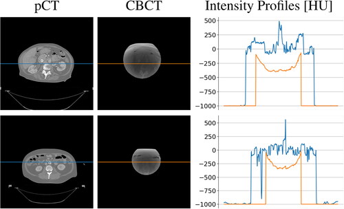CBCT scans were then reconstructed using open-source software RTK [36] at a $1\times 1\times 1$ mm resolution, with a $220\times 220\times 220$ size in pixel and masked to the axial field-of-view of diameter equal to 204 mm. Some examples of planning CT and simulated CBCT axial slices are visible in Figure 1, along with the intensity profile of the central pixel row. The cupping effect is evident as a shaded portion in the middle of the CBCT and confirmed by the concavity in the intensity profile.

Figure 1. Examples of two CT axial slices with their corresponding simulated CBCT. The intensity profiles of the central row (marked as a line in both images) are plotted in the right panel. Each image is displayed with Window = 1300, Level = 0.

2.2. CBCT-to-CT correction

2.2.1. Neural network architecture and main processing layers

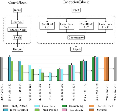
The network implemented for CBCT correction was based on the cycle Generative Adversarial Network (cGAN) [37]. This architecture is based on four concurrent subnetworks, two generators and two discriminators, which work in opposition. While the generators try to learn the mapping to convert CBCT to CT (or CT to CBCT), the discriminator’s objective is to distinguish between authentic and network-generated images. This generator-discriminator cycle-consistent loop is designed to improve the generators’ ability to produce synthetic images that reproduce with high fidelity the characteristic of the destination modality (e.g. generate a calibrated synthetic CT starting from a scattered CBCT). The network’s fundamental processing unit was referred to as ConvBlocks (Figure 2), which were built using a 2D convolution with a 3 × 3 kernel, followed by an instance normalization layer and a swish activation function. Instance normalization was demonstrated to improve the performance in image generation tasks [38]. The use of swish activation was shown to combine the advantages of rectilinear and sigmoid activations. It has a smooth, differentiable form due to the sigmoid component, which can help with training stability and gradient flow [39]. The other basic processing unit for cGAN structure was the InceptionBlock, consisting of four parallel ConvBlocks, each with an increasing kernel size of dimensions 1 × 1, 3 × 3, 7 × 7, and 11 × 11, which processed the same input simultaneously with multiple receptive fields. The output of each branch of InceptionBlock was then combined, and the complete set of feature maps was produced as output. The primary objective of this processing block was to execute multi-scale feature extraction from the initial image. The extracted multi-scale features, varying from small to large receptive fields, can produce improved outcomes for image synthesis. The general design of the generator was then carried out as a modified version of the commonly used U-Net architecture. The U-Net model is usually utilized for solving pixel-by-pixel classification challenges in image segmentation [40]. Still, it can also be used to solve image-to-image conversion problems with minor changes. The overall generator structure, depicted in Figure 2, was composed of a contracting and an expanding path. The upper two processing layers of the generator were based on InceptionBlocks, while the deeper two exploited ConvBlocks. Consequently, the network can be broadly top-bottom divided into two segments, each serving distinct functions: (i) the inception part (upper layers) extracted global contextual information, whereas (ii) the traditional 2D convolution part (bottom layers) was responsible for capturing more intricate context and precise localization. On the other hand, the CNN utilized as the discriminator was responsible for image classification and relied on the PatchGAN architecture [41]. Its architecture was based on four sequential ConvBlocks, each with a kernel size of 4 × 4. In the initial three ConvBlocks, the convolution was set with stride 2, leading to an output tensor with half the size and twice the features map. In contrast, the last ConvBlock had stride one and maintained the size and the number of feature maps unchanged. A sigmoid activation function was applied to the last layer, generating a 32 × 32 map used to classify the input image as real or fake.

Figure 2. Schematic of the Generator model architecture.

2.2.2. Model training

As formerly stated, the cGAN overall training routine employed two generators and two discriminators, competing against one another to solve the CBCT-to-CT conversion problem. The subnetworks were referred to as generator CT (G_CT), generator CBCT (G_CBCT), discriminator CT (D_CT), and discriminator CBCT (D_CBCT). G_CT and G_CBCT were used to produce generated CT from CBCT, and generated CBCT from CT, respectively, while D_CT and D_CBCT were used to distinguish the original CT and CBCT from their generated counterparts. The training routine was subdivided into two main steps occurring simultaneously. In the first step, called the generative phase, G_CT (G_CBCT) took a 2D axial slice of a CBCT (CT) as input and produced a generated CT (generated CBCT) as output. Then, G_CT (G_CBCT) took the generated CT (generated CBCT) as input and produced a cyclic CBCT (cyclic CT), which was supposed to be equal to the original CBCT (CT). At the same time, during the second step, called the classification phase, D_CT (D_CBCT) tried to distinguish between real CT (CBCT) and generated CT (generated CBCT). The whole dataset, consisting of the generated CBCT-pCT (paired) was divided into training, validation, and test sets in proportions of 70%, 15%, and 15%, containing 5698, 1221, and 1221 2D axial slices, respectively. As far as the loss functions are concerned, the generator loss functions included three types of terms, namely adversarial loss, cycle consistency loss, and identity loss. The discriminator loss was composed only of an adversarial term. Further technical details about the network training and implementation can be found in a previous work of our group [24]. The entire cGAN was implemented in Python, using Keras [42] and TensorFlow [43] frameworks.

2.2.3. Performance metrics for model evaluation

The network performances were quantitatively evaluated using the original CT as the ground truth reference. In particular, the metrics evaluated were: (i) peak signal-to-noise ratio (PSNR), (ii) structural similarity index measure (SSIM), and iii) mean absolute error (MAE) [44]. The PSNR quantifies the quality of images by comparing the mean square error of the images being compared to the maximum possible signal power [45]. It is measured in decibels, and its value increases toward infinity as the difference between the calibrated CBCT and ground-truth CT decreases. Therefore, a larger PSNR value indicates better image quality, while a lower value indicates the opposite. SSIM evaluates the resemblance between two images by analyzing their luminance, contrast, and structure [46]. Compared to PSNR, SSIM is considered a more human-like measure of similarity. The SSIM score ranges from 0 to 1, with a value of 1 indicating the highest level of similarity between the images. MAE was used to quantitatively assess the accuracy of Hounsfield Units between the generated CBCT and the original CT. The lower value corresponds to the higher level of HU accuracy between the two images. The significance (p < 0.05) of the statistical difference between CBCT slices prior to and following calibration was verified using Kruskal-Wallis non-parametric test.

2.2.4. Synthetic CT generation pipeline

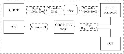
Despite the better quality of calibrated CBCT in terms of HU density values, these volumes cannot yet be used for adaptive dose planning due to their limited FOV. In fact, these CBCT acquisitions lack important anatomical information (e.g. the air/skin interface) necessary for the correct calculation of the beam path. In order to overcome this intrinsic limit, the original planning CT was used to provide the missing information. Therefore, synthetic CT (sCT) is defined in this work as an updated version of the original planning CT overridden with the calibrated voxels from daily CBCT acquired during the treatment. Starting from a scattered CBCT, the following procedure was followed in an axial slice-by-slice approach. At first, each pixel in the slice was clipped between values [–1000; 3000] and then normalized in the [0; 1] range. This step is fundamental because the neural network needs value in this range to operate properly. Then, the generator G_CT processed the normalized CBCT, producing a corrected version of the same axial slice. It is important to remember that G_CT is the only cGAN subnetwork used after completing the training. After neural network processing, the previous pixel clipping guarantees that the normalization can be reversed back to HU. A rigid registration step between the corrected CBCT and the pCT followed, in order to increase the anatomical correspondence. This was based on the SimpleITK registration framework. The process involved optimizing six degrees of freedom, which included three translational and three rotational parameters. Mutual information was used as the similarity metric to quantify the correspondence between intensity patterns in the two images, guiding the optimization algorithm to find the optimal transformation that aligns the CBCT to the pCT in a rigid manner. The result was a registered transformation that improved the spatial alignment of the CBCT and pCT volumes by accounting only for translations and rotations without any other deformation in order to avoid introducing biases in the subsequent operations. This step was applied just for real CBCT, since the generated ones already matched the corresponding pCT anatomy. The last step involved overriding the planning CT pixels with the region acquired with the cone beam modality. Every pixel outside the CBCT FOV belonged to the original CT. The entire pipeline is summarized in Figure 3. In order to evaluate the effective improvement obtained by the corrected CBCT in terms of treatment planning, two versions of sCT were generated for each subject. The first, called sCT corrected (sCTc) was obtained following the mentioned procedure, while the second, called sCT uncorrected (sCTu), was obtained simply by overriding the original CBCT volume without any kind of processing.

Figure 3. Schematic of sCT generation pipeline. *Rigid registration step is applied only to real CBCT scans since generated ones are intrinsically perfectly aligned.

2.3. Dosimetric analysis

2.3.1. Proton-based treatment planning

The treatment plan for each subject was computed with the matRad package [47], an open-source radiation treatment planning toolkit written in Matlab. In particular, the planning was developed using protons as the radiation mode and optimized using the constant relative biological effectiveness times dose method, which accounts for the varying biological effectiveness of different radiation types and energies. A total of 30 fractions were scheduled for the treatment, with two beams used at gantry angles of 0 degrees (anterior direction) and 270 degrees (right lateral direction). Several constraints were chosen in the planning definition to ensure the safety and efficacy of the treatment. For the bowel and stomach regions, squared overdosing and maximum dose volume histogram constraints were used to limit the radiation dose received by these sensitive areas. The lung regions were also subject to squared overdosing constraints to limit the dose delivered to those areas. Finally, the ROI was subject to squared deviation constraints, which aim to keep the dose distribution as close as possible to the prescribed dose (30 fractions of 2 Gy equivalent) [48]. The reference dose planning was first computed directly on the pCT and used as the ground truth in further comparison. Then, this reference plan was updated, giving either corrected or uncorrected sCT as the new volume.

2.3.2. Dose evaluation

To evaluate the suitability of corrected CBCT scans, various metrics were used, including dose difference pass rate (DPR), dose–volume histogram (DVH) metrics, and Gamma pass rates (GPR). The treatment dose computed for the original planning CT was considered as the prescribed ground truth dose [44]. DPR measures the percentage of pixels that meet a certain dose difference threshold, DVH compares cumulative dose to different structures in relation to volume, while GPR assesses the similarity of two dose distributions based on dose difference and distance-to-agreement criteria. The significance (p < 0.05) of the statistical difference in GPR distributions between sCTu and sCTc was verified using the Kruskal-Wallis non-parametric test. Mean doses, D5, and D95, measured on ROI, bowel, and stomach were considered to assess the treatment quality and the toxicity control on the organ at risk.

3. Results

3.1. Qualitative evaluation of the image translation

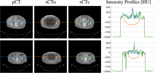
At a qualitative inspection, it can be seen that the darker region clearly visible in the original CBCT due to the cupping artifacts was no longer noticeable after cGAN correction (Figure 4). Likewise, the corrected overwritten sCT scans were more similar to pCTs with respect to their uncorrected counterpart. (Figure 5). Intensity profiles also confirmed this, showing that the concave shape observable in the unprocessed lines disappeared in the processed ones, now matching the HU values range of the reference pCT. This also confirmed that the non-linearity present in the CBCT tissue density was corrected.

Figure 4. Example a CBCT axial slice before (left) and after (right) cGAN correction. As it can be noticed, the cGAN was effective in the correction of the CBCT. Each image is displayed with Window = 1300, Level = 0.

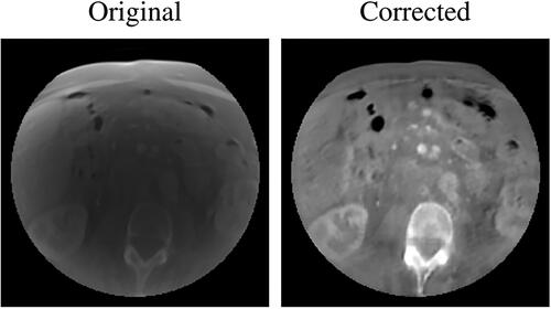
Figure 5. Examples of two CT axial slices with their corresponding sCT generated overriding the uncorrected simulated CBCT (sCTu) and the corrected ones (sCTc). The intensity profiles of the central row (marked as a line in both images) are plotted in the right panel. Each image is displayed with Window = 1300, Level = 0.

3.2. Quantitative evaluation of the image translation

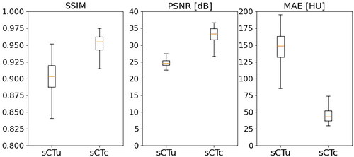
The results from evaluating the model’s performance metrics (Figure 6) showed promising improvements in the quality of the CBCT slices. The original images had a median PSNR of 24.60 dB with an interquartile range (IQR) of 1.40 dB. On the other hand, the processed images had a median PSNR of 33.41 dB (IQR 3.36 dB), resulting in a relative gain of approximately 37%. In terms of the SSIM score, the original images had a median of 0.90 (IQR 0.03), and the processed CBCTs showed a median of 0.95 (IQR 0.02), which corresponded to a relative enhancement of around 5%. Furthermore, the median MAE for the original images was 148.96 HU (IQR 31.24 HU), whereas the median MAE for the processed images was 43.47 HU (IQR 14.82 HU). These results demonstrate the effectiveness of the cGAN approach in improving CBCT image quality. For all three metrics, a statistical difference was found (p < 0.01).

Figure 6. Performance metrics for cGAN model evaluation, computed on the axial slices of the test set before and after model processing.

3.3. Treatment planning evaluation – simulated data

The qualitative comparison between the treatment plans computed for each modality confirmed an ameliorated similarity between sCTc and pCT with respect to their uncorrected counterpart. An example of this can be seen in Figure 7 upper row. It is visible how the beam path computed on sCTu exceeded the ROI releasing a more significant amount of dose in the following tissues. Moreover, it could also be seen that high dose values (red pixels) break over ROI boundaries, indicating that a portion of surrounding healthy areas received overexposure to radiation. This was also confirmed by the dose difference computed with respect to the pCT reference plan (cfr. Figure 7 bottom row). Conversely, the sCTc treatment plan corrected that pattern, showing a more similar beam path and a reduced difference with respect to the pCT plan. Likewise, the dose-volume histogram computed for the same test subject confirmed and enforced such a consideration (Figure 8). Observing the ROI lines, the sCTc (orange dotted line) followed the profile of pCT (orange solid line) more closely than the sCTu (orange dashed line). The treatment plan calculated on sCTc and pCT showed a steep slope, indicating that 2 Gy was the dose delivered to almost all the ROI, while sCTu showed a smoother slope, a sign of overdosing in a portion of this area. Concerning the organs at risk (green and light blue lines), this consideration was even more evident, with an overdosing in the order of about two times with respect to the reference plan. This result would be incompatible with clinical practice. The GPR results for the entire dataset were computed for different gamma criteria and summarized in Table 1 as median (IQR). The median gamma pass rates for the 1%/1 mm, 2%/2 mm, 3%/2 mm, and 3%/3 mm criteria were consistently higher for the sCTc the sCTu, with the most significant improvement observed for the 3%/3 mm criterion (92.82% vs. 57.57%).

Figure 7. Example of dose planning for an axial slice of a subject for the original pCT, sCTu, and sCTc (upper row). The difference between both sCT treatment plans with respect to the original pCT plan is shown in the bottom row. Synthetic CT scans in this figure were produced using a simulated CBCT as the input.

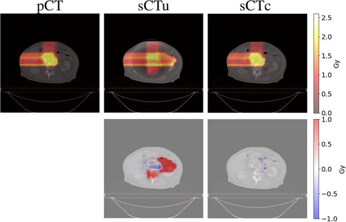
Figure 8. Example of DVH computed for ROI and two organs at risk (bowel and stomach). Solid line: pCT, dashed line: sCTu, dotted line: sCTc. Synthetic CT scans in this figure were produced using a simulated CBCT as the input.

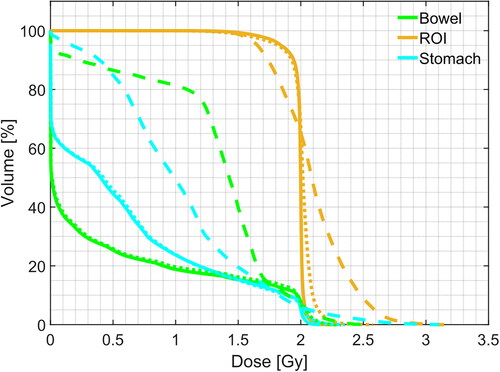
Table 1. Gamma pass rate results for different criteria computed using only the simulated CBCT dataset as input to the framework. Statistical difference in gamma score distributions, between uncorrected and corrected sCT, was found (p < 0.001).

Gamma Criterion	sCTu	sCTc
1%/1 mm	44.68 (6.91)	74.37 (4.63)
2%/2 mm	51.72 (8.15)	87.30 (6.32)
3%/2 mm	53.78 (8.53)	90.26 (5.70)
3%/3 mm	57.57 (7.49)	92.82 (5.94)

DPR at 1% was also found to be significantly higher for the processed sCT than the unprocessed ones (93.97% vs. 79.76%), indicating a 14.21% improvement in dose accuracy with the use of sCTc. In regard to mean dose distribution across the overall dataset, the advantage of sCTc was evident with respect to the overdosing of the sCTu in the ROI (Table 2). The relative percentage error decreased from 6% for sCTu up to 2% for sCTc. A greater advantage was achieved in terms of unwanted doses distributed at the bowel as 97% against 2%, with respect to the nominal toxicity in the pCT. Likewise, the relative toxicity in the stomach decreased from 49% up the 2%. For D5, the correction was effective in reducing the overexposure found in the unprocessed sCT. For D95, the correction underestimated the dose of about 5%. As far as OAR is concerned, the correction was again effective in ensuring a low dose, very similar to that one obtained in the planning CT, at both bowel and stomach. Interestingly, the IQR range of 0.12 Gy (D95) for the stomach potentially delivered when using the sCTu was completely zeroed by the correction.

Table 2. Mean doses, D5, and D95, measured on ROI, bowel, and stomach, computed using only the simulated CBCT dataset as input to the framework. Values are expressed as median(IQR) Gy.

		Mean dose	D5	D95
	pCT	1.98 (0.01)	2.04 (0.01)	1.86 (0.07)
ROI	sCTu	2.10 (0.09)	2.61 (0.28)	1.64 (0.10)
	sCTc	1.93 (0.08)	2.09 (0.05)	1.54 (0.28)
	pCT	0.47 (0.44)	2.01 (0.04)	0.00 (0.00)
Bowel	sCTu	0.93 (0.52)	2.06 (0.31)	0.00 (0.00)
	sCTc	0.48 (0.40)	2.00 (0.13)	0.00 (0.00)
	pCT	0.65 (0.27)	2.01 (0.03)	0.00 (0.00)
Stomach	sCTu	0.97 (0.35)	2.14 (0.24)	0.00 (0.12)
	sCTc	0.64 (0.29)	2.02 (0.11)	0.00 (0.00)

3.4. Treatment planning evaluation – real data

Each result presented in previous sections referred to simulated CBCT. The following results refer to sCT generated using real CBCT as the input data in order to show the quality of the treatment planning with real-world data. As explained in Section 2.2.4, a rigid registration step was added to the pipeline just before the pCT override (Figure 9). Once again, the comparison of the treatment plans generated for each method confirmed an improved similarity between sCTc and pCT with respect to their uncorrected equivalent. Figure 10) depicts an example case in which it is possible to observe again how the beam path exceeded the ROI with a consequent overdosing in the adjacent healthy tissues when computed on sCTu. However, the sCTc treatment plan effectively reduced the overdosing and corrected this pattern, leading to a beam path that closely resembled the pCT plan and reducing the differences (cfr. Figure 10 bottom row). The corresponding dose-volume histogram for the test subject (Figure 11) further supported this observation. Looking at the ROI lines, the sCTc (orange dotted line) followed the profile of pCT (orange solid line) more closely than the sCTu (orange dashed line). Even if the corrected plan slightly overdosed about 60% of the volume, the effect is reduced compared to the uncorrected plan, which presented a smoother slope for the entirety of the ROI, giving 1.25 Gy to the 100% of the volume instead of the 2 Gy of the prescribed dose and overdosing the rest. This observation became even more apparent when considering the organs at risk (represented by the green and light blue lines). Specifically, the corrected treatment plan for the bowel closely replicated the prescribed one, demonstrating a good level of accuracy.

Figure 9. Overlay of corrected CBCT (pink) on pCT (green) before (left) and after (right) rigid registration. It can be seen that the registration was effective in the alignment of the bony structures. Each image is displayed with Window = 1300, Level = 0.

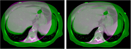
Figure 10. Example of dose planning for an axial slice of a subject for the original pCT, sCTu, and sCTc (upper row). The difference between both sCT treatment plans with respect to the original pCT plan is shown in the bottom row. Synthetic CT scans in this figure were produced using a real CBCT as the input.

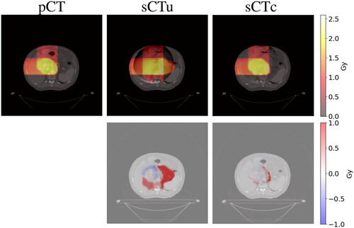
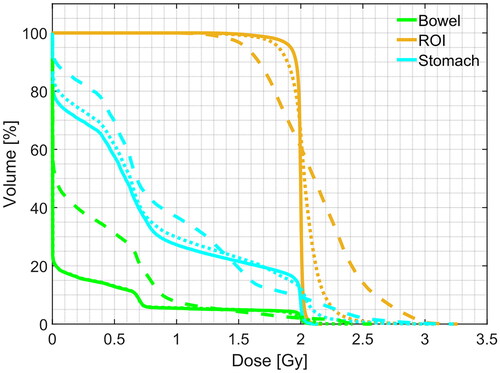
Figure 11. Example of DVH computed for ROI and two organs at risk (bowel and stomach). Solid line: pCT, dashed line: sCTu, dotted line: sCTc. Synthetic CT scans in this figure were produced using a real CBCT as the input.

For a quantitative comparison, the GPR results computed on the entire dataset are summarized in Table 3 as median (IQR). Again, even in the presence of real CBCT overridden to the pCT, the median gamma pass rates for all the computed criteria were consistently higher for the sCTc, with the most significant improvement observed for the 3%/2 mm criterion (23% difference).

Table 3. Gamma pass rate results for different criteria computed using real CBCT dataset as input to the framework. Statistical difference in gamma score distributions, between uncorrected and corrected sCT, was found (p < 0.001).

Gamma Criterion	sCTu	sCTc
1%/1 mm	49.73 (14.84)	71.97 (7.01)
2%/2 mm	61.41 (14.17)	84.37 (5.89)
3%/2 mm	65.36 (14.17)	87.20 (5.79)
3%/3 mm	70.11 (13.66)	89.87 (5.26)

Regarding the average dose distribution, the superiority of sCTc over sCTu in terms of overdosing within the ROI was evident, as indicated in Table 4. The relative percentage error decreased from 3% for sCTu to 1% for sCTc. Furthermore, a significant advantage was also achieved in terms of undesired doses in the bowel, with error percentages of 31% (sCTu) and 13% (sCTc) in comparison to the nominal toxicity in the pCT. Similarly, the relative toxicity in the stomach decreased from 12% to 3%.

Table 4. Mean doses, D5, and D95, measured on ROI, bowel, and stomach, computed using only the real CBCT dataset as input to the framework. Values are expressed as median(IQR) Gy.

		Mean dose	D5	D95
	pCT	1.98 (0.01)	2.04 (0.01)	1.86 (0.07)
ROI	sCTu	2.03 (0.08)	2.37 (0.21)	1.73 (0.13)
	sCTc	1.96 (0.06)	2.11 (0.07)	1.69 (0.18)
	pCT	0.47 (0.44)	2.01 (0.04)	0.00 (0.00)
Bowel	sCTu	0.62 (0.43)	2.05 (0.22)	0.00 (0.00)
	sCTc	0.41 (0.29)	2.00 (0.12)	0.00 (0.00)
	pCT	0.65 (0.27)	2.01 (0.03)	0.00 (0.00)
Stomach	sCTu	0.73 (0.31)	2.12 (0.15)	0.00 (0.00)
	sCTc	0.63 (0.26)	2.02 (0.06)	0.00 (0.00)

4. Discussion

This work proposed a novel image-processing framework for generating synthetic CT scans, which combines the original planning CT with routine CBCT scans, usable to update the dosimetry plan in proton therapy. The core of the framework was represented by a deep learning model, namely a cycle-consistency GAN, to correct the scatter artifacts in the CBCT images and calibrate intensity values, in the proper HU range. Especially, the framework was shown to properly address CBCT equipment scanning narrow FOV [44]. To the aim, the public dataset of patient-paired CT-CBCT scans, named Pancreatic-CT-CBCT-SEG [32], was exploited because of clinically consistent segmentation of ROI and OAR across all the considered patients. From the CT scans, physically consistent simulated CBCT were generated by means of the Monte Carlo algorithm, also accounting for narrow FOV. Especially, Monte Carlo parameter tuning was set according to the CBCT equipment and the acquisition setup at the CNAO. The cGAN-based correction mapped synthetic uncorrected CT into synthetic corrected CT. We remark that, as long as the dataset used to train the network is representative of the data expected to be used in clinical practice, the methodology remains robust. In terms of robustness, the applied methodology did not require retraining the model when moving from simulated to real data. Generally speaking, as soon as the predicted data are no longer satisfactory, the model can be retrained with data taken from the actual clinical setup.

The available segmentations granted replicating the particle beam planning, computed on the original CT, to the corrected sCT for straightforward comparison. The obtained results confirmed, both qualitatively and quantitatively, the capability of the cGAN-based to correct CBCT into CT-compatible images. As shown, the intensity profiles were rectified adequately thanks to the reduction of cupping and truncation artifacts (cfr. Figure 5). A significant increase in PSNR, SSIM, and MAE metrics testified to the effectiveness of the methodology (cfr. Figure 6). Dosimetry computed on uncorrected sCT featured overdosing, especially at OAR (cfr. Tables 1 and 2). An inaccurate assessment of tissue densities was made due to the lack of HU calibration. The proton dosimetry computation is strongly affected by the gradient between CBCT and pCT if HU correction is not properly performed, as the result obtained on sCTu confirmed. The difference in grayscale values between the original CBCT and pCT caused a discontinuity in the volume (cfr. Figure 5), leading to errors in particle beam path computation. Conversely, the dosimetric plan computed on the corrected sCT confirmed the consistency of the plan computed on the corresponding CT scan (cfr. Table 1). The proposed method showed promising preliminary results in terms of proton dosimetry consistency. The American Association of Physicists in Medicine (AAPM) Task Group 218 defined acceptance criteria for tolerance and action limits as exceeding 95% and falling below 90%, respectively, for a 3%/2 mm GPR standard [49]. While not completely in agreement with the upper threshold, the 90.26% found in this work (cfr. Table 1) is to be deemed reasonable. Nonetheless, such value, overcoming the lower 90% action limit threshold, makes the methodology promising for clinical application. In order to avoid confounding factors induced by organ deformation, this work used simulated CBCT by means of the Monte Carlo approach, so that differences between the images were exclusively due to artifacts rather than anatomy. This allowed us to use the same lesion and OAR segmentation used to compute the reference treatment plan. However, results obtained using real-world CBCT as input to the framework confirmed the feasibility of the approach (cfr. Table 3). Real data resulted in generally lower performances when compared to the simulated ones. This was mainly due to the anatomical changes when in the presence of volume acquired on different days during the treatment. It is important to remember that the pelvic site, the subject of this study, contains soft tissue that implies relative movement between organs and the generation of air bubbles [15,50]. Moreover, during the treatment, the patient often loses weight, and the tumor changes shape due to the treatment itself. The CBCT volumes were overridden on the corresponding pCT without any other image fusion techniques. We are aware that this approach is not always viable, especially when the pCT is distant from CBCT acquisition in terms of time. However, many centers are already adopting some immobilization techniques (e.g. custom thermoplastic masks) for patient immobilization on the treatment couch. This helps minimize relative movements between acquisitions. Additionally, a 3D-3D rigid registration step, primarily guided by bony structures between CBCT and pCT, was performed to minimize differences between the two volumes before overriding. When the gradient between the two volumes is considered excessive, it is still advisable to acquire a revaluation CT following the traditional protocol.

Comparison with works in the literature using deep learning to correct CBCT and test proton dosimetry showcased the consistency of the methodology in terms of GPR 2%/2 mm results, even though slightly smaller values with respect to that reported in some papers (Table 5). Significantly, our results on simulated and real data differed less than expected. Nonetheless, we note that our study applied the correction to small FOV (204 mm diameter for simulated data and 250 mm for real data) while the mentioned works dealt with mainly wider FOV (about 480 mm diameter on average). All the works in this comparison involved large anatomical sites (e.g. pelvis, thorax, and abdomen) and the patient cohort had a similar size. Remarkably, the comparison highlighted the superiority of the generative adversarial networks [20,51] with respect to traditional UNet [13,52].

Table 5. Comparison of dosimetry results with literature outcomes in terms of GPR2%/2 mm in the domain of proton therapy.

Work	Model	Anatomic Site	axial FOV [mm]	Patient cohort	GPR 2%/2 mm
Hansen et al. [52]	Unet	Pelvis	410	30	53%
Landry et al. [13]	Unet	Pelvis	410	42	85%
Thummerer et al. [53]	UNet	Thorax	500	33	90.7%
Kurz et al. [51]	cGAN	Pelvis	550	33	96%
Uh et al. [20]	cGAN	Abdomen/Pelvis	530	50	98.5%
This work – simulated	cGAN	Pelvis	204	40	87.3%
This work – real	cGAN	Pelvis	250	40	84.4%

Concerning the small FOV, it is fundamental to recall that the volume of interest is entirely contained in the CBCT and that the tissues coming from the pCT are only needed to calculate the beam path when the air/tissue interface is not already embedded in the CBCT [28,29]. In addition, this makes it mandatory to update the segmentation mask. In this work, the FOV was particularly reduced to demonstrate the feasibility of the methodology. In general, the proposed framework can be adopted in all cases in which the district of interest is too large to fit into a single acquisition. Furthermore, the proposed method extends the use of CBCT systems currently used for patient positioning without additional hardware. Considering that daily CBCTs are acquired for patient positioning purposes, the present framework can be used in parallel with the current clinical routine. Moreover, the computation time required to produce an sCT starting from a CBCT is in the order of a few minutes on an average computer, making it compatible with clinical routines. However, in this work, we did not use the treatment plan computed using the CBCT scan acquired at dose delivery time as the ground truth, but the one computed on the original pCT. While we acknowledge that this can be regarded as a shortcoming toward generalization, the feasibility of the overall methodology was showcased. In future work, the method will be evaluated in a real offline therapy context at the CNAO facility [31]. Correction of CBCTs obtained day-by-day during treatment will be used to assess the evolution of the dose plan without the need to acquire additional CTs and administer further toxicity to the patient [6,20]. Finally, no additional hardware will be needed to add to the patient positioning setup in order to increase the FOV for dosimetric evaluation.

5. Conclusions

The present study proposed a generative artificial intelligence tool to correct CBCT scans, acquired with narrow FOV systems, enabling the reduction of scatter and the remap pixel intensity in HU. The methodology made feasible treatment planning updates, which brings the use of CBCT images incrementally closer to clinical translation in proton therapy.

Preprint

This work was submitted to a noncommercial preprint server. It is available at the following link: https://www.preprints.org/manuscript/202304.0596/v2

Abbreviations
CBCT	=	cone-beam computed tomography
cGAN	=	cycle-consistent generative adversarial network
CNN	=	convolutional neural network
CT	=	computed tomography
DCBCT	=	discriminator CBCT
DCT	=	discriminator CT
DPR	=	dose difference pass rate
DVH	=	dose–volume histogram
FOV	=	field of view
G CBCT	=	generator CBCT
G CT	=	generator CT
GPR	=	gamma pass rate
IQR	=	interquartile range
MAE	=	mean absolute error
MC	=	Monte Carlo
OAR	=	organ at risk
pCT	=	planning CT
PSNR	=	peak signal-to-noise ratio
ROI	=	region of interest
sCT	=	synthetic CT
sCTc	=	corrected sCT
sCTu	=	uncorrected sCT
SSIM	=	structural similarity index measure

Acknowledgments

The authors would like to thank Fabio Casaccio for his support in data retrieval.

Disclosure statement

No potential conflict of interest was reported by the author(s).

Data availability statement

The data presented in this study are openly available in The Cancer Imaging Archive (TCIA) at 10.7937/TCIA.ESHQ-4D90. These collections are freely available to browse, download, and use for commercial, scientific and educational purposes as outlined in the Creative Commons Attribution 3.0 Unported License.

Additional information

Funding

This work was supported by CNAO Foundation (Pavia, Italy) and by FAIR (Future of Artificial Intelligence Research) funded in the PNRR-PE program by Italian Ministry of University.

References

- Bortfeld T. IMRT: a review and preview. Phys Med Biol. 2006;51(13):1–15. doi:10.1088/0031-9155/51/13/r21.
- Joseph PM, Spital RD. The effects of scatter in x-ray computed tomography. Med Phys. 1982;9(4):464–472. doi:10.1118/1.595111.
- Schulze R, Heil U, Gross D, et al. Artefacts in CBCT: a review. Dentomaxillofac Radiol. 2011;40(5):265–273. doi:10.1259/dmfr/30642039.
- Kurz C, Kamp F, Park Y-K, et al. Investigating deformable image registration and scatter correction for CBCT-based dose calculation in adaptive IMPT. Med Phys. 2016;43(10):5635–5646. doi:10.1118/1.4962933.
- Thing RS, Bernchou U, Mainegra-Hing E, et al. Hounsfield unit recovery in clinical cone beam CT images of the thorax acquired for image guided radiation therapy. Phys Med Biol. 2016;61(15):5781–5802. doi:10.1088/0031-9155/61/15/5781.
- Giacometti V, Hounsell AR, McGarry CK. A review of dose calculation approaches with cone beam CT in photon and proton therapy. Phys Med. 2020;76:243–276. doi:10.1016/j.ejmp.2020.06.017.
- Sun M, Star-Lack JM. Improved scatter correction using adaptive scatter kernel superposition. Phys Med Biol. 2010;55(22):6695–6720. doi:10.1088/0031-9155/55/22/007.
- Sisniega A, Zbijewski W, Badal A, et al. Monte Carlo study of the effects of system geometry and antiscatter grids on cone-beam CT scatter distributions. Med Phys. 2013;40(5):051915. doi:10.1118/1.4801895.
- Stankovic U, Ploeger LS, Herk M, et al. Optimal combination of anti-scatter grids and software correction for CBCT imaging. Med Phys. 2017;44(9):4437–4451. doi:10.1002/mp.12385.
- Rusanov B, Hassan GM, Reynolds M, et al. Deep learning methods for enhancing cone-beam CT image quality toward adaptive radiation therapy: a systematic review. Med Phys. 2022;49(9):6019–6054. doi:10.1002/mp.15840.
- Kida S, Nakamoto T, Nakano M, et al. Cone beam computed tomography image quality improvement using a deep convolutional neural network. Cureus. 2018;10(4):e2548. doi:10.7759/cureus.2548.
- Jiang Y, Yang C, Yang P, et al. Scatter correction of cone-beam CT using a deep residual convolution neural network (DRCNN). Phys Med Biol. 2019;64(14):145003. doi:10.1088/1361-6560/ab23a6.
- Landry G, Hansen D, Kamp F, et al. Comparing unet training with three different datasets to correct CBCT images for prostate radiotherapy dose calculations. Phys Med Biol. 2019;64(3):035011. doi:10.1088/1361-6560/aaf496.
- Chen L, Liang X, Shen C, et al. Synthetic CT generation from CBCT images via deep learning. Med Phys. 2020;47(3):1115–1125. doi:10.1002/mp.13978.
- Rossi M, Belotti G, Paganelli C, et al. Image-based shading correction for narrow-fov truncated pelvic cbct with deep convolutional neural networks and transfer learning. Med Phys. 2021;48(11):7112–7126. doi:10.1002/mp.15282.
- Kida S, Kaji S, Nawa K, et al. Visual enhancement of cone-beam CT by use of CycleGAN. Med Phys. 2020;47(3):998–1010. doi:10.1002/mp.13963.
- Eckl M, Hoppen L, Sarria GR, et al. Evaluation of a cycle-generative adversarial network-based cone-beam CT to synthetic CT conversion algorithm for adaptive radiation therapy. Phys Med. 2020;80:308–316. doi:10.1016/j.ejmp.2020.11.007.
- Dong G, Zhang C, Liang X, et al. A deep unsupervised learning model for artifact correction of pelvis cone-beam CT. Front Oncol. 2021;11:686875. doi:10.3389/fonc.2021.686875.
- Sun H, Fan R, Li C, et al. Imaging study of pseudo-CT synthesized from cone-beam CT based on 3d CycleGAN in radiotherapy. Front Oncol. 2021;11:603844. doi:10.3389/fonc.2021.603844.
- Uh J, Wang C, Acharya S, et al. Training a deep neural network coping with diversities in abdominal and pelvic images of children and young adults for CBCT-based adaptive proton therapy. Radiother Oncol. 2021;160:250–258. doi:10.1016/j.radonc.2021.05.006.
- Zhao J, Chen Z, Wang J, et al. MV CBCT-based synthetic CT generation using a deep learning method for rectal cancer adaptive radiotherapy. Front Oncol. 2021;11:655325. doi:10.3389/fonc.2021.655325.
- Xie S, Liang Y, Yang T, et al. Contextual loss based artifact removal method on CBCT image. J Appl Clin Med Phys. 2020;21(12):166–177. doi:10.1002/acm2.13084.
- Wu W, Qu J, Cai J, et al. Multiresolution residual deep neural network for improving pelvic CBCT image quality. Med Phys. 2022;49(3):1522–1534. doi:10.1002/mp.15460.
- Rossi M, Cerveri P. Comparison of supervised and unsupervised approaches for the generation of synthetic ct from cone-beam CT. Diagnostics (Basel). 2021;11(8):1435. doi:10.3390/diagnostics11081435.
- Zhang Y, Yue N, Su M-Y, et al. Improving CBCT quality to CT level using deep learning with generative adversarial network. Med Phys. 2021;48(6):2816–2826. doi:10.1002/mp.14624.
- Landry G, Hua C-h Current state and future applications of radiological image guidance for particle therapy. Med Phys. 2018;45(11):e1086–e1095. doi:10.1002/mp.12744.
- Lu W, Yan H, Zhou L, et al. TU-g-141-05: limited field-of-view cone-beam CT reconstruction for adaptive radiotherapy. Med Phys. 2013;40(6Part27):457–457. doi:10.1118/1.4815465.
- Yu VY, Keyrilainen J, Suilamo S, et al. A multi-institutional analysis of a general pelvis continuous hounsfield unit synthetic ct software for radiotherapy. J Appl Clin Med Phys. 2021;22(3):207–215. doi:10.1002/acm2.13205.
- Velten C, Goddard L, Jeong K, et al. Clinical assessment of a novel ring gantry linear accelerator-mounted helical fan-beam kvct system. Adv Radiat Oncol. 2022;7(2):100862. doi:10.1016/j.adro.2021.100862.
- Clackdoyle R, Defrise M. Tomographic reconstruction in the 21st century. IEEE Signal Process Mag. 2010;27(4):60–80. doi:10.1109/MSP.2010.936743.
- Fattori G, Riboldi M, Pella A, et al. Image guided particle therapy in CNAO room 2: implementation and clinical validation. Phys Med. 2015;31(1):9–15. doi:10.1016/j.ejmp.2014.10.075.
- Hong J, Reyngold M, Crane C, et al. Breath-hold CT and cone-beam CT images with expert manual organ-at-risk segmentations from radiation treatments of locally advanced pancreatic cancer (Pancreatic-CT-CBCT-SEG). The Cancer Imaging Archive. 2021. 10.7937/TCIA.ESHQ-4D90
- Poludniowski G, Evans PM, Hansen VN, et al. An efficient monte carlo-based algorithm for scatter correction in keV cone-beam CT. Phys Med Biol. 2009;54(12):3847–3864. doi:10.1088/0031-9155/54/12/016.
- Jan S, Santin G, Strul D, et al. GATE: a simulation toolkit for PET and SPECT. Phys Med Biol. 2004;49(19):4543–4561. doi:10.1088/0031-9155/49/19/007.
- Poludniowski G, Omar A, Bujila R, et al. Technical note: SpekPy v2.0—a software toolkit for modeling x-ray tube spectra. Med Phys. 2021;48(7):3630–3637. doi:10.1002/mp.14945.
- Rit S, Oliva MV, Brousmiche S, et al. The reconstruction toolkit (RTK), an open-source cone-beam CT reconstruction toolkit based on the insight toolkit (ITK). J Phys: Conf Ser. 2014;489:012079. doi:10.1088/1742-6596/489/1/012079.
- Zhu J-Y, Park T, Isola P, et al. Unpaired image-to-image translation using cycle-consistent adversarial networks. In 2017 IEEE International Conference on Computer Vision (ICCV). IEEE, 2017. doi:10.1109/ICCV.2017.244.
- Ulyanov D, Vedaldi A, Lempitsky V. Instance normalization: the missing ingredient for fast stylization. arXiv preprint arXiv:1607.08022. 2016.
- Sharma S, Sharma S, Athaiya A. Activation functions in neural networks. IJEAST. 2020;04(12):310–316. doi:10.33564/IJEAST.2020.v04i12.054.
- Ronneberger O, Fischer P, Brox T. U-Net: convolutional Networks for Biomedical Image Segmentation. arXiv. 2015. doi:10.48550/ARXIV.1505.04597.
- Isola P, Zhu J-Y, Zhou T, et al. Image-to-image translation with conditional adversarial networks. In. 2017 IEEE Conference on Computer Vision and Pattern Recognition (CVPR). IEEE, 2017. doi:10.1109/CVPR.2017.632.
- Chollet F, et al. Keras. https://keras.io. 2015.
- Abadi M, Agarwal A, Barham P, et al. TensorFlow: large-Scale Machine Learning on Heterogeneous Systems. Software available from tensorflow.org, 2015. Available from: http://tensorflow.org/.
- Spadea MF, Maspero M, Zaffino P, et al. Deep learning based synthetic-CT generation in radiotherapy and PET: a review. Med Phys. 2021;48(11):6537–6566. doi:10.1002/mp.15150.
- Horé A, Ziou D. Image quality metrics: PSNR vs. SSIM. In 2010 20th International Conference on Pattern Recognition, pp. 2366–2369, 2010. doi:10.1109/ICPR.2010.579.
- Wang Z, Bovik AC, Sheikh HR, et al. Image quality assessment: from error visibility to structural similarity. IEEE Trans Image Process. 2004;13(4):600–612. doi:10.1109/tip.2003.819861.
- Wieser H-P, Cisternas E, Wahl N, et al. Development of the open-source dose calculation and optimization toolkit matRad. Med Phys. 2017;44(6):2556–2568. doi:10.1002/mp.12251.
- Dreher C, Habermehl D, Ecker S, et al. Optimization of carbon ion and proton treatment plans using the raster-scanning technique for patients with unresectable pancreatic cancer. Radiat Oncol. 2015;10(1). doi:10.1186/s13014-015-0538-x.
- Miften M, Olch A, Mihailidis D, et al. Tolerance limits and methodologies for IMRT measurement-based verification QA: recommendations of AAPM task group no. 218. Med Phys. 2018;45(4):e53–e83. doi:10.1002/mp.12810.
- Niu T, Al-Basheer A, Zhu L. Quantitative cone-beam CT imaging in radiation therapy using planning CT as a prior: first patient studies. Med Phys. 2012;39(4):1991–2000. doi:10.1118/1.3693050.
- Kurz C, Maspero M, Savenije MHF, et al. CBCT correction using a cycle-consistent generative adversarial network and unpaired training to enable photon and proton dose calculation. Phys Med Biol. 2019;64(22):225004. doi:10.1088/1361-6560/ab4d8c.
- Hansen DC, Landry G, Kamp F, et al. ScatterNet: a convolutional neural network for cone-beam CT intensity correction. Med Phys. 2018;45(11):4916–4926. doi:10.1002/mp.13175.
- Thummerer A, Oria CS, Zaffino P, et al. Clinical suitability of deep learning based synthetic CTs for adaptive proton therapy of lung cancer. Med Phys. 2021;48(12):7673–7684. doi:10.1002/mp.15333.