Mathematical analysis of the role of host-to-host transmission of Maize Streak Virus Disease with Atangana-Baleanu derivative

Abstract

In this article a deterministic model for Maize Streak Virus Disease (MSVD) using a fractional-order differential equation with the Atangana-Baleanu Caputo-type operator is developed. Focusing on the role of host-to-host transmission, the it is shown that the presence and stability of equilibria depends on maize field carrying capacity and half-saturation constant of susceptible maize. The MSVD-free equilibrium is globally asymptotically stable when the basic reproduction number is below unity. Local stability conditions for endemic equilibria are established using Lyapunov second technique and Routh-Hurwitz criteria. Matrix-based formulae are also presented for determining bifurcation and it is shown that the model exhibits forward bifurcation. Sensitivity analysis reveals the significant impact of the probability of infection between hosts on MSVD spread. A two-point Lagrange interpolation polynomial is developed for numerical solutions of the model, enabling exploration of theoretical findings and assessment of how epidemiological factors influence MSVD propagation. The paper contributes a comprehensive understanding of the disease's behavior under various conditions.

Keywords:

• Epidemiology
• Maize Streak Virus Disease
• leafhopper
• basic reproduction number

1. Introduction

As the world’s population continues to grow, there is the need to increase food (especially of plant-based foods) production, since a greater portion of the food consumed worldwide is from plants. With climate change, increased human travel and increased human encroachment of forests, comes a myriad of diseases that hitherto were uncommon in humans, plants and animals. Maize has been estimated to be the second most valuable food crop (Food and Agriculture Organization [FAO], 2016). While there has been a consistent global increase in maize production since the late 1990s, the growth in maize production in Africa has not been as much as in other continents. For instance, while the annual maize production in the United States increased from 3.92 tons in 1961 to 11.86 tons in 2018, the African continent’s maize production only increased from 1.04 tons to 2.04 tons within the same period (Ritchie & Roser, 2013). This is largely due to improved commercialization of farming in the advanced countries unlike the subsistence farming system that is used in most parts of Africa. A significant proportion of global annual crop loss has been attributed to pests and diseases (FAO, 2021). Among the various diseases and pests affecting maize plants, the third most severe is Maize Streak Virus Disease (MSVD). This particular disease holds the highest prevalence among all maize-related illnesses in sub-Saharan Africa, as documented by (Pratt & Gordon, 2010). As the world strives towards achieving zero hunger by 2030, efforts at increasing food production continue to be essential and hence, the need for novel strategies of reducing or eliminating plant diseases and pest are very important.

Mathematical modelling continues to play an indispensable role in improving our understanding of the spread and control of infectious diseases in humans (Ain et al., 2022; Seidu, 2020; Seidu & Makinde, 2014), animals (Baloba, Seidu, & Bornaa, 2020) and plants (Alemneh, Kassa, & Godana, 2021; Alemneh, Makinde, & Theuri, 2020; Aloyce & Kuznetsov, 2017; Ayembillah, Seidu, & Bornaa, 2022; Seidu, Asamoah, Wiah, & Ackora-Prah, 2022; van Maanen & Xu, 2003). The MSVD has received its fair share of attention from Mathematical modelling (Alemneh et al., 2020, 2021; Aloyce & Kuznetsov, 2017; Seidu et al., 2022). Specifically, the authors in (Aloyce & Kuznetsov, 2017) explored Maize Lethal Necrosis Disease (MLND) dynamics and observed that, targeting disease transmission rates could be useful in curbing the spread of MLND. In Collins and Duffy (2016), an optimal control model was structured to identify the most economically efficient approach for mitigating foliar diseases in maize. The findings indicated that implementing disease-resistant maize seeds, promptly removing infected plants, and initiating pesticide use at the disease’s onset can effectively decrease the propagation of foliar diseases. An ecoepidemiological model was proposed in Alemneh, Makinde, & Mwangi Theuri (2019) using Hollings type II functional response form for vector-to-host transmission to describe the dynamics of MSVD. It was observed that the spread of MSVD largely depends on transmission rates and the rate at which leafhoppers prey on susceptible maize plants. Following from the findings of Alemneh et al. (2019), an optimal control problem was proposed in Alemneh et al. (2020) in order to determine the effect of various control strategies on the control of MSVD. In a recent study by Seidu et al. (2022), an optimal control problem was introduced to assess the economic viability of different approaches in containing the spread of MSVD. The study demonstrated that the strategy with the best cost-effectiveness entails the concurrent execution of four controls: regulating transmission, managing predation on maize plants, eliminating infected plants, and employing insecticides. Another interesting work on mathematical modelling of MSVD can be found in Ayembillah et al. (2022). It is noteworthy to state that, to the best of our knowledge, in most of the models constructed to describe the dynamics of MSVD, the role of transmission from infected host tissue to susceptible host tissue has not been considered. Fractional-order models have been shown to be more appropriate than their integer-order counterparts because of their inherent memory effect that makes their predictions better. This is largely because, while solutions of integer-order models rely only on the immediate previous data to determine the current state, solutions of fractional-order models rely on all previous data of the system. This feature of fractional-order models, called the memory property makes them more realistic than their integer-order counterparts. The use of fractional order differential equation models in modelling MSVD is scanty in the literature (Ameen, Baleanu, & Ali, 2022; Kumar, Erturk, Vellappandi, Trinh, & Govindaraj, 2022). The main goal of this paper therefore is to construct and study a MSVD model with Atangana-Baleanu type derivative that incorporates host-to-host transmission in the dynamics of the disease. The Atangana-Baleanu is an extension (Atangana & Baleanu, 2016) of the classical Riemann-Liouville fractional derivative, defined by a parameter, α, which allows for more flexibility in representing fractional order derivatives. The main novelty in this paper is its incorporation of combination of host-to-host transmission of MSVD and fractional-order so that the dynamics of MSVD can be more properly captured. As far as we are aware, this particular combination of methods has not been previously explored in existing literature. Hence, its application serves to enhance the existing body of knowledge in the domain of MSVD modelling.

The next section details the methodical development of the mathematical model of interest. Section 3 provides an overview of some essential qualitative characteristics of the model. The formulation of the numerical scheme employed to solve the proposed FODE model is expounded in Section 4. This scheme is then applied to solve the FODE model for the purpose of carrying out numerical experiments in Section 5. The outcomes of the simulations are discussed in Section 6.

2. The MSVD model

When a swarm of leafhoppers invade a maize field, not only do they consume parts of the maize plants, but they may also infect susceptible plants with the Maize Streak Virus. The spread of MSVD is considered such that leafhopper population of size N_L is compartmentalized into two groups consisting of susceptible leafhopper population of size S_L and infected leafhopper population of size I_L. The infected leafhoppers transmit the Maize Streak Virus to susceptible maize plants of population size S_M. Susceptible maize that get deposits of the virus then join an exposed maize class of size E_M which can then progress into an infected class of population size I_M at rate δ depending on several factors including susceptibility of the maize plant, viral load deposited by the leafhopper among others. Exposure of maize plants occurs due to effective deposition of the virus on the leaves by the infected leafhoppers at rate $\frac{{\beta }_1{I}_L{S}_M}{H_1+S_M}.$ Here, the parameter β₁ represents the probability of infection per effective contact between infected leafhopper and a susceptible maize plant, while H₁ represents the half-saturation constant of predation of susceptible maize plants. Exposure is also assumed to be established when virus in infected maize plants are transported or moved to healthy plant parts at rate $\frac{{\beta }_2{I}_M{S}_M}{H_1+S_M}.$ The parameter β₂ signifies the likelihood of infection per effective interaction between an infected maize plant and a susceptible maize plant. Meanwhile, H₂ denotes the threshold at which susceptibility to infection of susceptible maize plants is halved. Following exposure, it is assumed that maize plants take an average of $1/\delta$ days to become infected, with the rate of transition to the infected class being represented by δ. Susceptible leafhoppers have the potential to contract the virus at a rate of $\frac{{\beta }_3{S}_L{I}_M}{H_2+I_M}$ when they feed on infected plants. Here, β₃ stands for the probability of infection per effective contact between a susceptible leafhopper and an infected maize plant. The natural mortality rates for maize plants and leafhoppers are denoted as μ₁ and μ₂ respectively, while the mortality rate induced by MSVD in plants is given by α. A logistic-type growth pattern is assumed for the susceptible maize population, with an intrinsic growth rate of r, and a constant recruitment of susceptibles into the leafhopper population occurs at a rate of b. The parameter K designates the carrying capacity of the maize field. With these presumptions, the model describing MSV dynamics is represented by the following coupled autonomous equations. (1) $$\begin{array}{c}\frac{\mathrm{d}{S}_M}{\mathrm{d}t}=r{S}_M\left(1-\frac{N_M}{K}\right)-\frac{\left({\beta }_1{I}_L+{\beta }_2{I}_M\right)S_M}{H_1+S_M};\hfill \\ \frac{\mathrm{d}{E}_M}{\mathrm{d}t}=\frac{\left({\beta }_1{I}_L+{\beta }_2{I}_M\right)S_M}{H_1+S_M}-\left(\delta +{\mu }_1\right)E_M;\hfill \\ \frac{\mathrm{d}{I}_M}{\mathrm{d}t}=\delta E_M-(\alpha +{\mu }_1)I_M;\hfill \\ \frac{\mathrm{d}{S}_L}{\mathrm{d}t}=b-\frac{{\beta }_3{I}_M{S}_L}{H_2+I_M}-{\mu }_2{S}_L;\hfill \\ \frac{\mathrm{d}{I}_L}{\mathrm{d}t}=\frac{{\beta }_3{I}_M{S}_L}{H_2+I_M}-{\mu }_2{I}_L.\hfill \end{array}\}$$(1)

Using the Atangan-Baleanu fractional derivative of the Caputo-type, the fractional-order form of (1)(1) $$\begin{array}{c}\frac{\mathrm{d}{S}_M}{\mathrm{d}t}=r{S}_M\left(1-\frac{N_M}{K}\right)-\frac{\left({\beta }_1{I}_L+{\beta }_2{I}_M\right)S_M}{H_1+S_M};\hfill \\ \frac{\mathrm{d}{E}_M}{\mathrm{d}t}=\frac{\left({\beta }_1{I}_L+{\beta }_2{I}_M\right)S_M}{H_1+S_M}-\left(\delta +{\mu }_1\right)E_M;\hfill \\ \frac{\mathrm{d}{I}_M}{\mathrm{d}t}=\delta E_M-(\alpha +{\mu }_1)I_M;\hfill \\ \frac{\mathrm{d}{S}_L}{\mathrm{d}t}=b-\frac{{\beta }_3{I}_M{S}_L}{H_2+I_M}-{\mu }_2{S}_L;\hfill \\ \frac{\mathrm{d}{I}_L}{\mathrm{d}t}=\frac{{\beta }_3{I}_M{S}_L}{H_2+I_M}-{\mu }_2{I}_L.\hfill \end{array}\}$$(1) is given as follows. (2) $$\begin{array}{c}{}_a^{\mathit{\text{ABC}}}{\mathcal{D}}_t^{\varrho }{S}_M(t)=r{S}_M\left(1-\frac{N_M}{K}\right)-\frac{\left({\beta }_1{I}_L+{\beta }_2{I}_M\right)S_M}{H_1+S_M};\hfill \\ {}_a^{\mathit{\text{ABC}}}{\mathcal{D}}_t^{\varrho }{E}_M(t)=\frac{\left({\beta }_1{I}_L+{\beta }_2{I}_M\right)S_M}{H_1+S_M}-\left(\delta +{\mu }_1\right)E_M;\hfill \\ {}_a^{\mathit{\text{ABC}}}{\mathcal{D}}_t^{\varrho }{I}_M(t)=\delta E_M-(\alpha +{\mu }_1)I_M;\hfill \\ {}_a^{\mathit{\text{ABC}}}{\mathcal{D}}_t^{\varrho }{S}_L(t)=b-\frac{{\beta }_3{I}_M{S}_L}{H_2+I_M}-{\mu }_2{S}_L;\hfill \\ {}_a^{\mathit{\text{ABC}}}{\mathcal{D}}_t^{\varrho }{I}_L(t)=\frac{{\beta }_3{I}_M{S}_L}{H_2+I_M}-{\mu }_2{I}_L,\forall t\ge a.\hfill \end{array}\}$$(2)

Here, the order of the fractional derivative is taken as ϱ while the parameter a represents the initial time (we take a = 0 in this work). The total maize plants and leafhoppers are given by $N_M=S_M+E_M+I_M$ and $N_L=S_L+I_L$ respectively. Before the model is analysed, some necessary preliminary definitions on fractional-order calculus are presented as follows:

Definition 2.1.

The Gamma function of n, which generalizes the factorial function is defined as (Kilbas, Srivastava, & Trujillo, 2006) (3) $$\Gamma (n)={\int }_0^{\infty }{t}^{n-1}{e}^{-t}\mathrm{d} t$$(3)

Definition 2.2.

Let f(t) be a continuous function and $\varrho \in (0,1).$ Then the Atangana-Baleanu derivative (Atangana, 2018) is defined as follows (4) $${}_a^{\mathit{\text{ABC}}}{\mathcal{D}}_t^{\varrho }f(t)=\frac{\mathcal{N}(\varrho )}{1-\varrho }{\int }_a^t{f}^{\prime }(\tau )E_{\varrho }\left(-\frac{\varrho {\left(t-\tau \right)}^{\varrho }}{1-\varrho }\right)\mathrm{d}\tau .$$(4) where $\mathcal{N}(\varrho )=1-\varrho +\frac{\varrho }{\Gamma (\varrho )}$ is called the normalization function.

Definition 2.3.

The fractional integral of order $\varrho \in (0,1)$ in the sense of Atangana-Baleanu is defined as follows (Atangana, 2018); (5) $${}_a^{\mathit{\text{ABC}}}{\mathcal{I}}_t^{\varrho }f(t)=\frac{1-\varrho }{\mathcal{N}(\varrho )}f(t)+\frac{\varrho }{\mathcal{N}(\varrho )\Gamma (\varrho )}{\int }_a^{t}f(\tau ){\left(t-\tau \right)}^{\varrho -1}\mathrm{d}\tau$$(5)

All discussions that follow consider the maize and leafhopper populations, as well as the model parameters, to be exclusively non-negative. The subsequent section introduces fundamental qualitative findings regarding the model (1).

3. Qualitative properties of the model

In this section, some basic analytical results are discussed.

Theorem 3.1

(Uniform Boundedness). For all solutions originating from non-negative initial conditions of the model (1)(1) $$\begin{array}{c}\frac{\mathrm{d}{S}_M}{\mathrm{d}t}=r{S}_M\left(1-\frac{N_M}{K}\right)-\frac{\left({\beta }_1{I}_L+{\beta }_2{I}_M\right)S_M}{H_1+S_M};\hfill \\ \frac{\mathrm{d}{E}_M}{\mathrm{d}t}=\frac{\left({\beta }_1{I}_L+{\beta }_2{I}_M\right)S_M}{H_1+S_M}-\left(\delta +{\mu }_1\right)E_M;\hfill \\ \frac{\mathrm{d}{I}_M}{\mathrm{d}t}=\delta E_M-(\alpha +{\mu }_1)I_M;\hfill \\ \frac{\mathrm{d}{S}_L}{\mathrm{d}t}=b-\frac{{\beta }_3{I}_M{S}_L}{H_2+I_M}-{\mu }_2{S}_L;\hfill \\ \frac{\mathrm{d}{I}_L}{\mathrm{d}t}=\frac{{\beta }_3{I}_M{S}_L}{H_2+I_M}-{\mu }_2{I}_L.\hfill \end{array}\}$$(1) , their uniform boundedness is assured within the region Ω, as defined by $$\Omega =\left\{\left(S_M(t),E_M(t),I_M(t),S_L(t),I_M(t)\right)\in {\mathbb{R}}_{+}^5|\underset{t\to \infty }{\mathrm{\text{lim}}}{N}_M(t)\le K,\underset{t\to \infty }{\mathrm{\text{lim}}}{N}_L(t)=\frac{b}{{\mu }_2}\right\}.$$

Proof:

Adding all equations related to maize plants in model (1) gives $$\frac{\mathrm{d}{N}_M}{\mathrm{d}t}=r{S}_M\left(1-\frac{N_M}{K}\right)-{\mu }_1\left(E_M+I_M\right)-\alpha I_M\le r{N}_M\left(1-\frac{N_M}{K}\right)$$

Integrating the inequality above and employing the theory of differential inequalities gives $$0\le N_M(t)\le \frac{\mathit{\text{KN}}(0)}{{\mathrm{e}}^{-\mathit{\text{rt}}}K+\left(1-{\mathrm{e}}^{-\mathit{\text{rt}}}\right)N(0)},$$ so that as $t\to \infty$ we have $0\le N_M(t)\le K.$

Similarly, adding all equations in (1)(1) $$\begin{array}{c}\frac{\mathrm{d}{S}_M}{\mathrm{d}t}=r{S}_M\left(1-\frac{N_M}{K}\right)-\frac{\left({\beta }_1{I}_L+{\beta }_2{I}_M\right)S_M}{H_1+S_M};\hfill \\ \frac{\mathrm{d}{E}_M}{\mathrm{d}t}=\frac{\left({\beta }_1{I}_L+{\beta }_2{I}_M\right)S_M}{H_1+S_M}-\left(\delta +{\mu }_1\right)E_M;\hfill \\ \frac{\mathrm{d}{I}_M}{\mathrm{d}t}=\delta E_M-(\alpha +{\mu }_1)I_M;\hfill \\ \frac{\mathrm{d}{S}_L}{\mathrm{d}t}=b-\frac{{\beta }_3{I}_M{S}_L}{H_2+I_M}-{\mu }_2{S}_L;\hfill \\ \frac{\mathrm{d}{I}_L}{\mathrm{d}t}=\frac{{\beta }_3{I}_M{S}_L}{H_2+I_M}-{\mu }_2{I}_L.\hfill \end{array}\}$$(1) that are related to leafhopper population gives $\frac{\mathrm{d}{N}_L}{\mathrm{d}t}=b-\mu N_L$ whose solution is given by $0\le N_L(t)=\frac{b}{{\mu }_2}+{\mathrm{e}}^{-{\mu }_{2}t}(N_L(0)-\frac{b}{{\mu }_2})$ so that $\underset{t\to \infty }{\mathrm{\text{lim}}}{N}_L(t)=\frac{b}{{\mu }_2}.$ Thus, all solutions of (1)(1) $$\begin{array}{c}\frac{\mathrm{d}{S}_M}{\mathrm{d}t}=r{S}_M\left(1-\frac{N_M}{K}\right)-\frac{\left({\beta }_1{I}_L+{\beta }_2{I}_M\right)S_M}{H_1+S_M};\hfill \\ \frac{\mathrm{d}{E}_M}{\mathrm{d}t}=\frac{\left({\beta }_1{I}_L+{\beta }_2{I}_M\right)S_M}{H_1+S_M}-\left(\delta +{\mu }_1\right)E_M;\hfill \\ \frac{\mathrm{d}{I}_M}{\mathrm{d}t}=\delta E_M-(\alpha +{\mu }_1)I_M;\hfill \\ \frac{\mathrm{d}{S}_L}{\mathrm{d}t}=b-\frac{{\beta }_3{I}_M{S}_L}{H_2+I_M}-{\mu }_2{S}_L;\hfill \\ \frac{\mathrm{d}{I}_L}{\mathrm{d}t}=\frac{{\beta }_3{I}_M{S}_L}{H_2+I_M}-{\mu }_2{I}_L.\hfill \end{array}\}$$(1) initiating from ${\mathbb{R}}_{+}^5\cup \left\{0\right\}$ remain within Ω, concluding the proof. □

Thus, all discussion of the model should be considered to be within this region.

3.1. Existence of equilibria

The MSVD model (1) can be shown to have an MSVD-free fixed point given by ${\mathcal{E}}_0=\left(K,0,0,\frac{b}{{\mu }_2},0\right)$ and possibly some multiple endemic equilibria, which will be discussed later.

The basic reproductive number, denoted as ${\mathcal{R}}_0,$ serves as a metric for estimating the anticipated number of subsequent infections that would arise from the introduction of a single infectious individual into a population entirely susceptible to the disease (Kinene, Luboobi, Nannyonga, & Mwanga, 2015). Through the utilization of the next-generation matrix procedure (Van den Driessche & Watmough, 2008), the basic reproduction number, ${\mathcal{R}}_0,$ is calculated as the spectral radius of the Next-generation matrix. The value of ${\mathcal{R}}_0$ is a pivotal factor for determining the feasibility of disease eradication or its sustained presence (Van den Driessche & Watmough, 2008). The model’s basic reproduction number is obtained as: $${\mathcal{R}}_0={\mathcal{R}}_M+\sqrt{{\mathcal{R}}_{\mathit{\text{ML}}}{\mathcal{R}}_{\mathit{\text{LM}}}+{\mathcal{R}}_M^2},$$ where the reproduction numbers ${\mathcal{R}}_M=\frac{{\beta }_{2}K\delta }{2(H_1+K)(\delta +{\mu }_1)(\alpha +{\mu }_1)},{\mathcal{R}}_{\mathit{\text{LM}}}=\frac{K\delta {\beta }_1}{(\delta +{\mu }_1)(\alpha +{\mu }_1)(H_1+K)}$ and ${\mathcal{R}}_{\mathit{\text{ML}}}=\frac{{\beta }_{3}b}{H_2{\mu }_2{}^2}$ respectively represent the average secondary infections of maize plants through contact with infected maize, the average secondary infections of maize plants through contact with leafhoppers, and the average secondary infections of leafhoppers through contact with infected maize.

Furthermore, the model (Ahmad, Akgül, Khan, Stanimirović, & Chu, 2020) can be shown to have a typical MSVD-persistent fixed point ${\mathcal{E}}^{*}=(S_M^{*},E_M^{*},I_M^{*},S_L^{*},I_L^{*})$ where $$\begin{array}{c}{E}_M^{*}=\frac{b{H}_2\left(\alpha +{\mu }_1\right)\left[\left[\left(H_1+K\right)\left(R_{\mathit{\text{LM}}}{R}_{\mathit{\text{ML}}}+2 R_M\right)-K\right]S_M^{*}-K{H}_1\right]}{\delta \left(H_2{R}_{\mathit{\text{ML}}}{\mu }_2+b\right)\left(\left(K-2 R_M\left(H_1+K\right)\right)S_M^{*}+K{H}_1\right)},\hfill \\ I_M^{*}=\frac{\delta E_M^{*}}{\alpha +{\mu }_1},\hfill \\ S_L^{*}=\frac{b\left(H_2\left(\alpha +{\mu }_1\right)+\delta E_M^{*}\right)}{\left(\delta {\beta }_3+\delta {\mu }_2\right)E_M^{*}+H_2{\mu }_2\left(\alpha +{\mu }_1\right)},\hfill \\ I_L^{*}=\frac{{\beta }_{3}b\delta E_M^{*}}{{\mu }_2\left(\delta \left({\beta }_3+{\mu }_2\right)E_M^{*}+H_2{\mu }_2\left(\alpha +{\mu }_1\right)\right)},\hfill \end{array}\}$$ and $S_M^{*}$ satisfies (6) $${\Psi }_3{\left(S_M^{*}\right)}^3+{\Psi }_2{\left(S_M^{*}\right)}^2+{\Psi }_1{S}_M^{*}+{\Psi }_0=0$$(6) with $$\begin{array}{c}{\Psi }_3=\frac{r}{K}\left(2 {\mathcal{R}}_M\left(H_1+K\right)-K\right);\hfill \\ {\Psi }_2=r\left[\frac{H_{2}b\left(\alpha +{\mu }_1+\delta \right)\left[K-\left(H_1+K\right)\left({\mathcal{R}}_{\mathit{\text{LM}}}{\mathcal{R}}_{\mathit{\text{ML}}}+2 {\mathcal{R}}_M\right)\right]}{K\delta \left({\mu }_2{H}_2{\mathcal{R}}_{\mathit{\text{ML}}}+b\right)}+K-2 {\mathcal{R}}_M\left(H_1+K\right)-H_1\right];\hfill \\ {\Psi }_1=\frac{b{H}_2\left[\left(\alpha +{\mu }_1\right)\left(\delta +{\mu }_1\right)\left(K-\left(H_1+K\right)\left({\mathcal{R}}_{\mathit{\text{LM}}}{\mathcal{R}}_{\mathit{\text{ML}}}+2{\mathcal{R}}_M\right)\right)+r\left(\alpha +{\mu }_1+\delta \right)H_1\right]}{\delta \left({\mu }_2{H}_2{\mathcal{R}}_{\mathit{\text{ML}}}+b\right)}\hfill \\ +\mathit{\text{rK}}{H}_1\text{\hspace{0.17em}and}\hfill \\ {\Psi }_0=\frac{\mathit{\text{bK}}{H}_1{H}_2\left(\delta +{\mu }_1\right)\left(\alpha +{\mu }_1\right)}{\delta \left({\mu }_2{H}_2{\mathcal{R}}_{\mathit{\text{ML}}}+b\right)}.\hfill \end{array}\}$$

 For a given $S_M^{*}>0,$ there exists an epidemiologically reasonable endemic equilibrium if the following condition holds (7) $$S_M^{*}>\frac{K{H}_1}{\left(H_1+K\right)\left[2 {\mathcal{R}}_M\left(1-{\mathcal{R}}_0\right)+{\mathcal{R}}_0{}^2\right]-K}$$(7)

Since, ${\Psi }_0>0,$ the number of endemic equilibria can be completely determined by the signs of, ${\Psi }_1,{\Psi }_2$ and ${\Psi }_3$ as shown in Table 1.

Table 1. Characterization of the number of endemic fixed points of (1)(1) $$\begin{array}{c}\frac{\mathrm{d}{S}_M}{\mathrm{d}t}=r{S}_M\left(1-\frac{N_M}{K}\right)-\frac{\left({\beta }_1{I}_L+{\beta }_2{I}_M\right)S_M}{H_1+S_M};\hfill \\ \frac{\mathrm{d}{E}_M}{\mathrm{d}t}=\frac{\left({\beta }_1{I}_L+{\beta }_2{I}_M\right)S_M}{H_1+S_M}-\left(\delta +{\mu }_1\right)E_M;\hfill \\ \frac{\mathrm{d}{I}_M}{\mathrm{d}t}=\delta E_M-(\alpha +{\mu }_1)I_M;\hfill \\ \frac{\mathrm{d}{S}_L}{\mathrm{d}t}=b-\frac{{\beta }_3{I}_M{S}_L}{H_2+I_M}-{\mu }_2{S}_L;\hfill \\ \frac{\mathrm{d}{I}_L}{\mathrm{d}t}=\frac{{\beta }_3{I}_M{S}_L}{H_2+I_M}-{\mu }_2{I}_L.\hfill \end{array}\}$$(1) .

Signs of coefficients of Equation (6)(6) $${\Psi }_3{\left(S_M^{*}\right)}^3+{\Psi }_2{\left(S_M^{*}\right)}^2+{\Psi }_1{S}_M^{*}+{\Psi }_0=0$$(6)
${\Psi }_3$	${\Psi }_2$	${\Psi }_1$	Number of endemic equilibria
+	+	+	None
−	+	+	1
−	−	+	1
−	−	−	1
+	−	+	2(or none)
+	+	−	2(or none)
+	−	−	2(or none)
−	+	−	3(or 1)

The following results follows from Table 1.

Theorem 3.2.

In addition to the condition in Equation (7)(7) $$S_M^{*}>\frac{K{H}_1}{\left(H_1+K\right)\left[2 {\mathcal{R}}_M\left(1-{\mathcal{R}}_0\right)+{\mathcal{R}}_0{}^2\right]-K}$$(7) , the number of endemic fixed points of (1)(1) $$\begin{array}{c}\frac{\mathrm{d}{S}_M}{\mathrm{d}t}=r{S}_M\left(1-\frac{N_M}{K}\right)-\frac{\left({\beta }_1{I}_L+{\beta }_2{I}_M\right)S_M}{H_1+S_M};\hfill \\ \frac{\mathrm{d}{E}_M}{\mathrm{d}t}=\frac{\left({\beta }_1{I}_L+{\beta }_2{I}_M\right)S_M}{H_1+S_M}-\left(\delta +{\mu }_1\right)E_M;\hfill \\ \frac{\mathrm{d}{I}_M}{\mathrm{d}t}=\delta E_M-(\alpha +{\mu }_1)I_M;\hfill \\ \frac{\mathrm{d}{S}_L}{\mathrm{d}t}=b-\frac{{\beta }_3{I}_M{S}_L}{H_2+I_M}-{\mu }_2{S}_L;\hfill \\ \frac{\mathrm{d}{I}_L}{\mathrm{d}t}=\frac{{\beta }_3{I}_M{S}_L}{H_2+I_M}-{\mu }_2{I}_L.\hfill \end{array}\}$$(1) are characterized as follows.

1. The MSVD model (1)(1) $$\begin{array}{c}\frac{\mathrm{d}{S}_M}{\mathrm{d}t}=r{S}_M\left(1-\frac{N_M}{K}\right)-\frac{\left({\beta }_1{I}_L+{\beta }_2{I}_M\right)S_M}{H_1+S_M};\hfill \\ \frac{\mathrm{d}{E}_M}{\mathrm{d}t}=\frac{\left({\beta }_1{I}_L+{\beta }_2{I}_M\right)S_M}{H_1+S_M}-\left(\delta +{\mu }_1\right)E_M;\hfill \\ \frac{\mathrm{d}{I}_M}{\mathrm{d}t}=\delta E_M-(\alpha +{\mu }_1)I_M;\hfill \\ \frac{\mathrm{d}{S}_L}{\mathrm{d}t}=b-\frac{{\beta }_3{I}_M{S}_L}{H_2+I_M}-{\mu }_2{S}_L;\hfill \\ \frac{\mathrm{d}{I}_L}{\mathrm{d}t}=\frac{{\beta }_3{I}_M{S}_L}{H_2+I_M}-{\mu }_2{I}_L.\hfill \end{array}\}$$(1) has either no equilibrium or two endemic equilibria whenever ${\mathcal{R}}_M>\frac{K}{2(H_1+K)}(\text{ie\hspace{0.5em}}{\Psi }_3>0);$

2. The MSVD model (1)(1) $$\begin{array}{c}\frac{\mathrm{d}{S}_M}{\mathrm{d}t}=r{S}_M\left(1-\frac{N_M}{K}\right)-\frac{\left({\beta }_1{I}_L+{\beta }_2{I}_M\right)S_M}{H_1+S_M};\hfill \\ \frac{\mathrm{d}{E}_M}{\mathrm{d}t}=\frac{\left({\beta }_1{I}_L+{\beta }_2{I}_M\right)S_M}{H_1+S_M}-\left(\delta +{\mu }_1\right)E_M;\hfill \\ \frac{\mathrm{d}{I}_M}{\mathrm{d}t}=\delta E_M-(\alpha +{\mu }_1)I_M;\hfill \\ \frac{\mathrm{d}{S}_L}{\mathrm{d}t}=b-\frac{{\beta }_3{I}_M{S}_L}{H_2+I_M}-{\mu }_2{S}_L;\hfill \\ \frac{\mathrm{d}{I}_L}{\mathrm{d}t}=\frac{{\beta }_3{I}_M{S}_L}{H_2+I_M}-{\mu }_2{I}_L.\hfill \end{array}\}$$(1) has either three endemic equilibria or a unique endemic equilibrium whenever ${\mathcal{R}}_M<\frac{K}{2(H_1+K)}(\text{ie\hspace{0.5em}}{\Psi }_3<0).$

3.2. Local stability of fixed points of (Ahmad et al., 2020)

We examine in this section, the results related to the local asymptotic stability of the fixed points of (1)(1) $$\begin{array}{c}\frac{\mathrm{d}{S}_M}{\mathrm{d}t}=r{S}_M\left(1-\frac{N_M}{K}\right)-\frac{\left({\beta }_1{I}_L+{\beta }_2{I}_M\right)S_M}{H_1+S_M};\hfill \\ \frac{\mathrm{d}{E}_M}{\mathrm{d}t}=\frac{\left({\beta }_1{I}_L+{\beta }_2{I}_M\right)S_M}{H_1+S_M}-\left(\delta +{\mu }_1\right)E_M;\hfill \\ \frac{\mathrm{d}{I}_M}{\mathrm{d}t}=\delta E_M-(\alpha +{\mu }_1)I_M;\hfill \\ \frac{\mathrm{d}{S}_L}{\mathrm{d}t}=b-\frac{{\beta }_3{I}_M{S}_L}{H_2+I_M}-{\mu }_2{S}_L;\hfill \\ \frac{\mathrm{d}{I}_L}{\mathrm{d}t}=\frac{{\beta }_3{I}_M{S}_L}{H_2+I_M}-{\mu }_2{I}_L.\hfill \end{array}\}$$(1) by employing the Lyapunov second method. Additionally, the global stability of the MSVD-free fixed point is investigated utilizing the global stability technique as described in C. Castillo-Chavez, Feng, and Huang (2002).

Theorem 3.3.

The MSVD-free fixed point ${\mathcal{E}}_0$ is locally asymptotically stable whenever ${\mathcal{R}}_0<1.$

Proof:

Evaluating the Jacobian of (1)(1) $$\begin{array}{c}\frac{\mathrm{d}{S}_M}{\mathrm{d}t}=r{S}_M\left(1-\frac{N_M}{K}\right)-\frac{\left({\beta }_1{I}_L+{\beta }_2{I}_M\right)S_M}{H_1+S_M};\hfill \\ \frac{\mathrm{d}{E}_M}{\mathrm{d}t}=\frac{\left({\beta }_1{I}_L+{\beta }_2{I}_M\right)S_M}{H_1+S_M}-\left(\delta +{\mu }_1\right)E_M;\hfill \\ \frac{\mathrm{d}{I}_M}{\mathrm{d}t}=\delta E_M-(\alpha +{\mu }_1)I_M;\hfill \\ \frac{\mathrm{d}{S}_L}{\mathrm{d}t}=b-\frac{{\beta }_3{I}_M{S}_L}{H_2+I_M}-{\mu }_2{S}_L;\hfill \\ \frac{\mathrm{d}{I}_L}{\mathrm{d}t}=\frac{{\beta }_3{I}_M{S}_L}{H_2+I_M}-{\mu }_2{I}_L.\hfill \end{array}\}$$(1) at ${\mathcal{E}}_0$ gives $$\mathcal{J}\left({\mathcal{E}}_0\right)=\left[\begin{array}{ccccc}-r& -r& -r-\frac{{\beta }_{2}K}{H_1+K}& 0& -\frac{{\beta }_{1}K}{H_1+K}\\ 0& -\delta & \frac{{\beta }_{2}K}{H_1+K}& 0& \frac{{\beta }_{1}K}{H_1+K}\\ 0& \delta & -\left(\alpha +{\mu }_1\right)& 0& 0\\ 0& 0& -\frac{b{\beta }_3}{H_2{\mu }_2}& -{\mu }_2& 0\\ 0& 0& \frac{b{\beta }_3}{H_2{\mu }_2}& 0& -{\mu }_2\end{array}\right].$$

 It is easy to observe that two of the eigenvalues of $\mathcal{J}({\mathcal{E}}_0)$ (ie—r and $-{\mu }_2$) are negative while the rest satisfy the following equation. (8) $${\lambda }^3+{\hslash }_2{\lambda }^2+{\hslash }_1\lambda +{\hslash }_0=0,$$(8) where $$\begin{array}{c}{\hslash }_2=\left(\alpha +2{\mu }_1+\delta +{\mu }_2\right),\hfill \\ {\hslash }_1=\left[\left(\delta +{\mu }_1\right)\left(\alpha +{\mu }_1\right)\left(1-2{\mathcal{R}}_M\right)+\left(2 {\mu }_1+\alpha +\delta \right){\mu }_2\right],\hfill \\ {\hslash }_0={\mu }_2\left(\delta +{\mu }_1\right)\left(\alpha +{\mu }_1\right)\left[1-{\mathcal{R}}_{\mathit{\text{ML}}}{\mathcal{R}}_{\mathit{\text{LM}}}-2{\mathcal{R}}_M\right]\hfill \end{array}$$

Employing the Routh-Hurwitz criterion, the real parts of all roots of (8)(8) $${\lambda }^3+{\hslash }_2{\lambda }^2+{\hslash }_1\lambda +{\hslash }_0=0,$$(8) become negative provided that the following conditions are met:

• Condition 1:$1-{\mathcal{R}}_{\mathit{\text{LM}}}{\mathcal{R}}_{\mathit{\text{ML}}}-2{\mathcal{R}}_M>0$ and;

• Condition 2:$$\left[(\delta +{\mu }_1)(\alpha +{\mu }_1)(1-2{\mathcal{R}}_M)+(2 {\mu }_1+\alpha +\delta ){\mu }_2\right]-\frac{(\delta +{\mu }_1)(\alpha +{\mu }_1){\mu }_2(1-{\mathcal{R}}_{\mathit{\text{ML}}}{\mathcal{R}}_{\mathit{\text{LM}}}-2{\mathcal{R}}_M)}{(\alpha +2{\mu }_1+\delta +{\mu }_2)}>0.$$

It is easy to check that whenever ${\mathcal{R}}_0<1,$ then both Conditions are satisfied, concluding the proof. □

Next, in order to analyse the local stability of the endemic fixed points, we adopt the following conventions:

${\xi }_0=1-\frac{E_M^{*}+I_M^{*}+2 S_M^{*}}{K},$ ${\xi }_1=\frac{H_1({\beta }_1{I}_L^{*}+{\beta }_2{I}_M^{*})}{{(H_1+S_M^{*})}^2},$ ${\xi }_2=\frac{S_M^{*}}{H_1+S_M^{*}},$ ${\xi }_3=\frac{S_L^{*}{H}_2}{{(H_2+I_M^{*})}^2}$ and ${\xi }_4=\frac{I_M^{*}}{H_2+I_M^{*}}.$

Evaluating the Jacobian of (1)(1) $$\begin{array}{c}\frac{\mathrm{d}{S}_M}{\mathrm{d}t}=r{S}_M\left(1-\frac{N_M}{K}\right)-\frac{\left({\beta }_1{I}_L+{\beta }_2{I}_M\right)S_M}{H_1+S_M};\hfill \\ \frac{\mathrm{d}{E}_M}{\mathrm{d}t}=\frac{\left({\beta }_1{I}_L+{\beta }_2{I}_M\right)S_M}{H_1+S_M}-\left(\delta +{\mu }_1\right)E_M;\hfill \\ \frac{\mathrm{d}{I}_M}{\mathrm{d}t}=\delta E_M-(\alpha +{\mu }_1)I_M;\hfill \\ \frac{\mathrm{d}{S}_L}{\mathrm{d}t}=b-\frac{{\beta }_3{I}_M{S}_L}{H_2+I_M}-{\mu }_2{S}_L;\hfill \\ \frac{\mathrm{d}{I}_L}{\mathrm{d}t}=\frac{{\beta }_3{I}_M{S}_L}{H_2+I_M}-{\mu }_2{I}_L.\hfill \end{array}\}$$(1) at ${\mathcal{E}}^{*}$ gives $$\mathcal{J}\left({\mathcal{E}}^{*}\right)=\left[\begin{array}{ccccc}{\xi }_1-{\xi }_0& -\frac{r{S}_M}{K}& -\frac{r{S}_M}{K}-{\beta }_2{\xi }_2& 0& -{\beta }_1{\xi }_2\\ {\xi }_1& -\delta -{\mu }_1& {\beta }_2{\xi }_2& 0& {\beta }_1{\xi }_2\\ 0& \delta & -\alpha -{\mu }_1& 0& 0\\ 0& 0& -{\beta }_3{\xi }_3& -{\beta }_3{\xi }_4-{\mu }_2& 0\\ 0& 0& {\beta }_3{\xi }_3& {\beta }_3{\xi }_4& -{\mu }_2\end{array}\right].$$

The Characteristic Polynomial of $\mathcal{J}({\mathcal{E}}^{*})$ can be written as (9) $$\left(\lambda +{\mu }_2\right)\left(K{\lambda }^4+{\mathcal{X}}_3{\lambda }^3+{\mathcal{X}}_2{\lambda }^2+{\mathcal{X}}_1\lambda +{\mathcal{X}}_0\right)=0$$(9) where $$\begin{array}{c}\begin{array}{c}{\mathcal{X}}_3=K\left({\beta }_3{\xi }_4+\alpha +\delta +2 {\mu }_1+{\mu }_2+{\xi }_0-{\xi }_1\right);\hfill \\ {\mathcal{X}}_2=K\left(\alpha +\delta +2 {\mu }_1\right)\left({\beta }_3{\xi }_4+{\mu }_2\right)+K\left({\xi }_0-{\xi }_1\right)\hfill \\ \left({\beta }_3{\xi }_4+\alpha +\delta +2 {\mu }_1+{\mu }_2\right)\hfill \\ \mathrm{\hspace{1em}}\mathrm{\hspace{1em}}+K\left[-\delta {\beta }_2{\xi }_2+\alpha \delta +\alpha {\mu }_1+\delta {\mu }_1+{\mu }_1{}^2\right]+r{S}_M^{*}{\xi }_1;\hfill \\ {\mathcal{X}}_1=[({\xi }_4\left({\xi }_0-{\xi }_1\right)\left(\alpha +\delta +2 {\mu }_1\right)+\left(-\delta {\beta }_2{\xi }_2+\alpha \delta +\alpha {\mu }_1+\delta {\mu }_1+{\mu }_1{}^2\right){\xi }_4-\delta {\beta }_1{\xi }_2{\xi }_3)K+r{S}_M^{*}{\xi }_1{\xi }_4]{\beta }_3\hfill \end{array}\\ \begin{array}{c}\mathrm{\hspace{1em}}\mathrm{\hspace{1em}}+\left({\xi }_0-{\xi }_1\right)\left(\alpha +\delta +2 {\mu }_1\right){\mu }_{2}K+K[\left(-\delta {\beta }_2{\xi }_2+\alpha \delta +\alpha {\mu }_1+\delta {\mu }_1+{\mu }_1{}^2\right)\left({\xi }_0-{\xi }_1+{\mu }_2\right)+\delta {\beta }_2{\xi }_1{\xi }_2]\hfill \\ \mathrm{\hspace{1em}}\mathrm{\hspace{1em}}+\left(\alpha +\delta +{\mu }_1+{\mu }_2\right){\xi }_1{S}_M^{*}r;\hfill \\ {\mathcal{X}}_0=[(\left({\xi }_0-{\xi }_1\right)\left(\left(-\delta {\beta }_2{\xi }_2+\alpha \delta +\alpha {\mu }_1+\delta {\mu }_1+{\mu }_1{}^2\right){\xi }_4-\delta {\beta }_1{\xi }_2{\xi }_3\right)+\delta {\xi }_2\left({\beta }_1{\xi }_3+{\beta }_2{\xi }_4\right){\xi }_1)K\hfill \\ \mathrm{\hspace{1em}}\mathrm{\hspace{1em}}+\left(\alpha +{\mu }_1+\delta \right){\xi }_4{\xi }_1{S}_M^{*}r]{\beta }_3+K{\mu }_2[(-\delta {\beta }_2{\xi }_2+\alpha \delta +\alpha {\mu }_1+\delta {\mu }_1+{\mu }_1{}^2)\left({\xi }_0-{\xi }_1\right)+{\xi }_1\delta {\beta }_2{\xi }_2]\hfill \\ \mathrm{\hspace{1em}}\mathrm{\hspace{1em}}+r{\mu }_2\left(\alpha +{\mu }_1+\delta \right){\xi }_1{S}_M^{*}.\hfill \end{array}\end{array}$$

 Clearly, one of the eigenvalues ($-{\mu }_2$) of $\mathcal{J}({\mathcal{E}}^{*})$ is negative and the following result follows from Routh-Hurwitz stability criterion.

Theorem 3.4.

The MSVD-persistent fixed point ${\mathcal{E}}^{*}$ is locally asymptotically stable whenever the following conditions are satisfied. $${\mathcal{X}}_0>0,{\mathcal{X}}_3>0,{\mathcal{X}}_2-\frac{{\mathcal{X}}_1}{{\mathcal{X}}_3}>0,\text{\hspace{0.5em}and\hspace{0.5em}}{\mathcal{X}}_1-\frac{{\mathcal{X}}_3{\mathcal{X}}_0}{{\mathcal{X}}_2-\frac{{\mathcal{X}}_1}{{\mathcal{X}}_3}}>0.$$

To study the global stability of the MSVD-free fixed point, the technique of C. Castillo-Chavez et al. (2002) is employed. In order to employ this technique, the uninfected sub-system is defined as $$\frac{\mathrm{d}{X}_1}{\mathrm{d}t}=F\left(X_1,X_2\right)$$ where $X_1=(S_M,S_L),$ while the infected subsystem is written as $$\frac{\mathrm{d}{X}_2}{\mathrm{d}t}=G\left(X_1,X_2\right)$$ where $X_2=(E_M,I_M,I_L).$

C. Castillo-Chavez et al. (2002) demonstrated that the disease-free fixed point achieves global stability when the following two conditions are met:

H1: For the reduced sub-system $\mathrm{d}{X}_1/\mathrm{d}t=F(X_1,0),X_1^{*}$ is globally asymptotically stable; and

H2: In the feasible region of the model, $\widehat{G}(X_1,X_2)=A{X}_2-G(X_1,X_2)\ge 0,$ where A, which is the Jacobian of the infected sub-system evaluated at the disease-free equilibrium, is an $M\hspace{0.17em}-$ matrix.

It is easy to show that the reduced sub-system $\mathrm{d}{X}_1/\mathrm{d}t=F(X_1,0)$ has solution $S_M(t)=\frac{K{S}_0}{S_0+{\mathrm{e}}^{-\mathit{\text{rt}}}(K-S_0)}$ and $S_L(t)=\frac{b}{{\mu }_2}-\frac{b}{{\mu }_2}{\mathrm{e}}^{-{\mu }_{2}t}$ which is clearly globally asymptotically stable. Hence, condition H1 is satisfied.

Concerning condition H2, we obtain that $$A=\left[\begin{array}{ccc}-\delta -{\mu }_1& \frac{{\beta }_{2}K}{H_1+K}& \frac{{\beta }_{1}K}{H_1+K}\\ \delta & -\alpha -{\mu }_1& 0\\ 0& \frac{{\beta }_{3}b}{{\mu }_2{H}_2}& -{\mu }_2\end{array}\right]\text{so that}\widehat{G}\left(X_1,X_2\right)=\left(\begin{array}{c}\frac{H_1\left(I_L{\beta }_1+I_M{\beta }_2\right)\left(K-S_M\right)}{\left(H_1+K\right)\left(H_1+S_M\right)}\\ 0\\ \frac{I_M{\beta }_3}{H_2+I_M}\left(\frac{b}{{\mu }_2}-S_L+\frac{b{I}_M}{H_2{\mu }_2}\right)\end{array}\right)$$

Since $N_M\le K$ and $N_L=\frac{b}{{\mu }_2}$ inside the feasible region of the model (1)(1) $$\begin{array}{c}\frac{\mathrm{d}{S}_M}{\mathrm{d}t}=r{S}_M\left(1-\frac{N_M}{K}\right)-\frac{\left({\beta }_1{I}_L+{\beta }_2{I}_M\right)S_M}{H_1+S_M};\hfill \\ \frac{\mathrm{d}{E}_M}{\mathrm{d}t}=\frac{\left({\beta }_1{I}_L+{\beta }_2{I}_M\right)S_M}{H_1+S_M}-\left(\delta +{\mu }_1\right)E_M;\hfill \\ \frac{\mathrm{d}{I}_M}{\mathrm{d}t}=\delta E_M-(\alpha +{\mu }_1)I_M;\hfill \\ \frac{\mathrm{d}{S}_L}{\mathrm{d}t}=b-\frac{{\beta }_3{I}_M{S}_L}{H_2+I_M}-{\mu }_2{S}_L;\hfill \\ \frac{\mathrm{d}{I}_L}{\mathrm{d}t}=\frac{{\beta }_3{I}_M{S}_L}{H_2+I_M}-{\mu }_2{I}_L.\hfill \end{array}\}$$(1) , it is clear that $\widehat{G}(X_1,X_2)\ge 0,$ satisfying condition H2, and Theorem 3.5 is easily established.

Theorem 3.5.

The condition ${\mathcal{R}}_0<1$ guarantees global asymptotic stability of ${\mathcal{E}}_0.$

Theorem 3.5 indicates that it is possible to eradicate MSVD irrespective of initial conditions on the maize field as long as the basic reproduction can be kept below unity.

3.3. Bifurcation analysis

By selecting ${\beta }_1^{*}=\frac{H_2(\delta +{\mu }_1)(\alpha +{\mu }_1)(H_1+K){\mu }_2{}^2}{{\beta }_{3}b\delta K}\left[1-\frac{K{\beta }_2\delta }{(H_1+K)(\delta +{\mu }_1)(\alpha +{\mu }_1)}\right]$ as the bifurcation parameter, it can be shown that the Jacobian matrix of the model (1)(1) $$\begin{array}{c}\frac{\mathrm{d}{S}_M}{\mathrm{d}t}=r{S}_M\left(1-\frac{N_M}{K}\right)-\frac{\left({\beta }_1{I}_L+{\beta }_2{I}_M\right)S_M}{H_1+S_M};\hfill \\ \frac{\mathrm{d}{E}_M}{\mathrm{d}t}=\frac{\left({\beta }_1{I}_L+{\beta }_2{I}_M\right)S_M}{H_1+S_M}-\left(\delta +{\mu }_1\right)E_M;\hfill \\ \frac{\mathrm{d}{I}_M}{\mathrm{d}t}=\delta E_M-(\alpha +{\mu }_1)I_M;\hfill \\ \frac{\mathrm{d}{S}_L}{\mathrm{d}t}=b-\frac{{\beta }_3{I}_M{S}_L}{H_2+I_M}-{\mu }_2{S}_L;\hfill \\ \frac{\mathrm{d}{I}_L}{\mathrm{d}t}=\frac{{\beta }_3{I}_M{S}_L}{H_2+I_M}-{\mu }_2{I}_L.\hfill \end{array}\}$$(1) at ${\mathcal{E}}_0$ possesses a simple eigenvalue. Consequently, the centre manifold theorem (B. Castillo-Chavez & Song, 2004) can be applied to investigate the occurrence and direction of bifurcation within the model. The theorem outlined in B. Castillo-Chavez and Song (2004) asserts that the behaviour of the model can be entirely described by the bifurcation coefficients a and b, which are defined as follows: $$\mathbf{a}=\sum _{i,j,k=1}^n{v}_k{w}_i{w}_j\frac{{\partial }^2{f}_k}{\partial x_i\partial x_j}\left({\mathcal{E}}_0,{\beta }_1^{*}\right),\text{\hspace{0.5em}and\hspace{0.5em}}\mathbf{b}=\sum _{i,k=1}^n{v}_k{w}_i\frac{{\partial }^2{f}_k}{\partial x_i\partial {\beta }_1}\left({\mathcal{E}}_0,{\beta }_1^{*}\right),$$ where f_k is the $k^{\text{th}}$ component of $f(x)={(f_1(x),f_2(x),f_3(x),f_4(x),f_5(x))}^T,x_1=S_M,x_2=E_M,x_3=I_M,x_4=S_L,x_5=I_L$ and v and w are the left and right eigenvalues of $\mathcal{J}({\mathcal{E}}_0,{\beta }_1^{*}).$

It should be noted that $\frac{{\partial }^2{f}_k}{\partial x_i\partial x_j}$ is the ${(i,j)}^{\text{th}}$ component of the Hessian ${\mathbb{H}}^k$ of f_k and $\frac{{\partial }^2{f}_k}{\partial {\beta }_1^{*}\partial x_i}$ is the ${(k,i)}^{\text{th}}$ component of the ${\beta }_1^{*}\hspace{0.17em}-$ differentiated Jacobian, ${\mathbb{J}}^{{\beta }_1^{*}}=\frac{\partial \mathbb{J}}{\partial {\beta }_1^{*}}$ of the model. With this approach of using Hessian and parameter-differentiated Jacobian, the bifurcation coefficients can be found using the following formulae. $$\mathbf{a}=\sum _i\mathbf{\text{tr}}\left(w{w}^T{\mathbb{H}}_i\right)v_i=\mathbf{\text{tr}}\left(w{w}^T\sum _i{v}_i{\mathbb{H}}_i\right) \text{and}\mathbf{b}=v{\mathbb{J}}^{{\beta }_1^{*}}w.$$

The left and right eigenvectors of $\mathcal{J}({\mathcal{E}}_0,{\beta }_1^{*})$ are given by

$v=(0,\frac{\delta v_3}{\delta +{\mu }_1},v_3,0,\frac{{\beta }_{1}K\delta v_3}{(H_1+K)(\delta +{\mu }_1){\mu }_2})$ and $w={(-\frac{\left[({\mu }_1+r+\alpha +\delta ){\mu }_1+(r+\alpha )\delta +\alpha r\right]w_3}{r\delta },\frac{(\alpha +{\mu }_1)w_3}{\delta },w_3,-\frac{{\beta }_{3}b{w}_3}{{\mu }_2{}^2{H}_2},\frac{{\beta }_{3}b{w}_3}{{\mu }_2{}^2{H}_2})}^T$ where $w_3$ and v₃ are chosen to satisfy $w•v=1(\text{ie}.\hspace{0.5em}{\mathrm{w}}_3{\mathrm{v}}_3\text{=}\frac{({\mathrm{H}}_1\text{+K})(\delta +{\mu }_1){\mu }_2{}^3{\mathrm{H}}_2}{\left[{\mathrm{H}}_2(\alpha +\delta \text{+2} {\mu }_1)({\mathrm{H}}_1\text{+K}){\mu }_2{}^3+{\beta }_3\mathrm{b}\delta {\beta }_1\mathrm{K}\right]}).$

The bifurcation coefficients are therefore obtained as $$\mathbf{a}=-2[\frac{H_1\left({\beta }_2{\mu }_2{}^2{H}_2+b{\beta }_1^{*}{\beta }_3\right)\left[\left(r+\alpha +\delta +{\mu }_1\right){\mu }_1+\left(r+\alpha \right)\delta +\alpha r\right]}{r{\mu }_2{}^2{H}_2\left(\delta +{\mu }_1\right){\left(H_1+K\right)}^2}+\frac{\mathit{\text{bK}}\delta {\beta }_1^{*}{\beta }_3\left({\beta }_3+{\mu }_2\right)}{{\mu }_2{}^3{H}_2{}^2\left(H_1+K\right)\left(\delta +{\mu }_1\right)}]v_3{w}_3{}^2$$ $$\text{and\hspace{0.5em}}\mathbf{b}=\frac{\delta K{\beta }_{3}b{w}_3{v}_3}{\left(\delta +{\mu }_1\right)\left(H_1+K\right){\mu }_2{}^2{H}_2}.$$

 Clearly, $\mathbf{a}<0,\mathbf{b}>0$ and hence by the centre manifold theorem (B. Castillo-Chavez & Song, 2004), the model (1)(1) $$\begin{array}{c}\frac{\mathrm{d}{S}_M}{\mathrm{d}t}=r{S}_M\left(1-\frac{N_M}{K}\right)-\frac{\left({\beta }_1{I}_L+{\beta }_2{I}_M\right)S_M}{H_1+S_M};\hfill \\ \frac{\mathrm{d}{E}_M}{\mathrm{d}t}=\frac{\left({\beta }_1{I}_L+{\beta }_2{I}_M\right)S_M}{H_1+S_M}-\left(\delta +{\mu }_1\right)E_M;\hfill \\ \frac{\mathrm{d}{I}_M}{\mathrm{d}t}=\delta E_M-(\alpha +{\mu }_1)I_M;\hfill \\ \frac{\mathrm{d}{S}_L}{\mathrm{d}t}=b-\frac{{\beta }_3{I}_M{S}_L}{H_2+I_M}-{\mu }_2{S}_L;\hfill \\ \frac{\mathrm{d}{I}_L}{\mathrm{d}t}=\frac{{\beta }_3{I}_M{S}_L}{H_2+I_M}-{\mu }_2{I}_L.\hfill \end{array}\}$$(1) exhibits a forward bifurcation at ${\mathcal{R}}_0=1.$ Thus, ${\mathcal{R}}_0$ determines the stability of the equilibria such that whenever ${\mathcal{R}}_0<1$ then ${\mathcal{E}}_0$ is locally asymptotically stable while the endemic equilibrium is either non-existent or unstable. Also, whenever ${\mathcal{R}}_0>1$ then ${\mathcal{E}}_0$ loses its stability to a locally stable endemic equilibrium point.

3.4. Sensitivity analysis

The normalized forward sensitivity indexes of ${\mathcal{R}}_0$ relative to its parameters are given as follows: $$\begin{array}{cc}{{\rm Y}}_{{\mathcal{R}}_0}^{\alpha }=-\frac{\alpha {\mathcal{R}}_0}{2\left(\alpha +{\mu }_1\right)}\hslash ,\hfill & {{\rm Y}}_{{\mathcal{R}}_0}^b=+\frac{\left({\mathcal{R}}_0-2{\mathcal{R}}_M\right)}{2}\hslash ,\hfill \\ {{\rm Y}}_{{\mathcal{R}}_0}^{{\beta }_1}=+\frac{\left({\mathcal{R}}_0-2{\mathcal{R}}_M\right)}{2}\hslash ,\hfill & {{\rm Y}}_{{\mathcal{R}}_0}^{{\beta }_2}=+{\mathcal{R}}_M\hslash ,\hfill \\ {{\rm Y}}_{{\mathcal{R}}_0}^{{\beta }_3}=+\frac{\left({\mathcal{R}}_0-2{\mathcal{R}}_M\right)}{2}\hslash ,\hfill & {{\rm Y}}_{{\mathcal{R}}_0}^{\delta }=+\frac{{\mu }_1{\mathcal{R}}_0}{2\left(\delta +{\mu }_1\right)}\hslash ,\hfill \\ {{\rm Y}}_{{\mathcal{R}}_0}^{H_1}=-\frac{H_1{\mathcal{R}}_0}{2\left(H_1+K\right)}\hslash ,\hfill & {{\rm Y}}_{{\mathcal{R}}_0}^{H_2}=-\frac{\left({\mathcal{R}}_0-2{\mathcal{R}}_M\right)}{2}\hslash \hfill \\ {{\rm Y}}_{{\mathcal{R}}_0}^K=+\frac{H_1{\mathcal{R}}_0}{2\left(H_1+K\right)}\hslash ,\hfill & {{\rm Y}}_{{\mathcal{R}}_0}^{{\mu }_1}=-\frac{{\mu }_1\left(\alpha +\delta +2 {\mu }_1\right){\mathcal{R}}_0}{2\left(\alpha +{\mu }_1\right)\left(\delta +{\mu }_1\right)}\hslash ,\hfill \\ {{\rm Y}}_{{\mathcal{R}}_0}^{{\mu }_2}=-\left({\mathcal{R}}_0-2{\mathcal{R}}_M\right)\hslash ,\hfill & \hslash =\frac{1}{{\mathcal{R}}_0-{\mathcal{R}}_M},\text{\hspace{0.5em}and\hspace{0.5em}}{\mathcal{R}}_0>2{\mathcal{R}}_M.\hfill \end{array}$$

A positive sensitivity index implies that a parameter’s percentage increase (or decrease) leads to a corresponding absolute percentage increase (or decrease) in ${\mathcal{R}}_0.$ On the other hand, a negative sensitivity index indicates that a parameter’s percentage increase (or decrease) results in a corresponding absolute percentage decrease (or increase) in ${\mathcal{R}}_0.$ Thus, increasing(decreasing) b, β₁, β₂, β₃, δ and K leads to increasing(decreasing) ${\mathcal{R}}_0.$ Also, increasing(decreasing) α, H₁, H₂, μ₁ and μ₂ leads to decreasing(increasing) ${\mathcal{R}}_0.$ Since values of ${\mathcal{R}}_0$ below unity are associated with local asymptotic stability of the MSVD-free equilibrium and consequent eradication of MSVD, efforts should be made at reducing b, β₁, β₂, β₃, δ and K while increasing α, H₁, H₂, μ₁ and μ₂. It should be noted however that it is not in the interest of farmers to reduce K or increase μ₁.

4. Development of a numerical scheme for the solution of (Ahmad, Khan, & Cesarano, 2019)

Most mathematical models are generally nonlinear and their close-form solutions are often not feasible or difficult to find. As the non-linearity of the model increases and the order also becomes complex, the difficulty increases. Thus, solving our current model analytically is not feasible. The need to employ numerical solutions is therefore obvious. Several integration techniques have been developed to solve various forms of differential equations (Ahmad et al., 2019, 2020, and reference therein). In this section, the numerical scheme that will be used to solve the MSVD model (2)(2) $$\begin{array}{c}{}_a^{\mathit{\text{ABC}}}{\mathcal{D}}_t^{\varrho }{S}_M(t)=r{S}_M\left(1-\frac{N_M}{K}\right)-\frac{\left({\beta }_1{I}_L+{\beta }_2{I}_M\right)S_M}{H_1+S_M};\hfill \\ {}_a^{\mathit{\text{ABC}}}{\mathcal{D}}_t^{\varrho }{E}_M(t)=\frac{\left({\beta }_1{I}_L+{\beta }_2{I}_M\right)S_M}{H_1+S_M}-\left(\delta +{\mu }_1\right)E_M;\hfill \\ {}_a^{\mathit{\text{ABC}}}{\mathcal{D}}_t^{\varrho }{I}_M(t)=\delta E_M-(\alpha +{\mu }_1)I_M;\hfill \\ {}_a^{\mathit{\text{ABC}}}{\mathcal{D}}_t^{\varrho }{S}_L(t)=b-\frac{{\beta }_3{I}_M{S}_L}{H_2+I_M}-{\mu }_2{S}_L;\hfill \\ {}_a^{\mathit{\text{ABC}}}{\mathcal{D}}_t^{\varrho }{I}_L(t)=\frac{{\beta }_3{I}_M{S}_L}{H_2+I_M}-{\mu }_2{I}_L,\forall t\ge a.\hfill \end{array}\}$$(2) is developed. The Scheme draws on the technique in Toufik and Atangana (2017) to solve Equation (2)(2) $$\begin{array}{c}{}_a^{\mathit{\text{ABC}}}{\mathcal{D}}_t^{\varrho }{S}_M(t)=r{S}_M\left(1-\frac{N_M}{K}\right)-\frac{\left({\beta }_1{I}_L+{\beta }_2{I}_M\right)S_M}{H_1+S_M};\hfill \\ {}_a^{\mathit{\text{ABC}}}{\mathcal{D}}_t^{\varrho }{E}_M(t)=\frac{\left({\beta }_1{I}_L+{\beta }_2{I}_M\right)S_M}{H_1+S_M}-\left(\delta +{\mu }_1\right)E_M;\hfill \\ {}_a^{\mathit{\text{ABC}}}{\mathcal{D}}_t^{\varrho }{I}_M(t)=\delta E_M-(\alpha +{\mu }_1)I_M;\hfill \\ {}_a^{\mathit{\text{ABC}}}{\mathcal{D}}_t^{\varrho }{S}_L(t)=b-\frac{{\beta }_3{I}_M{S}_L}{H_2+I_M}-{\mu }_2{S}_L;\hfill \\ {}_a^{\mathit{\text{ABC}}}{\mathcal{D}}_t^{\varrho }{I}_L(t)=\frac{{\beta }_3{I}_M{S}_L}{H_2+I_M}-{\mu }_2{I}_L,\forall t\ge a.\hfill \end{array}\}$$(2) as follows:

Denote $\mathcal{X}=(S_M,E_M,I_M,S_L,I_L)$ so that the model (2)(2) $$\begin{array}{c}{}_a^{\mathit{\text{ABC}}}{\mathcal{D}}_t^{\varrho }{S}_M(t)=r{S}_M\left(1-\frac{N_M}{K}\right)-\frac{\left({\beta }_1{I}_L+{\beta }_2{I}_M\right)S_M}{H_1+S_M};\hfill \\ {}_a^{\mathit{\text{ABC}}}{\mathcal{D}}_t^{\varrho }{E}_M(t)=\frac{\left({\beta }_1{I}_L+{\beta }_2{I}_M\right)S_M}{H_1+S_M}-\left(\delta +{\mu }_1\right)E_M;\hfill \\ {}_a^{\mathit{\text{ABC}}}{\mathcal{D}}_t^{\varrho }{I}_M(t)=\delta E_M-(\alpha +{\mu }_1)I_M;\hfill \\ {}_a^{\mathit{\text{ABC}}}{\mathcal{D}}_t^{\varrho }{S}_L(t)=b-\frac{{\beta }_3{I}_M{S}_L}{H_2+I_M}-{\mu }_2{S}_L;\hfill \\ {}_a^{\mathit{\text{ABC}}}{\mathcal{D}}_t^{\varrho }{I}_L(t)=\frac{{\beta }_3{I}_M{S}_L}{H_2+I_M}-{\mu }_2{I}_L,\forall t\ge a.\hfill \end{array}\}$$(2) can be written as $${}_a^{\mathit{\text{ABC}}}{\mathcal{D}}_t^{\varrho }\mathcal{X}=\mathcal{G}\left(t,\mathcal{X}\right)$$ where (10) $$\mathcal{G}\left(t,\mathcal{X}\right)=\left(\begin{array}{l}r{S}_M\left(1-\frac{N_M}{K}\right)-\frac{\left({\beta }_1{I}_L+{\beta }_2{I}_M\right)S_M}{H_1+S_M};\\ \frac{\left({\beta }_1{I}_L+{\beta }_2{I}_M\right)S_M}{H_1+S_M}-\left(\delta +{\mu }_1\right)E_M;\\ \delta E_M-(\alpha +{\mu }_1)I_M;\\ b-\frac{{\beta }_3{I}_M{S}_L}{H_2+I_M}-{\mu }_2{S}_L;\\ \frac{{\beta }_3{I}_M{S}_L}{H_2+I_M}-{\mu }_2{I}_L.\end{array}\right)$$(10)

Using the fundamental theorem of fractional calculus, the Fractional-order Differential Equation (FDE) (Ahmad et al., 2019) can be written equivalently as follows. (11) $$\mathcal{X}(t)-\mathcal{X}(0)=\frac{1-\varrho }{\mathcal{N}(\varrho )}\mathcal{G}\left(t,\mathcal{X}\right)+\frac{\varrho }{\mathcal{N}(\varrho )\Gamma (\varrho )}\underset{0}{\overset{t}{\int }}\mathcal{G}\left(\tau ,\mathcal{X}\right){\left(t-\tau \right)}^{\varrho -1}\mathrm{d}\tau .$$(11)

Employing the discretization $t=t_{n+1},n=0,1,2\dots$ converts the above scheme (11)(11) $$\mathcal{X}(t)-\mathcal{X}(0)=\frac{1-\varrho }{\mathcal{N}(\varrho )}\mathcal{G}\left(t,\mathcal{X}\right)+\frac{\varrho }{\mathcal{N}(\varrho )\Gamma (\varrho )}\underset{0}{\overset{t}{\int }}\mathcal{G}\left(\tau ,\mathcal{X}\right){\left(t-\tau \right)}^{\varrho -1}\mathrm{d}\tau .$$(11) into the following equation. (12) $$\mathcal{X}(t_n+1)=\mathcal{X}(0)+\frac{1-\varrho }{\mathcal{N}(\varrho )}\mathcal{G}\left(t_n,\mathcal{X}\right)+\frac{\varrho }{\mathcal{N}(\varrho )\Gamma (\varrho )}\sum _{k=0}^n\underset{t_k}{\overset{t_{k+1}}{\int }}\mathcal{G}\left(\tau ,\mathcal{X}\right){\left(t_{n+1}-\tau \right)}^{\varrho -1}\mathrm{d}\tau .$$(12)

Specifically, the fractional order MSVD model (2)(2) $$\begin{array}{c}{}_a^{\mathit{\text{ABC}}}{\mathcal{D}}_t^{\varrho }{S}_M(t)=r{S}_M\left(1-\frac{N_M}{K}\right)-\frac{\left({\beta }_1{I}_L+{\beta }_2{I}_M\right)S_M}{H_1+S_M};\hfill \\ {}_a^{\mathit{\text{ABC}}}{\mathcal{D}}_t^{\varrho }{E}_M(t)=\frac{\left({\beta }_1{I}_L+{\beta }_2{I}_M\right)S_M}{H_1+S_M}-\left(\delta +{\mu }_1\right)E_M;\hfill \\ {}_a^{\mathit{\text{ABC}}}{\mathcal{D}}_t^{\varrho }{I}_M(t)=\delta E_M-(\alpha +{\mu }_1)I_M;\hfill \\ {}_a^{\mathit{\text{ABC}}}{\mathcal{D}}_t^{\varrho }{S}_L(t)=b-\frac{{\beta }_3{I}_M{S}_L}{H_2+I_M}-{\mu }_2{S}_L;\hfill \\ {}_a^{\mathit{\text{ABC}}}{\mathcal{D}}_t^{\varrho }{I}_L(t)=\frac{{\beta }_3{I}_M{S}_L}{H_2+I_M}-{\mu }_2{I}_L,\forall t\ge a.\hfill \end{array}\}$$(2) can solved iteratively using the following scheme. (13) $$\begin{array}{c}\begin{array}{c}{S}_M(t_n+1)=S_M(0)+\frac{1-\varrho }{\mathcal{N}(\varrho )}\left(r{S}_M\left(1-\frac{N_M}{K}\right)-\frac{\left({\beta }_1{I}_L+{\beta }_2{I}_M\right)S_M}{H_1+S_M}\right)\hfill \\ +\frac{\varrho }{\mathcal{N}(\varrho )\Gamma (\varrho )}\sum _{k=0}^n\underset{t_k}{\overset{t_{k+1}}{\int }}\left(r{S}_M\left(1-\frac{N_M}{K}\right)-\frac{\left({\beta }_1{I}_L+{\beta }_2{I}_M\right)S_M}{H_1+S_M}\right){\left(t_{n+1}-\tau \right)}^{\varrho -1}\mathrm{d}\tau \hfill \\ E_M(t_n+1)=E_M(0)+\frac{1-\varrho }{\mathcal{N}(\varrho )}\left(\frac{\left({\beta }_1{I}_L+{\beta }_2{I}_M\right)S_M}{H_1+S_M}-\left(\delta +{\mu }_1\right)E_M\right)\hfill \\ +\frac{\varrho }{\mathcal{N}(\varrho )\Gamma (\varrho )}\sum _{k=0}^n\underset{t_k}{\overset{t_{k+1}}{\int }}\left(\frac{\left({\beta }_1{I}_L+{\beta }_2{I}_M\right)S_M}{H_1+S_M}-\left(\delta +{\mu }_1\right)E_M\right){\left(t_{n+1}-\tau \right)}^{\varrho -1}\mathrm{d}\tau \hfill \\ I_M(t_n+1)=I_M(0)+\frac{1-\varrho }{\mathcal{N}(\varrho )}\left(\delta E_M-(\alpha +{\mu }_1)I_M\right)\hfill \end{array}\\ \begin{array}{c}+\frac{\varrho }{\mathcal{N}(\varrho )\Gamma (\varrho )}\sum _{k=0}^n\underset{t_k}{\overset{t_{k+1}}{\int }}\left(\delta E_M-(\alpha +{\mu }_1)I_M\right){\left(t_{n+1}-\tau \right)}^{\varrho -1}\mathrm{d}\tau \hfill \\ S_L(t_n+1)=S_L(0)+\frac{1-\varrho }{\mathcal{N}(\varrho )}\left(b-\frac{{\beta }_3{I}_M{S}_L}{H_2+I_M}-{\mu }_2{S}_L\right)\hfill \\ +\frac{\varrho }{\mathcal{N}(\varrho )\Gamma (\varrho )}\sum _{k=0}^n\underset{t_k}{\overset{t_{k+1}}{\int }}\left(b-\frac{{\beta }_3{I}_M{S}_L}{H_2+I_M}-{\mu }_2{S}_L\right){\left(t_{n+1}-\tau \right)}^{\varrho -1}\mathrm{d}\tau \hfill \\ I_L(t_n+1)=I_L(0)+\frac{1-\varrho }{\mathcal{N}(\varrho )}\left(\frac{{\beta }_3{I}_M{S}_L}{H_2+I_M}-{\mu }_2{I}_L\right)\hfill \\ +\frac{\varrho }{\mathcal{N}(\varrho )\Gamma (\varrho )}\sum _{k=0}^n\underset{t_k}{\overset{t_{k+1}}{\int }}\left(\frac{{\beta }_3{I}_M{S}_L}{H_2+I_M}-{\mu }_2{I}_L\right){\left(t_{n+1}-\tau \right)}^{\varrho -1}\mathrm{d}\tau .\hfill \end{array}\end{array}\}$$(13)

 As in Toufik and Atangana (2017), we employ a two-point Lagrange interpolation polynomial to approximate the integral in the numerical scheme in (12)(12) $$\mathcal{X}(t_n+1)=\mathcal{X}(0)+\frac{1-\varrho }{\mathcal{N}(\varrho )}\mathcal{G}\left(t_n,\mathcal{X}\right)+\frac{\varrho }{\mathcal{N}(\varrho )\Gamma (\varrho )}\sum _{k=0}^n\underset{t_k}{\overset{t_{k+1}}{\int }}\mathcal{G}\left(\tau ,\mathcal{X}\right){\left(t_{n+1}-\tau \right)}^{\varrho -1}\mathrm{d}\tau .$$(12) to obtain the following. (14) $$\begin{array}{c}\mathcal{X}(t_n+1)=\mathcal{X}(0)+\frac{1-\varrho }{\mathcal{N}(\varrho )}\mathcal{G}\left(t_n,{\mathcal{X}}_n\right)\hfill \\ \hspace{1em}+\frac{\varrho }{\mathcal{N}(\varrho )\Gamma (\varrho )}\sum _{k=0}^n[\frac{\mathcal{G}\left(t_k,{\mathcal{X}}_k\right)}{h}\underset{t_k}{\overset{t_{k+1}}{\int }}\left(\tau -t_{k-1}\right){\left(t_{n+1}-\tau \right)}^{\varrho -1}\mathrm{d}\tau -\frac{\mathcal{G}\left(t_{k-1},{\mathcal{X}}_{k-1}\right)}{h}\underset{t_k}{\overset{t_{k+1}}{\int }}\left(\tau -t_k\right){\left(t_{n+1}-\tau \right)}^{\varrho -1}\mathrm{d}\tau ].\hfill \end{array}$$(14)

Further simplification of Equation (14)(14) $$\begin{array}{c}\mathcal{X}(t_n+1)=\mathcal{X}(0)+\frac{1-\varrho }{\mathcal{N}(\varrho )}\mathcal{G}\left(t_n,{\mathcal{X}}_n\right)\hfill \\ \hspace{1em}+\frac{\varrho }{\mathcal{N}(\varrho )\Gamma (\varrho )}\sum _{k=0}^n[\frac{\mathcal{G}\left(t_k,{\mathcal{X}}_k\right)}{h}\underset{t_k}{\overset{t_{k+1}}{\int }}\left(\tau -t_{k-1}\right){\left(t_{n+1}-\tau \right)}^{\varrho -1}\mathrm{d}\tau -\frac{\mathcal{G}\left(t_{k-1},{\mathcal{X}}_{k-1}\right)}{h}\underset{t_k}{\overset{t_{k+1}}{\int }}\left(\tau -t_k\right){\left(t_{n+1}-\tau \right)}^{\varrho -1}\mathrm{d}\tau ].\hfill \end{array}$$(14) gives (15) $$\begin{array}{c}\mathcal{X}(t_n+1)=\mathcal{X}(0)+\frac{1-\varrho }{\mathcal{N}(\varrho )}\mathcal{G}\left(t_n,{\mathcal{X}}_n\right)+\frac{\varrho }{h\mathcal{N}(\varrho )\Gamma (\varrho )}\sum _{k=0}^n\left[\mathcal{G}\left(t_k,{\mathcal{X}}_k\right){\mathcal{A}}_{\varrho ,k,1}-\mathcal{G}\left(t_{k-1},{\mathcal{X}}_{k-1}\right){\mathcal{A}}_{\varrho ,k,2}\right].\hfill \end{array}$$(15) where $$\begin{array}{c}{\mathcal{A}}_{\varrho ,k,1}=\underset{t_k}{\overset{t_{k+1}}{\int }}\left(\tau -t_{k-1}\right){\left(t_{n+1}-\tau \right)}^{\varrho -1}\mathrm{d}\tau =h^{\varrho +1}\left(\frac{{\left(n+1-k\right)}^{\varrho }\left(n-k+2+\varrho \right)-{\left(n-k\right)}^{\varrho }\left(n-k+2+2\varrho \right)}{\varrho \left(\varrho +1\right)}\right),\hfill \\ {\mathcal{A}}_{\varrho ,k,2}=\underset{t_k}{\overset{t_{k+1}}{\int }}\left(\tau -t_k\right){\left(t_{n+1}-\tau \right)}^{\varrho -1}\mathrm{d}\tau =h^{\varrho +1}\left(\frac{{\left(n+1-k\right)}^{\varrho +1}-{\left(n-k\right)}^{\varrho }\left(n-k+1+\varrho \right)}{\varrho \left(\varrho +1\right)}\right)\hfill \end{array}$$

Using the scheme in Equation (15)(15) $$\begin{array}{c}\mathcal{X}(t_n+1)=\mathcal{X}(0)+\frac{1-\varrho }{\mathcal{N}(\varrho )}\mathcal{G}\left(t_n,{\mathcal{X}}_n\right)+\frac{\varrho }{h\mathcal{N}(\varrho )\Gamma (\varrho )}\sum _{k=0}^n\left[\mathcal{G}\left(t_k,{\mathcal{X}}_k\right){\mathcal{A}}_{\varrho ,k,1}-\mathcal{G}\left(t_{k-1},{\mathcal{X}}_{k-1}\right){\mathcal{A}}_{\varrho ,k,2}\right].\hfill \end{array}$$(15) , the scheme in Equation (13)(13) $$\begin{array}{c}\begin{array}{c}{S}_M(t_n+1)=S_M(0)+\frac{1-\varrho }{\mathcal{N}(\varrho )}\left(r{S}_M\left(1-\frac{N_M}{K}\right)-\frac{\left({\beta }_1{I}_L+{\beta }_2{I}_M\right)S_M}{H_1+S_M}\right)\hfill \\ +\frac{\varrho }{\mathcal{N}(\varrho )\Gamma (\varrho )}\sum _{k=0}^n\underset{t_k}{\overset{t_{k+1}}{\int }}\left(r{S}_M\left(1-\frac{N_M}{K}\right)-\frac{\left({\beta }_1{I}_L+{\beta }_2{I}_M\right)S_M}{H_1+S_M}\right){\left(t_{n+1}-\tau \right)}^{\varrho -1}\mathrm{d}\tau \hfill \\ E_M(t_n+1)=E_M(0)+\frac{1-\varrho }{\mathcal{N}(\varrho )}\left(\frac{\left({\beta }_1{I}_L+{\beta }_2{I}_M\right)S_M}{H_1+S_M}-\left(\delta +{\mu }_1\right)E_M\right)\hfill \\ +\frac{\varrho }{\mathcal{N}(\varrho )\Gamma (\varrho )}\sum _{k=0}^n\underset{t_k}{\overset{t_{k+1}}{\int }}\left(\frac{\left({\beta }_1{I}_L+{\beta }_2{I}_M\right)S_M}{H_1+S_M}-\left(\delta +{\mu }_1\right)E_M\right){\left(t_{n+1}-\tau \right)}^{\varrho -1}\mathrm{d}\tau \hfill \\ I_M(t_n+1)=I_M(0)+\frac{1-\varrho }{\mathcal{N}(\varrho )}\left(\delta E_M-(\alpha +{\mu }_1)I_M\right)\hfill \end{array}\\ \begin{array}{c}+\frac{\varrho }{\mathcal{N}(\varrho )\Gamma (\varrho )}\sum _{k=0}^n\underset{t_k}{\overset{t_{k+1}}{\int }}\left(\delta E_M-(\alpha +{\mu }_1)I_M\right){\left(t_{n+1}-\tau \right)}^{\varrho -1}\mathrm{d}\tau \hfill \\ S_L(t_n+1)=S_L(0)+\frac{1-\varrho }{\mathcal{N}(\varrho )}\left(b-\frac{{\beta }_3{I}_M{S}_L}{H_2+I_M}-{\mu }_2{S}_L\right)\hfill \\ +\frac{\varrho }{\mathcal{N}(\varrho )\Gamma (\varrho )}\sum _{k=0}^n\underset{t_k}{\overset{t_{k+1}}{\int }}\left(b-\frac{{\beta }_3{I}_M{S}_L}{H_2+I_M}-{\mu }_2{S}_L\right){\left(t_{n+1}-\tau \right)}^{\varrho -1}\mathrm{d}\tau \hfill \\ I_L(t_n+1)=I_L(0)+\frac{1-\varrho }{\mathcal{N}(\varrho )}\left(\frac{{\beta }_3{I}_M{S}_L}{H_2+I_M}-{\mu }_2{I}_L\right)\hfill \\ +\frac{\varrho }{\mathcal{N}(\varrho )\Gamma (\varrho )}\sum _{k=0}^n\underset{t_k}{\overset{t_{k+1}}{\int }}\left(\frac{{\beta }_3{I}_M{S}_L}{H_2+I_M}-{\mu }_2{I}_L\right){\left(t_{n+1}-\tau \right)}^{\varrho -1}\mathrm{d}\tau .\hfill \end{array}\end{array}\}$$(13) is finally written as (16) $$\begin{array}{c}\begin{array}{c}{S}_M(t_n+1)=S_M(0)+\frac{1-\varrho }{\mathcal{N}(\varrho )}\left(r{S}_M\left(1-\frac{N_M}{K}\right)-\frac{\left({\beta }_1{I}_L+{\beta }_2{I}_M\right)S_M}{H_1+S_M}\right)\hfill \\ +\frac{\varrho }{h\mathcal{N}(\varrho )\Gamma (\varrho )}\sum _{k=0}^n\{\left(r{S}_M(t_k)\left(1-\frac{N_M(t_k)}{K}\right)-\frac{\left({\beta }_1{I}_L(t_k)+{\beta }_2{I}_M(t_k)\right)S_M(t_k)}{H_1+S_M(t_k)}\right){\mathcal{A}}_{\varrho ,k,1}\hfill \\ -\left(r{S}_M(t_{k-1})\left(1-\frac{N_M(t_{k-1})}{K}\right)-\frac{\left({\beta }_1{I}_L(t_{k-1})+{\beta }_2{I}_M(t_{k-1})\right)S_M(t_{k-1})}{H_1+S_M(t_{k-1})}\right){\mathcal{A}}_{\varrho ,k,2}\}\hfill \\ E_M(t_n+1)=E_M(0)+\frac{1-\varrho }{\mathcal{N}(\varrho )}\left(\frac{\left({\beta }_1{I}_L\left(t_n\right)+{\beta }_2{I}_M\left(t_n\right)\right)S_M\left(t_n\right)}{H_1+S_M\left(t_n\right)}-\left(\delta +{\mu }_1\right)E_M\left(t_n\right)\right)\hfill \\ +\frac{\varrho }{h\mathcal{N}(\varrho )\Gamma (\varrho )}\sum _{k=0}^n\{\left(\frac{\left({\beta }_1{I}_L\left(t_k\right)+{\beta }_2{I}_M\left(t_k\right)\right)S_M\left(t_k\right)}{H_1+S_M\left(t_k\right)}-\left(\delta +{\mu }_1\right)E_M\left(t_k\right)\right){\mathcal{A}}_{\varrho ,k,1}\hfill \\ -\left(\frac{\left({\beta }_1{I}_L\left(t_{k-1}\right)+{\beta }_2{I}_M\left(t_{k-1}\right)\right)S_M\left(t_{k-1}\right)}{H_1+S_M\left(t_{k-1}\right)}-\left(\delta +{\mu }_1\right)E_M\left(t_{k-1}\right)\right){\mathcal{A}}_{\varrho ,k,2}\}\hfill \end{array}\\ \begin{array}{c}{I}_M(t_n+1)=I_M(0)+\frac{1-\varrho }{\mathcal{N}(\varrho )}\left(\delta E_M(t_n)-(\alpha +{\mu }_1)I_M(t_n)\right)\hfill \\ \mathrm{\hspace{1em}\hspace{1em}\hspace{1em}}\mathrm{\hspace{1em}}+\frac{\varrho }{h\mathcal{N}(\varrho )\Gamma (\varrho )}\sum _{k=0}^n\{\left(\delta E_M(t_k)-(\alpha +{\mu }_1)I_M(t_k)\right){\mathcal{A}}_{\varrho ,k,1}-\left(\delta E_M(t_{k-1})-(\alpha +{\mu }_1)I_M(t_{k-1})\right){\mathcal{A}}_{\varrho ,k,2}\}\hfill \\ S_L(t_n+1)=S_L(0)+\frac{1-\varrho }{\mathcal{N}(\varrho )}\left(b-\frac{{\beta }_3{I}_M{S}_L}{H_2+I_M}-{\mu }_2{S}_L\right)\hfill \\ +\frac{\varrho }{h\mathcal{N}(\varrho )\Gamma (\varrho )}\sum _{k=0}^n\{\left(b-\frac{{\beta }_3{I}_M(t_k)S_L(t_k)}{H_2+I_M(t_k)}-{\mu }_2{S}_L(t_k)\right){\mathcal{A}}_{\varrho ,k,1}\hfill \\ -\left(b-\frac{{\beta }_3{I}_M(t_{k-1})S_L(t_{k-1})}{H_2+I_M(t_{k-1})}-{\mu }_2{S}_L(t_{k-1})\right){\mathcal{A}}_{\varrho ,k,2}\};\hfill \\ \mathcal{X}(t_n+1)=\mathcal{X}(0)+\frac{1-\varrho }{\mathcal{N}(\varrho )}\left(\frac{{\beta }_3{I}_M(t_n)S_L(t_n)}{H_2+I_M(t_n)}-{\mu }_2{I}_L(t_n)\right)\hfill \\ \mathrm{\hspace{1em}\hspace{1em}\hspace{1em}}\mathrm{\hspace{1em}}+\frac{\varrho }{h\mathcal{N}(\varrho )\Gamma (\varrho )}\sum _{k=0}^n\{\left(\frac{{\beta }_3{I}_M(t_k)S_L(t_k)}{H_2+I_M(t_k)}-{\mu }_2{I}_L(t_k)\right){\mathcal{A}}_{\varrho ,k,1}-\left(\frac{{\beta }_3{I}_M(t_{k-1})S_L(t_{k-1})}{H_2+I_M(t_{k-1})}-{\mu }_2{I}_L(t_{k-1})\right){\mathcal{A}}_{\varrho ,k,2}\}\hfill \end{array}\end{array}\}$$(16)

In the next section, the scheme in Equation (16)(16) $$\begin{array}{c}\begin{array}{c}{S}_M(t_n+1)=S_M(0)+\frac{1-\varrho }{\mathcal{N}(\varrho )}\left(r{S}_M\left(1-\frac{N_M}{K}\right)-\frac{\left({\beta }_1{I}_L+{\beta }_2{I}_M\right)S_M}{H_1+S_M}\right)\hfill \\ +\frac{\varrho }{h\mathcal{N}(\varrho )\Gamma (\varrho )}\sum _{k=0}^n\{\left(r{S}_M(t_k)\left(1-\frac{N_M(t_k)}{K}\right)-\frac{\left({\beta }_1{I}_L(t_k)+{\beta }_2{I}_M(t_k)\right)S_M(t_k)}{H_1+S_M(t_k)}\right){\mathcal{A}}_{\varrho ,k,1}\hfill \\ -\left(r{S}_M(t_{k-1})\left(1-\frac{N_M(t_{k-1})}{K}\right)-\frac{\left({\beta }_1{I}_L(t_{k-1})+{\beta }_2{I}_M(t_{k-1})\right)S_M(t_{k-1})}{H_1+S_M(t_{k-1})}\right){\mathcal{A}}_{\varrho ,k,2}\}\hfill \\ E_M(t_n+1)=E_M(0)+\frac{1-\varrho }{\mathcal{N}(\varrho )}\left(\frac{\left({\beta }_1{I}_L\left(t_n\right)+{\beta }_2{I}_M\left(t_n\right)\right)S_M\left(t_n\right)}{H_1+S_M\left(t_n\right)}-\left(\delta +{\mu }_1\right)E_M\left(t_n\right)\right)\hfill \\ +\frac{\varrho }{h\mathcal{N}(\varrho )\Gamma (\varrho )}\sum _{k=0}^n\{\left(\frac{\left({\beta }_1{I}_L\left(t_k\right)+{\beta }_2{I}_M\left(t_k\right)\right)S_M\left(t_k\right)}{H_1+S_M\left(t_k\right)}-\left(\delta +{\mu }_1\right)E_M\left(t_k\right)\right){\mathcal{A}}_{\varrho ,k,1}\hfill \\ -\left(\frac{\left({\beta }_1{I}_L\left(t_{k-1}\right)+{\beta }_2{I}_M\left(t_{k-1}\right)\right)S_M\left(t_{k-1}\right)}{H_1+S_M\left(t_{k-1}\right)}-\left(\delta +{\mu }_1\right)E_M\left(t_{k-1}\right)\right){\mathcal{A}}_{\varrho ,k,2}\}\hfill \end{array}\\ \begin{array}{c}{I}_M(t_n+1)=I_M(0)+\frac{1-\varrho }{\mathcal{N}(\varrho )}\left(\delta E_M(t_n)-(\alpha +{\mu }_1)I_M(t_n)\right)\hfill \\ \mathrm{\hspace{1em}\hspace{1em}\hspace{1em}}\mathrm{\hspace{1em}}+\frac{\varrho }{h\mathcal{N}(\varrho )\Gamma (\varrho )}\sum _{k=0}^n\{\left(\delta E_M(t_k)-(\alpha +{\mu }_1)I_M(t_k)\right){\mathcal{A}}_{\varrho ,k,1}-\left(\delta E_M(t_{k-1})-(\alpha +{\mu }_1)I_M(t_{k-1})\right){\mathcal{A}}_{\varrho ,k,2}\}\hfill \\ S_L(t_n+1)=S_L(0)+\frac{1-\varrho }{\mathcal{N}(\varrho )}\left(b-\frac{{\beta }_3{I}_M{S}_L}{H_2+I_M}-{\mu }_2{S}_L\right)\hfill \\ +\frac{\varrho }{h\mathcal{N}(\varrho )\Gamma (\varrho )}\sum _{k=0}^n\{\left(b-\frac{{\beta }_3{I}_M(t_k)S_L(t_k)}{H_2+I_M(t_k)}-{\mu }_2{S}_L(t_k)\right){\mathcal{A}}_{\varrho ,k,1}\hfill \\ -\left(b-\frac{{\beta }_3{I}_M(t_{k-1})S_L(t_{k-1})}{H_2+I_M(t_{k-1})}-{\mu }_2{S}_L(t_{k-1})\right){\mathcal{A}}_{\varrho ,k,2}\};\hfill \\ \mathcal{X}(t_n+1)=\mathcal{X}(0)+\frac{1-\varrho }{\mathcal{N}(\varrho )}\left(\frac{{\beta }_3{I}_M(t_n)S_L(t_n)}{H_2+I_M(t_n)}-{\mu }_2{I}_L(t_n)\right)\hfill \\ \mathrm{\hspace{1em}\hspace{1em}\hspace{1em}}\mathrm{\hspace{1em}}+\frac{\varrho }{h\mathcal{N}(\varrho )\Gamma (\varrho )}\sum _{k=0}^n\{\left(\frac{{\beta }_3{I}_M(t_k)S_L(t_k)}{H_2+I_M(t_k)}-{\mu }_2{I}_L(t_k)\right){\mathcal{A}}_{\varrho ,k,1}-\left(\frac{{\beta }_3{I}_M(t_{k-1})S_L(t_{k-1})}{H_2+I_M(t_{k-1})}-{\mu }_2{I}_L(t_{k-1})\right){\mathcal{A}}_{\varrho ,k,2}\}\hfill \end{array}\end{array}\}$$(16) will be used to solve the fractional differential equation model (2)(2) $$\begin{array}{c}{}_a^{\mathit{\text{ABC}}}{\mathcal{D}}_t^{\varrho }{S}_M(t)=r{S}_M\left(1-\frac{N_M}{K}\right)-\frac{\left({\beta }_1{I}_L+{\beta }_2{I}_M\right)S_M}{H_1+S_M};\hfill \\ {}_a^{\mathit{\text{ABC}}}{\mathcal{D}}_t^{\varrho }{E}_M(t)=\frac{\left({\beta }_1{I}_L+{\beta }_2{I}_M\right)S_M}{H_1+S_M}-\left(\delta +{\mu }_1\right)E_M;\hfill \\ {}_a^{\mathit{\text{ABC}}}{\mathcal{D}}_t^{\varrho }{I}_M(t)=\delta E_M-(\alpha +{\mu }_1)I_M;\hfill \\ {}_a^{\mathit{\text{ABC}}}{\mathcal{D}}_t^{\varrho }{S}_L(t)=b-\frac{{\beta }_3{I}_M{S}_L}{H_2+I_M}-{\mu }_2{S}_L;\hfill \\ {}_a^{\mathit{\text{ABC}}}{\mathcal{D}}_t^{\varrho }{I}_L(t)=\frac{{\beta }_3{I}_M{S}_L}{H_2+I_M}-{\mu }_2{I}_L,\forall t\ge a.\hfill \end{array}\}$$(2) .

5. Numerical experiments

Within this section, numerical simulations are carried out to visually demonstrate certain analytical findings as well as to observe the influence of specific model parameters on the transmission dynamics of MSVD. For this purpose, the fractional differential equation model (Ahmad et al., 2019) is solved utilizing the numerical scheme presented in Equation (16)(16) $$\begin{array}{c}\begin{array}{c}{S}_M(t_n+1)=S_M(0)+\frac{1-\varrho }{\mathcal{N}(\varrho )}\left(r{S}_M\left(1-\frac{N_M}{K}\right)-\frac{\left({\beta }_1{I}_L+{\beta }_2{I}_M\right)S_M}{H_1+S_M}\right)\hfill \\ +\frac{\varrho }{h\mathcal{N}(\varrho )\Gamma (\varrho )}\sum _{k=0}^n\{\left(r{S}_M(t_k)\left(1-\frac{N_M(t_k)}{K}\right)-\frac{\left({\beta }_1{I}_L(t_k)+{\beta }_2{I}_M(t_k)\right)S_M(t_k)}{H_1+S_M(t_k)}\right){\mathcal{A}}_{\varrho ,k,1}\hfill \\ -\left(r{S}_M(t_{k-1})\left(1-\frac{N_M(t_{k-1})}{K}\right)-\frac{\left({\beta }_1{I}_L(t_{k-1})+{\beta }_2{I}_M(t_{k-1})\right)S_M(t_{k-1})}{H_1+S_M(t_{k-1})}\right){\mathcal{A}}_{\varrho ,k,2}\}\hfill \\ E_M(t_n+1)=E_M(0)+\frac{1-\varrho }{\mathcal{N}(\varrho )}\left(\frac{\left({\beta }_1{I}_L\left(t_n\right)+{\beta }_2{I}_M\left(t_n\right)\right)S_M\left(t_n\right)}{H_1+S_M\left(t_n\right)}-\left(\delta +{\mu }_1\right)E_M\left(t_n\right)\right)\hfill \\ +\frac{\varrho }{h\mathcal{N}(\varrho )\Gamma (\varrho )}\sum _{k=0}^n\{\left(\frac{\left({\beta }_1{I}_L\left(t_k\right)+{\beta }_2{I}_M\left(t_k\right)\right)S_M\left(t_k\right)}{H_1+S_M\left(t_k\right)}-\left(\delta +{\mu }_1\right)E_M\left(t_k\right)\right){\mathcal{A}}_{\varrho ,k,1}\hfill \\ -\left(\frac{\left({\beta }_1{I}_L\left(t_{k-1}\right)+{\beta }_2{I}_M\left(t_{k-1}\right)\right)S_M\left(t_{k-1}\right)}{H_1+S_M\left(t_{k-1}\right)}-\left(\delta +{\mu }_1\right)E_M\left(t_{k-1}\right)\right){\mathcal{A}}_{\varrho ,k,2}\}\hfill \end{array}\\ \begin{array}{c}{I}_M(t_n+1)=I_M(0)+\frac{1-\varrho }{\mathcal{N}(\varrho )}\left(\delta E_M(t_n)-(\alpha +{\mu }_1)I_M(t_n)\right)\hfill \\ \mathrm{\hspace{1em}\hspace{1em}\hspace{1em}}\mathrm{\hspace{1em}}+\frac{\varrho }{h\mathcal{N}(\varrho )\Gamma (\varrho )}\sum _{k=0}^n\{\left(\delta E_M(t_k)-(\alpha +{\mu }_1)I_M(t_k)\right){\mathcal{A}}_{\varrho ,k,1}-\left(\delta E_M(t_{k-1})-(\alpha +{\mu }_1)I_M(t_{k-1})\right){\mathcal{A}}_{\varrho ,k,2}\}\hfill \\ S_L(t_n+1)=S_L(0)+\frac{1-\varrho }{\mathcal{N}(\varrho )}\left(b-\frac{{\beta }_3{I}_M{S}_L}{H_2+I_M}-{\mu }_2{S}_L\right)\hfill \\ +\frac{\varrho }{h\mathcal{N}(\varrho )\Gamma (\varrho )}\sum _{k=0}^n\{\left(b-\frac{{\beta }_3{I}_M(t_k)S_L(t_k)}{H_2+I_M(t_k)}-{\mu }_2{S}_L(t_k)\right){\mathcal{A}}_{\varrho ,k,1}\hfill \\ -\left(b-\frac{{\beta }_3{I}_M(t_{k-1})S_L(t_{k-1})}{H_2+I_M(t_{k-1})}-{\mu }_2{S}_L(t_{k-1})\right){\mathcal{A}}_{\varrho ,k,2}\};\hfill \\ \mathcal{X}(t_n+1)=\mathcal{X}(0)+\frac{1-\varrho }{\mathcal{N}(\varrho )}\left(\frac{{\beta }_3{I}_M(t_n)S_L(t_n)}{H_2+I_M(t_n)}-{\mu }_2{I}_L(t_n)\right)\hfill \\ \mathrm{\hspace{1em}\hspace{1em}\hspace{1em}}\mathrm{\hspace{1em}}+\frac{\varrho }{h\mathcal{N}(\varrho )\Gamma (\varrho )}\sum _{k=0}^n\{\left(\frac{{\beta }_3{I}_M(t_k)S_L(t_k)}{H_2+I_M(t_k)}-{\mu }_2{I}_L(t_k)\right){\mathcal{A}}_{\varrho ,k,1}-\left(\frac{{\beta }_3{I}_M(t_{k-1})S_L(t_{k-1})}{H_2+I_M(t_{k-1})}-{\mu }_2{I}_L(t_{k-1})\right){\mathcal{A}}_{\varrho ,k,2}\}\hfill \end{array}\end{array}\}$$(16) . Unless otherwise indicated, the following parameter values are employed for all simulations: $$\begin{array}{c}\alpha =0.5,\hspace{0.5em}b=0.0333,{\beta }_1=0.45,{\beta }_2=0.045,{\beta }_3=0.04,\delta =0.05, H_1=0.4,\hfill \\ H_2=0.6,K=10000,{\mu }_1=0.0167,{\mu }_2=0.0377,r=0.0005,\text{\hspace{0.5em}order,\hspace{0.5em}}\varrho =0.95;\hfill \end{array}$$

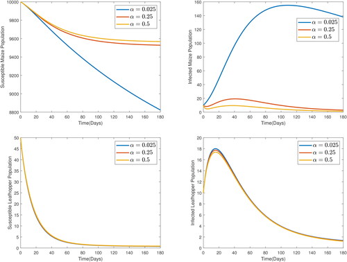
These parameters values were chosen for numerical simulation purposes only. To study the impact of the order of the derivative on the prediction by the model, the model was solved for various values of the order, ϱ. The results are presented in Figure 1, from which, it is observed that the order of the derivative really affects the predictions by the model. Higher orders forecast lower susceptible populations and higher infective populations. Since fractional orders exhibit the memory effect and have been shown to be better, the forecast by the integer order can be considered to have hyped the effect of the MSVD by predicting lower susceptible populations and higher for at least the early stage of the infection. In Figure 2, graphs showing the impact of MSVD-induced death rate in maize are presented. It is observed that, increasing α, the disease-induced death rate in maize plants increases the susceptible maize population while reducing the infected maize population. This is because, as more infectives die, fewer of the susceptibles are exposed to infection. The impact of increases in disease-induced death in maize on susceptible leafhopper population is however not pronounced. A slightly decreased infections in leafhopper populations is observed for increased disease-induced deaths in maize plants.

Figure 1. Impact of the order of the derivative on the prediction of the MSVD model.

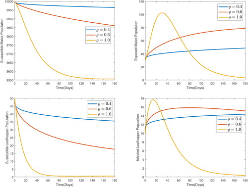
Figure 2. Impact of disease-induced death rate on the dynamics of MSVD.

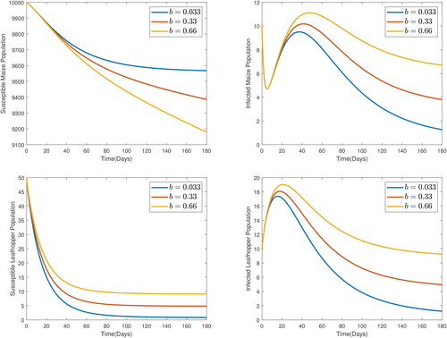
From Figure 3, it is observed that increased leafhopper recruitment leads to increased infections. an increase in b leads to a decrease in the susceptible host population, and an increase in the infected host, susceptible leafhopper and infected leafhopper populations. Thus, inflow of susceptible leafhoppers needs to be curtailed in order to keep the maize field safe.

Figure 3. Impact of leafhopper recruitment on the dynamics of MSVD.

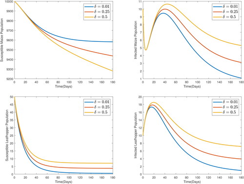
From Figure 4, it is observed that as the rate of progression of exposed maize increases, the number of infected maize increases which leads to more uptake of the virus by the susceptible leafhoppers, all of which lead to a decline in the susceptible maize. Therefore, MSVD-resistant maize needs to be considered to reduce the impact of the disease.

Figure 4. Impact of rate of progression of exposed maize plants to infected class.

6. Conclusion

In this paper, the impact of host-to-host transmission of MSVD is studied by developing a fractional order model with Atangana-Baleanu type derivative. It is shown that even though the model may exhibit multiple equilibria, the phenomenon of backward bifurcation is not exhibited, which together with the fact that the disease-free equilibrium is globally asymptotically stable shows that the control of the spread of the disease is feasible. Sensitivity index analysis is conducted and it is observed that certain epidemiological factors can be used as controls to drive out the disease. Finally, the model is numerical simulated to illustrate some of the analytical results obtained and also to illustrate the impact of some model parameters on model dynamics. In the future, it is hoped that the fractional-order model in this study can be extended to optimal control with the fractal-fractional parameters.

Disclosure statement

No potential conflict of interest was reported by the author(s).

References

- Ahmad, H., Akgül, A., Khan, T. A., Stanimirović, P. S., & Chu, Y.-M. (2020). New perspective on the conventional solutions of the nonlinear time-fractional partial differential equations. Complexity, 2020, 1–10. doi:10.1155/2020/8829017
- Ahmad, H., Khan T. A., & Cesarano, C. (2019). Numerical solutions of coupled burgers’ equations. Axioms, 8(4):119. doi:10.3390/axioms8040119
- Ain, Q. T., Anjum, N., Din, A., Zeb, A., Djilali, S., & Khan, Z. A. (2022). On the analysis of Caputo fractional order dynamics of Middle East Lungs Coronavirus (MERS-CoV) model. Alexandria Engineering Journal, 61(7), 5123–5131. doi:10.1016/j.aej.2021.10.016
- Alemneh, H. T., Kassa, A. S., & Godana, A. A. (2021). An optimal control model with cost effectiveness analysis of Maize Streak Virus Disease in maize plant. Infectious Disease Modelling, 6, 169–182. doi:10.1016/j.idm.2020.12.001
- Alemneh, H. T., Makinde, O. D., & Mwangi Theuri, D. (2019). Ecoepidemiological model and analysis of MSV disease transmission dynamics in maize plant. International Journal of Mathematics and Mathematical Sciences, 2019, 1–14. doi:10.1155/2019/7965232
- Alemneh, H. T., Makinde, O. D., & Theuri, D. M. (2020). Optimal control model and cost effectiveness analysis of maize streak virus pathogen interaction with pest invasion in maize plant. Egyptian Journal of Basic and Applied Sciences, 7(1), 180–193. doi:10.1080/2314808X.2020.1769303
- Aloyce, W., & Kuznetsov, D. (2017). A mathematical model for the MLND dynamics and sensitivity analysis in a maize population. Asian Journal of Mathematics and Applications, 2017, 1–19.
- Ameen, I. G., Baleanu, D., & Ali, H. M. (2022). Different strategies to confront maize streak disease based on fractional optimal control formulation. Chaos, Solitons & Fractals, 164, 112699. doi:10.1016/j.chaos.2022.112699
- Atangana, A. (2018). Chapter 5 - fractional operators and their applications. In A. Atangana (Ed.), Fractional operators with constant and variable order with application to geo-hydrology (pp. 79–112). Cambridge, Massachusetts: Academic Press.
- Atangana, A., & Baleanu, D. (2016). New fractional derivatives with nonlocal and non-singular kernel: Theory and application to heat transfer model. arXiv Preprint arXiv, 1602.03408.
- Ayembillah, A.-F O., Seidu, B., & Bornaa, C. S. (2022). Mathematical modeling of the dynamics of Maize Streak Virus Disease (MSVD). Mathematical Modelling and Control, 2(4), 153–164. doi:10.3934/mmc.2022016
- Baloba, E. B., Seidu, B., & Bornaa, C. S. (2020). Mathematical analysis of the effects of controls on the transmission dynamics of anthrax in both animal and human populations. Computational and Mathematical Methods in Medicine, 2020, 1–14. doi:10.1155/2020/1581358
- Castillo-Chavez, B., & Song, C. (2004). Dynamical models of tuberculosis and their applications. Mathematical Biosciences and Engineering: MBE, 1(2), 361–404. doi:10.3934/mbe.2004.1.361
- Castillo-Chavez, C., Feng, Z., & Huang, W. (2002). On the computation of R0 and its role on. In Willard Miller, Jr. (Ed.), Mathematical approaches for emerging and reemerging infectious diseases: An introduction (Vol. 1, p. 229). New York: Springer-Verlag.
- Collins, O. C., & Duffy, K. J. (2016). Optimal control of maize foliar diseases using the plants population dynamics. Acta Agriculturae Scandinavica, Section B—Soil & Plant Science, 66(1), 20–26. doi:10.1080/09064710.2015.1061588
- Food and Agriculture Organization. (2016). Crops and livestock products. Rome, Italy: Food and Agriculture Organization.
- Food and Agriculture Organization. (2021). International year of plant health – Final report. Rome, Italy: Food and Agriculture Organization.
- Kilbas, A. A., Srivastava, H. M., & Trujillo, J. J. (2006). Theory and applications of fractional differential equations (Vol. 204). North-Holland Mathematics Studies, North-Holland: Elsevier.
- Kinene, T., Luboobi, L. S., Nannyonga, B., & Mwanga, G. G. (2015). A mathematical model for the dynamics and cost effectiveness of the current controls of cassava brown streak disease in Uganda. Journal of Mathematics and Computer Science, 5(4), 567–600.
- Kumar, P., Erturk, V. S., Vellappandi, M., Trinh, H., & Govindaraj, V. (2022). A study on the maize streak virus epidemic model by using optimized linearization-based predictor-corrector method in Caputo sense. Chaos, Solitons & Fractals, 158, 112067. doi:10.1016/j.chaos.2022.112067
- Pratt, R. C., & Gordon, S. G. (2010, June). Breeding for resistance to maize foliar pathogens. In Jules Janick (Ed.), Plant breeding reviews (pp. 119–173). John Wiley. https://doi.org/10.1002/9780470650349.ch3
- Ritchie, H., & Roser, M. (2013). Crop yields. Our World in Data. Retrieved from: 'https://ourworldindata.org/crop-yields' [Online Resource].
- Seidu, B. (2020). Optimal strategies for control of COVID-19: A mathematical perspective. Scientifica, 2020, 4676274–4676212. doi:10.1155/2020/4676274
- Seidu, B., Asamoah, J. K. K., Wiah, E. N., & Ackora-Prah, J. (2022). A comprehensive cost-effectiveness analysis of control of Maize Streak Virus Disease with Holling’s Type II predation form and standard incidence. Results in Physics, 40, 105862. doi:10.1016/j.rinp.2022.105862
- Seidu, B., & Makinde, O. D. (2014). Optimal control of HIV/AIDS in the workplace in the presence of careless individuals. Computational and Mathematical Methods in Medicine, 2014, 831506–831519. doi:10.1155/2014/831506
- Toufik, M., & Atangana, A. (2017). New numerical approximation of fractional derivative with non-local and non-singular kernel: Application to chaotic models. The European Physical Journal Plus, 132(10), 1–16. doi:10.1140/epjp/i2017-11717-0
- Van den Driessche, P., & Watmough, J. (2008). Further notes on the basic reproduction number. In Mathematical epidemiology (pp. 159–178). Springer.
- van Maanen, A., & Xu, X.-M. (2003). Modelling plant disease epidemics. European Journal of Plant Pathology, 109(7), 669–682. doi:10.1023/A:1026018005613