Asymptotic approximations of complex order tangent, Tangent-Bernoulli and Tangent-Genocchi polynomials

Abstract

In this study, asymptotic formulas for complex order Tangent, Tangent-Bernoulli, and Tangent-Genocchi polynomials are obtained through the method of contour integration, strategically avoiding branch cuts in the process. By employing this technique, the paper elucidates the behavior of these polynomials in the complex plane. Additionally, the investigation expands upon the Taylor series expansion of these functions, revealing alternative asymptotic expansions. This dual approach not only enhances our understanding of the asymptotic properties of these polynomials but also offers alternative mathematical perspectives, enriching the existing body of knowledge in this field.

Keywords:

• Asymptotic approximation
• Bernoulli polynomials
• Euler polynomials
• Genocchi polynomials
• Tangent-Bernoulli polynomials and Tangent-Genocchi polynomials
• tangent polynomials

1. Introduction

Numerous mathematicians are actively engaged in the exploration of special functions and various hybrid variants, such as Frobenius–Euler–Genocchi Polynomials, Bivariate $(p,q)$-Bernoulli-Fibonacci Polynomials, Bivariate $(p,q)$-Bernoulli-Lucas Polynomials, Apostol-Type Frobenius-Euler Polynomials, q-Trigonometric Functions, $(p,q)$-Fibonacci, and $(p,q)$-Lucas Polynomials, particularly in conjunction with Changhee Numbers (see Alam et al., 2023; Guan, Khan, & Kızılateş, 2023; Rao, Khan, Araci, & Ryoo, 2023; Zhang, Khan, & Kızılateş, 2023). These distinct mathematical constructs exhibit intriguing properties, notably explicit formulas that find practical applications in computer modeling.

The Tangent polynomials of complex order $\mu$ is defined by (1) $${\left(\frac{2}{e^{2w}+1}\right)}^{\mu }{e}^{\mathit{\text{wz}}}=\sum _{n=0}^{\infty }{T}_n^{\mu }(z)\frac{w^n}{n!},\left|w\right|<\frac{\pi }{2}.$$(1) when $\mu =1,$ Eq. (1)(1) $${\left(\frac{2}{e^{2w}+1}\right)}^{\mu }{e}^{\mathit{\text{wz}}}=\sum _{n=0}^{\infty }{T}_n^{\mu }(z)\frac{w^n}{n!},\left|w\right|<\frac{\pi }{2}.$$(1) reduces to the Tangent polynomials $T_n(x).$ Applying Cauchy integral formula (see Churchill & Brown, 1976), we have (2) $$T_n^{\mu }(z)=\frac{n!}{2\pi i}{\int }_C{\left(\frac{2}{e^{2w}+1}\right)}^{\mu }{e}^{\mathit{\text{wz}}}\frac{\mathit{\text{dw}}}{w^{n+1}},$$(2) where C is a circle around the origin with radius $<\frac{\pi }{2}.$

The Tangent-Bernoulli polynomials of complex order $\mu$ is defined by (3) $${\left(\frac{w}{e^{2w}-1}\right)}^{\mu }{e}^{\mathit{\text{wz}}}=\sum _{n=0}^{\infty }{(\mathit{\text{TB}})}_n^{\mu }(z)\frac{w^n}{n!},\left|w\right|<\pi .$$(3)

When $\mu =1,$ (3)(3) $${\left(\frac{w}{e^{2w}-1}\right)}^{\mu }{e}^{\mathit{\text{wz}}}=\sum _{n=0}^{\infty }{(\mathit{\text{TB}})}_n^{\mu }(z)\frac{w^n}{n!},\left|w\right|<\pi .$$(3) reduces to the Tangent-Bernoulli polynomials $T_n(x).$ Applying Cauchy integral formula, we have (4) $${(\mathit{\text{TB}})}_n^{\mu }(z)=\frac{n!}{2\pi i}{\int }_C{\left(\frac{w}{e^{2w}-1}\right)}^{\mu }{e}^{\mathit{\text{wz}}}\frac{\mathit{\text{dw}}}{w^{n+1}},$$(4) where C is a circle around the origin with radius less than $\pi .$

The Tangent-Genocchi polynomials of complex order $\mu$ is defined by (5) $${\left(\frac{2w}{e^{2w}+1}\right)}^{\mu }{e}^{\mathit{\text{wz}}}=\sum _{n=0}^{\infty }{(\mathit{\text{TG}})}_n^{\mu }(z)\frac{w^n}{n!},\left|w\right|<\frac{\pi }{2}.$$(5) when $\mu =1,$ Eq. (5)(5) $${\left(\frac{2w}{e^{2w}+1}\right)}^{\mu }{e}^{\mathit{\text{wz}}}=\sum _{n=0}^{\infty }{(\mathit{\text{TG}})}_n^{\mu }(z)\frac{w^n}{n!},\left|w\right|<\frac{\pi }{2}.$$(5) reduces to the Tangent-Genocchi polynomials $T_n(x).$ Applying Cauchy Integral Formula, we have (6) $${(\mathit{\text{TG}})}_n^{\mu }(z)=\frac{n!}{2\pi i}{\int }_C{\left(\frac{2w}{e^{2w}+1}\right)}^{\mu }{e}^{\mathit{\text{wz}}}\frac{\mathit{\text{dw}}}{w^{n+1}},$$(6) where C is a circle around the origin with radius $<\frac{\pi }{2}.$

Asymptotic approximations of Bernoulli polynomials, Euler Polynomials and Genocchi polynomials of complex order were obtained using contour integration (see Corcino & Corcino, 2020; Corcino & Corcino, 2021; López & Temme, 2010). Consequently, asymptotic approximations of Apostol-Bernoulli polynomials, Apostol-Euler Polynomials, Apostol-Genocchi polynomials and Apostol-Tangent polynomials were derived using Fourier series and ordering of poles in the generating function (see Corcino, Corcino, & Ontolan, 2021; Corcino & Corcino, 2022; López & Temme, 2002; Navas et al., 2012). Lopez and Temme (1999a) established the asymptotic representations of Hermite polynomials in generalized Bernoulli, Euler, Bessel, and Buchholz polynomials. Furthermore, Lopez and Temme (1999b) derived uniform approximations of Bernoulli and Euler polynomials using hyperbolic functions. Several mathematicians were attracted to work on tangent polynomials because of its applications in the field of mathematics and physics (see Ryoo, 2013a, 2013b, 2013c, 2013d, 2014, 2016, 2018). The Fourier series expansions of tangent polynomials, along with their combinations with Bernoulli and Genoochi polynomials, referred to as Tangent-Bernoulli and Tangent-Genocchi polynomials, are derived in (Corcino et al., 2022).

In this paper, the method that was used in (see López & Temme, 2010 and Corcino & Corcino, 2021) will be investigated to find asymptotic formulas of Tangent, Tangent Bernoulli and Tangent Genocchi polynomials of complex order. In addition, an alternative expansion is obtained using two-point Taylor expansion of an appropriate function involving the generating function. This alternative expansion is used as a check formula of the approximation obtained using contour integration.

2. Asymptotic expansions of Tangent polynomials of complex order

The main asymptotic contribution are derived from the singularities at $\pm \frac{\pi }{2}i.$ Applying the Cauchy integral formula and integrating around a circle $C_1,$ with radius $\pi$ avoiding the branch cuts along the lines $y=\frac{\pi }{2}$ and $y=-\frac{\pi }{2}$ of (1)(1) $${\left(\frac{2}{e^{2w}+1}\right)}^{\mu }{e}^{\mathit{\text{wz}}}=\sum _{n=0}^{\infty }{T}_n^{\mu }(z)\frac{w^n}{n!},\left|w\right|<\frac{\pi }{2}.$$(1) yields, (7) $$\begin{array}{cc}{\left(\frac{2}{e^{2w}+1}\right)}^{\mu }{e}^{\mathit{\text{wz}}}\hfill & =\sum _{n=0}^{\infty }{T}_n^{\mu }(z)\frac{w^n}{n!},\left|w\right|<\frac{\pi }{2}\hfill \\ \mathit{\text{Res}}[f(w),0]\hfill & =\frac{n!}{2\pi i}{\int }_{C_1}{\left(\frac{2}{e^{2w}+1}\right)}^{\mu }{e}^{\mathit{\text{wz}}}\frac{\mathit{\text{dw}}}{w^{n+1}}\hfill \end{array}$$(7) where $f(w)$ denotes the integrand on the left side of Eq. (7)(7) $$\begin{array}{cc}{\left(\frac{2}{e^{2w}+1}\right)}^{\mu }{e}^{\mathit{\text{wz}}}\hfill & =\sum _{n=0}^{\infty }{T}_n^{\mu }(z)\frac{w^n}{n!},\left|w\right|<\frac{\pi }{2}\hfill \\ \mathit{\text{Res}}[f(w),0]\hfill & =\frac{n!}{2\pi i}{\int }_{C_1}{\left(\frac{2}{e^{2w}+1}\right)}^{\mu }{e}^{\mathit{\text{wz}}}\frac{\mathit{\text{dw}}}{w^{n+1}}\hfill \end{array}$$(7) .

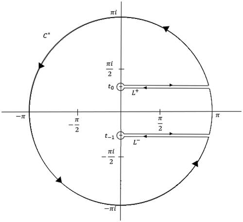
By denoting the loops by $L_{+}$ and $L_{-}$ and the remaining part of the circle $C_1$ by $C^{*},$ we obtain (8) $$\mathit{\text{Res}}[f(w),0]=\frac{n!}{2\pi i}\left({\int }_{C^{*}}f(w)\mathit{\text{dw}}+{\int }_{L^{-}}f(w)\mathit{\text{dw}}+{\int }_{L^{+}}f(w)\mathit{\text{dw}}\right)$$(8) (see Figure 1 to visualize the contour of integration). By the principle of deformation of paths, (9) $$\mathit{\text{Res}}[f(w),0]=\frac{n!}{2\pi i}{\int }_C{\left(\frac{2}{e^{2w}+1}\right)}^{\mu }{e}^{\mathit{\text{wz}}}\frac{\mathit{\text{dw}}}{w^{n+1}}=T_n^{\mu }(z)$$(9) where C is a circle with radius $<\pi /2,$ then Eqs. (8)(8) $$\mathit{\text{Res}}[f(w),0]=\frac{n!}{2\pi i}\left({\int }_{C^{*}}f(w)\mathit{\text{dw}}+{\int }_{L^{-}}f(w)\mathit{\text{dw}}+{\int }_{L^{+}}f(w)\mathit{\text{dw}}\right)$$(8) and (9)(9) $$\mathit{\text{Res}}[f(w),0]=\frac{n!}{2\pi i}{\int }_C{\left(\frac{2}{e^{2w}+1}\right)}^{\mu }{e}^{\mathit{\text{wz}}}\frac{\mathit{\text{dw}}}{w^{n+1}}=T_n^{\mu }(z)$$(9) yield (10) $$T_n^{\mu }(z)=\frac{n!}{2\pi i}\left({\int }_{C^{*}}f(w)\mathit{\text{dw}}+{\int }_{L^{-}}f(w)\mathit{\text{dw}}+{\int }_{L^{+}}f(w)\mathit{\text{dw}}\right).$$(10)

Figure 1. Contour for tangent polynomials of complex order.

Lemma 2.1.

As $n\to \infty$, the integral along $C^{*}$ is $\mathcal{O}({(\pi )}^{-n})$. That is, $${\int }_{C^{*}}f(w)\mathit{\text{dw}}=\mathcal{O}({(\pi )}^{-n}).$$

Proof.

Let $$f(w)={\left(\frac{2}{e^{2w}+1}\right)}^{\mu }\frac{e^{\mathit{\text{wz}}}}{w^{n+1}}$$

where $\mu$ and z are fixed complex numbers. Let $\mathrm{\text{max}}\left\{\right|\mu |,|z\left|\right\}\le K.$ Then (11) $$\left|{\int }_{C^{*}}f(w)\mathit{\text{dw}}\right|<\frac{2^K}{{(\pi )}^{n+1}}{\int }_{C^{*}}|\mathit{\text{dw}}|=\frac{2^K\pi }{{(\pi )}^{n+1}}=\mathcal{O}({(\pi )}^{-n}).$$(11)

Consequently, we have the following theorem.

Theorem 2.2.

As $n\to \infty ,\mu$ and z are fixed complex numbers, (12) $$\begin{array}{cc}{T}_n^{\mu }(z)\sim \frac{n!2^{n+\mu +1}{n}^{\mu -1}}{{\pi }^{n+\mu }\Gamma (\mu )}\{\hspace{0.17em}\mathrm{\text{cos}}\hspace{0.17em}\beta \sum _{k=0}^{\infty }\frac{<1-\mu {>}_k}{n^k}\mathit{\text{Re}}(F_k)\hfill & \hfill \\ -\hspace{0.17em}\mathrm{\text{sin}}\hspace{0.17em}\beta \sum _{k=0}^{\infty }\frac{<1-\mu {>}_k}{n^k}\mathit{\text{Im}}(F_k).\}\hfill & \hfill \end{array}$$(12)

Proof.

For integrals along the loops, let $I_{+}$ be the integral along $L_{+}$ and $I_{-}$ be the integral along $L_{-}.$ To compute these integrals, start with $I_{+}$ $$T_{+}=\frac{n!}{2\pi i}{\int }_{L^{+}}\frac{2^{\mu }{e}^{\mathit{\text{wz}}}}{{(e^{2w}+1)}^{\mu }}\frac{\mathit{\text{dw}}}{w^{n+1}}$$ and let $w=\frac{\pi i{e}^s}{2}.$ Then $\mathit{\text{dw}}=\frac{\pi i{e}^s}{2}\mathit{\text{ds}}$ and $$\begin{array}{ll}{I}_{+}=\frac{n!2^{\mu }}{2\pi i}{\int }_{C^{+}}\frac{\hspace{0.17em}\mathrm{\text{exp}}\left[\frac{\pi \mathit{\text{iz}}{e}^s}{2}\right]}{{(\hspace{0.17em}\mathrm{\text{exp}}[\pi i{e}^s]+1)}^{\mu }}\frac{\frac{\pi i{e}^s\mathit{\text{ds}}}{2}}{{\left(\frac{\pi i{e}^s}{2}\right)}^{n+1}}\hfill & \hfill \\ =\frac{n!2^{\mu }}{2\pi i}{\int }_{C^{+}}\frac{\hspace{0.17em}\mathrm{\text{exp}}\left[\frac{\pi \mathit{\text{iz}}{e}^s}{2}\right]}{{(\hspace{0.17em}\mathrm{\text{exp}}[\pi i{e}^s]+1)}^{\mu }}\frac{\mathit{\text{ds}}}{{\left(\frac{\pi i{e}^s}{2}\right)}^n}\hfill & \hfill \\ =\frac{n!2^{\mu +n}}{2\pi i}{\int }_{C^{+}}\frac{\hspace{0.17em}\mathrm{\text{exp}}\left[\frac{\pi \mathit{\text{iz}}{e}^s}{2}\right]}{{(\hspace{0.17em}\mathrm{\text{exp}}[\pi i{e}^s]+1)}^{\mu }}\frac{\mathit{\text{ds}}}{{(\pi i{e}^s)}^n}.\hfill & \hfill \end{array}$$

Now since $e^{\pi i}=\hspace{0.17em}\mathrm{\text{cos}}\hspace{0.17em}\pi +i\hspace{0.17em}\mathrm{\text{sin}}\hspace{0.17em}\pi =-1,$ then $$I_{+}=\frac{n!2^{\mu +n}}{2\pi i}{\int }_{C^{+}}\frac{e^{\frac{\pi \mathit{\text{iz}}{e}^s}{2}}}{{[e^{\pi i}(e^{\pi i{e}^s}{e}^{-\pi i}-1)]}^{\mu }}\frac{\mathit{\text{ds}}}{{(\pi i{e}^s)}^n}$$ where $C_{+}$ is the image of $L_{+}$ under the transformation $w=\frac{\pi i{e}^s}{2}.C_{+}$ is the contour that encircles the origin in the clockwise direction. Multiplying the numerator by $e^{\frac{-\pi \mathit{\text{iz}}}{2}}{e}^{\frac{\pi \mathit{\text{iz}}}{2}}.$ $$\begin{array}{ll}{I}_{+}=\frac{n!2^{\mu +n}}{2\pi i}{\int }_{C^{+}}\frac{e^{\frac{\pi \mathit{\text{iz}}{e}^s}{2}}{e}^{\frac{-\pi \mathit{\text{iz}}}{2}}{e}^{\frac{\pi \mathit{\text{iz}}}{2}}}{{(e^{\pi i})}^{\mu }{(e^{\pi i{e}^s}{e}^{-\pi i}-1)}^{\mu }}\frac{\mathit{\text{ds}}}{{(\pi i)}^n{e}^{\mathit{\text{sn}}}}\hfill & \hfill \\ =\frac{n!2^{\mu +n}{e}^{-\pi i\mu }{e}^{\frac{\pi \mathit{\text{iz}}}{2}}}{2{(\pi i)}^{n+1}}{\int }_{C^{+}}\frac{e^{\frac{\pi \mathit{\text{iz}}{e}^s}{2}}{e}^{\frac{-\pi \mathit{\text{iz}}}{2}}}{{(e^{\pi i{e}^s}{e}^{-\pi i}-1)}^{\mu }}\frac{\mathit{\text{ds}}}{e^{\mathit{\text{sn}}}}\hfill & \hfill \\ =\frac{n!2^{\mu +n}{e}^{(\frac{z}{2}-\mu )\pi i}}{2{(\pi i)}^{n+1}}{\int }_{C^{+}}\frac{e^{(e^s-1)\frac{\pi \mathit{\text{iz}}}{2}}}{{(e^{(e^s-1)\pi i}-1)}^{\mu }}\frac{\mathit{\text{ds}}}{e^{\mathit{\text{sn}}}}\hfill & \hfill \\ =\frac{n!2^{\mu +n}{e}^{(\frac{z}{2}-\mu )\pi i}}{2{(\pi i)}^{n+1}}{\int }_{C^{+}}\frac{e^{z\nu }}{{(e^{2\nu }-1)}^{\mu }}\frac{\mathit{\text{ds}}}{e^{\mathit{\text{sn}}}}\hfill & \hfill \end{array}$$ where $\nu =(e^s-1)\frac{\pi i}{2}.$ Multiplying the numerator in the last array by $s^{-\mu }{s}^{\mu },$ $$\begin{array}{ll}{I}_{+}=\frac{n!2^{\mu +n}{e}^{(\frac{z}{2}-\mu )\pi i}}{2{(\pi i)}^{n+1}}{\int }_{C^{+}}\frac{e^{z\nu }}{{(e^{2\nu }-1)}^{\mu }}\frac{\mathit{\text{ds}}}{e^{\mathit{\text{sn}}}}{s}^{-\mu }{s}^{\mu }\frac{{(\pi i)}^{\mu }}{{(\pi i)}^{\mu }}\hfill & \hfill \\ =\frac{n!2^{\mu +n}{e}^{(\frac{z}{2}-\mu )\pi i}}{2{(\pi i)}^{n+\mu +1}}{\int }_{C^{+}}{\left(\frac{\pi i}{e^{2\nu }-1}\right)}^{\mu }{e}^{z\nu -\mathit{\text{sn}}}{s}^{-\mu }{s}^{\mu }\mathit{\text{ds}}\hfill & \hfill \\ =\frac{n!2^{\mu +n}{e}^{(\frac{z}{2}-\mu )\pi i}}{2{(\pi i)}^{n+\mu +1}}{\int }_{C^{+}}{\left(\frac{\pi \mathit{\text{is}}}{e^{2\nu }-1}\right)}^{\mu }{e}^{z\nu -\mathit{\text{sn}}}{s}^{-\mu }\mathit{\text{ds}}.\hfill & \hfill \end{array}$$

Now, let $$F(s)={\left(\frac{\pi \mathit{\text{is}}}{e^{2\nu }-1}\right)}^{\mu }{e}^{z\nu }.$$

Then (13) $$I_{+}=\frac{n!2^{\mu +n}{e}^{(\frac{z}{2}-\mu )\pi i}}{2{(\pi i)}^{n+\mu +1}}{\int }_{C^{+}}F(s)e^{-\mathit{\text{ns}}}{s}^{-\mu }\mathit{\text{ds}}.$$(13)

Note that $$\begin{array}{ll}F(s)={\left(\frac{\pi \mathit{\text{is}}}{e^{2\nu }-1}\right)}^{\mu }{e}^{z\nu }\hfill & \hfill \\ ={\left[\frac{\pi \mathit{\text{is}}}{e^{(e^s-1)\pi i}-1}\right]}^{\mu }{e}^{(e^s-1)\frac{\pi \mathit{\text{iz}}}{2}}\hfill & \hfill \\ F(0)=\underset{s\to 0}{\mathrm{\text{lim}}}\left\{{\left[\frac{\pi \mathit{\text{is}}}{e^{(e^s-1)\pi i}-1}\right]}^{\mu }{e}^{(e^s-1)\frac{\pi \mathit{\text{iz}}}{2}}\right\}\hfill & \hfill \\ ={\left[\underset{s\to 0}{\mathrm{\text{lim}}}\frac{\pi \mathit{\text{is}}}{e^{(e^s-1)\pi i}-1}\right]}^{\mu }\left[\underset{s\to 0}{\mathrm{\text{lim}}}{e}^{(e^s-1)\frac{\mathit{\text{piiz}}}{2}}\right]\hfill & \hfill \\ ={\left[\underset{s\to 0}{\mathrm{\text{lim}}}\frac{\pi i}{e^{(e^s-1)\pi i}\pi i{e}^s}\right]}^{\mu }\cdot e^{(e^0-1)\frac{\pi \mathit{\text{iz}}}{2}}\hfill & \hfill \\ =1.\hfill & \hfill \end{array}$$ Applying Watson’s Lemma for loop integrals and then expand, (14) $$F(s)=\sum _{k=0}^{\infty }{F}_k{s}^k.$$(14)

Substituting Eq. (14)(14) $$F(s)=\sum _{k=0}^{\infty }{F}_k{s}^k.$$(14) to (13)(13) $$I_{+}=\frac{n!2^{\mu +n}{e}^{(\frac{z}{2}-\mu )\pi i}}{2{(\pi i)}^{n+\mu +1}}{\int }_{C^{+}}F(s)e^{-\mathit{\text{ns}}}{s}^{-\mu }\mathit{\text{ds}}.$$(13) , then $I_{+}$ becomes $$\begin{array}{ll}{I}_{+}=\frac{n!2^{n+\mu }{e}^{(\frac{z}{2}-\mu )\pi i}}{2{(\pi i)}^{n+\mu +1}}{\int }_{C^{+}}\sum _{k=0}^{\infty }{F}_k{s}^k{e}^{-\mathit{\text{ns}}}{s}^{-\mu }\mathit{\text{ds}}\hfill & \hfill \\ =\frac{n!2^{n+\mu }{e}^{(\frac{z}{2}-\mu )\pi i}}{2{(\pi i)}^{n+\mu +1}}\sum _{k=0}^{\infty }{F}_k{\int }_{C^{+}}{s}^k{e}^{-\mathit{\text{ns}}}{s}^{-\mu }\mathit{\text{ds}}\hfill & \hfill \\ =\frac{n!2^{n+\mu }{e}^{(\frac{z}{2}-\mu )\pi i}}{{(\pi i)}^{n+\mu }}\sum _{k=0}^{\infty }{F}_k{\int }_{C^{+}}\frac{s^{k-\mu }{e}^{-\mathit{\text{ns}}}\mathit{\text{ds}}}{2\pi i}\hfill & \hfill \\ =\frac{n!2^{n+\mu }{e}^{(\frac{z}{2}-\mu )\pi i}}{{(\pi i)}^{n+\mu }}\sum _{k=0}^{\infty }{F}_k{\int }_{C^{+}}\frac{{(-n)}^{-\mu +k}{s}^{k-\mu }{e}^{-\mathit{\text{ns}}}\mathit{\text{ds}}}{2\pi i{(-n)}^{-\mu +k}}\hfill & \hfill \\ =\frac{n!2^{n+\mu }{e}^{(\frac{z}{2}-\mu )\pi i}}{{(\pi i)}^{n+\mu }}\sum _{k=0}^{\infty }{F}_k{\int }_{C^{+}}\frac{{(-\mathit{\text{ns}})}^{-(\mu -k)}{e}^{-\mathit{\text{ns}}}\mathit{\text{ds}}}{2\pi i{(-n)}^{k-\mu }}\hfill & \hfill \\ =\frac{n!2^{n+\mu }{e}^{(\frac{z}{2}-\mu )\pi i}}{{(\pi i)}^{n+\mu }}\sum _{k=0}^{\infty }{F}_k{H}_k\hfill & \hfill \end{array}$$ where (15) $$H_k=\frac{1}{{(-n)}^{k-\mu }}\frac{1}{2\pi i}{\int }_{C^{+}}{e}^{-\mathit{\text{ns}}}{(-\mathit{\text{ns}})}^{-(\mu -k)}\mathit{\text{ds}}.$$(15)

Now, evaluate $H_k.$ Let $t=\mathit{\text{ns}}$ then $\mathit{\text{dt}}=\mathit{\text{nds}},s=\frac{t}{n},\mathit{\text{ds}}=\frac{\mathit{\text{dt}}}{n}$ $$\begin{array}{ll}{H}_k=\frac{1}{{(-n)}^{k-\mu }}\frac{1}{2\pi i}{\int }_{C^{+}}{e}^{-\mathit{\text{ns}}}{(-\mathit{\text{ns}})}^{-(\mu -k)}\mathit{\text{ds}}\hfill & \hfill \\ =\frac{1}{{(-n)}^{k-\mu }}\frac{1}{2\pi i}{\int }_{C^{+}}{e}^{-n\left(\frac{t}{n}\right)}{\left(-n\left(\frac{t}{n}\right)\right)}^{-(\mu -k)}\frac{\mathit{\text{dt}}}{n}\hfill & \hfill \\ =\frac{1}{{(-n)}^{k-\mu +1}}\frac{1}{2\pi i}{\int }_{C^{+}}{e}^{-t}{(-t)}^{-(\mu -k)}\mathit{\text{dt}}.\hfill & \hfill \end{array}$$

By deformation of Paths, and using the reciprocal Gamma function, $$\frac{1}{\Gamma (z)}=\frac{i}{2\pi }{\int }_H{e}^{-t}{(-t)}^{-z}\mathit{\text{dt}}$$ where H is the Hankel contour. Then $$\begin{array}{ll}{H}_k=-\frac{1}{{(-n)}^{k-\mu +1}}\frac{i}{2\pi }{\int }_H{e}^{-t}{(-t)}^{-(\mu -k)}\mathit{\text{dt}}\hfill & \hfill \\ =-\frac{1}{{(-n)}^{k-\mu +1}}\frac{1}{\Gamma (\mu -k)}\hfill & \hfill \\ =(-1){(-n)}^{\mu -k-1}\frac{1}{\Gamma (\mu -k)}\hfill & \hfill \\ ={(-1)}^{\mu -k}{(n)}^{\mu -k-1}\frac{1}{\Gamma (\mu -k)}.\hfill & \hfill \end{array}$$

Moreover, $$\begin{array}{ll}{H}_k={(-1)}^{\mu }{(-1)}^{-k}{n}^{\mu -k-1}\frac{1}{\Gamma (\mu -k)}\hfill & \hfill \\ ={(-1)}^{\mu }{(-1)}^k{n}^{\mu -k-1}\frac{1}{\Gamma (\mu -k)}\hfill & \hfill \\ =e^{\pi i\mu }{n}^{\mu -k-1}\frac{{(-1)}^k}{\Gamma (\mu -k)}\hfill & \hfill \end{array}$$ and $\Gamma (\mu -k)=(\mu -k-1)!.$ Then $$\begin{array}{ll}\frac{{(-1)}^k}{\Gamma (\mu -k)}=\frac{{(-1)}^k}{(\mu -k-1)!}\hfill & \hfill \\ =\frac{{(-1)}^k(\mu -1)(\mu -2)(\mu -3)\cdots (\mu -k)}{(\mu -1)!}\hfill & \hfill \\ =\frac{{(-1)}^k(\mu -1)(\mu -2)(\mu -3)\cdots (\mu -k)}{\Gamma (\mu )}\hfill & \hfill \\ =\frac{<1-\mu {>}_k}{\Gamma (\mu )}\hfill & \hfill \end{array}$$ since $$\begin{array}{cc}<x{>}_k\hfill & =x(x+1)(x+2)\cdots (x+k-1)\hfill \\ <1-\mu {>}_k\hfill & =(1-\mu )(2-\mu )(3-\mu )\cdots (k-\mu )\hfill \end{array}$$

Thus, $$H_k=n^{\mu -k-1}{e}^{\pi i\mu }\frac{<1-\mu {>}_k}{\Gamma (\mu )}.$$

Writing $i^{n+\mu }=e^{(n+\mu )\frac{\pi i}{2}}$ $$\begin{array}{ll}{I}_{+}=\frac{n!2^{n+\mu }{e}^{\left(\frac{z}{2}-\mu \right)\pi i}}{{(\pi i)}^{n+\mu }}\sum _{k=0}^{\infty }{F}_k{H}_k\hfill & \hfill \\ =\frac{n!2^{n+\mu }{e}^{\left(\frac{z}{2}-\mu \right)\pi i}}{{(\pi i)}^{n+\mu }}\sum _{k=0}^{\infty }{F}_k{n}^{\mu -k-1}{e}^{\pi i\mu }\frac{<1-\mu {>}_k}{\Gamma (\mu )}\hfill & \hfill \\ =\frac{n!2^{n+\mu }{e}^{\frac{z}{2}\pi i}{n}^{\mu -1}}{{\pi }^{n+\mu }{(i)}^{n+\mu }\Gamma (\mu )}\sum _{k=0}^{\infty }{F}_k\frac{<1-\mu {>}_k}{n^k}\hfill & \hfill \\ =\frac{n!2^{n+\mu }{e}^{-(n+\mu )\frac{\pi i}{2}}{e}^{\frac{z}{2}\pi i}{n}^{\mu -1}}{{\pi }^{n+\mu }\Gamma (\mu )}\sum _{k=0}^{\infty }{F}_k\frac{<1-\mu {>}_k}{n^k}\hfill & \hfill \\ =\frac{n!2^{n+\mu }{e}^{(z-n-\mu )\frac{z}{2}\pi i}{n}^{\mu -1}}{{\pi }^{n+\mu }\Gamma (\mu )}\sum _{k=0}^{\infty }{F}_k\frac{<1-\mu {>}_k}{n^k}.\hfill & \hfill \end{array}$$

Since $e^{(z-n-\mu )\frac{\pi i}{2}}=\hspace{0.17em}\mathrm{\text{cos}}\hspace{0.17em}\left[(z-n-\mu )\frac{\pi }{2}\right]+i\hspace{0.17em}\mathrm{\text{sin}}\hspace{0.17em}\left[(z-n-\mu )\frac{\pi }{2}\right],$ then $$\begin{array}{ll}{I}_{+}=\frac{n!2^{n+\mu }{n}^{\mu -1}}{{\pi }^{n+\mu }\Gamma (\mu )}(\hspace{0.17em}\mathrm{\text{cos}}\hspace{0.17em}\beta +i\hspace{0.17em}\mathrm{\text{sin}}\hspace{0.17em}\beta )[\sum _{k=0}^{\infty }\frac{<1-\mu {>}_k}{n^k}\mathit{\text{Re}}(F_k)+i\sum _{k=0}^{\infty }\frac{<1-\mu {>}_k}{n^k}\mathit{\text{Im}}(F_k)]\hfill & \hfill \\ =\frac{n!2^{n+\mu }{n}^{\mu -1}}{{\pi }^{n+\mu }\Gamma (\mu )}[\mathrm{\text{cos}}\hspace{0.17em}\beta \sum _{k=0}^{\infty }\frac{<1-\mu {>}_k}{n^k}\mathit{\text{Re}}(F_k)+i\hspace{0.17em}\mathrm{\text{sin}}\hspace{0.17em}\beta \sum _{k=0}^{\infty }\frac{<1-\mu {>}_k}{n^k}\mathit{\text{Re}}(F_k)\hfill & \hfill \\ +i\hspace{0.17em}\mathrm{\text{cos}}\hspace{0.17em}\beta \sum _{k=0}^{\infty }\frac{<1-\mu {>}_k}{n^k}\mathit{\text{Im}}(F_k)-\hspace{0.17em}\mathrm{\text{sin}}\hspace{0.17em}\beta \sum _{k=0}^{\infty }\frac{<1-\mu {>}_k}{n^k}\mathit{\text{Im}}(F_k)]\hfill & \hfill \end{array}$$ where $\beta =(z-n-\mu )\frac{\pi }{2}.$

The integral along $L_{-}$ denoted by $I_{-}$ can be obtained similarly, with $w=-\frac{\pi i{e}^s}{2}.$ It can be shown that $I_{-}$ is the complex conjugate of $I_{+}$ (not considering z and $\mu$ as complex numbers). Thus, Eq. (10)(10) $$T_n^{\mu }(z)=\frac{n!}{2\pi i}\left({\int }_{C^{*}}f(w)\mathit{\text{dw}}+{\int }_{L^{-}}f(w)\mathit{\text{dw}}+{\int }_{L^{+}}f(w)\mathit{\text{dw}}\right).$$(10) given $$T_n^{\mu }(z)\sim I_{+}+I_{-}=2\mathit{\text{Re}}(I_{+}).$$ hence, $$T_n^{\mu }(z)=\frac{n!2^{n+\mu +1}{n}^{\mu -1}}{{\pi }^{n+\mu }\Gamma (\mu )}[\mathrm{\text{cos}}\hspace{0.17em}\beta \sum _{k=0}^{\infty }\frac{<1-\mu {>}_k}{n^k}\mathit{\text{Re}}(F_k)-\hspace{0.17em}\mathrm{\text{sin}}\hspace{0.17em}\beta \sum _{k=0}^{\infty }\frac{<1-\mu {>}_k}{n^k}\mathit{\text{Im}}(F_k)]$$

The first order approximation is given by the following theorem,

Lemma 2.3.

As $n\to \infty ,\mu$ and z are fixed numbers, $$T_n^{\mu }(z)\sim \frac{n!2^{n+\mu +1}{n}^{\mu -1}}{{\pi }^{n+\mu }\Gamma (\mu )}\left\{\hspace{0.17em}\mathrm{\text{cos}}\hspace{0.17em}\beta +\mathcal{O}\left(\frac{1}{n}\right)\right\}$$ where $\beta =(z-n-\mu )\frac{\pi }{2}.$

Proof.

Let us consider the first term of the sum in Eq. (12)(12) $$\begin{array}{cc}{T}_n^{\mu }(z)\sim \frac{n!2^{n+\mu +1}{n}^{\mu -1}}{{\pi }^{n+\mu }\Gamma (\mu )}\{\hspace{0.17em}\mathrm{\text{cos}}\hspace{0.17em}\beta \sum _{k=0}^{\infty }\frac{<1-\mu {>}_k}{n^k}\mathit{\text{Re}}(F_k)\hfill & \hfill \\ -\hspace{0.17em}\mathrm{\text{sin}}\hspace{0.17em}\beta \sum _{k=0}^{\infty }\frac{<1-\mu {>}_k}{n^k}\mathit{\text{Im}}(F_k).\}\hfill & \hfill \end{array}$$(12) . Note that $F_0=F(0)=1.$ Then, $$\begin{array}{ll}{T}_n^{\mu }(z)\sim \frac{n!2^{n+\mu +1}{n}^{\mu -1}}{{\pi }^{n+\mu }\Gamma (\mu )}\left[\left(\hspace{0.17em}\mathrm{\text{cos}}\hspace{0.17em}\beta \right)\left(\mathit{\text{Re}}(F_0)\right)-\left(\hspace{0.17em}\mathrm{\text{sin}}\hspace{0.17em}\beta \right)\left(\mathit{\text{Im}}(F_0)\right)\right]\hfill & \hfill \\ \sim \frac{n!2^{n+\mu +1}{n}^{\mu -1}}{{\pi }^{n+\mu }\Gamma (\mu )}\left[(\hspace{0.17em}\mathrm{\text{cos}}\hspace{0.17em}\beta )(1)-(\hspace{0.17em}\mathrm{\text{sin}}\hspace{0.17em}\beta )(0)\right]\hfill & \hfill \\ \sim \frac{n!2^{n+\mu +1}{n}^{\mu -1}}{{\pi }^{n+\mu }\Gamma (\mu )}\left[\mathrm{\text{cos}}\hspace{0.17em}\beta +\mathcal{O}\left(\frac{1}{n}\right)\right]\hfill & \hfill \end{array}$$

3. Alternative expansion for Tangent polynomials

In this section, an alternative approach is employed to derive an asymptotic representation of the integral defined in Eq. (1)(1) $${\left(\frac{2}{e^{2w}+1}\right)}^{\mu }{e}^{\mathit{\text{wz}}}=\sum _{n=0}^{\infty }{T}_n^{\mu }(z)\frac{w^n}{n!},\left|w\right|<\frac{\pi }{2}.$$(1) . By expanding the integrand using a two-point Taylor expansion, we can unveil a different expression that captures the behavior of the integral. This method allows us to explore the integral’s behavior in a different mathematical framework, potentially offering new insights or perspectives on its properties.

Now, let $$\begin{array}{ll}g(w)={\left(\frac{w^2+{\left(\frac{\pi }{2}\right)}^2}{\pi }\right)}^{\mu }{\left(\frac{2}{e^{2w}+1}\right)}^{\mu }{e}^{\mathit{\text{wz}}}\hfill & \hfill \\ ={\left(\frac{w^2+{\left(\frac{\pi }{2}\right)}^2}{e^{2w}+1}\right)}^{\mu }{\left(\frac{2}{\pi }\right)}^{\mu }{e}^{\mathit{\text{wz}}}\hfill & \hfill \\ g\left(\frac{\pi i}{2}\right)={\left(\frac{2\left(\frac{\pi i}{2}\right)}{2e^{\pi i}}\right)}^{\mu }{\left(\frac{2}{\pi }\right)}^{\mu }{e}^{\frac{\pi \mathit{\text{iz}}}{2}}={(-i)}^{\mu }{e}^{\frac{\pi \mathit{\text{iz}}}{2}}\hfill & \hfill \end{array}$$ and expand $$g(w)=\sum _{k=0}^{\infty }({\alpha }_k+w{\beta }_k){\left(w^2+{\left(\frac{\pi }{2}\right)}^2\right)}^k$$ all are zero except when $k=0,$ then $$g\left(\frac{\pi i}{2}\right)+g\left(-\frac{\pi i}{2}\right)={\alpha }_0+\frac{\pi i}{2}{\beta }_0+{\alpha }_0-\frac{\pi i}{2}{\beta }_0=2{\alpha }_0$$ hence, $$\frac{g\left(\frac{\pi i}{2}\right)+g\left(-\frac{\pi i}{2}\right)}{2}={\alpha }_0.$$

On the other hand, $$g\left(\frac{\pi i}{2}\right)+g\left(-\frac{\pi i}{2}\right)={\alpha }_0+\frac{\pi i}{2}{\beta }_0-{\alpha }_0+\frac{\pi i}{2}{\beta }_0=\pi i{\beta }_0$$ hence, $$\frac{g\left(\frac{\pi i}{2}\right)-g\left(-\frac{\pi i}{2}\right)}{2}={\beta }_0.$$

Computing $g\left(-\frac{\pi i}{2}\right),$ $$g\left(-\frac{\pi i}{2}\right)=\left(\frac{2\left(-\frac{\pi i}{2}\right)}{2e^{-\pi i}}\right){\left(\frac{2}{\pi }\right)}^{\mu }{e}^{-\frac{\pi \mathit{\text{iz}}}{2}}=i^{\mu }{e}^{-\frac{\pi \mathit{\text{iz}}}{2}}.$$

Hence, $$\begin{array}{ll}{\alpha }_0=\frac{g\left(\frac{\pi i}{2}\right)+g(-\frac{\pi i}{2})}{2}\hfill & \hfill \\ =\frac{{(-i)}^{\mu }{e}^{\frac{\pi \mathit{\text{iz}}}{2}}+i^u{e}^{-\frac{\pi \mathit{\text{iz}}}{2}}}{2}\hfill & \hfill \\ =\frac{e^{-\frac{\pi i\mu }{2}}{e}^{\frac{\pi \mathit{\text{iz}}}{2}}+e^{\frac{\pi i\mu }{2}{e}^{-\frac{\pi \mathit{\text{iz}}}{2}}}}{2}\hfill & \hfill \\ =\frac{\hspace{0.17em}\mathrm{\text{cos}}\hspace{0.17em}\left((z-\mu )\frac{\pi }{2}\right)+i\hspace{0.17em}\mathrm{\text{sin}}\hspace{0.17em}\left((z-\mu )\frac{\pi }{2}\right)+\hspace{0.17em}\mathrm{\text{cos}}\hspace{0.17em}\left((z-\mu )\frac{\pi }{2}\right)-i\hspace{0.17em}\mathrm{\text{sin}}\hspace{0.17em}\left((z-\mu )\frac{\pi }{2}\right)}{2}\hfill & \hfill \\ =\frac{2\hspace{0.17em}\mathrm{\text{cos}}\hspace{0.17em}\left((z-\mu )\frac{\pi }{2}\right)}{2}\hfill & \hfill \\ =\hspace{0.17em}\mathrm{\text{cos}}\hspace{0.17em}\left((z-\mu )\frac{\pi }{2}\right)\hfill & \hfill \end{array}$$ and $$\begin{array}{ll}{\beta }_0=\frac{g\left(\frac{\pi i}{2}\right)-g(-\frac{\pi i}{2})}{\pi i}\hfill & \hfill \\ =\frac{{(-i)}^{\mu }{e}^{\frac{\pi \mathit{\text{iz}}}{2}}-i^{\mu }{e}^{-\frac{\pi \mathit{\text{iz}}}{2}}}{\pi i}\hfill & \hfill \\ =\frac{e^{-\frac{\pi i\mu }{2}}{e}^{\frac{\pi \mathit{\text{iz}}}{2}}-e^{\frac{\pi i\mu }{2}}{e}^{-\frac{\pi \mathit{\text{iz}}}{2}}}{\pi i}\hfill & \hfill \\ =\frac{\hspace{0.17em}\mathrm{\text{cos}}\hspace{0.17em}\left((z-\mu )\frac{\pi }{2}\right)+i\hspace{0.17em}\mathrm{\text{sin}}\hspace{0.17em}\left((z-\mu )\frac{\pi }{2}\right)-\hspace{0.17em}\mathrm{\text{cos}}\hspace{0.17em}\left((z-\mu )\frac{\pi }{2}\right)+i\hspace{0.17em}\mathrm{\text{sin}}\hspace{0.17em}\left((z-\mu )\frac{\pi }{2}\right)}{\pi i}\hfill & \hfill \\ =\frac{2i\hspace{0.17em}\mathrm{\text{sin}}\hspace{0.17em}\left((z-\mu )\frac{\pi }{2}\right)}{\pi i}\hfill & \hfill \\ =\frac{2\hspace{0.17em}\mathrm{\text{sin}}\hspace{0.17em}\left((z-\mu )\frac{\pi }{2}\right)}{\pi }\hfill & \hfill \end{array}$$

To be able to compute the values ${\alpha }_j$ and ${\beta }_j,$ for j other than 0, we proceed as follows: $$\begin{array}{ll}g(w)\hfill & =({\alpha }_0+w{\beta }_0)+({\alpha }_1+w{\beta }_1)\left(w^2+{\left(\frac{\pi }{2}\right)}^2\right)+({\alpha }_2+w{\beta }_2){\left(w^2+{\left(\frac{\pi }{2}\right)}^2\right)}^2+\dots \hfill \\ g(w)-({\alpha }_0+w{\beta }_0)\hfill & =\left(w^2+{\left(\frac{\pi }{2}\right)}^2\right)g_1(w)\hfill \end{array}$$ where (16) $$g_1(w)=({\alpha }_1+w{\beta }_1)+({\alpha }_2+w{\beta }_2)\left(w^2+{\left(\frac{\pi }{2}\right)}^2\right)+({\alpha }_3+w{\beta }_3){\left(w^2+{\left(\frac{\pi }{2}\right)}^2\right)}^2+\dots$$(16) $$\begin{array}{ll}{g}_1(w)-({\alpha }_1+w{\beta }_1)\hfill & =\left(w^2+{\left(\frac{\pi }{2}\right)}^2\right)g_2(w)\hfill \\ g_2(w)-({\alpha }_2+w{\beta }_2)\hfill & =\left(w^2+{\left(\frac{\pi }{2}\right)}^2\right)g_3(w)\hfill \\ \hfill \hspace{1em}\hspace{1em}\hspace{1em}\hspace{1em}\hspace{1em}\hspace{1em}\hspace{1em}\hspace{1em}·\hfill & \hfill \\ \hspace{1em}\hspace{1em}\hspace{1em}\hspace{1em}\hspace{1em}\hspace{1em}\hspace{1em}\hspace{1em}·\hfill & \hfill \\ \hspace{1em}\hspace{1em}\hspace{1em}\hspace{1em}\hspace{1em}\hspace{1em}\hspace{1em}\hspace{1em}·\hfill & \hfill \\ g_j(w)-({\alpha }_j+w{\beta }_j)\hfill & =\left(w^2+{\left(\frac{\pi }{2}\right)}^2\right)g_{j+1}(w)\hfill \end{array}$$ hence, $$\begin{array}{ll}{g}_{j+1}(w)=\frac{g_j(w)-({\alpha }_j+w{\beta }_j)}{w^2+{(\frac{\pi }{2})}^2}\hfill & \hfill \\ =\sum _{k=j+1}({\alpha }_{j+1}+w{\beta }_{j+1}){\left(w^2+{\left(\frac{\pi }{2}\right)}^2\right)}^{k-(j+1)}\hfill & \hfill \end{array}$$

Taking the limit as $w\to \frac{\pi i}{2},$ $$\begin{array}{ll}\underset{w\to \frac{\pi i}{2}}{\mathrm{\text{lim}}}{g}_{j+1}(w)=\underset{w\to \frac{\pi i}{2}}{\mathrm{\text{lim}}}\frac{g_j(w)-({\alpha }_j+w{\beta }_j)}{(w^2+{(\frac{\pi }{2})}^2)}\hfill & \hfill \\ =\underset{w\to \frac{\pi i}{2}}{\mathrm{\text{lim}}}\frac{g_j(w)-{\beta }_j}{(2w)}\hfill & \hfill \\ =\frac{g_j\left(\frac{\pi i}{2}\right)-{\beta }_j}{\pi i}.\hfill & \hfill \end{array}$$

Since, $$\begin{array}{ll}{g}_{j+1}(w)\hfill & =\sum _{k=j+1}^{\infty }({\alpha }_k+w{\beta }_k){\left(w^2+{\left(\frac{\pi }{2}\right)}^2\right)}^{k-j-1}\hfill \\ g_{j+1}\left(\frac{\pi i}{2}\right)\hfill & =\sum _{k=j+1}^{\infty }({\alpha }_k+\frac{\pi i}{2}{\beta }_k){\left({\left(\frac{\pi i}{2}\right)}^2+{\left(\frac{\pi }{2}\right)}^2\right)}^{k-j-1}\hfill \end{array}$$ and all are zero except when $k=j+1,$ then $$g_{j+1}\left(\frac{\pi i}{2}\right)={\alpha }_{j+1}+\frac{\pi i}{2}{\beta }_{j+1}.$$

Thus, (17) $$\begin{array}{ll}{\alpha }_{j+1}+\frac{\pi i}{2}{\beta }_{j+1}\hfill & =\frac{g_j\left(\frac{\pi i}{2}\right)-{\beta }_j}{\pi i}\hfill \\ \pi i{\alpha }_{j+1}-\frac{{\pi }^2}{2}{\beta }_{j+1}\hfill & =g_j\left(\frac{\pi i}{2}\right)-{\beta }_j.\hfill \end{array}$$(17)

On the other hand, $$\begin{array}{ll}{g}_{j+1}(w)=\underset{w\to -\frac{\pi i}{2}}{\mathrm{\text{lim}}}\frac{g_j(w)-({\alpha }_j+w{\beta }_j)}{w^2+{(\frac{\pi }{2})}^2}\hfill & \hfill \\ =\underset{w\to -\frac{\pi i}{2}}{\mathrm{\text{lim}}}\frac{g_j(w)-{\beta }_j}{2w}\hfill & \hfill \\ =\frac{g_j(-\frac{\pi i}{2})-{\beta }_j}{-\pi i}\hfill & \hfill \end{array}$$ since $$\begin{array}{cc}{g}_{j+1}\left(-\frac{\pi i}{2}\right)=({\alpha }_{j+1}-\frac{\pi i}{2}{\beta }_{j+1}){\left(w^2+{\left(\frac{\pi }{2}\right)}^2\right)}^{j+1-(j+1)}\hfill & \hfill \\ ={\alpha }_{j+1}-\frac{\pi i}{2}{\beta }_{j+1},\hfill & \hfill \end{array}$$ hence, (18) $$\begin{array}{cc}{\alpha }_{j+1}-\frac{\pi i}{2}{\beta }_{j+1}\hfill & =\frac{g_j(-\frac{\pi i}{2})-{\beta }_j}{-\pi i}\hfill \\ -\pi i{\alpha }_{j+1}-\frac{{\pi }^2}{2}{\beta }_{j+1}\hfill & =\frac{g_j(-\frac{\pi i}{2})-{\beta }_j}{-\pi i}.\hfill \end{array}$$(18)

Adding Eqs. (17)(17) $$\begin{array}{ll}{\alpha }_{j+1}+\frac{\pi i}{2}{\beta }_{j+1}\hfill & =\frac{g_j\left(\frac{\pi i}{2}\right)-{\beta }_j}{\pi i}\hfill \\ \pi i{\alpha }_{j+1}-\frac{{\pi }^2}{2}{\beta }_{j+1}\hfill & =g_j\left(\frac{\pi i}{2}\right)-{\beta }_j.\hfill \end{array}$$(17) and (18)(18) $$\begin{array}{cc}{\alpha }_{j+1}-\frac{\pi i}{2}{\beta }_{j+1}\hfill & =\frac{g_j(-\frac{\pi i}{2})-{\beta }_j}{-\pi i}\hfill \\ -\pi i{\alpha }_{j+1}-\frac{{\pi }^2}{2}{\beta }_{j+1}\hfill & =\frac{g_j(-\frac{\pi i}{2})-{\beta }_j}{-\pi i}.\hfill \end{array}$$(18) yields, $$\begin{array}{ll}{g}_j\left(\frac{\pi i}{2}\right)-{\beta }_j+g_j\left(\frac{-\pi i}{2}\right)-{\beta }_j\hfill & =\pi i{\alpha }_{j+1}-\frac{{\pi }^2}{2}{\beta }_{j+1}-\pi i{\alpha }_{j+1}-\frac{{\pi }^2}{2}{\beta }_{j+1}\hfill \\ =-{\pi }^2{\beta }_{j+1}.\hfill & \hfill \end{array}$$

So, (19) $$\begin{array}{ll}{g}_j\left(\frac{\pi i}{2}\right)-2{\beta }_j+g_j\left(-\frac{\pi i}{2}\right)\hfill & =-{\pi }^2{\beta }_{j+1}\hfill \\ \frac{g_j\left(\frac{\pi i}{2}\right)-2{\beta }_j+g_j(-\frac{\pi i}{2})}{-{\pi }^2}=\hfill & {\beta }_{j+1}.\hfill \end{array}$$(19)

Subtracting Eqs. (17)(17) $$\begin{array}{ll}{\alpha }_{j+1}+\frac{\pi i}{2}{\beta }_{j+1}\hfill & =\frac{g_j\left(\frac{\pi i}{2}\right)-{\beta }_j}{\pi i}\hfill \\ \pi i{\alpha }_{j+1}-\frac{{\pi }^2}{2}{\beta }_{j+1}\hfill & =g_j\left(\frac{\pi i}{2}\right)-{\beta }_j.\hfill \end{array}$$(17) and (18)(18) $$\begin{array}{cc}{\alpha }_{j+1}-\frac{\pi i}{2}{\beta }_{j+1}\hfill & =\frac{g_j(-\frac{\pi i}{2})-{\beta }_j}{-\pi i}\hfill \\ -\pi i{\alpha }_{j+1}-\frac{{\pi }^2}{2}{\beta }_{j+1}\hfill & =\frac{g_j(-\frac{\pi i}{2})-{\beta }_j}{-\pi i}.\hfill \end{array}$$(18) yields, $$\begin{array}{ll}{g}_j\left(\frac{\pi i}{2}\right)-{\beta }_j-g_j\left(\frac{\pi i}{2}\right)+{\beta }_j\hfill & =\pi i{\alpha }_{j+1}-\frac{{\pi }^2}{2}{\beta }_{j+1}+\pi i{\alpha }_{j+1}+\frac{{\pi }^2}{2}{\beta }_{j+1}\hfill \\ =2\pi i{\alpha }_{j+1}.\hfill & \hfill \end{array}$$

So, (20) $$\frac{g_j\left(\frac{\pi i}{2}\right)-g_j(-\frac{\pi i}{2})}{2\pi i}={\alpha }_{j+1}$$(20)

Going back to $g(w)$ $$\begin{array}{ll}g(w)={\left(\frac{w^2+\left(\frac{\pi }{2}\right)}{\pi }\right)}^{\mu }{\left(\frac{2}{e^{2w}+1}\right)}^{\mu }{e}^{\mathit{\text{wz}}}\hfill & \hfill \\ =\sum _{k=0}^{\infty }({\alpha }_k+w{\beta }_k){\left(w^2+{\left(\frac{\pi }{2}\right)}^2\right)}^k,\hfill & \hfill \end{array}$$ then (21) $$\begin{array}{ll}{\left(\frac{2}{e^{2w}+1}\right)}^{\mu }{e}^{\mathit{\text{wz}}}={\left(\frac{\pi }{w^2+{(\frac{\pi }{2})}^2}\right)}^{\mu }\sum _{k=0}^{\infty }({\alpha }_k+w{\beta }_k){\left(w^2+{\left(\frac{\pi }{2}\right)}^2\right)}^k\hfill & \hfill \\ =\sum _{k=0}^{\infty }{\pi }^{\mu }({\alpha }_k+w{\beta }_k){\left(w^2+{\left(\frac{\pi }{2}\right)}^2\right)}^{k-\mu }\hfill & \hfill \end{array}$$(21)

Consequently, by substituting Eq. (21)(21) $$\begin{array}{ll}{\left(\frac{2}{e^{2w}+1}\right)}^{\mu }{e}^{\mathit{\text{wz}}}={\left(\frac{\pi }{w^2+{(\frac{\pi }{2})}^2}\right)}^{\mu }\sum _{k=0}^{\infty }({\alpha }_k+w{\beta }_k){\left(w^2+{\left(\frac{\pi }{2}\right)}^2\right)}^k\hfill & \hfill \\ =\sum _{k=0}^{\infty }{\pi }^{\mu }({\alpha }_k+w{\beta }_k){\left(w^2+{\left(\frac{\pi }{2}\right)}^2\right)}^{k-\mu }\hfill & \hfill \end{array}$$(21) to Cauchy Integral Formula of Tangent polynomials, (22) $$\begin{array}{l}{T}_n^{\mu }(z)=\frac{n!}{2\pi i}{\int }_C{\left(\frac{2}{e^{2w}+1}\right)}^{\mu }{e}^{\mathit{\text{wz}}}\frac{\mathit{\text{dw}}}{w^{n+1}}\\ =\frac{n!}{2\pi i}{\int }_C\sum _{k=0}^{\infty }{\pi }^{\mu }({\alpha }_k+w{\beta }_k){\left(w^2+{\left(\frac{\pi }{2}\right)}^2\right)}^{k-\mu }\frac{\mathit{\text{dw}}}{w^{n+1}}\\ ={\pi }^{\mu }n!\sum _{k=0}^{\infty }\frac{1}{2\pi i}{\int }_C({\alpha }_k+w{\beta }_k){\left(w^2+{\left(\frac{\pi }{2}\right)}^2\right)}^{k-\mu }\frac{\mathit{\text{dw}}}{w^{n+1}}\\ ={\pi }^{\mu }n!\left\{\sum _{k=0}^{\infty }\frac{1}{2\pi i}\left[{\int }_C{\alpha }_k{\left(w^2+{\left(\frac{\pi }{2}\right)}^2\right)}^{k-\mu }\frac{\mathit{\text{dw}}}{w^{n+1}}+{\int }_C{\beta }_k{\left(w^2+{\left(\frac{\pi }{2}\right)}^2\right)}^{k-\mu }\frac{\mathit{\text{dw}}}{w^n}\right]\right\}\\ ={\pi }^{\mu }n!\left[\sum _{k=0}^{\infty }\frac{{\alpha }_k}{2\pi i}{\int }_C{\left(w^2+{\left(\frac{\pi }{2}\right)}^2\right)}^{k-\mu }\frac{\mathit{\text{dw}}}{w^{n+1}}+\sum _{k=0}^{\infty }\frac{{\beta }_k}{2\pi i}{\int }_C{\left(w^2+{\left(\frac{\pi }{2}\right)}^2\right)}^{k-\mu }\frac{\mathit{\text{dw}}}{w^n}\right]\\ ={\pi }^{\mu }n!\sum _{k=0}^{\infty }[{\alpha }_k{\Phi }_k^{(n)}+{\beta }_k{\Phi }_k^{(n-1)}]\end{array}$$(22) where (23) $$\begin{array}{ll}{\Phi }_k^{(n)}=\frac{1}{2\pi i}{\int }_C{\left(w^2+{\left(\frac{\pi }{2}\right)}^2\right)}^{k-\mu }\frac{\mathit{\text{dw}}}{w^{n+1}}\hfill & \hfill \\ {\Phi }_k^{(n-1)}=\frac{1}{2\pi i}{\int }_C{\left(w^2+{\left(\frac{\pi }{2}\right)}^2\right)}^{k-\mu }\frac{\mathit{\text{dw}}}{w^n}\hfill & \hfill \\ {\Phi }_k^{(2n+1)}=\frac{1}{2\pi i}{\int }_C{\left(w^2+{\left(\frac{\pi }{2}\right)}^2\right)}^{k-\mu }\frac{\mathit{\text{dw}}}{w^{2n+2}}\hfill & \hfill \\ =\frac{1}{2\pi i}{\int }_C\sum _{j=0}^{k-\mu }\left(\begin{array}{c}k-\mu \\ j\end{array}\right)w^{2j}{\left({\left(\frac{\pi }{2}\right)}^2\right)}^{k-\mu -j}\frac{\mathit{\text{dw}}}{w^{2n+2}}\hfill & \hfill \\ =\sum _{j\ge 0}\left(\begin{array}{c}k-\mu \\ j\end{array}\right)w^{2j}{\left({\left(\frac{\pi }{2}\right)}^2\right)}^{k-\mu -j}\frac{1}{2\pi i}{\int }_C{w}^{2j-2n-2}\mathit{\text{dw}}\hfill & \hfill \\ =0\hfill & \hfill \end{array}$$(23) since $2j-2n-2\ne 1\forall j\ge 0$ and using the fact that $$\begin{array}{c}{\int }_C\frac{\mathit{\text{dz}}}{{(z-z_0)}^n}=\{\begin{array}{cc}2\pi i\hfill & \text{for}n=-1\hfill \\ 0\hfill & \text{for}n\ne -1\hfill \end{array}\hfill \end{array}$$ where C is a circle about $z_0.$ On the other hand, $$\begin{array}{ll}{\Phi }_k^{(2n)}=\frac{1}{2\pi i}{\int }_C\sum _{j\ge 0}\left(\begin{array}{c}k-\mu \\ j\end{array}\right)w^{2j}{\left({\left(\frac{\pi }{2}\right)}^2\right)}^{k-\mu -j}\frac{\mathit{\text{dw}}}{w^{2n+1}}\hfill & \hfill \\ =\sum _{j\ge 0}\left(\begin{array}{c}k-\mu \\ j\end{array}\right){\left(\frac{\pi }{2}\right)}^{2k-2\mu -2j}\frac{1}{2\pi i}{\int }_C{w}^{2j-2n-1}\mathit{\text{dw}}\hfill & \hfill \end{array}$$ when $j=n$ (24) $$\begin{array}{l}=\left(\begin{array}{c}k-\mu \\ n\end{array}\right){\left(\frac{\pi }{2}\right)}^{2k-2\mu -2n}\frac{1}{2\pi i}{\int }_C{w}^{-1}\mathit{\text{dw}}\hfill \\ =\left(\begin{array}{c}k-\mu \\ n\end{array}\right){\left(\frac{\pi }{2}\right)}^{2k-2\mu -2n}\frac{1}{2\pi i}(2\pi i)\hfill \\ =\left(\begin{array}{c}k-\mu \\ n\end{array}\right){\left(\frac{\pi }{2}\right)}^{2k-2\mu -2n}\hfill \\ =\frac{(k-\mu )!}{n!(k-\mu -n)!}{\left(\frac{\pi }{2}\right)}^{2k-2\mu -2n}\hfill \\ =\frac{{(k-\mu )}_n}{n!}{\left(\frac{\pi }{2}\right)}^{2k-2\mu -2n}\hfill \\ ={(-1)}^n\frac{<\mu -k{>}_n}{n!}{\left(\frac{\pi }{2}\right)}^{2k-2\mu -2n}\hfill \end{array}$$(24) where $$\begin{array}{ll}{(k-\mu )}_n=(k-\mu )(k-\mu -1)\cdots (k-\mu -(n-1))\hfill & \hfill \\ ={(-1)}^n(\mu -k)(\mu -k+1)\cdots (\mu -k+(n-1))\hfill & \hfill \\ ={(-1)}^n<\mu -k{>}_n.\hfill & \hfill \end{array}$$

Hence using Eqs. (22)(22) $$\begin{array}{l}{T}_n^{\mu }(z)=\frac{n!}{2\pi i}{\int }_C{\left(\frac{2}{e^{2w}+1}\right)}^{\mu }{e}^{\mathit{\text{wz}}}\frac{\mathit{\text{dw}}}{w^{n+1}}\\ =\frac{n!}{2\pi i}{\int }_C\sum _{k=0}^{\infty }{\pi }^{\mu }({\alpha }_k+w{\beta }_k){\left(w^2+{\left(\frac{\pi }{2}\right)}^2\right)}^{k-\mu }\frac{\mathit{\text{dw}}}{w^{n+1}}\\ ={\pi }^{\mu }n!\sum _{k=0}^{\infty }\frac{1}{2\pi i}{\int }_C({\alpha }_k+w{\beta }_k){\left(w^2+{\left(\frac{\pi }{2}\right)}^2\right)}^{k-\mu }\frac{\mathit{\text{dw}}}{w^{n+1}}\\ ={\pi }^{\mu }n!\left\{\sum _{k=0}^{\infty }\frac{1}{2\pi i}\left[{\int }_C{\alpha }_k{\left(w^2+{\left(\frac{\pi }{2}\right)}^2\right)}^{k-\mu }\frac{\mathit{\text{dw}}}{w^{n+1}}+{\int }_C{\beta }_k{\left(w^2+{\left(\frac{\pi }{2}\right)}^2\right)}^{k-\mu }\frac{\mathit{\text{dw}}}{w^n}\right]\right\}\\ ={\pi }^{\mu }n!\left[\sum _{k=0}^{\infty }\frac{{\alpha }_k}{2\pi i}{\int }_C{\left(w^2+{\left(\frac{\pi }{2}\right)}^2\right)}^{k-\mu }\frac{\mathit{\text{dw}}}{w^{n+1}}+\sum _{k=0}^{\infty }\frac{{\beta }_k}{2\pi i}{\int }_C{\left(w^2+{\left(\frac{\pi }{2}\right)}^2\right)}^{k-\mu }\frac{\mathit{\text{dw}}}{w^n}\right]\\ ={\pi }^{\mu }n!\sum _{k=0}^{\infty }[{\alpha }_k{\Phi }_k^{(n)}+{\beta }_k{\Phi }_k^{(n-1)}]\end{array}$$(22) and (23)(23) $$\begin{array}{ll}{\Phi }_k^{(n)}=\frac{1}{2\pi i}{\int }_C{\left(w^2+{\left(\frac{\pi }{2}\right)}^2\right)}^{k-\mu }\frac{\mathit{\text{dw}}}{w^{n+1}}\hfill & \hfill \\ {\Phi }_k^{(n-1)}=\frac{1}{2\pi i}{\int }_C{\left(w^2+{\left(\frac{\pi }{2}\right)}^2\right)}^{k-\mu }\frac{\mathit{\text{dw}}}{w^n}\hfill & \hfill \\ {\Phi }_k^{(2n+1)}=\frac{1}{2\pi i}{\int }_C{\left(w^2+{\left(\frac{\pi }{2}\right)}^2\right)}^{k-\mu }\frac{\mathit{\text{dw}}}{w^{2n+2}}\hfill & \hfill \\ =\frac{1}{2\pi i}{\int }_C\sum _{j=0}^{k-\mu }\left(\begin{array}{c}k-\mu \\ j\end{array}\right)w^{2j}{\left({\left(\frac{\pi }{2}\right)}^2\right)}^{k-\mu -j}\frac{\mathit{\text{dw}}}{w^{2n+2}}\hfill & \hfill \\ =\sum _{j\ge 0}\left(\begin{array}{c}k-\mu \\ j\end{array}\right)w^{2j}{\left({\left(\frac{\pi }{2}\right)}^2\right)}^{k-\mu -j}\frac{1}{2\pi i}{\int }_C{w}^{2j-2n-2}\mathit{\text{dw}}\hfill & \hfill \\ =0\hfill & \hfill \end{array}$$(23) (25) $$\begin{array}{cc}{T}_{2n}^{\mu }(z)={\pi }^{\mu }(2n)!\sum _{k=0}^{\infty }\left[{\alpha }_k{\Phi }_k^{(2n)}+{\beta }_k{\Phi }_k^{(2n+1)}\right]\hfill & \hfill \\ ={\pi }^{\mu }(2n)!\sum _{k=0}^{\infty }{\alpha }_k{\Phi }_k^{(2n)}\hfill & \hfill \end{array}$$(25) (26) $$\begin{array}{cc}{T}_{2n+1}^{\mu }(z)={\pi }^{\mu }(2n+1)!\sum _{k=0}^{\infty }\left[{\alpha }_k{\Phi }_k^{(2n+1)}+{\beta }_k{\Phi }_k^{(2n)}\right]\hfill & \hfill \\ ={\pi }^{\mu }(2n+1)!\sum _{k=0}^{\infty }{\alpha }_k{\beta }_k^{(2n)}\hfill & \hfill \end{array}$$(26)

By making use of Eq. (24)(24) $$\begin{array}{l}=\left(\begin{array}{c}k-\mu \\ n\end{array}\right){\left(\frac{\pi }{2}\right)}^{2k-2\mu -2n}\frac{1}{2\pi i}{\int }_C{w}^{-1}\mathit{\text{dw}}\hfill \\ =\left(\begin{array}{c}k-\mu \\ n\end{array}\right){\left(\frac{\pi }{2}\right)}^{2k-2\mu -2n}\frac{1}{2\pi i}(2\pi i)\hfill \\ =\left(\begin{array}{c}k-\mu \\ n\end{array}\right){\left(\frac{\pi }{2}\right)}^{2k-2\mu -2n}\hfill \\ =\frac{(k-\mu )!}{n!(k-\mu -n)!}{\left(\frac{\pi }{2}\right)}^{2k-2\mu -2n}\hfill \\ =\frac{{(k-\mu )}_n}{n!}{\left(\frac{\pi }{2}\right)}^{2k-2\mu -2n}\hfill \\ ={(-1)}^n\frac{<\mu -k{>}_n}{n!}{\left(\frac{\pi }{2}\right)}^{2k-2\mu -2n}\hfill \end{array}$$(24) we have $$\begin{array}{ll}\frac{{\Phi }_{k+1}^{(2n)}}{{\Phi }_k^{(2n)}}=\frac{{(-1)}^n\frac{<\mu -k-1{>}_{2n}}{(2n)!}{\left(\frac{\pi }{2}\right)}^{2k+2-2\mu -2n}}{{(-1)}^{2n}\frac{<\mu -k{>}_{2n}}{(2n)!}{\left(\frac{\pi }{2}\right)}^{2k-2\mu -2n}}\hfill & \hfill \\ =\frac{<\mu -k-1{>}_{2n}}{<\mu -k{>}_{2n}}{\left(\frac{\pi }{2}\right)}^2\hfill & \hfill \\ =\frac{(\mu -k-1)(\mu -k-2)\cdots (\mu -k-1+(n-1))}{(\mu -k)(\mu -k-1)\cdots (\mu -k+(n-1))}{\left(\frac{\pi }{2}\right)}^2\hfill & \hfill \\ ={\left(\frac{\pi }{2}\right)}^2\frac{(\mu -k-1)}{(\mu -k-1+n)}\hfill & \hfill \\ =\mathcal{O}\left(\frac{1}{n}\right).\hfill & \hfill \end{array}$$ A first term approximation using Eq. (25)(25) $$\begin{array}{cc}{T}_{2n}^{\mu }(z)={\pi }^{\mu }(2n)!\sum _{k=0}^{\infty }\left[{\alpha }_k{\Phi }_k^{(2n)}+{\beta }_k{\Phi }_k^{(2n+1)}\right]\hfill & \hfill \\ ={\pi }^{\mu }(2n)!\sum _{k=0}^{\infty }{\alpha }_k{\Phi }_k^{(2n)}\hfill & \hfill \end{array}$$(25) is obtained as follows: $$\begin{array}{cc}{T}_{2n}^{\mu }(z)={\pi }^{\mu }(2n)!\sum _{k=0}^{\infty }{\alpha }_k{\Phi }_k^{2n}\hfill & \hfill \\ ={\pi }^{\mu }(2n)!\sum _{k=0}^{\infty }{\alpha }_k{(-1)}^n{\left(\frac{\pi }{2}\right)}^{2k-2\mu -2n}\frac{<\mu -k{>}_n}{n!}\hfill & \hfill \\ \sim {\pi }^{\mu }(2n)!{\alpha }_0{(-1)}^n{\left(\frac{\pi }{2}\right)}^{-2\mu -2n}\frac{<\mu {>}_n}{n!}\hfill & \hfill \\ \sim {(-1)}^n{\pi }^{-2n-\mu }(2n)!{\alpha }_0\frac{<\mu {>}_n}{n!}{2}^{2\mu +2n}\hfill & \hfill \\ \sim {(-1)}^n{\pi }^{-2n-\mu }(2n)!\frac{<\mu {>}_n}{n!}\mathrm{\text{cos}}\hspace{0.17em}\left[\left(z-\mu \right)\frac{\pi }{2}\right]2^{2\mu +2n}\hfill & \hfill \\ \sim \frac{{(-1)}^n{2}^{2n+2\mu }(2n)!}{{\pi }^{2n+\mu }\Gamma (\mu )}\cdot \frac{\Gamma (\mu +n)}{n!}\mathrm{\text{cos}}\hspace{0.17em}\left[\left(z-\mu \right)\frac{\pi }{2}\right]\hfill & \hfill \end{array}$$ as $$\begin{array}{cc}\frac{\Gamma (\mu +n)}{\Gamma (\mu )}=\frac{(n+\mu -1)\dots (n+\mu -1-(n-1))(\mu -1)!}{(\mu -1)!}\hfill & \hfill \\ =(n+\mu -1)\dots (\mu )\hfill & \hfill \\ =<\mu {>}_n\hfill & \hfill \end{array}$$ and $$\frac{\Gamma (\mu +n)}{n!}\sim n^{\mu -1}\text{as}n\to \infty$$ then (27) $$T_{2n}^{\mu }(z)\sim \frac{{(-1)}^n{2}^{2n+2\mu }(2n)!}{{\pi }^{2n+\mu }\Gamma (\mu )}{n}^{\mu -1}\hspace{0.17em}\mathrm{\text{cos}}\hspace{0.17em}\left[\left(z-\mu \right)\frac{\pi }{2}\right].$$(27)

A first term approximation using Lemma 2.3 is given by $$\begin{array}{cc}{T}_{2n}^{\mu }(z)=\frac{(2n)!2^{2n+\mu +1}{(2n)}^{\mu -1}}{{\pi }^{2n+\mu }\Gamma (\mu )}\left\{\hspace{0.17em}\mathrm{\text{cos}}\hspace{0.17em}\varphi +\mathcal{O}\left(\frac{1}{n}\right)\right\}:\varphi =(z-2n-\mu )\frac{\pi }{2}\hfill & \hfill \\ =\frac{(2n)!2^{2n+2\mu }{(n)}^{\mu -1}}{{\pi }^{2n+\mu }\Gamma (\mu )}\left(\hspace{0.17em}\mathrm{\text{cos}}\hspace{0.17em}\left[(z-2n-\mu )\frac{\pi }{2}\right]\right)\hfill & \hfill \\ =\frac{(2n)!2^{2n+2\mu }{(n)}^{\mu -1}}{{\pi }^{2n+\mu }\Gamma (\mu )}\left(\hspace{0.17em}\mathrm{\text{cos}}\hspace{0.17em}\left(\frac{z-\mu }{2}-n\right)\pi \right)\hfill & \hfill \\ =\frac{(2n)!2^{2n+2\mu }{(n)}^{\mu -1}}{{\pi }^{2n+\mu }\Gamma (\mu )}\left[{(-1)}^n\hspace{0.17em}\mathrm{\text{cos}}\hspace{0.17em}\left((z-\mu )\frac{\pi }{2}\right)\right]\hfill & \hfill \\ =\frac{{(-1)}^n(2n)!2^{2n+2\mu }{(n)}^{\mu -1}}{{\pi }^{2n+\mu }\Gamma (\mu )}\left[\mathrm{\text{cos}}\hspace{0.17em}\left((z-\mu )\frac{\pi }{2}\right)\right].\hfill & \hfill \end{array}$$

Similarly, the first term approximation using Eq. (26)(26) $$\begin{array}{cc}{T}_{2n+1}^{\mu }(z)={\pi }^{\mu }(2n+1)!\sum _{k=0}^{\infty }\left[{\alpha }_k{\Phi }_k^{(2n+1)}+{\beta }_k{\Phi }_k^{(2n)}\right]\hfill & \hfill \\ ={\pi }^{\mu }(2n+1)!\sum _{k=0}^{\infty }{\alpha }_k{\beta }_k^{(2n)}\hfill & \hfill \end{array}$$(26) and Lemma 2.3 for odd index. (28) $$\begin{array}{ll}{T}_{2n+1}^{\mu }(z)={\pi }^{\mu }(2n+1)!\sum _{k=0}^{\infty }{\beta }_k{\Phi }_k^{2n}\hfill & \hfill \\ \sim {\pi }^{\mu }(2n+1)!{\beta }_0{(-1)}^n{\left(\frac{\pi }{2}\right)}^{-2u-2n}\frac{<\mu {>}_n}{n!}\hfill & \hfill \\ \sim {(-1)}^n{2}^{2\mu +2n}{\pi }^{-2n-\mu }(2n+1)!\frac{2}{\pi }\mathrm{\text{sin}}\hspace{0.17em}\left[\left(z-\mu \right)\frac{\pi }{2}\right]\frac{<\mu {>}_n}{n!}\hfill & \hfill \\ \sim {(-1)}^n{2}^{2\mu +2n+1}{\pi }^{-2n-\mu -1}(2n+1)!\frac{<\mu {>}_n}{n!}\mathrm{\text{sin}}\hspace{0.17em}\left[\left(z-\mu \right)\frac{\pi }{2}\right]\hfill & \hfill \\ \sim \frac{{(-1)}^n{2}^{2n+2\mu +1}(2n+1)!\Gamma (\mu +n)}{{\pi }^{\mu +2n+1}\Gamma (\mu )n!}\mathrm{\text{sin}}\hspace{0.17em}\left[\left(z-\mu \right)\frac{\pi }{2}\right]\hfill & \hfill \\ \sim \frac{{(-1)}^n{2}^{2n+2\mu +1}(2n+1)!n^{\mu -1}}{{\pi }^{\mu +2n+1}\Gamma (\mu )}\mathrm{\text{sin}}\hspace{0.17em}\left[\left(z-\mu \right)\frac{\pi }{2}\right].\hfill & \hfill \end{array}$$(28)

Using Lemma 2.3, with $\beta =(z-2n-1-\mu )\frac{\pi }{2},$ gives $$\begin{array}{cc}{T}_{2n+1}^{\mu }(z)=\frac{(2n+1)!2^{2n+\mu +2}{(2n+1)}^{\mu -1}}{{\pi }^{2n+\mu +1}\Gamma (\mu )}\left(\hspace{0.17em}\mathrm{\text{cos}}\hspace{0.17em}\left[(z-(2n+1)-\mu )\frac{\pi }{2}\right]\right)\hfill & \hfill \\ =\frac{(2n+1)!2^{2n+2+\mu }{(2n+1)}^{\mu -1}}{{\pi }^{2n+\mu +1}\Gamma (\mu )}[\mathrm{\text{cos}}\hspace{0.17em}\left((z-\mu )\frac{\pi }{2}\right)\hspace{0.17em}\mathrm{\text{cos}}\hspace{0.17em}\left(\left(2n+1\right)\frac{\pi }{2}\right)\hfill & \hfill \\ +\hspace{0.17em}\mathrm{\text{sin}}\hspace{0.17em}\left((z-\mu )\frac{\pi }{2}\right)\hspace{0.17em}\mathrm{\text{sin}}\hspace{0.17em}\left(\left(2n+1\right)\frac{\pi }{2}\right)]{\left(\frac{2n}{2n}\right)}^{\mu -1}\hfill & \hfill \\ =\frac{(2n+1)!2^{2n+2\mu +1}{(n)}^{\mu -1}{\left(\frac{2n+1}{2n}\right)}^{\mu -1}}{{\pi }^{2n+\mu +1}\Gamma (\mu )}\left[\mathrm{\text{sin}}\hspace{0.17em}\left(\frac{z-\mu }{2}\pi \right)\hspace{0.17em}\mathrm{\text{sin}}\hspace{0.17em}\left(\frac{2n+1}{2}\pi \right)\right]\hfill & \hfill \\ =\frac{(2n+1)!2^{2n+2\mu +1}{(n)}^{\mu -1}{\left(1+\frac{1}{2n}\right)}^{\mu -1}}{{\pi }^{2n+\mu +1}\Gamma (\mu )}\left[\mathrm{\text{sin}}\hspace{0.17em}\left((z-\mu )\frac{\pi }{2}\right)\hspace{0.17em}\mathrm{\text{sin}}\hspace{0.17em}\left((2n+1)\frac{\pi }{2}\right)\right]\hfill & \hfill \\ \sim \frac{(2n+1)!2^{2n+2\mu +1}{(n)}^{\mu -1}}{{\pi }^{2n+\mu +1}\Gamma (\mu )}\left[{(-1)}^n\hspace{0.17em}\mathrm{\text{sin}}\hspace{0.17em}\left((z-\mu )\frac{\pi }{2}\right)\right]\hfill & \hfill \\ \sim \frac{{(-1)}^n(2n+1)!2^{2n+2\mu +1}{(n)}^{\mu -1}}{{\pi }^{2n+\mu +1}\Gamma (\mu )}\left[\mathrm{\text{sin}}\hspace{0.17em}\left((z-\mu )\frac{\pi }{2}\right)\right].\hfill & \hfill \end{array}$$

4. Approximations of Tangent-Bernoulli and Tangent-Genocchi polynomials of complex order

In this section, the approximation formulas for Tangent-Bernoulli and Tangent-Genocchi Polynomials are established. The main asymptotic contributions to Eqs. (3)(3) $${\left(\frac{w}{e^{2w}-1}\right)}^{\mu }{e}^{\mathit{\text{wz}}}=\sum _{n=0}^{\infty }{(\mathit{\text{TB}})}_n^{\mu }(z)\frac{w^n}{n!},\left|w\right|<\pi .$$(3) and (5)(5) $${\left(\frac{2w}{e^{2w}+1}\right)}^{\mu }{e}^{\mathit{\text{wz}}}=\sum _{n=0}^{\infty }{(\mathit{\text{TG}})}_n^{\mu }(z)\frac{w^n}{n!},\left|w\right|<\frac{\pi }{2}.$$(5) comes from the singular points on the integrand at $\pm \pi i$ and $\pm \frac{\pi i}{2},$ respectively. The following theorem follows for Tangent-Bernoulli polynomials.

Theorem 4.1.

As $n\to \infty ,\mu$ and z fixed complex numbers, (29) $$\begin{array}{cc}{(\mathit{\text{TB}})}_n^{\mu }(z)\sim \frac{n!n^{\mu -1}}{2^{\mu -1}{\pi }^n\Gamma (\mu )}\{\hspace{0.17em}\mathrm{\text{cos}}\hspace{0.17em}\delta \sum _{j=0}^{\infty }\frac{<1-\mu {>}_j}{n^j}\mathit{\text{Re}}(F_j)\hfill & \hfill \\ -\hspace{0.17em}\mathrm{\text{sin}}\hspace{0.17em}\delta \sum _{j=0}^{\infty }\frac{<1-\mu {>}_j}{n^j}\mathit{\text{Im}}(F_j)\}\hfill & \hfill \end{array}$$(29) where $\delta =\left(z-\frac{n}{2}+\mu \right)\pi .$

A first-order approximation of Tangent-Bernoulli polynomials is obtained by taking $F_0$ for $F_j$ and taking the first term of the sum. This is given in the following theorem.

Corollary 4.2.

As $n\to \infty ,\mu$ and z are fixed numbers, $${(\mathit{\text{TB}})}_n^{\mu }(z)\sim \frac{n!n^{\mu -1}}{2^{\mu -1}{\pi }^n\Gamma (\mu )}\left\{\hspace{0.17em}\mathrm{\text{cos}}\hspace{0.17em}\delta +\mathcal{O}\left(\frac{1}{n}\right)\right\}$$ where $\delta =\left(z-\frac{n}{2}+\mu \right)\pi .$

On the other hand, considering Eq. (3)(3) $${\left(\frac{w}{e^{2w}-1}\right)}^{\mu }{e}^{\mathit{\text{wz}}}=\sum _{n=0}^{\infty }{(\mathit{\text{TB}})}_n^{\mu }(z)\frac{w^n}{n!},\left|w\right|<\pi .$$(3) and observe that the singularities at $\pm \frac{\pi i}{2}$ as the sources for the main asymptotic contribution, the following theorem follows for Tangent-Genocchi polynomials.

Theorem 4.3.

As $n\to \infty ,\mu$ and z are fixed complex numbers, (30) $$\begin{array}{cc}{(\mathit{\text{TG}})}_n^{\mu }(z)\sim \frac{2^{n+1}n!n^{\mu -1}}{{\pi }^n\Gamma (\mu )}\{\hspace{0.17em}\mathrm{\text{cos}}\hspace{0.17em}\gamma \sum _{i=0}^{\infty }\frac{<1-\mu {>}_i}{n^i}\mathit{\text{Re}}(F_i)\hfill & \hfill \\ -\hspace{0.17em}\mathrm{\text{sin}}\hspace{0.17em}\gamma \sum _{i=0}^{\infty }\frac{<1-\mu {>}_i}{n^i}\mathit{\text{Im}}(F_i)\}\hfill & \hfill \end{array}$$(30) where $\gamma =(z-n)\frac{\pi }{2}.$

A first-order approximation of Tangent-Genocchi polynomials is obtained by taking $F_0$ for $F_i$ and taking the first term of the sum. This is given in the following theorem.

Corollary 4.4.

As $n\to \infty ,\mu$ and z are fixed numbers, $${(\mathit{\text{TG}})}_n^{\mu }(z)\sim \frac{2^{n+1}n!n^{\mu -1}}{{\pi }^n\Gamma (\mu )}\left\{\hspace{0.17em}\mathrm{\text{cos}}\hspace{0.17em}\gamma +\mathcal{O}\left(\frac{1}{n}\right)\right\}$$ where $\gamma =(z-n)\frac{\pi }{2}.$

5. Alternate expansion for Tangent-Bernoulli and Tangent-Genocchi polynomials

In the preceding section, it was observed that by expanding the integrand parts of Eqs. (3)(3) $${\left(\frac{w}{e^{2w}-1}\right)}^{\mu }{e}^{\mathit{\text{wz}}}=\sum _{n=0}^{\infty }{(\mathit{\text{TB}})}_n^{\mu }(z)\frac{w^n}{n!},\left|w\right|<\pi .$$(3) and (5)(5) $${\left(\frac{2w}{e^{2w}+1}\right)}^{\mu }{e}^{\mathit{\text{wz}}}=\sum _{n=0}^{\infty }{(\mathit{\text{TG}})}_n^{\mu }(z)\frac{w^n}{n!},\left|w\right|<\frac{\pi }{2}.$$(5) using a two-point Taylor expansion, alternative approximation formulas for the Tangent-Bernoulli and Tangent-Genocchi polynomials can be derived. These polynomials are expressed as follows: $$\begin{array}{cc}h(w)\hfill & ={\left(\frac{w^2+{\pi }^2}{{\pi }^2}\right)}^{\mu }{\left(\frac{w}{e^{2w}-1}\right)}^{\mu }{e}^{\mathit{\text{wz}}}\hfill \\ p(w)\hfill & ={\left(\frac{w^2+{\left(\frac{\pi }{2}\right)}^2}{\frac{1}{2}{\pi }^2}\right)}^{\mu }{\left(\frac{2w}{e^{2w}+1}\right)}^{\mu }{e}^{\mathit{\text{wz}}}.\hfill \end{array}$$

These expressions are further expanded as: $$\begin{array}{cc}h(w)\hfill & =\sum _{k=0}^{\infty }({\mathcal{A}}_k+w{\mathcal{B}}_k){\left(w^2+{\pi }^2\right)}^k\hfill \\ p(w)\hfill & =\sum _{k=0}^{\infty }({\mathcal{C}}_k+w{\mathcal{D}}_k){\left(w^2+{\left(\frac{\pi }{2}\right)}^2\right)}^k.\hfill \end{array}$$

Both functions, $h(w)$ and $p(w),$ are analytic within the regions $\left|w\right|<\pi$ and $\left|w\right|<\frac{\pi }{2},$ respectively. The series representations of these functions converge within the same domains. The values for ${\mathcal{A}}_0,$ ${\mathcal{B}}_0,$ ${\mathcal{C}}_0,$ and ${\mathcal{D}}_0$ can be determined by substituting $w=\pm \pi i$ and $w=\pm \frac{\pi i}{2}$ into $h(w)$ and $p(w),$ respectively. This process allows for the precise evaluation of these coefficients, contributing to the comprehensive understanding of the behavior of the polynomials within their respective domains. This gives $$\begin{array}{ll}{\mathcal{A}}_0\hfill & =\frac{h(\pi i)+h(-\pi i)}{2}=\hspace{0.17em}\mathrm{\text{cos}}[(\mu +z)\pi ]\hfill \\ {\mathcal{B}}_0\hfill & =\frac{h(\pi i)-h(-\pi i)}{2\pi i}=\frac{1}{\pi }\mathrm{\text{sin}}[(\mu +z)\pi ]\hfill \\ {\mathcal{C}}_0\hfill & =\frac{p(\pi i)+p(-\pi i)}{2}=\hspace{0.17em}\mathrm{\text{cos}}\hspace{0.17em}\left(\frac{\pi z}{2}\right)\hfill \\ {\mathcal{D}}_0\hfill & =\frac{p(\pi i)-p(-\pi i)}{\pi i}=\frac{2}{\pi }\mathrm{\text{sin}}\hspace{0.17em}\left(\frac{\pi z}{2}\right)\hfill \end{array}$$

The next coefficients can be obtained by writing $h_0(w)=h(w),$ $p_0(w)=p(w)$ and $$\begin{array}{ll}{h}_{j+1}(w)\hfill & =\frac{h_j(w)-({\mathcal{A}}_j+{\mathcal{B}}_j)}{w^2+{\pi }^2}=\sum _{k=j+1}^{\infty }({\mathcal{A}}_k+w{\mathcal{B}}_k){(w^2+{\pi }^2)}^{k-j-1}\hfill \\ p_{j+1}(w)\hfill & =\frac{p_j(w)-({\mathcal{C}}_j+{\mathcal{D}}_j)}{w^2+{\left(\frac{\pi }{2}\right)}^2}=\sum _{k=j+1}^{\infty }({\mathcal{C}}_k+w{\mathcal{D}}_k){\left(w^2+{\left(\frac{\pi }{2}\right)}^2\right)}^{k-j-1},\hfill \end{array}$$

$j=0,1,2,\dots ,$ and by taking the limits of $h(w)$ and $p(w)$ when $w\to \pm \pi i$ and $w\to \pm \frac{\pi i}{2},$ respectively, (31) $${\mathcal{A}}_{j+1}=\frac{h_j^{\prime }(\pi i)-h_j^{\prime }(-\pi i)}{4\pi i}$$(31) (32) $$\begin{array}{cc}{\mathcal{B}}_{j+1}\hfill & =\frac{h_j^{\prime }(\pi i)-2{\mathcal{B}}_j+h_j^{\prime }(-\pi i)}{-4{\pi }^2}\hfill \end{array}$$(32) (33) $$\begin{array}{cc}{\mathcal{C}}_{j+1}\hfill & =\frac{p_j^{\prime }\left(\frac{\pi i}{2}\right)-p_j^{\prime }\left(-\frac{\pi i}{2}\right)}{2\pi i}\hfill \end{array}$$(33) (34) $$\begin{array}{cc}{\mathcal{D}}_{j+1}\hfill & =\frac{p_j^{\prime }\left(\frac{\pi i}{2}\right)-2{\mathcal{D}}_j+p_j^{\prime }\left(-\frac{\pi i}{2}\right)}{-{\pi }^2}\hfill \end{array}$$(34)

Going back to $h(w)$ and $g(w),$ and Eqs. (3)(3) $${\left(\frac{w}{e^{2w}-1}\right)}^{\mu }{e}^{\mathit{\text{wz}}}=\sum _{n=0}^{\infty }{(\mathit{\text{TB}})}_n^{\mu }(z)\frac{w^n}{n!},\left|w\right|<\pi .$$(3) and (5)(5) $${\left(\frac{2w}{e^{2w}+1}\right)}^{\mu }{e}^{\mathit{\text{wz}}}=\sum _{n=0}^{\infty }{(\mathit{\text{TG}})}_n^{\mu }(z)\frac{w^n}{n!},\left|w\right|<\frac{\pi }{2}.$$(5) , substituting these to Eqs. (4)(4) $${(\mathit{\text{TB}})}_n^{\mu }(z)=\frac{n!}{2\pi i}{\int }_C{\left(\frac{w}{e^{2w}-1}\right)}^{\mu }{e}^{\mathit{\text{wz}}}\frac{\mathit{\text{dw}}}{w^{n+1}},$$(4) and (6)(6) $${(\mathit{\text{TG}})}_n^{\mu }(z)=\frac{n!}{2\pi i}{\int }_C{\left(\frac{2w}{e^{2w}+1}\right)}^{\mu }{e}^{\mathit{\text{wz}}}\frac{\mathit{\text{dw}}}{w^{n+1}},$$(6) , respectively, we obtain (35) $${(\mathit{\text{TB}})}_n^{\mu }(z)={\pi }^{2\mu }n!\left[\sum _{k=0}^{\infty }{\mathcal{A}}_k{\Psi }_k^{(n)}+{\mathcal{B}}_k{\Psi }_k^{(n-1)}\right]$$(35) (36) $$\begin{array}{cc}{(\mathit{\text{TG}})}_n^{\mu }(z)\hfill & ={\left(\frac{1}{2}{\pi }^2\right)}^{\mu }n!\left[\sum _{k=0}^{\infty }{\mathcal{A}}_k{\Omega }_k^{(n)}+{\mathcal{B}}_k{\Omega }_k^{(n-1)}\right]\hfill \end{array}$$(36) where (37) $${\Psi }_k^{(n)}=\frac{1}{2\pi i}{\int }_C{(w^2+{\pi }^2)}^{k-\mu }\frac{\mathit{\text{dw}}}{w^{n+1}}$$(37) (38) $$\begin{array}{cc}{\Omega }_k^{(n)}\hfill & =\frac{1}{2\pi i}{\int }_C{\left(w^2+\left(\frac{\pi }{2}\right)\right)}^{k-\mu }\frac{\mathit{\text{dw}}}{w^{n+1}}\hfill \end{array}$$(38) we have ${\Psi }_k^{(2n+1)}={\Omega }_k^{(2n+1)}=0$ and (39) $${\Psi }_k^{(2n)}={\pi }^{2k-2\mu -2n}\left(\begin{array}{c}k-\mu \\ n\end{array}\right)={(-1)}^n{\pi }^{2k-2\mu -2n}\frac{<\mu -k{>}_n}{n!}$$(39) (40) $$\begin{array}{cc}{\Omega }_k^{(2n)}\hfill & ={\left(\frac{\pi }{2}\right)}^{2k-2\mu -2n}\left(\begin{array}{c}k-\mu \\ n\end{array}\right)={(-1)}^n{\left(\frac{\pi }{2}\right)}^{2k-2\mu -2n}\frac{<\mu -k{>}_n}{n!}.\hfill \end{array}$$(40)

Hence, (41) $${(\mathit{\text{TB}})}_{2n}^{\mu }(z)={\pi }^{2\mu }(2n)!\sum _{k=0}^{\infty }{\mathcal{A}}_k{\Psi }_k^{(2n)}$$(41) (42) $$\begin{array}{cc}{(\mathit{\text{TB}})}_{2n+1}^{\mu }\hfill & ={\pi }^{2\mu }(2n+1)!\sum _{k=0}^{\infty }{\mathcal{B}}_k{\Psi }_k^{(2n)}\hfill \end{array}$$(42) (43) $$\begin{array}{cc}{(\mathit{\text{TG}})}_{2n}^{\mu }(z)\hfill & ={\left(\frac{1}{2}{\pi }^2\right)}^{\mu }(2n)!\sum _{k=0}^{\infty }{\mathcal{C}}_k{\Omega }_k^{(2n)}\hfill \end{array}$$(43) (44) $$\begin{array}{cc}{(\mathit{\text{TG}})}_{2n+1}^{\mu }\hfill & ={\left(\frac{1}{2}{\pi }^2\right)}^{\mu }(2n+1)!\sum _{k=0}^{\infty }{\mathcal{D}}_k{\Omega }_k^{(2n)}\hfill \end{array}$$(44)

These convergent expansions have an asymptotic character for large n. (45) $$\frac{{\Psi }_{k+1}^{(2n)}}{{\Psi }_k^{(2n)}}={\pi }^2\frac{\mu -k-1}{\mu -k+n-1}=\mathcal{O}(n^{-1})$$(45) (46) $$\begin{array}{cc}\frac{{\Omega }_{k+1}^{(2n)}}{{\Omega }_k^{(2n)}}\hfill & =\frac{{\pi }^2}{2}\frac{\mu -k-1}{\mu -k+n-1}=\mathcal{O}(n^{-1})\hfill \end{array}$$(46) as $n\to \infty .$

The first term approximation using Eqs. (41)(41) $${(\mathit{\text{TB}})}_{2n}^{\mu }(z)={\pi }^{2\mu }(2n)!\sum _{k=0}^{\infty }{\mathcal{A}}_k{\Psi }_k^{(2n)}$$(41) and (43)(43) $$\begin{array}{cc}{(\mathit{\text{TG}})}_{2n}^{\mu }(z)\hfill & ={\left(\frac{1}{2}{\pi }^2\right)}^{\mu }(2n)!\sum _{k=0}^{\infty }{\mathcal{C}}_k{\Omega }_k^{(2n)}\hfill \end{array}$$(43) are obtained as follows: (47) $${(\mathit{\text{TB}})}_{2n}^{\mu }(z)=\frac{{(-1)}^n(2n)!}{{\pi }^{2n}\Gamma (\mu )}\frac{\Gamma (\mu +n)}{n!}\mathrm{\text{cos}}[(z+\mu )\pi ]$$(47) (48) $$\begin{array}{cc}{(\mathit{\text{TG}})}_{2n}^{\mu }(z)\hfill & =\frac{{(-1)}^n(2n)!2^{\mu +2n}}{{\pi }^{2n}\Gamma (\mu )}\frac{\Gamma (\mu +n)}{n!}\mathrm{\text{cos}}\hspace{0.17em}\left(\frac{z\pi }{2}\right)\hfill \end{array}$$(48) since $\Gamma (\mu +n)/n!\sim n^{\mu -1}$ as $n\to \infty .$ (49) $${(\mathit{\text{TB}})}_{2n}^{\mu }(z)\sim \frac{{(-1)}^n(2n)!n^{\mu -1}}{{\pi }^{2n}\Gamma (\mu )}\mathrm{\text{cos}}[(z+\mu )\pi ]$$(49) (50) $$\begin{array}{cc}{(\mathit{\text{TG}})}_{2n}^{\mu }(z)\hfill & \sim \frac{{(-1)}^n(2n)!2^{\mu +2n}{n}^{\mu -1}}{{\pi }^{2n}\Gamma (\mu )}\mathrm{\text{cos}}\hspace{0.17em}\left(\frac{z\pi }{2}\right)\hfill \end{array}$$(50)

On the other hand, the first term approximation using Eqs. (42)(42) $$\begin{array}{cc}{(\mathit{\text{TB}})}_{2n+1}^{\mu }\hfill & ={\pi }^{2\mu }(2n+1)!\sum _{k=0}^{\infty }{\mathcal{B}}_k{\Psi }_k^{(2n)}\hfill \end{array}$$(42) and (44)(44) $$\begin{array}{cc}{(\mathit{\text{TG}})}_{2n+1}^{\mu }\hfill & ={\left(\frac{1}{2}{\pi }^2\right)}^{\mu }(2n+1)!\sum _{k=0}^{\infty }{\mathcal{D}}_k{\Omega }_k^{(2n)}\hfill \end{array}$$(44) are obtained as follows: (51) $${(\mathit{\text{TB}})}_{2n+1}^{\mu }(z)\sim \frac{{(-1)}^n(2n+1)!n^{\mu -1}}{{\pi }^{2n+1}\Gamma (\mu )}\mathrm{\text{sin}}[(z+\mu )\pi ]$$(51) (52) $$\begin{array}{cc}{(\mathit{\text{TG}})}_{2n+1}^{\mu }(z)\hfill & \sim \frac{{(-1)}^n(2n+1)!2^{2n+\mu +1}{n}^{\mu -1}}{{\pi }^{2n+1}\Gamma (\mu )}\mathrm{\text{sin}}\hspace{0.17em}\left(\frac{z\pi }{2}\right)\hfill \end{array}$$(52)

These approximations correspond exactly to the first terms in the expansions in Corollaries 4.2 and 4.4.

6. Conclusion and recommendation

This paper has successfully derived asymptotic formulas for the complex order Tangent, Tangent-Bernoulli, and Tangent-Genocchi polynomials through the innovative approach of contour integration, strategically avoiding branch cuts. This method not only provides efficient means to compute these polynomials but also sheds light on their behavior in the complex plane. Furthermore, by expanding the Taylor series expansion of these functions, alternative asymptotic expansions have been obtained. These expansions offer valuable insights into the behavior of the polynomials for large values of their parameters, contributing to a deeper understanding of their mathematical properties.

Based on these findings, it is recommended that further research be conducted to explore applications of these asymptotic formulas and expansions in various mathematical contexts, such as in the analysis of differential equations, number theory, or physics. Additionally, investigating the numerical stability and computational efficiency of these methods would be beneficial for their practical implementation in scientific computing. Overall, this study opens avenues for future investigations into the theoretical and applied aspects of complex order polynomials and their asymptotic behavior.

Disclosure statement

No potential conflict of interest was reported by the author(s).

Additional information

Funding

The authors would like to thank Cebu Normal University (CNU) for funding this research project through its Research Institute for Computational Mathematics and Physics (RICMP).

References

- Alam, N., Khan, W. A., Kızılateş, C., Obeidat, S., Ryoo, C. S., & Diab, N. S. (2023). Some explicit properties of Frobenius-Euler-Genocchi polynomials with applications in computer modeling. Symmetry, 15(7), 1358. doi:10.3390/sym15071358
- Churchill, R. V., & Brown, J. W. (1976). Complex Variables and Applications, 3rd edn. New York: McGraw-Hill Book Company.
- Corcino, C. B., & Corcino, R. B. (2020). Asymptotics of Genocchi polynomials and higher order Genocchi polynomials using residues. Afrika Matematika, 31(5–6), 781–792. doi:10.1007/s13370-019-00759-z
- Corcino, C. B., & Corcino, R. B. (2021). Approximation of Genocchi polynomials of complex order. Asian-Europian Journal of Mathematics, 14(05), 2150083.
- Corcino, C. B., & Corcino, R. B. (2022). Fourier series for the tangent polynomials, Tangent-Bernoulli and Tangent-Genocchi polynomials of higher order. Axioms, 11(3), 86. doi:10.3390/axioms11030086
- Corcino, C. B., Corcino, R. B., & Ontolan, J. M. (2021). Asymptotic approximations of apostol-Genocchi numbers and polynomials. Journal of Applied Mathematics, 2021, 1–10. doi:10.1155/2021/8244000
- Corcino, C. B., Damgo, B. A. A., Cañete, J. A. A., & Corcino, R. B. (2022). Asymptotic approximation of the apostol-tangent polynomials using Fourier series. Symmetry, 14(1), 53. doi:10.3390/sym14010053
- Guan, H., Khan, W. A., & Kızılateş, C. (2023). On Generalized bivariate (p, q) -Bernoulli-Fibonacci polynomials and generalized bivariate (p, q)-Bernoulli-Lucas polynomials. Symmetry, 15(4), 943. doi:10.3390/sym15040943
- López, J. L., & Temme, N. M. (1999a). Hermite polynomials in asymptotic representations of generalized Bernoulli, Euler, Bessel, and Buchholz polynomials. Journal of Mathematical Analysis and Applications. 239(2), 457–477. doi:10.1006/jmaa.1999.6584
- López, J. L., & Temme, N. M. (1999b). Uniform approximations of Bernoulli and Euler polynomials in terms of hyperbolic functions. Studies in Applied Mathematics, 103(3), 241–258. doi:10.1111/1467-9590.00126
- López, J. L., & Temme, N. M. (2002). Two-point Taylor expansions of analytic functions. Studies in Applied Mathematics, 109(4), 297–311. doi:10.1111/1467-9590.00225
- López, J. L., & Temme, N. M. (2010). Large degree asymptotics of generalized Bernoulli and Euler polynomials. Journal of Mathematical Analysis and Applications. 363(1), 197–208. doi:10.1016/j.jmaa.2009.08.034
- Navas, L. M., Ruiz, F. J., & Varona, J. L. (2012). Asymptotic estimates for Apostol Bernoulli and Apostol-Euler polynomials. Mathematics of Computation, 81(279), 1707–1722. doi:10.1090/S0025-5718-2012-02568-3
- Rao, Y., Khan, W. A., Araci, S., & Ryoo, C. S. (2023). Explicit properties of Apostol-type Frobenius-Euler polynomials involving q-trigonometric functions with applications in computer modeling. Mathematics, 11(10), 2386. doi:10.3390/math11102386
- Ryoo, C. S. (2013a). A note on the symmetric properties for the Tangent polynomials. International Journal of Mathematical Analysis, 7, 2575–2581. doi:10.12988/ijma.2013.38195
- Ryoo, C. S. (2013b). A note on the Tangent numbers and polynomials. Advanced Studies in Theoretical Physics, 7, 447–454. doi:10.12988/astp.2013.13042
- Ryoo, C. S. (2013c). On the analogues of Tangent numbers and polynomials associated with p-ADIC integral on Zp. Applied Mathematical Sciences, 7, 3177–3183. doi:10.12988/ams.2013.13277
- Ryoo, C. S. (2013d). On the twisted q-tangent numbers and polynomials. Applied Mathematical Sciences, 7, 4935–4941. doi:10.12988/ams.2013.37386
- Ryoo, C. S. (2014). A numerical investigation on the zeros of the Tangent polynomials. Journal of Applied Mathematics & Informatics, 32(3–4), 315–322. doi:10.14317/jami.2014.315
- Ryoo, C. S. (2016). Differential equations associated with Tangent numbers. Journal of Applied Mathematics & Informatics, 34(5_6), 487–494. doi:10.14317/jami.2016.487
- Ryoo, C. S. (2018). Explicit identities for the generalized tangent polynomials. Nonlinear Analysis and Differential Equations, 6(1), 43–51. doi:10.12988/nade.2018.865
- Zhang, C., Khan, W. A., & Kızılateş, C. (2023). On (p, q)-Fibonacci and (p, q)-Lucas polynomials associated with Changhee numbers and their properties. Symmetry, 15(4), 851. doi:10.3390/sym15040851