Evaluation of Seasonality in Sea Surface Salinity Balance Equation via Function Registration

Abstract

Sea surface salinity (SSS) is known to change over time due to the transport of freshwater and the dynamics of the ocean. The relationship between SSS and its main determinant, freshwater forcing minus horizontal advection and vertical entrainment (FMAV), is described by a salinity balance equation (SBE). We investigate the dynamics of these two component terms of SBE using the tools of functional data analysis. Specifically, we explore how quickly changes in FMAV are associated with changes in SSS by estimating the time lag between two components through function registration. While existing studies have assumed a constant time lag between the two components, we allow for a time-varying lag, referred to as phase, which more realistically reflects the temporal dynamics of variables. Adopting the functional data analysis framework, we treat SSS and FMAV as functional objects. We estimate the phase between SSS and FMAV by a function that matches seasonal features between the two variables that explains the continuous time lag between SSS and FMAV. We compare the estimation results to a more traditional approach involving harmonic analysis and show that the presented method is more effective in aligning their seasonal features, as measured by the distance between the aligned variables at multiple spatial locations.

Keywords:

• Phase
• function registration
• sea surface salinity salinity
• balance equation

1. Introduction

Precipitation and evaporation of freshwater over the ocean surface is a key feature of the global water cycle as they indicate the extraction or deposit of freshwater. These quantities are intimately connected to the salinity of the sea surface (SSS). Thus, exploration of SSS (Vinogradova et al. 2019), precipitation (Skofronick-Jackson et al. 2017), evaporation (Yu and Weller 2007), and internal ocean processes impacting SSS lead to a better understanding of the ocean’s role in the global water cycle (Durack 2015). We often use an upper ocean salinity balance equation (SBE) to describe the evolution of SSS and the determinants which change it, ie surface freshwater forcing, horizontal advection, and vertical entrainment (Delcroix et al. 1996; Yu 2011). Surface freshwater forcing is the flux of freshwater into or out of the surface (evaporation minus precipitation) of the ocean scaled by the depth of the surface mixed layer. The evolution of salinity in the upper ocean is often understood through the SBE, which includes forcing minus advection and vertical entrainment (FMAV). We will present this equation below. Previous literature has shown that SSS and FMAV are often out of phase due to the time required for a change in the SSS to be driven by FMAV, ie how much inertia the upper ocean has to changes in surface and subsurface forcing. At the seasonal time scale, (Delcroix et al. 1996) estimated this time lag to be three months. However, recent research on seasonal cycles of SSS and FMAV has shown that this time lag varies across the ocean (Bingham et al. 2010, 2012, 2020; Yu et al. 2021).

Oceanographic variables of interest such as temperature and salinity evolve over time and space in a smooth fashion, while in-situ measurement and remote sensing technology enable the observation of these functions at discrete time points only. Such measurement regimes are illustrated by the black markers in Figure 1, which represent monthly values of SSS and FMAV at a fixed location in the tropical North Atlantic Ocean. Interest in exploring the continuous trajectories of SSS and FMAV motivates the treatment of such variables as functions rather than vectors of observations, known as functional data (Ramsay and Silverman 2005) when performing statistical analysis.

Figure 1. SSS function (in green) and FMAV function (in yellow) for a location in the tropical North Atlantic (10°N, 30°W) from 2015 April to 2019 April derived from monthly data (black markers). The gray lines connecting two functions visualize a synchronization of the features of two functions in time.

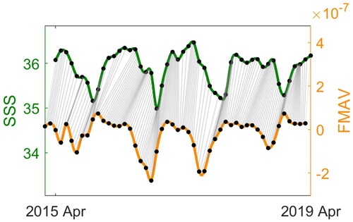
An analysis of such functional variables must, where possible, take into account the physical models that drive these processes. For instance, the underlying green and yellow curves in Figure 1(a) represent SSS and FMAV functions obtained by interpolating monthly-averaged data using cubic splines. (Throughout this work, the magnitude of SSS functions are in the practical salinity scale (pss) and the magnitude of FMAV functions is in pss/second.) Forcing, advection, and vertical mixing terms drive the dynamics of salinity in the upper ocean mixed layer (Bingham et al. 2010) via the SBE that reflects a simplified understanding of their relationship, (1) $$\frac{\partial S}{\partial t}=S_0\frac{E-P}{h}-\overrightarrow{u}·\nabla S-w\frac{\partial S}{\partial z},$$(1) where S is the mixed-layer salinity, t is time, S₀ is a constant given a canonical value of 35, and h is the mixed-layer depth. E represents evaporation, P precipitation, $\overrightarrow{u}$ the surface horizontal velocity, w the vertical velocity, and z is the vertical coordinate. The first term on the right-hand side is the surface freshwater forcing, the second is the horizontal advection, and the third is the vertical entrainment (this vertical mixing will be further decomposed into averaged and time-varying parts in Section 3.1).

Advection is the horizontal transport of salt. Entrainment is the vertical advection of salt or the mixing of salty or fresh water into the surface mixed layer. This process only operates when the vertical velocity is positive, ie in the upward direction. While the FMAV variable, which consists of the entire right-hand-side of Equation (1)(1) $$\frac{\partial S}{\partial t}=S_0\frac{E-P}{h}-\overrightarrow{u}·\nabla S-w\frac{\partial S}{\partial z},$$(1) , is known to drive the change of SSS on the left-hand side, unmodeled submesoscale motion or atmospheric processes near the upper ocean can affect the dynamics between SSS and FMAV, such that the two variables may appear to be out of phase. Moreover, it is feasible that perturbations from submesoscale processes in the upper ocean can give the appearance that SSS is leading FMAV for short periods of time. The goal of the present work is to study the phase relationship between SSS and FMAV. Understanding the differences in timing between these variables can help us understand how changes in the ocean are impacted by forcing through the salinity balance equation.

Due to the smooth variation of these variables, investigating their relationship requires the tools of functional data analysis. Statistical modeling of functional data must account for its underlying infinite-dimensional structure. Whereas one often assumes point-wise variation when working with multivariate data, the variation in functional data consists of two sources: phase and amplitude. The variation in the timing of important features of a functions, such as local extrema, is termed phase or $x-$ axis variability. Variation in the magnitude of measured values is called amplitude or $y-$ axis variability.

Estimated SSS and FMAV trajectories at a sample location at (10°N, 30°W) in the tropical North Atlantic Ocean are shown in Figure 1. Although we expect SSS and FMAV to evolve smoothly over time, we must work with monthly-averaged values (black markers) due to data availability, as detailed in Section 3.1. Cubic spline interpolation of the monthly-averaged data allows us to estimate their continuous trajectories (solid lines). The two functions clearly show similar shape features such as the number of peaks, which are not synchronized with one another. However, it is difficult to visually determine which of their differences are due to a lack of phase synchronization and which are due to differences in amplitude. The process of extracting these two confounded sources of variability is called registration (Ramsay and Li 1998), and is a relative procedure, in the sense that it is performed with respect to a chosen baseline function (typically one of the trajectories being analyzed). Thus, we say that one function has been registered to another.

In the case of the SSS and FMAV trajectories, registration would consist of alignment or the estimation of the relative phase between them that captures the timing difference of their common features. The resulting aligned functions, shown in Figure 1 may then be compared in terms of their amplitude. While the employed registration approach directly uses derivative information, we find it more intuitive to visualize the phase in the original state space, rather than the derivative space, which also enables comparison with results from a previous study (Bingham et al. 2012). One way to visualize continuous synchronization (via phase warping from function registration) of shape features between the two variables is to connect matched locations on the estimated functions with straight lines. A vertical line indicates perfect synchronization between the two functions at the connected locations, while a line with a positive (negative) slope indicates that FMAV is leading (trailing) SSS. We note that, as expected, the timing of features of the FMAV function for the most part precedes that of SSS, and the time lag varies across time. This varying phase difference may indicate the extent to which SSS variability is a seasonal process or is governed at some other time scale. More detailed results for this example are shown in the first row (Location 7) of Figure 4.

2. Functional Data with Phase Variation

Variability in the timing of importance features is a common feature of functional data. Such variability in timing is referred to as phase variability and the time-varying lag is represented by a phase function. In order to perform registration, one must first carefully define a distance metric over the function space of interest. This is critical, as estimating a phase function requires minimizing the distance between trajectories. Srivastava, Wu, et al. (2011) proposed using the extended Fisher-Rao (eFR) Riemannian metric, which satisfies some desirable properties such as invariance to warping, discussed below. This eFR metric-based registration method is referred to as elastic functional data analysis. The following subsections describe the elastic registration framework proposed by Srivastava, Wu, et al. (2011) as well as its properties.

2.1. Mathematical Framework

We assume that the functional data are absolutely continuous functions on the domain $[0,1],$ with the representation space $\mathcal{F}=\{f:[0,1]\to \mathbb{R}|f\text{ is absolutely continuous}\}.$ The domain can be easily generalized to any interval $[a,b]\subset \mathbb{R},a<b.$ This is reasonable in many applied problems, since the trajectories are assumed to evolve smoothly over time due to smooth phase warping and variation in amplitude, rather than the addition of point-wise noise. Observation error can also be included in a separate layer of the observation model on top of the functional data layer, or by pre-processing, as we have done in our analysis. A natural space of phase functions consists of orientation-preserving diffeomorphisms, (2) $$\Gamma =\{\gamma :[0,1]\to [0,1\left]\right|\gamma (0)=0,\gamma (1)=1,0<\dot{\gamma }<\infty \},$$(2) where $\dot{\gamma }$ is the time-derivative of function γ.

To achieve horizontal synchronization for two functions f₁ and f₂ in $\mathcal{F},$ we first select a reference function, say f₁, and find a phase element $\gamma \in \Gamma$ that best aligns the other function f₂ to the reference function through composition, $f_2°\gamma ,$ also called domain warping. The implied statistical model is that the reference function f₁ is a deformed version of f₂ through composition with an unknown phase function $\gamma \in \Gamma$ up to a discrepancy. We estimate the phase by finding an element in Γ that minimizes the discrepancy between these functions. One possible approach is to use the usual ${\mathbb{L}}^2$ norm between the reference function f₁ and the warped function f₂ as follows, (3) $$\widehat{\gamma }=\underset{{}_{\gamma \in \Gamma }}{\text{arginf}}\Vert f_1-(f_2°\gamma )\Vert ,$$(3) where $\left|\right|f\left|\right|$ denotes ${(\int |f(t){|}^{2}dt)}^{1/2}.$ However, there are some critical issues with using the ${\mathbb{L}}^2$ norm as a distance measure for function registration. One is that the solution is not symmetric, ie the minimum ${\mathbb{L}}^2$ norm for registration of f₁ to f₂ is not always the same as that for registration of f₂ to f₁, that is, $$\underset{\gamma \in \Gamma }{\inf }\parallel f_1-(f_2°\gamma )\left|\right|\ne \underset{\gamma \in \Gamma }{\inf }\left|\right|f_2-(f_1°\gamma )\left|\right|.$$

This notion of distance also fails to satisfy a key invariance property that is necessary for the registration of functions. For a distance metric $d(·),$ simultaneous domain warping is preserved when, $$d(f_1,f_2)=d(f_1°\gamma ,f_2°\gamma ),$$ for $f_1,f_2\in \mathcal{F}$ and any $\gamma \in \Gamma .$ Notably, the ${\mathbb{L}}^2$ distance does not satisfy this property, so another notion of distance must be considered.

The extended Fisher-Rao distance d_eFR proposed by Srivastava, Wu, et al. (2011) satisfies the key properties required for registration. Crucially, $d_{\mathit{eFR}}(f_1,f_2)=d_{\mathit{eFR}}(f_1°\gamma ,f_2°\gamma )$ for $f_1,f_2\in \mathcal{F}$ and any $\gamma \in \Gamma .$ However, the distance is not computable in closed form. To overcome this issue, Srivastava, Wu, et al. (2011) introduced a new representation of functions which makes the computation of the extended Fisher-Rao distance and the registration problem tractable. This square-root velocity function (SRVF) representation is given by the mapping $Q:\mathcal{F}\to \mathcal{Q}$ defined as, (4) $$Q(f)=\text{sign}(\dot{f})\sqrt{\left|\dot{f}\right|},f\in \mathcal{F},$$(4) where $\dot{f}$ is the time-derivative of f. The mapping Q is bijective up to the constant f(0), with inverse mapping $f(t)=Q^{-1}(f(0),q)(t)=f(0)+{\int }_0^{t}q(s)|q(s)|ds.$ Using this SRVF representation, the eFR metric simplifies to the standard ${\mathbb{L}}^2$ metric, ie $d_{\mathit{eFR}}(f_1,f_2)=d_{{\mathbb{L}}^2}(Q(f_1),Q(f_2))=\left|\right|Q(f_1)-Q(f_2)\left|\right|$ for $f_1,f_2,\in \mathcal{F}.$ Furthermore, the space of SRVFs $\mathcal{Q}$ is a subset of the function space ${\mathbb{L}}^2([0,1],\mathbb{R}).$

In the SRVF space, domain warping is achieved by the operation $(q,\gamma ):=(q°\gamma )\sqrt{\dot{\gamma }}$ where $q=Q(f)$ and it can be mapped back to the original function space via the inverse transformation $f(0)+{\int }_0^t(q,\gamma )(s)|(q,\gamma )(s)|ds=(f°\gamma )(t).$ The key distance property for function registration, invariance to simultaneous warping, can be proved as follows. For $q_1,q_2\in \mathcal{Q}$ and any $\gamma \in \Gamma ,$ (5) $$\begin{array}{c}{\Vert (q_1,\gamma )-(q_2,\gamma )\Vert }^2=\int {\left((q_1°\gamma )(t)\sqrt{\dot{\gamma }(t)}-(q_2°\gamma )(t)\sqrt{\dot{\gamma }(t)}\right)}^{2}dt,\\ =\int {\left(q_1(\gamma (t))-q_2(\gamma (t))\right)}^2\dot{\gamma }(t)dt,\\ =\int {\left(q_1(s)-q_2(s)\right)}^{2}ds=\left|\right|q_1-q_2|{|}^2,\end{array}$$(5) which is derived by substituting $\gamma (t)$ by s (Srivastava, Wu, et al. 2011). The amplitude of a function $f\in \mathcal{F}$ is defined as the equivalence class $[q]=\{(q,\gamma )|\gamma \in \Gamma \}$ where $q(=Q(f))\in \mathcal{Q}$ is its SRVF. The equivalence class is the set of SRVFs associated with all the phase components in the quotient space $\mathcal{Q}/\Gamma .$ The distance between two SRVFs $q_1,q_2\in \mathcal{Q}$ on the quotient space $\mathcal{Q}/\Gamma$ is defined as, (6) $$d\left(\left[q_1\right],\left[q_2\right]\right)=\underset{\gamma \in \Gamma }{\inf }\left|\right|q_1-(q_2,\gamma )\left|\right|.$$(6)

2.2. Phase Estimation

Having defined a suitable distance metric and exploiting the computational approach provided by the SRVF representation, we now turn to the problem of estimating a phase function by aligning two functions, also known as pairwise metric-based registration. Consider two functions $f_1,f_2\in \mathcal{F}$ that are related through domain warping as described above, with SRVFs $q_1,q_2\in \mathcal{Q}.$ We estimate the phase with $\gamma \in \Gamma$ that minimizes the ${\mathbb{L}}^2$ distance between q₁ and $(q_2,\gamma ),$ (7) $$\widehat{\gamma }=\arg \underset{{}_{\gamma \in \Gamma }}{\mathrm{min\hspace{0.17em}}}\left|\right|q_1-(q_2,\gamma )\left|\right|.$$(7)

The estimator can be computed efficiently using the dynamic programming (DP) algorithm introduced by Bertsekas (2000). The DP algorithm is a numerical algorithm that recursively searches for an optimal phase that minimizes the ${\mathbb{L}}^2$ distance between the SRVFs of two functions. The algorithm searches for an optimal phase by recursively finding a path on a 2-dimensional grid on the domain ${[0,1]}^2$ that minimizes the cost while using the cost of subpaths computed in the previous steps. Assuming that we want to find an optimal path reaching a point $(i/m,j/m)\in {[0,1]}^2,0<i,j\le m,$ denote a set of neighboring nodes below or left of the current point which can directly reach $(i/m,j/m)$ using a straight line by ${\mathcal{N}}_{(i,j)}.$ The cost of optimally reaching $(i/m,j/m)$ is (8) $$H_{i,j}=\underset{{}_{(k/m,l/m)\in {\mathcal{N}}_{i,j}}}{\min }\left(H_{k,l}+{\int }_{k/m}^{i/m}{\left(q_1(t)-q_2(\gamma (t))\sqrt{\dot{\gamma }(t)}\right)}^{2}dt\right).$$(8)

Since $H_{k,l},(k/m,l/m)\in {\mathcal{N}}_{i,j}$ has been computed while reaching the point $(i/m,j/m),$ we only need to compute the additional cost of each step.

Algorithm 1.

Phase Estimation Algorithm.

1: Let $H_{0,0}=0,H_{0,j/m}=\infty ,$ and $H_{i/m,0}=\infty$ for all $0<i,j\le m.$

2: for $(0,0)<(i/m,j/m)\le (1,1)$ do

3:   Compute $H_{i,j}$ using numerical integration.

4:   Denote $(k/m,l/m)$ that satisfies the minimization in $H_{i,j}$ by ${(\widehat{k}/m,\widehat{l}/m)}_{i,j}.$

5: end for

6: The algorithm below finds an optimal piecewise linear curve $\widehat{\gamma }.$

7: Let $(i/m,j/m)=(1,1).$

8: while $(i/m,j/m)\ne (0,0)$ do

9:   Let $(i/m,j/m)={(\widehat{k}/m,\widehat{l}/m)}_{i,j}$

10: end while

The results of this alignment procedure on the sample data in Figure 1 are shown in the first row (Location 7) of Figure 4. We choose SSS (green line in panel (a)) as the reference function and estimate the phase that best synchronizes FMAV (yellow line in panel (a)) to SSS. The aligned version of FMAV (yellow line) is plotted together with the original SSS variable (green line) in panel (c). The reference function SSS is unchanged from the original data in panel (a), while the aligned FMAV variable is obtained by composing SSS with the estimated phase. We observe that the local features of the two functions are well aligned. The relative phase between the SSS and FMAV functions is visualized in terms of the point-wise lag of FMAV with respect to SSS in panel (b) across time. A lag of 0 at a given time indicates that the two variables are perfectly synchronized at that time. A positive lag indicates that the dynamics of FMAV precede those of SSS, while a negative lag implies that FMAV trails SSS. While the timing of important shape features of FMAV mostly precedes that of SSS at this spatial location, it also trails that of SSS at certain times (eg around 2017 April). Interpretation of these results in the context of the dynamics of ocean salinity are provided in Section 4.

The general function registration procedure generates a phase that minimizes the distance between the input functions, warping the time domain to align one function to the other. While the estimated phase is dynamic over time, the procedure assumes that the two functions are fully aligned at the initial and the end points. This is because phase functions satisfy the boundary constraints $\gamma (0)=0$ and $\gamma (1)=1.$ However, in our case, there is an inherent lag between SSS and FMAV as seen in Equation (1)(1) $$\frac{\partial S}{\partial t}=S_0\frac{E-P}{h}-\overrightarrow{u}·\nabla S-w\frac{\partial S}{\partial z},$$(1) , where FMAV is related not to SSS itself, but to its time derivative. Thus, the assumption of endpoint synchronization may lead to a misleading result. To resolve this issue, we set the SSS function from April 2015 to April 2019 as a reference function and search for the domain of FMAV that minimizes the distance 6 from the SSS function. We try shifting the initial and end time points of FMAV a month (or two months) ahead of or after the initial and end time points of SSS and select the domain of FMAV that has the minimum distance between SSS and FMAV functions among the search grid. The results in Section 4 are derived using this procedure of searching for an optimal time domain for the FMAV function combined with functional registration.

3. Functional Data of SSS and FMAV

3.1. Data Sources

SSS and FMAV variables were constructed from a variety of sources. For SSS we used the Argo-based product of Roemmich and Gilson (2009). Evaporation comes from the OAflux product of Yu and Weller (2007) and Yu et al. (2008). The mixed layer depth we use is the MIMOC (Monthly Isopycnal & Mixed-layer Ocean Climatology) (Schmidtko et al. 2013). This is a climatology, so it does not provide values specific to a given month (eg January 2015), but rather average values for that month (ie January average). Precipitation is taken from the IMERG (Integrated Multi-satellitE Retrievals for GPM) precipitation product (Skofronick-Jackson et al. 2017). Surface velocity for computing horizontal advection is from the OSCAR (Ocean Surface Current Analysis Real-time) product (Bonjean and Lagerloef 2002). Near-surface vertical velocity was computed from Ekman convergence using the NOAA Coastwatch Ekman upwelling product. See Data Availability Statement for access information.

We interpolated, averaged, and subsampled to put all data on the same 1${}^{°}$ monthly grid from 63${}^{°}$S to 64${}^{°}$N and from October 2009 to September 2020. We calculated freshwater forcing (first term on the right-hand side of (1)) as in Equation (1)(1) $$\frac{\partial S}{\partial t}=S_0\frac{E-P}{h}-\overrightarrow{u}·\nabla S-w\frac{\partial S}{\partial z},$$(1) using the climatological mixed-layer depth.

We calculated horizontal advection as the dot product of surface velocity and the surface salinity gradient. The surface velocity product we used was already given in zonal and meridional components, and we calculated the zonal and meridional numerical partial derivatives of surface salinity from the monthly data.

We calculated vertical entrainment by combining the seasonal and average vertical velocity with the seasonal and average vertical salinity gradient, as given by (9) $$S\frac{\partial w}{\partial z}=w\prime \frac{\overline{\partial S}}{\partial z}+\overline{w}\frac{\partial S\prime }{\partial z}.$$(9)

We calculated vertical velocity by adding together Ekman upwelling and the vertical motion of the mixed-layer depth. Only water from below the mixed layer moving up changes the salinity of the water at the surface, so we set all downward vertical velocity values to zero. To calculate the vertical salinity gradient we used the difference between surface salinity and salinity 30 m below the average mixed layer depth, divided by the distance between them.

3.2. Data Pre-Processing

Monthly observations of SSS and FMAV are considered as realizations of an underlying smooth function. To explore the underlying smooth evolution of SSS and FMAV over time, we first apply cubic spline interpolation to the monthly SSS and FMAV values to evaluate SSS and FMAV functions over a fine temporal grid. Spline knots are placed at the temporal location where the monthly-averaged data is observed. The number of bases set to the number of knots plus 2 (ie order of the cubic spline minus 2).

An additional consideration is that the registration procedure must account for the different units of measurement between SSS and FMAV. As demonstrated in Section 2, SRVF representation used in the registration procedure is sensitive to differences in scales or units between functions. As shown on the left and right vertical axis of Figure 1 panel (a), the absolute values of FMAV are relatively much smaller than those of SSS. Thus, we first rescale the two functions by ensuring that the arc lengths equal 1 as presented by Srivastava, Klassen, et al. (2011), ie ${\int }_0^1|\dot{f}(t)|dt=1,$ which is equivalent to $\left|\right|q\left|\right|=1.$ When the original function is f and the rescaled function is $\tilde{f},$ rescaling is achieved via (10) $$\tilde{f}(t)=\frac{f(t)}{{\int }_0^1|\dot{f}(s)|ds},t\in [0,1].$$(10)

After estimating phase functions, we transform the rescaled functions to the original length for illustration purposes. The data and code to reproduce results presented in this work can be found at https://github.com/yoonj2kim/Seasonality-in-Sea-Surface-Salinity-Balance-Equation.

4. Comparing Temporal Dynamics of SSS and FMAV

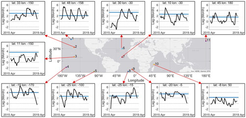
We estimate the relative phase between the SSS and FMAV functions at several locations (see map in Figure 2) from April 2015 to April 2019. Seasonality is clearly evident in many of the panels of Figure 2 and is the most important component of upper ocean salinity variability in many parts of the globe (Bingham and Lee 2017). This is probably driven by the seasonal cycle of rainfall and/or evaporation. As stated above, if the ocean were entirely seasonal, we would expect a 3-month lag between SSS and the forcing. However, that close relationship between SSS and seasonal forcing may break down at times. Other time scales are also important, eg the semi-annual especially at low latitudes (Yu et al. 2021) and El Niño (2–7 year) time scales. These kinds of processes may increase or decrease the phase lag relative to a strict seasonal cycle represented by harmonic analysis. Previous studies on evaluating seasonal variability of SSS and a combination of various terms of the upper ocean salinity balance equation have applied harmonic analysis to discrete observations and estimated the phase lag between SSS and FMAV by the difference in the times at which maximum SSS and FMAV are observed (Bingham et al. 2010, 2012, 2020; Boyer and Levitus 2002; Yu et al. 2021).

Figure 2. Visualization of 11 locations and estimated phase difference between SSS and FMAV at those locations. For each plot, the black function represents the phase estimated through the presented pairwise function registration procedure and the blue horizontal line shows the constant phase obtained via harmonic analysis for comparison. The black dashed lines serve as reference.

We explore how the dynamics of the component terms of SBE, the original series of SSS and FMAV, vary together and whether there are any deviations from the established theoretical understanding of the causal relationship between the two components. While the SBE in Equation (1)(1) $$\frac{\partial S}{\partial t}=S_0\frac{E-P}{h}-\overrightarrow{u}·\nabla S-w\frac{\partial S}{\partial z},$$(1) represents a simplified theoretical understanding of their relationship, the realities of the ocean might be different. For our analysis, we restricted attention to locations in the ocean where there was evidence of both a constant and a continuous warping between SSS and FMAV, that is where the two variables had statistically significant harmonic fit as described by Bingham et al. (2012) and where SSS and FMAV have small distance after performing elastic function registration. We estimated phase functions from these 21 locations and compared them to phase differences obtained via harmonic analysis. For visualization, we selected 11 among these 21 locations that were as spatially spread out as possible to convey the spatial pattern most informatively with the fewest plots, since data from adjacent locations suggests very similar dynamics.

Figure 2 displays the 11 locations and the functions representing time lag between SSS and FMAV at those locations. We first estimate phase functions ${\widehat{\gamma }}_i,i=1,\dots ,11,$ and derive the estimated time lag ${\widehat{l}}_i$ by transforming the phase ${\widehat{\gamma }}_i$ via (11) $${\widehat{l}}_i={\widehat{\gamma }}_i-{\gamma }_{id},$$(11) where γ_id is the identity phase function. If the initial and end points of SSS and FMAV are the same, then ${\gamma }_{id}(t)=t,\forall t.$ However, if the starting and ending points for FMAV are shifted, the domain of γ_id is shifted accordingly, whereas the $y-$ values are preserved. The black curves represent the estimated time lag between the FMAV and SSS functions across time. The estimated lags tend to fluctuate to as much as six months. On the seasonal scale, Delcroix et al. (1996) expect a three-month lag between FMAV and SSS with FMAV leading. However, the estimated lag functions show that the phase difference between SSS and FMAV may vary both across time and location. The blue horizontal line shows the phase differences using simple harmonic analysis on the monthly observations of the two variables. For most of the locations, the average of the estimated lags across time tends be close to the phase difference obtained via harmonic analysis. However, there are locations where the estimated lag functions are far from the constant estimate of phase difference, eg locations 3 and 10.

Figures 3 and 4 show the SSS and FMAV functions of the 11 locations from Figure 2 and their lag functions, estimated using the functional registration procedure. For each location, column (a) shows the SSS and FMAV trajectories in green and yellow, respectively. The gray lines represent the matching of SSS and FMAV achieved by the domain warping across time that minimizes the distance between the two functions. Note that an interval of one variable may be synchronized to a shorter or longer interval of the other variable. For example, for Location 7, a short interval near the deepest valley of SSS is connected to a longer interval near the deepest valley of FMAV, and the resulting alignment of those intervals of FMAV to SSS is achieved by squeezing in the longer interval of SSS to the short interval of FMAV. Such nonlinear shift of FMAV across the domain results in better matching of features of SSS and FMAV.

Figure 3. Summary of estimated lag functions from function registration and phases from harmonic analysis at location 1 through 6. The index of locations as indicated in Figure 2 is in the first column. Column (a) displays the SSS (in green) and FMAV (in yellow) functions of each location. The gray lines represent the matching of SSS and FMAV achieved by function registration. In column (b) are the lag functions derived using the function registration in black (in the same manner as Figure 1(b)) and the time lag estimated by harmonic analysis in blue. The resulting alignment of functions are displayed in column (c) using the same colors.

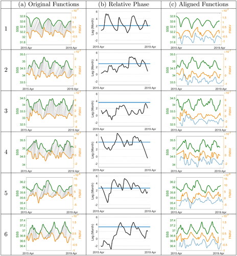
Figure 4. Continued summary of estimated lag functions from function registration and phases from harmonic analysis at location 7 through 11 in the same manner as Figure 3. (a) The SSS (in green) and FMAV (in yellow) functions of each location with the gray lines representing the matching of SSS and FMAV achieved by function registration. (b) The lag functions derived using the function registration in black and the time lag estimated by harmonic analysis in blue. (c) The resulting alignment of functions.

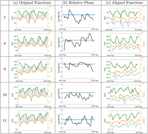
Column (b) shows the lag functions between SSS and FMAV estimated by function registration in black and the phase difference estimated through harmonic analysis as a blue horizontal line - the same curves as in 2. In column (c), the green curve is the SSS function in (a) and the yellow curve is the result of the registration of FMAV to SSS achieved by applying the estimated lag function (black) in panel (b) to the FMAV trajectory. The blue curve in panel (c) is the FMAV function shifted by the constant phase difference estimated using harmonic analysis, which is illustrated by the blue horizontal line in panel (b). Examining the registration results in panel (c), the presented function registration approach appears to be more effective in synchronizing the two functions in time.

While the phase difference presented by Bingham et al. (2012) aims to estimate a global phase difference with a constant value, it may not capture local phase variability which may change across time. For example, for location 2, the local extremes of the yellow function are well aligned to the SSS function. However, not all the local extremes of the blue function are horizontally synchronized to the green function. For locations 3 and 10, the estimated lag functions are far from the time lag estimated from harmonic analysis. Locations 3 and 10 are places in the ocean with especially strong seasonal variability (see eg (Yu et al. 2021, Figures 5 and 9)). Location 3 is in the eastern tropical Pacific at the very northward edge of the influence of the seasonal migration of the intertropical convergence zone. This is a very dynamic region, impacted by eddy transport Hasson et al. (2018, 2019), tropical instability waves, and El Niño. Location 10 in the western South Indian Ocean just north of Madagascar is close to the equator and impacted by small-scale Ekman transport that may not be well-represented in the monthly products used to formulate the FMAV for this study (Yu 2011). In these locations, the seasonal cycle of SSS might be prominent but not governed as much by the terms on the right-hand side of Equation (1)(1) $$\frac{\partial S}{\partial t}=S_0\frac{E-P}{h}-\overrightarrow{u}·\nabla S-w\frac{\partial S}{\partial z},$$(1) .

The registration of these locations shows that the presented approach is more effective in estimating local phase variability and horizontally synchronizing the important features of the two variables. As expected, we see FMAV leading SSS across most of the time domain at all the locations. Occasional periods where FMAV appears to trail SSS may be due to so-called submesoscale motion in the ocean that can have an impact on mixed-layer properties while having no immediate connection to the forcing function we have computed. The relatively short duration of these periods and their occurrence near the endpoints of the domain or after a large change in phase also suggest the possibility that they may be due to an artefact of model fitting or pre-processing. In either case, this fact motivates further analysis.

Table 1 reports (A) the distance between SSS and FMAV registered to SSS and (B) the distance between SSS and FMAV shifted by the constant phase difference estimated using harmonic analysis at the 11 locations under consideration. Both distances are computed in the SRVF space to measure the difference in shapes (or fluctuation) of SSS and FMAV and to quantify the performance of two different alignment results. Let ${\widehat{h}}_i,i=1,\dots ,11$ be the constant phase difference obtained using the harmonic analysis of location i and denote the SRVFs of SSS and FMAV at location i by s_i and f_i, respectively. Then distance A is calculated as $({\int }_{l{b}_i}^{u{b}_i}(s_i(t)-f_i({\widehat{\gamma }}_i(t)){)}^{2}dt{)}^{-1/2}$ and distance B is $({\int }_{l{b}_i}^{u{b}_i}(s_i(t)-f_i(t+{\widehat{h}}_i){)}^{2}dt{)}^{-1/2}$ where the lower and upper bounds of the time domain lb_i and ub_i are determined by the overlapping time domain of SSS (green), FMAV optimally aligned to SSS using function registration (yellow), and FMAV shifted using harmonic analysis (blue). Distance B was approximately twice the magnitude of distance A across locations, suggesting that function registration better aligns SSS and FMAV compared to alignment with a constant phase (harmonic analysis). While not presented in this work, analyses of other locations across the ocean showed that the function registration method aligns the timing of important features well and yields a smaller registered distance compared to the harmonic analysis method.

Table 1. (A) Distance between SSS function and FMAV function registered to SSS achieved by applying the estimated lag function; (B) Distance between SSS function and FMAV function shifted by the constant phase difference estimated using harmonic analysis.

Location	1	2	3	4	5	6
A	0.6221	0.6020	0.6928	0.5329	0.6885	0.5226
B	1.3552	1.3596	1.2720	1.0593	1.3171	1.2535
Location	7	8	9	10	11
A	0.5436	0.7620	0.5067	0.8359	0.5975
B	1.2362	1.2241	1.2964	1.2209	1.1540

5. Discussion and Conclusions

Our analysis is an exploration of ocean processes that manifest as time shifts between SSS and FMAV, the two components of the SBE. We have applied the tools of elastic functional data analysis to the problem of investigating the dynamic time lag between these variables at a variety of locations in the global ocean (Figure 2). We found that estimating phase as a dynamic variable is more effective in explaining local phase variability compared to the more traditional approach of constant phase estimation via harmonic analysis. A major advantage to our method is that relative phase can be allowed to vary over time, whereas harmonic analysis provides one value of phase for an entire dataset. In the case of SSS, seasonal processes are often the most important (Bingham and Lee 2017), but the relative phase can vary from the expected 1/4 cycle due to internal ocean dynamics like vertical entrainment (Figures 3 and 4).

The results are based on some simplifying assumptions, which may not reflect the true state of the ocean. For instance, our model does not account for the possible presence of serially-correlated errors and the effect of omitted variables related to submesoscale motion. Including these components into the analysis would require using a model-based approach to elastic registration, such as that presented in Matuk et al. (2021), which treats the registration step as a layer within a Bayesian hierarchical model.

The analysis demonstrates how the phase difference between SSS and FMAV can be estimated, but it does not indicate how the SSS phase may be related to the individual components of FMAV. The work of (Bingham et al. 2012) shows that surface freshwater forcing has a seasonal phase that is 1–2 months ahead of where it would be predicted based on SSS alone through the upper ocean salinity balance equation. In other words, horizontal advection and vertical entrainment act to delay the ocean’s response to atmospheric forcing. A simple extension of this work would be to apply it on a more global basis and use it to explore this phase delay, how it varies, and how it relates to the mix of processes that impact the upper ocean in different amounts at different locations. The ultimate goal of studying the phase offset (and SSS in general) is to understand the role of SSS as an indicator or an active participant in the global water cycle (Durack 2015), and being able to sort out the phase contributions of the various processes that act to change SSS can help us do that.

Disclosure Statement

No potential conflict of interest was reported by the author(s).

Data Availability Statement

Data used in this paper come from the following sources:

• Roemmich & Gilson SSS: https://sio-argo.ucsd.edu/RG/_Climatology.html.

• OAFlux evaporation: https://climatedataguide.ucar.edu/climate-data/oaflux-objectively-analyzed-air-sea-fluxes-global-oceans.

• MIMOC mixed layer depth: https://www.pmel.noaa.gov/mimoc/.

• GPM IMERG precipitation: https://gpm.nasa.gov/data/imerg.

• OSCAR surface velocity: https://podaac.jpl.nasa.gov/dataset/OSCAR/_L4/_OC/_third-deg.

• NOAA Coastwatch Ekman Upwelling: https://coastwatch.pfeg.noaa.gov/erddap/griddap/erdQAstressmday.html.

Additional information

Funding

This work was funded as part of NASA’s Ocean Salinity Science Team under NASA Grant No. [80NSSC18K1322].

References

- Bertsekas DP. 2000. Dynamic programming and optimal control. 2nd ed. Belmont (MA): Athena Scientific.
- Bingham FM, Brodnitz S, Yu L. 2020. Sea surface salinity seasonal variability in the tropics from satellites, gridded in situ products and mooring observations. Remote Sensing. 13(1):110.
- Bingham FM, Foltz GR, McPhaden MJ. 2010. Seasonal cycles of surface layer salinity in the Pacific ocean. Ocean Sci. 6(3):775–787.
- Bingham FM, Foltz GR, McPhaden MJ. 2012. Characteristics of the seasonal cycle of surface layer salinity in the global ocean. Ocean Sci. 8(5):915–929.
- Bingham FM, Lee T. 2017. Space and time scales of sea surface salinity and freshwater forcing variability in the global ocean (60°S–60°N). JGR Oceans. 122(4):2909–2922.
- Bonjean F, Lagerloef GS. 2002. Diagnostic model and analysis of the surface currents in the tropical Pacific ocean. J Phys Oceanogr. 32(10):2938–2954.
- Boyer TP, Levitus S. 2002. Harmonic analysis of climatological sea surface salinity. J Geophys Res. 107(C12):SRF 7-1–SRF 7-14.
- Delcroix T, Henin C, Porte V, Arkin P. 1996. Precipitation and sea-surface salinity in the tropical pacific ocean. Deep Sea Res Part I. 43(7):1123–1141.
- Durack PJ. 2015. Ocean salinity and the global water cycle. oceanog. 28(1):20–31.
- Hasson A, Farrar JT, Boutin J, Bingham F, Lee T. 2019. Intraseasonal variability of surface salinity in the eastern tropical pacific associated with mesoscale eddies. JGR Oceans. 124(4):2861–2875.
- Hasson A, Puy M, Boutin J, Guilyardi E, Morrow R. 2018. Northward pathway across the tropical North Pacific Ocean revealed by surface salinity: how do El Niño anomalies reach Hawaii? J Geophys Res Oceans. 123(4):2697–2715.
- Matuk J, Bharath K, Chkrebtii O, Kurtek S. 2021. Bayesian framework for simultaneous registration and estimation of noisy, sparse, and fragmented functional data. J Am Stat Assoc. 117(540):1–34.
- Ramsay J, Li X. 1998. Curve registration. J R Stat Soc B. 60(2):351–363.
- Ramsay J, Silverman BW. 2005. Functional data analysis. New York: Springer.
- Roemmich D, Gilson J. 2009. The 2004–2008 mean and annual cycle of temperature, salinity, and steric height in the global ocean from the Argo Program. Prog Oceanogr. 82(2):81–100.
- Schmidtko S, Johnson GC, Lyman JM. 2013. Mimoc: a global monthly isopycnal upper-ocean climatology with mixed layers. J Geophys Res Oceans. 118(4):1658–1672.
- Skofronick-Jackson G, Petersen WA, Berg W, Kidd C, Stocker EF, Kirschbaum DB, Kakar R, Braun SA, Huffman GJ, Iguchi T, et al. 2017. The global precipitation measurement (GPM) mission for science and society. Bull Am Meteorol Soc. 98(8):1679–1695.
- Srivastava A, Klassen E, Joshi SH, Jermyn IH. 2011. Shape analysis of elastic curves in Euclidean spaces. IEEE Trans Pattern Anal Mach Intell. 33(7):1415–1428.
- Srivastava A, Wu W, Kurtek S, Klassen E, Marron JS. 2011. Registration of functional data using Fisher-Rao metric. arXiv.
- Vinogradova N, Lee T, Boutin J, Drushka K, Fournier S, Sabia R, Stammer D, Bayler E, Reul N, Gordon A, et al. 2019. Satellite salinity observing system: recent discoveries and the way forward. Front Mar Sci. 6:243.
- Yu L. 2011. A global relationship between the ocean water cycle and near-surface salinity. J Geophys Res. 116(C10):10025.
- Yu L, Bingham FM, Lee T, Dinnat EP, Fournier S, Melnichenko O, Tang W, Yueh SH. 2021. Revisiting the global patterns of seasonal cycle in sea surface salinity. JGR Oceans. 126(4):e2020JC016789.
- Yu L, Jin X, Weller RA. 2008. Multidecade global flux datasets from the objectively analyzed air-sea fluxes (oaflux) project: latent and sensible heat fluxes, ocean evaporation, and related surface meteorological variables. Woods Hole: Woods Hole Oceanographic Institution. OAFlux Project Technical Report OA-2008-01.
- Yu L, Weller RA. 2007. Objectively analyzed air–sea heat fluxes for the global ice-free oceans (1981–2005). Bull Am Meteorol Soc. 88(4):527–540.