Mixture of Regressions with Multivariate Responses for Discovering Subtypes in Alzheimer’s Biomarkers with Detection Limits

Abstract

There is no gold standard for the diagnosis of Alzheimer’s disease (AD), except for autopsies, which motivates the use of unsupervised learning. A mixture of regressions is an unsupervised method that can simultaneously identify clusters from multiple biomarkers while learning within-cluster demographic effects. Cerebrospinal fluid (CSF) biomarkers for AD have detection limits, which create additional challenges. We apply a mixture of regressions with a multivariate truncated Gaussian distribution (also called a censored multivariate Gaussian mixture of regressions or a mixture of multivariate Tobit regressions) to over 3000 participants from the Emory Goizueta Alzheimer’s Disease Research Center and Emory Healthy Brain Study to examine amyloid-beta peptide 1–42 (Abeta42), total tau protein and phosphorylated tau protein in CSF with known detection limits. We address three gaps in the literature on the mixture of regressions with a truncated multivariate Gaussian distribution: software availability; inference; and clustering accuracy. We discovered three clusters that tend to align with an AD group, a normal control profile, and non-AD pathology. The CSF profiles differed by race, gender, and the genetic marker ApoE4, highlighting the importance of considering demographic factors in unsupervised learning with detection limits. Notably, African American participants in the AD-like group had significantly lower tau burden.

Keywords:

• Alzheimer’s disease
• censored Gaussian mixture of regressions
• clustering
• finite mixture model
• latent class analysis
• Tobit model
• truncated normal
• unsupervised learning

1. Introduction

A definitive diagnosis of Alzheimer’s disease (AD) is only possible from an examination of brain tissue in an autopsy (Dubois et al. 2007). The clinical diagnosis of AD typically involves a combination of cognitive assessments, physical exams, neurological exams, and medical history evaluation (McKhann et al. 1984). Updated criteria incorporate positron emission tomography (PET) and cerebrospinal fluid (CSF) biomarkers to support the diagnosis, including cut-offs based on amyloid beta, total tau, and phosphorylated tau (McKhann et al. 2011). A biomarker cut-off classifies a patient with a disease if their biomarker level exceeds a threshold. CSF and imaging biomarker cut-offs are imperfect due to uncertainty in the diagnostic labels used to determine them. The problem is made worse by the fact that clinical diagnosis using biomarkers has historically been based on studies dominated by people of European ancestry (Blennow et al. 2015). African American individuals are greatly underrepresented in AD biomarker studies and clinical trials (Shin and Doraiswamy 2016), and CSF biomarker levels differ by race (Garrett et al. 2019). There are at least three challenges to analyzing CSF AD biomarker data: (1) multivariate biomarkers have detection limits, i.e. biomarker values exceed a value that can be measured by the assay, which results in censoring; (2) the disease status is unknown since there is no gold standard; and (3) demographic effects may depend on unknown subtypes. Current statistical software does not simultaneously address these problems (Table 1).

Table 1. List of finite mixture modeling software.

Packages	Censored outcomes	Multivariate outcomes	Mixture of regressions	Truncated multivariate normal
mclust	✗	✓	✗	✗
mixtools	✗	✓	✓	✗
FlexMix	✗	✗	✓	✗
SMNCensReg	✓	✗	✗	✗
CensMFM	✓	✓	✗	✗
poLCA	✗	✗	✓	✗
CensMixReg	✓	✗	✓	✗
fmm (Stata)	✓	✗	✓	✗
proc fmm (SAS)	✓	✗	✓	✗
Latent GOLD 6.0	✓	✓	✓	✗

mclust: Scrucca et al. (2016); mixtools: Benaglia et al. (2009); FlexMix: Leisch (2004); SMNCensReg: Garay et al. (2013); CensMFM: De Alencar et al. (2020); poLCA: Linzer and Lewis (2011); CensMixReg: Sanchez et al. (2018); Latent GOLD 6.0: Vermunt and Magidson (2021).

We analyze a dataset from the Emory Goizueta Alzheimer’s Disease Research Center and the Emory Healthy Brain Study (hereafter, Emory ADRC/HBS Dataset), which contains three CSF biomarkers (amyloid-beta peptide 1–42 [Abeta42], total tau protein [tTau] and phosphorylated tau protein [pTau]) from lumbar punctures of over $3,\mathrm{}000$ individuals (Goetz et al. 2019). The dataset contains 16.5% (495) African American participants, which is substantially higher than the Alzheimer’s Disease Neuroimaging Initiative ($<5\%$). An important limitation of the assay is that ∼15% of the participants in the Emory ADRC/HBS dataset have one of the three biomarker levels defined by the detection limits of the assay. In this paper, we define a censored response variable in the same way as other mixture modeling papers (Jedidi et al. 1993; Lee and Scott 2012): censoring occurs if the value of the response variable is set equal to the detection limit when the true value is more extreme than the threshold, while the predictors are available for all observations (e.g. participants with Abeta42 over 1700 have their Abeta42 values set equal to 1700). This differs from truncation, which typically refers to a restricted sampling of the distribution of the population (e.g. if patients with Abeta42 over 1700 were not recorded, then the data would be truncated).

Unsupervised learning, such as Gaussian mixture models (GMMs), are popular tools for defining disease subtypes when a gold standard is not available (Collins and Huynh 2014). GMMs were applied to CSF biomarkers to identify patterns in AD without the use of diagnosis (Meyer et al. 2010). Model-based clustering approaches derived from GMMs have advantages over distance-based clustering algorithms, such as K-means. GMMs estimate posterior probabilities of group membership for each data point rather than hard clustering. GMMs utilize a statistical model that can account for correlations. From a probabilistic perspective, K-means assumes spherically shaped clusters, which can lead to poor results when features are correlated (Coates and Ng 2012). In our application, CSF biomarkers of AD are highly correlated. A Gaussian mixture of regressions (GMR) model, also called “switching regressions” in econometrics, extends GMMs to datasets with predictors by modeling the mean structure of each group using regression (Goldfeld and Quandt 1973; Quandt and Ramsey 1978). These models allow for the effect of predictors to be modified by the latent groups. These models have also been extensively discussed in the machine learning literature, where they are called “mixture of experts” models (Yuksel et al. 2012).

Censored multivariate Gaussian mixtures of regressions (censored GMRs), also known as a mixture of regressions with a truncated multivariate Gaussian distribution or a multivariate mixture of Tobit regressions, have been previously considered in the literature. Lee and Scott (2012) derived EM algorithms for fitting multivariate GMMs to censored data. To model predictors, Jedidi et al. (1993) derived an EM algorithm for a mixture of Tobit regressions with a univariate censored response, and more recent extensions of Tobit regression for a univariate response model errors using a finite mixture of Gaussian and/or non-Gaussian distributions (Caudill 2012; Garay et al. 2017; Hanson and Johnson 2002; Karlsson and Laitila 2014; Zeller et al. 2019). Wang et al. (2019) proposed a mixture of factor analyzers for multivariate data that simultaneously performs clustering and dimension reduction, and Wang et al. (2021) extended it to predictors and censoring.

Our goals are 2-fold: (1) cluster participants into groups using an unsupervised multivariate method, since no gold standard is available and current criteria may be limited by factors, such as European ancestry, and (2) gain insights into pathophysiology by estimating within-cluster effects of demographic variables (race, gender, the genetic marker ApoE4, age, and education). Our primary contribution is an analysis of the Emory ADRC/HBS dataset using a censored multivariate Gaussian mixture of regressions. We implement an EM algorithm to address the important gap that software does not exist for the censored multivariate Gaussian mixture of regressions. We also address gaps in the current literature regarding the use of Wald tests of significance of the predictors in this context, wherein we approximate the information matrix using the empirical complete data score function. We also conduct a simulation study to address a gap regarding the impact of predictors and censoring on the accuracy of clustering.

The remainder of this paper is organized as follows. In Section 2, we review the multivariate Tobit model and describe the extension to censored Gaussian mixtures. We then describe an EM algorithm and method for inference. In Section 3, we conduct simulations to illustrate the advantages of the censored multivariate GMR over methods ignoring or deleting the censored observations, and we also examine the selection of the number of clusters. In Section 4, we conduct an analysis of the Emory ADRC/HBS Dataset. Finally, we discuss findings and future research in Section 5.

2. Modeling Approach and Estimation

In this section, we first review the multivariate Tobit model and its estimation using an expectation-maximization (EM) algorithm. We then build upon this framework to derive an EM algorithm for the censored multivariate GMR.

2.1. Multivariate Censored Regression (Tobit Model)

Let ${\mathbf{y}}_i$ be a p-dimensional random vector denoting the observed biomarkers (for example, in this study, the CSF biomarkers: amyloid-beta peptide 1–42 [Abeta42], total tau protein [tTau] and phosphorylated43 tau protein [pTau]) for the ith subject, $i=1,\dots ,N,$ which can be partitioned into two parts, $${\mathbf{y}}_i=\left(\begin{array}{c}{\mathbf{y}}_{i{o}_i}\\ {\mathbf{y}}_{i{c}_i}\end{array}\right),i\in \{1,2,\dots ,N\},$$ where ${\mathbf{y}}_{i{o}_i}$ and ${\mathbf{y}}_{i{c}_i}$ denote the uncensored and censored dimensions of ${\mathbf{y}}_i$ (for example, in this study, the fully observed biomarkers and the biomarkers that are censored due to detection limits). We use a vector of censoring indicators ${\mathit{c}}_i$ to represent whether or not one particular dimension of ${\mathbf{y}}_i$ is censored, and its censoring directions are observed through ${\mathit{c}}_i={(c_{i1},\dots ,c_{\mathit{\text{ij}}},\dots ,c_{\mathit{\text{ip}}})}^{\top },$ where ${}^{\top }$ denotes the transpose, such that: $$c_{\mathit{\text{ij}}}=\{\begin{array}{cc}1,\hfill & \text{Right‐censored},\hfill \\ 0,\hfill & \text{Uncensored},\hfill \\ -1,\hfill & \text{Left‐censored}.\hfill \end{array}$$

Though the true values are not observed before they are censored, we can nevertheless further assume ${\mathbf{y}}_i$ are generated from the partially unobserved truth, as a latent random vector ${\mathbf{y}}_i^{*}={(y_{i1}^{*},\dots ,y_{\mathit{\text{ij}}}^{*},\dots ,y_{\mathit{\text{ip}}}^{*})}^{\top }$ with some known lower and upper detection limits: $$y_{\mathit{\text{ij}}}=\{\begin{array}{c}{L}_j\mathrm{\hspace{1em}}\mathrm{\hspace{1em}}\text{if}\mathrm{\hspace{1em}}\mathrm{\hspace{1em}}{y}_{\mathit{\text{ij}}}^{*}\le L_j,\hfill \\ y_{\mathit{\text{ij}}}^{*}\mathrm{\hspace{1em}}\mathrm{\hspace{1em}}\text{if}\mathrm{\hspace{1em}}\mathrm{\hspace{1em}}{L}_j<y_{\mathit{\text{ij}}}^{*}<U_j,\hfill \\ U_j\mathrm{\hspace{1em}}\mathrm{\hspace{1em}}\text{if}\mathrm{\hspace{1em}}\mathrm{\hspace{1em}}{y}_{\mathit{\text{ij}}}^{*}\ge U_j.\hfill \end{array}$$

Similarly, we can partition ${\mathbf{y}}_i^{*}$ into observed and censored parts: $${\mathbf{y}}_i^{*}=\left(\begin{array}{c}{\mathbf{y}}_{i{o}_i}\\ {\mathbf{y}}_{i{c}_i}^{*}\end{array}\right),i\in \{1,2,\dots ,N\},$$ where ${\mathbf{y}}_{i{c}_i}^{*}$ are unobserved and censored as ${\mathbf{y}}_{i{c}_i}.$ In a multivariate regression model setting, we also assume ${\mathit{x}}_i$ is a d-dimensional vector that represents the observed predictors of the ith subject (for example, in this study, patients’ age, education, gender, and APOE4 genotypes). Then, the model can be formed as (1) $${\mathbf{y}}_i^{*}={\mathit{\beta }}^{\top }{\mathit{x}}_i+{\mathit{ϵ}}_i,$$(1) where $\mathit{\beta }$ is a d × p coefficient matrix and a primary parameter of interest (for example, in this study, the effects of patients’ age, education, gender, and APOE4 genotypes on the CSF biomarkers), ${\mathit{ϵ}}_i$ is a p-dimensional vector of random noise and ${\mathit{ϵ}}_i\stackrel{i.i.d.}{\sim }\mathcal{N}(\mathbf{0},\mathbf{\Sigma }).$

Let $\mathit{\psi }$ denote the collection of parameters $\mathit{\beta }$ and $\mathbf{\Sigma }.$ Let Y be the N × p matrix of stacked observations ${\mathbf{y}}_i^{\top },$ C be the N × p matrix of stacked censoring directions ${\mathit{c}}_i^{\top };$ and X the N × d matrix of stacked predictor vectors ${\mathit{x}}_i^{\top }.$ Then $\mathit{\psi }$ can be estimated from maximization of the incomplete data likelihood function: (2) $$\mathcal{L}(\mathbf{Y};\mathbf{C},\mathbf{X},\mathit{\psi })=\prod _{i=1}^N{f}_{{\mathbf{y}}_{i{o}_i}}({\mathbf{y}}_{i{o}_i};{\mathit{x}}_i,\mathit{\psi }){\int }_{\mathcal{D}({\mathit{c}}_i)}{f}_{{\mathbf{y}}_{i{c}_i}^{*}|{\mathbf{y}}_{i{o}_i}}({\mathbf{y}}_{i{c}_i};{\mathit{x}}_i,\mathit{\psi }),$$(2) where $\mathcal{D}({\mathit{c}}_i)$ is a domain in ${\mathbb{R}}^p,$ depending on the censored patterns represented by ${\mathit{c}}_i,$ and $f_{{\mathbf{y}}_{i{c}_i}^{*}|{\mathbf{y}}_{i{o}_i}}$ is the conditional Gaussian density of the unobserved responses ${\mathbf{y}}_{i{c}_i}^{*}$ that experience censoring given the observed responses without censoring ${\mathbf{y}}_{i{o}_i}.$ Typically, (2) is maximized numerically by the Newton–Raphson method (Amemiya 1973). Here, we outline the EM algorithm similar to Fair (1977; Ruud 1991), which we will extend to Gaussian mixtures in Section 2.2. Let ${\mathbf{Y}}^{*}$ denote the N × p matrix of true observations formed by stacking ${\mathbf{y}}_i^{*\top }.$ Define the complete data likelihood assuming ${\mathbf{y}}_i^{*},i=1,\dots ,N,$ are observed: $${\mathcal{L}}_c({\mathbf{Y}}^{*};\mathbf{C},\mathbf{X},\mathit{\psi })=\prod _{i=1}^N\frac{1}{\sqrt{2^p{\pi }^p\left|\mathbf{\Sigma }\right|}}{e}^{-\frac{1}{2}{({\mathbf{y}}_i^{*}-{\mathit{\beta }}^{\top }{\mathit{x}}_i)}^{\top }{\mathbf{\Sigma }}^{-1}({\mathbf{y}}_i^{*}-{\mathit{\beta }}^{\top }{\mathit{x}}_i)}.$$

The EM algorithm steps are derived by maximization of the conditional expectation of this complete data log-likelihood function, with details in Web Supplement 1.1.

2.2. Censored Multivariate Gaussian Mixture of Regressions

The multivariate censored regression in Section 2.1 assumes no underlying subgroups and the effects of the predictors are homogeneous. In this study, we suspect there are subgroups in which coefficients of demographic predictors differ. Therefore, we use the censored multivariate GMR model.

Let G denote the number of clusters (e.g. in this study, disease subgroups). Later, we examine the selection of G using information criteria. Then we can expand the model in (1) to a mixture model: $${\mathbf{y}}_i^{*}|g={\mathit{\beta }}_g^{\top }{\mathit{x}}_i+{\mathit{ϵ}}_{\mathit{\text{ig}}},g\in \{1,..,G\}.$$

Therefore, ${\mathbf{y}}_i^{*}\left|\right\{g,{\mathit{x}}_i\}\sim \mathcal{N}({\mathit{\beta }}_g^{\top }{\mathit{x}}_i,{\mathbf{\Sigma }}_g).$ Assuming observations are i.i.d., define the incomplete data likelihood function: $$\mathcal{L}(\mathbf{Y};\mathbf{C},\mathbf{X},\mathbf{\Psi })=\prod _{i=1}^N\sum _{g=1}^G{\omega }_g{f}_{{\mathbf{y}}_{i{o}_i}}({\mathbf{y}}_{i{o}_i};{\mathit{x}}_i,{\mathit{\psi }}_g){\int }_{\mathcal{D}({\mathit{c}}_i)}{f}_{{\mathbf{y}}_{i{c}_i}^{*}|{\mathbf{y}}_{i{o}_i}}({\mathbf{y}}_{i{c}_i};{\mathit{x}}_i,{\mathit{\psi }}_g),$$ where ${\mathit{\psi }}_g$ are the vectorized parameters for each component; ${\omega }_g\in (0,1)$ are the mixing proportions of each mixture component subject to constraint: ${\sum }_{g=1}^G{\omega }_g=1;$ and $\mathbf{\Psi }$ is the overall parameter vector, such that $\mathbf{\Psi }=({\omega }_1,\dots ,{\omega }_{G-1},{\mathit{\psi }}_1,\dots ,{\mathit{\psi }}_G).$ Unlike the previously described regression model, in a mixture model setting, the direct maximization of the above likelihood function is not possible. Thus, we utilize the EM algorithm for parameter estimation. Let z_ig denote an indicator variable equal to one if the ith subject is in the gth group and zero otherwise, and let Z denote the N × G matrix formed by stacking ${[z_{i1},\dots ,z_{\mathit{\text{iG}}}]}^{\top }.$ Assuming both Z and ${\mathbf{Y}}^{*}$ are observed, we can write the complete data likelihood function: $${\mathcal{L}}_c({\mathbf{Y}}^{*},\mathbf{Z};\mathbf{C},\mathbf{X},\mathbf{\Psi })=\prod _{i=1}^N\prod _{g=1}^G{\left\{\frac{{\omega }_g}{\sqrt{2^p{\pi }^p\left|{\mathbf{\Sigma }}_g\right|}}{e}^{-\frac{1}{2}{({\mathbf{y}}_i^{*}-{\mathit{\beta }}_g^{\top }{\mathit{x}}_i)}^{\top }{\mathbf{\Sigma }}_g^{-1}({\mathbf{y}}_i^{*}-{\mathit{\beta }}_g^{\top }{\mathit{x}}_i)}\right\}}^{z_{\mathit{\text{ig}}}}.$$

The EM algorithm is initialized with values ${\mathbf{\Psi }}^{(0)}$ and then iterates between the E- and M-steps until convergence, as described here. Let ${\mathbf{\Psi }}^{(k)}$ denote the values of the parameters from the previous iteration. Let Z_ig denote a random indicator variable equal to one if the ith subject is in the gth group and zero otherwise. Define $〈z_{\mathit{\text{ig}}}〉\equiv \mathrm{E}{ }_{{\mathbf{\Psi }}^{(k)}}(Z_{\mathit{\text{ig}}}|{\mathbf{y}}_i),$ where $\mathrm{E}{ }_{{\mathbf{\Psi }}^{(k)}}$ denotes the expectation evaluated using ${\mathbf{\Psi }}^{(k)}.$ Let ${〈{\mathbf{y}}_i^{*}〉}_g\equiv \mathrm{E}{ }_{{\mathbf{\Psi }}^{(k)}}({\mathbf{y}}_i^{*}|{\mathbf{y}}_i,Z_{\mathit{\text{ig}}}=1)$ and ${〈{\mathbf{y}}_i^{*}{\mathbf{y}}_i^{*}{}^{\top }〉}_g\equiv \mathrm{E}{ }_{{\mathbf{\Psi }}^{(k)}}({\mathbf{y}}_i^{*}{\mathbf{y}}_i^{*}{}^{\top }|{\mathbf{y}}_i,Z_{\mathit{\text{ig}}}=1).$ Taking the conditional expectation of the complete data log-likelihood function: $$\begin{array}{c}{\mathcal{Q}}_c(\mathbf{\Psi };{\mathbf{\Psi }}^{(k)})\propto \sum _{i=1}^N\sum _{g=1}^G〈z_{\mathit{\text{ig}}}〉\{\hspace{0.17em}\mathrm{\text{ln}}\hspace{0.17em}{\omega }_g-\frac{1}{2}\mathrm{\text{ln}}\hspace{0.17em}|{\mathbf{\Sigma }}_g|-\frac{1}{2}\text{tr}\left({\mathbf{\Sigma }}_g^{-1}{〈{\mathbf{y}}_i^{*}{\mathbf{y}}_i^{*}{}^{\top }〉}_g\right)\hfill \\ +\text{tr}\left({\mathbf{\Sigma }}_g^{-1}{\mathit{\beta }}_g^{\top }{\mathit{x}}_i{〈{\mathbf{y}}_i^{*}〉}_g^{\top }\right)-\frac{1}{2}\text{tr}\left({\mathbf{\Sigma }}_g^{-1}{\mathit{\beta }}_g^{\top }{\mathit{x}}_i{\mathit{x}}_i^{\top }{\mathit{\beta }}_g\right)\}\hfill \end{array}$$

Then the EM algorithm steps are:

• E-step: $$〈z_{\mathit{\text{ig}}}〉\equiv E_{{\mathbf{\Psi }}^{(k)}}(Z_{\mathit{\text{ig}}}|{\mathbf{y}}_i)=\frac{{\omega }_g^{(k)}{f}_g({\mathbf{y}}_i;{\mathit{x}}_i,{\mathit{\psi }}_g^{(k)})}{\sum _{h=1}^G{\omega }_h^{(k)}{f}_h({\mathbf{y}}_i;{\mathit{x}}_i,{\mathit{\psi }}_h^{(k)})}$$ $${〈{\mathbf{y}}_i^{*}〉}_g\equiv E_{{\mathbf{\Psi }}^{(k)}}({\mathbf{y}}_i^{*}|{\mathbf{y}}_i,Z_{\mathit{\text{ig}}}=1)=\left(\begin{array}{c}{\mathbf{y}}_{i{o}_i}\\ {〈{\mathbf{y}}_{i{c}_i}^{*}|{\mathbf{y}}_{i{o}_i}〉}_g\end{array}\right)$$ $${〈{\mathbf{y}}_i^{*}{\mathbf{y}}_i^{*}{}^{\top }〉}_g\equiv E_{{\mathbf{\Psi }}^{(k)}}({\mathbf{y}}_i^{*}{\mathbf{y}}_i^{*}{}^{\top }|{\mathbf{y}}_i,Z_{\mathit{\text{ig}}}=1)=\left(\begin{array}{cc}{\mathbf{y}}_{i{o}_i}{\mathbf{y}}_{i{o}_i}^{\top }& {\mathbf{y}}_{i{o}_i}{〈{\mathbf{y}}_{i{c}_i}^{*}|{\mathbf{y}}_{i{o}_i}〉}_g^{\top }\\ {〈{\mathbf{y}}_{i{c}_i}^{*}|{\mathbf{y}}_{i{o}_i}〉}_g{\mathbf{y}}_{i{o}_i}^{\top }& {〈{\mathbf{y}}_{i{c}_i}^{*}{\mathbf{y}}_{i{c}_i}^{*}{}^{\top }|{\mathbf{y}}_{i{o}_i}〉}_g\end{array}\right),$$ where ${〈{\mathbf{y}}_{i{c}_i}^{*}{\mathbf{y}}_{i{c}_i}^{*}{}^{\top }|{\mathbf{y}}_{i{o}_i}〉}_g$ and ${〈{\mathbf{y}}_{i{c}_i}^{*}|{\mathbf{y}}_{i{o}_i}〉}_g$ are the first and second moments of truncated conditional Gaussian distribution. These moments are calculated using the R package MomTrunc (Galarza et al. 2021).

• M-step: $${\tilde{\omega }}_g=\sum _{i=1}^N〈z_{\mathit{\text{ig}}}〉/N$$ $$\begin{array}{c}{\tilde{\mathit{\beta }}}_g={({\mathbf{X}}^{\top }{\mathcal{Z}}_g\mathbf{X})}^{-1}{\mathbf{X}}^{\top }{\mathcal{Z}}_g{〈{\mathbf{Y}}^{*}〉}_g\hfill \end{array}$$ $$\begin{array}{c}{\tilde{\mathbf{\Sigma }}}_g=\frac{\sum _{i=1}^N〈z_{\mathit{\text{ig}}}〉[{〈{\mathbf{y}}_i^{*}{\mathbf{y}}_i^{*}{}^{\top }〉}_g-{\tilde{\mathit{\beta }}}_g^{\top }{\mathit{x}}_i{〈{\mathbf{y}}_i^{*}〉}_g^{\top }-{〈{\mathbf{y}}_i^{*}〉}_g{\mathit{x}}_i^{\top }{\tilde{\mathit{\beta }}}_g+{\tilde{\mathit{\beta }}}_g^{\top }{\mathit{x}}_i{\mathit{x}}_i^{\top }{\tilde{\mathit{\beta }}}_g]}{\sum _{i=1}^N〈z_{\mathit{\text{ig}}}〉}\hfill \end{array}$$ where ${〈{\mathbf{Y}}^{*}〉}_g$ is the N × p matrix of stacked conditional expectations ${〈{\mathbf{y}}_i^{*}〉}_g,$ and ${\mathcal{Z}}_g=\text{diag}(〈z_{1g}〉,\dots ,〈z_{\mathit{\text{Ng}}}〉).$ Additional details are in the Web Supplement Section 1.2.

2.3. Hypothesis Testing of Within-Cluster Effects

Unlike some MLE algorithms in which the information matrix is automatically extracted (e.g. Newton-Rhapson updates), the information matrix is not directly calculated in the EM algorithm. As an alternative, some authors use bootstrapping (McLachlan and Peel 2000; O’Hagan et al. 2019), which is generally reliable but computationally expensive. Instead, we approximate the observed information matrix using the empirical complete data score function.

Under mild regularity conditions and weak consistency of the MLE that is a global maximizer in the interior of the parameter space $\widehat{\mathbf{\Psi }}\in \text{int}(\mathbf{\Theta })$ such that $\widehat{\mathbf{\Psi }}\stackrel{p}{\to }{\mathbf{\Psi }}_0\in \mathbf{\Theta },$ then: $$\frac{\sum _{i=1}^N{\mathit{s}}_c(\widehat{\mathbf{\Psi }};{\mathbf{\Psi }}^{(k)}=\widehat{\mathbf{\Psi }},{\mathbf{y}}_i){\mathit{s}}_c^{\top }(\widehat{\mathbf{\Psi }};{\mathbf{\Psi }}^{(k)}=\widehat{\mathbf{\Psi }},{\mathbf{y}}_i)}{N}\stackrel{p}{\to }\mathcal{I}({\mathbf{\Psi }}_0)$$ where ${\mathbf{\Psi }}_0$ is the true parameter vector; $\mathbf{\Theta }$ is the parameter space; ${\mathit{s}}_c(\mathbf{\Psi };{\mathbf{\Psi }}^{(k)},{\mathbf{y}}_i)\equiv \frac{\partial Q_c(\mathbf{\Psi };{\mathbf{\Psi }}^{(k)},{\mathbf{y}}_i)}{\partial \mathbf{\Psi }}=\frac{\partial E_{{\mathbf{\Psi }}^{(k)}}(\hspace{0.17em}\mathrm{\text{log}}\hspace{0.17em}{\mathcal{L}}_{c_i}|{\mathbf{y}}_i)}{\partial \mathbf{\Psi }}$ is the first-order derivative of the individual conditional expectation of the complete date log-likelihood with respect to the parameters of interest. For details, see equation 2.60(2) $$\mathcal{L}(\mathbf{Y};\mathbf{C},\mathbf{X},\mathit{\psi })=\prod _{i=1}^N{f}_{{\mathbf{y}}_{i{o}_i}}({\mathbf{y}}_{i{o}_i};{\mathit{x}}_i,\mathit{\psi }){\int }_{\mathcal{D}({\mathit{c}}_i)}{f}_{{\mathbf{y}}_{i{c}_i}^{*}|{\mathbf{y}}_{i{o}_i}}({\mathbf{y}}_{i{c}_i};{\mathit{x}}_i,\mathit{\psi }),$$(2) in McLachlan and Peel (2000). We then conduct Wald tests of the within-cluster effects. This approach avoids the computation of second-order partial derivatives and is computationally feasible. McLachlan and Peel (2000) note that the sample size in mixture models has to be large for valid inference. Our data application has N > 3000. In Section 3, we show the type-1 error rates are in general close to their nominal levels in a setting with N = 1000.

3. Simulations

3.1. Simulation Design

We examine the censored multivariate GMR and estimators using two simulation scenarios: mild censoring and severe censoring. In both scenarios, unobserved data with N = 1000 are first generated from a three-cluster mixture of regressions with bivariate responses $({\mathbf{Y}}_1,{\mathbf{Y}}_2)$ following Gaussian distributions where the means are linear transformations of an intercept ${\mathit{\beta }}_{g,0}$ where $g\in \{1,2,3\}$ and three predictors $({\mathbf{X}}_1,{\mathbf{X}}_2,{\mathbf{X}}_3).$ The simulation design is detailed in Table 2 and summarized here. The predictors are generated from a mean-zero multivariate Gaussian distribution with the covariance matrix equal to the sample correlation matrix based on three continuous demographic features from the Emory ADRC/HBS (age, education, and Montreal cognitive assessment). The true parameters are described in Table 2.

Table 2. Summary of simulation scenarios.

Simulation cases, N = 1000, $\mathbf{Y}=({\mathbf{Y}}_1,{\mathbf{Y}}_2)$
Parameters	True values
$\mathit{\pi }=({\omega }_1,{\omega }_2,{\omega }_3)$	$(0.1,0.7,0.2)$
$\mathit{\beta }=({\mathit{\beta }}_1,{\mathit{\beta }}_2,{\mathit{\beta }}_3)$	$\left[\begin{array}{c}\left(\begin{array}{cc}2& 20\\ 0& -2\\ 0& 0\\ 0& 0\end{array}\right),\left(\begin{array}{cc}3& 25\\ 1& -3\\ 0& 0\\ 0& 0\end{array}\right),\left(\begin{array}{cc}3.5& 30\\ 2& -5\\ 0& 0\\ 0& 0\end{array}\right)\end{array}\right]$
$\mathbf{\Sigma }=({\mathbf{\Sigma }}_1,{\mathbf{\Sigma }}_2,{\mathbf{\Sigma }}_3)$	$\left[\begin{array}{c}\left(\begin{array}{cc}1& 0.1\\ 0.1& 1\end{array}\right),\left(\begin{array}{cc}2& 0.2\\ 0.2& 0.5\end{array}\right),\left(\begin{array}{cc}0.5& 0.3\\ 0.3& 2\end{array}\right)\end{array}\right]$
	Scenario I	Scenario II
Detection limits	${\mathbf{Y}}_1\in (0,\infty ),{\mathbf{Y}}_2\in (-\infty ,30)$	${\mathbf{Y}}_1\in (2.5,\infty ),{\mathbf{Y}}_2\in (-\infty ,26.5)$
${\mathbf{Y}}_1$ censored %	Left-censored 4.1%	Left-censored 40.2%
${\mathbf{Y}}_2$ censored %	Right-censored 13.7%	Right-censored 37.2%

In Scenario I, a lower detection limit equal to 0 is applied to the first response variable, ${\mathbf{Y}}_1,$ leading to around 4.1% of observations left-censored on ${\mathbf{Y}}_1,$ while an upper detection limit of 30 is applied to ${\mathbf{Y}}_2$ leading to around 13.7% of observations right-censored on ${\mathbf{Y}}_2.$ This leads to censoring levels similar to those found in the real data set (Section 4). In Scenario II, a lower detection limit of 2.5 is applied to ${\mathbf{Y}}_1$ and upper detection limit of 26.5 to ${\mathbf{Y}}_2$ leading to around 40.2% of observations left-censored and 37.2% of observations right-censored, respectively. For each scenario, we performed 101 simulations with results from the median error used in figures. Scatter plots of the unobserved truth and the censored data from an example simulation are visualized in Web Supplement Figure S.1.

We compare the censored multivariate GMR to five approaches: a multivariate mixture of regressions ignoring censoring, i.e. treating censored observations in the same manner as uncensored and using all observations (ignore-censor GMR); a multivariate mixture of Gaussians in which censored observations are deleted (delete-censor GMR); the censored multivariate Gaussian mixture model ignoring predictors (censored GMM) (Lee and Scott 2012); Kmeans; and the Density-based spatial clustering of applications with noise (DBSCAN) implemented in the R-package dbscan (Hahsler et al. 2019). For Kmeans, we set the number of clusters to be 3 with 25 random initializations. For DBSCAN, data were first normalized. We tuned the hyperparameters for each simulated dataset using the true labels to choose the tuning parameters resulting in the highest ARI. The radius of the neighborhood was varied from 0.01 to 2 and the minimum number of points per cluster varied from 2 to 20. For the mixture modeling approaches, we report the mean and standard deviation (SD) across simulations of the mixing proportions ω₁, ω₂, and ω₃. We report the mean and SD of Frobenius errors for other parameters. We evaluate the overall clustering accuracy using the adjusted Rand index (ARI) comparing the unobserved true labels against our modeled labels, where each observation is assigned to the class that had highest $\mathrm{E}{}_{\widehat{\mathbf{\Psi }}}(Z_{\mathit{\text{ig}}}|{\mathbf{y}}_i).$

We also examine the type-1 error rates of the censored multivariate GMR from 500 simulations using the estimates corresponding to parameters in which the true coefficient values are equal to 0.

We also investigate the selection of the number of clusters. We fit the censored multivariate GMR for $g=1,\dots ,6.$ For each of the 101 replicates and each g, the model is randomly initialized 32 times, and the solution with the highest likelihood among the set of converged solutions is selected. We then calculate the integrated completed likelihood criterion (ICL) (Biernacki et al. 2000).

3.2. Simulation Results

In Scenario I, the mixing proportions from the censored multivariate GMR are unbiased with a small standard deviation, the mixing proportions from the ignore-censor GMR are similar, while bias increases in the delete-censor GMR with an overestimation of the frequency of group 2 and underestimation in group 3, and the mixing proportions are highly inaccurate in the censored GMM (Table 3). For the regression coefficients, the censored multivariate GMR shows greater accuracy than other approaches. The ignore-censor GMR and delete-censor GMR are particularly inaccurate for group 3, which has regression coefficients leading to greater censoring than groups 1 and 2 (Table 3). For the covariance matrices, the censored multivariate GMR is considerably more accurate than other approaches. The ARIs for the censored GMR and ignore-censor GMR are much higher than the approaches that ignore predictors. DBSCAN and Kmeans do not accurately estimate clusters (ARI = 0.29 and 0.11, respectively).

Table 3. Simulation results in scenarios I and II from the censored multivariate GMR and five other approaches.

Parameters	Truth	Cens GMR	Ignore-cens GMR	Delete-cens GMR	Cens GMM	DBSCAN	Kmeans
Scenario I
N	–	1000	1000	852	1000	1000	1000
ω1	0.10	0.10 (0.00)	0.10 (0.00)	0.12 (0.00)	0.16 (0.11)	–	–
ω2	0.70	0.70 (0.01)	0.72 (0.02)	0.77 (0.01)	0.56 (0.18)	–	–
ω3	0.20	0.20 (0.01)	0.18 (0.02)	0.11 (0.02)	0.29 (0.17)	–	–
$\left|\right|{\mathit{\beta }}_1-{\widehat{\mathit{\beta }}}_1|{|}_F$	–	0.44 (0.14)	0.53 (0.19)	0.44 (0.15)	–	–	–
$\left|\right|{\mathit{\beta }}_2-{\widehat{\mathit{\beta }}}_2|{|}_F$	–	0.19 (0.09)	0.26 (0.07)	0.23 (0.08)	–	–	–
$\left|\right|{\mathit{\beta }}_3-{\widehat{\mathit{\beta }}}_3|{|}_F$	–	0.53 (0.26)	3.32 (0.37)	1.61 (0.83)	–	–	–
$\left|\right|{\mathbf{\Sigma }}_1-{\widehat{\mathbf{\Sigma }}}_1|{|}_F$	–	0.24 (0.09)	0.42 (0.24)	0.28 (0.10)	7.24 (10.32)	–	–
$\left|\right|{\mathbf{\Sigma }}_2-{\widehat{\mathbf{\Sigma }}}_2|{|}_F$	–	0.11 (0.06)	0.16 (0.06)	0.21 (0.08)	8.34 (2.74)	–	–
$\left|\right|{\mathbf{\Sigma }}_3-{\widehat{\mathbf{\Sigma }}}_3|{|}_F$	–	0.35 (0.22)	0.71 (0.28)	0.70 (0.39)	18.20 (13.16)	–	–
$\left|\right|\mathbf{\Psi }-\widehat{\mathbf{\Psi }}|{|}_F$	–	0.88 (0.23)	3.48 (0.34)	1.91 (0.81)	–	–	–
ARI	1	0.89 (0.02)	0.82 (0.03)	–	0.31 (0.15)	0.29 (0.05)	0.11 (0.02)
Scenario II
N	–	1000	1000	418	1000	1000	1000
ω1	0.10	0.10 (0.00)	0.39 (0.06)	0.08 (0.02)	0.15 (0.08)	–	–
ω2	0.70	0.70 (0.02)	0.42 (0.04)	0.73 (0.06)	0.53 (0.18)	–	–
ω3	0.20	0.20 (0.02)	0.19 (0.07)	0.19 (0.06)	0.32 (0.18)	–	–
$\left|\right|{\mathit{\beta }}_1-{\widehat{\mathit{\beta }}}_1|{|}_F$	–	0.52 (0.18)	3.51 (0.32)	1.52 (0.42)	–	–	–
$\left|\right|{\mathit{\beta }}_2-{\widehat{\mathit{\beta }}}_2|{|}_F$	–	0.23 (0.09)	1.21 (0.26)	0.92 (0.14)	–	–	–
$\left|\right|{\mathit{\beta }}_3-{\widehat{\mathit{\beta }}}_3|{|}_F$	–	0.84 (0.43)	6.03 (0.71)	4.81 (1.20)	–	–	–
$\left|\right|{\mathbf{\Sigma }}_1-{\widehat{\mathbf{\Sigma }}}_1|{|}_F$	–	0.40 (0.21)	3.06 (0.47)	1.11 (0.65)	23.75 (94.17)	–	–
$\left|\right|{\mathbf{\Sigma }}_2-{\widehat{\mathbf{\Sigma }}}_2|{|}_F$	–	0.14 (0.08)	1.80 (0.53)	0.95 (0.18)	6.53 (2.95)	–	–
$\left|\right|{\mathbf{\Sigma }}_3-{\widehat{\mathbf{\Sigma }}}_3|{|}_F$	–	0.59 (0.40)	2.40 (1.30)	0.79 (0.40)	4.57 (4.13)	–	–
$\left|\right|\mathbf{\Psi }-\widehat{\mathbf{\Psi }}|{|}_F$	–	1.32 (0.43)	8.42 (0.74)	5.49 (1.01)	–
ARI	1	0.68 (0.03)	0.12 (0.04)	–	0.17 (0.07)	0.13 (0.03)	0.08 (0.01)

Ignore-censor multivariate GMR uses the mixture of Gaussian regressions while treating the censored data in the same manner as uncensored. Delete-censor multivariate GMR uses the mixture of Gaussian regressions but deleting censored observations. Censored multivariate GMM uses the censored mixture of Gaussians without considering the effects of predictors, consequently only ω_g, ${\mathbf{\Sigma }}_g$ and the ARI are comparable to other approaches. DBSCAN and Kmeans do not estimate model parameters and consequently only their ARI are comparable to other approaches. Reported are the mean (SD) estimate across simulations for ω_g, the mean (SD) of Frobenius errors and ARI from 101 replicates. The clustering results for the replicate associated with the median error is in Figure 1. ARI is not reported for delete-censor multivariate GMR because it cannot perform clustering on the censored observations.

In Scenario II, we observe similar patterns but the benefits of the censored multivariate GMR are even greater (Figure 1, Table 3). The censored multivariate GMR is still able to accurately estimate the mixing proportions, while ignore-censor GMR leads to gross inaccuracies. The censored GMM overestimated the frequency of group 2. Overall, the ARIs in Scenario II are lower than Scenario I, but the ARI from the censored multivariate GMR (0.68) is much higher than the ignore-censor GMR (0.08), the censored GMM (0.17), DBSCAN (0.13), and Kmeans (0.08). Delete-censor GMR cannot perform clustering on ∼575 observations. The censored multivariate GMR still accurately estimates the regression coefficients and covariance matrices, while other approaches become highly inaccurate.

Figure 1. Clustering accuracy of the censored multivariate GMR, ignore-censoring multivariate GMR, and censored mulivariate GMM. Displayed are the results associated with the median ARI from 101 simulations. Blue indicates that the observation was correctly classified using the posterior probabilities of cluster membership, and red indicates incorrect classification. Jitter added to improved visualization.

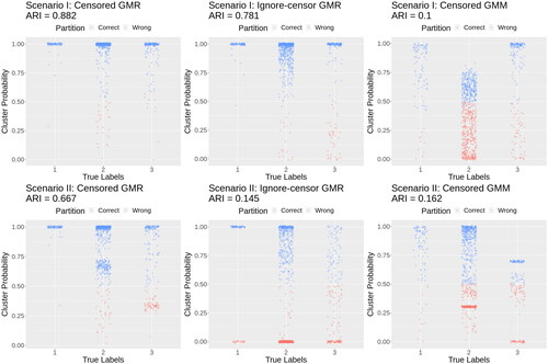
These results highlight the need to model both the censoring and the predictors using the censored multivariate GMR. Even if a study is not interested in the influence of predictors, a mixture of regressions is necessary for accurate clustering. Moreover, the censoring must be modeled, otherwise both clustering and regression coefficient estimates are highly inaccurate.

In Scenarios I and II, all type-1 error rates are near nominal levels, with the highest type-1 error rate equal to 0.056 (Web Supplement Table S.1).

The ICL of the three-cluster model was in general lowest for both Scenarios I and II (Web Supplement Figure S.2). In Scenario I in which censoring levels are similar to our data application, three clusters are selected in 101/101 of simulations. In Scenario II in which censoring is severe, three clusters are selected in 93/101 of simulations.

4. Real Data Application: Emory ADRC/HBS Dataset

The purposes of this analysis are 2-fold: (1) to identify patient clusters based upon their CSF biomarkers without utilizing possibly incorrect clinical diagnoses; and (2) to evaluate the within-cluster effects of the predictors on the CSF biomarkers. The Emory ADRC/HBS Dataset contains 3004 individuals including 888 individuals with AD, 661 individuals with other cognitive disorders (Other), and 1455 individuals who are cognitively normal (CN). Diagnosis is based on a combination of clinical history, neuropsychological testing, blood tests, structural neuroimaging, and CSF biomarkers. All individuals included in our analyses provided informed consent to participate in research protocols approved by the Emory University Institutional Review Board (EHBS IRB00080300, ADRC IRB00079069, NeuCog IRB00078273, Vascular IRB00084414, CRIN IRB00024959). All CSF samples are assayed on the Roche Elecsys platform to measure levels of amyloid-beta peptide 1–42 (Abeta42), total tau protein (tTau), and phosphorylated tau protein (pTau). Because of the detection limits of the biometric assay, the CSF biomarkers are subject to censoring: 10/3004 observations of Abeta42 are left censored and 349/3004 observations are right censored; 31/3004 observations of tTau are left censored and 4 are right censored; and 110/3004 observations of pTau are left-censored and 5 are right censored (Figure 2, see also Figure S.4 for a version stratified by gender, Table 4). Lower CSF Abeta42 corresponds to higher brain Abeta42 burden, such that we expect Abeta42 to be lower in patients with AD. In contrast, higher CSF tTau and pTau are associated with higher tau in the brain, and thus we expect tTau and pTau to be higher in patients with AD. A common approach is to use the ratio of Abeta42/tTau or Abeta42/pTau, where small values indicate AD pathology (Hampel et al. 2008; Meyer et al. 2010). However, using ratios obscures the censoring and discards information available from the multivariate approach. Since ignoring censoring led to erroneous clustering in our simulations, we believe the multivariate approach with the censored multivariate GMR will better reflect the underlying biology.

Figure 2. CSF biomarker data from the Emory ADRC/HBS Study. The diagonals represent histograms of the CSF biomarkers, the lower off-diagonals are scatterplots, and the upper off-diagonals are the Pearson correlations with *** denoting p-value <0.001.

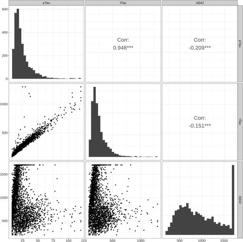
Table 4. Patient demographics of the Emory Goizueta Alzheimer’s Disease Research Center and the Emory Healthy Brain Study Dataset.

Variable		N = 3004
Abeta42:		869.4 (587.2, 1291.0)
	Number of left-censored subjects (< 200):	10 (0.3%)
	Number of right-censored subjects (>1700):	349 (11.6%)
tTau:		206.2 (153.7, 288.3)
	Number of left-censored subjects (< 80):	31 (1.0%)
	Number of left-censored subjects (>1300):	4 (0.1%)
pTau:		17.84 (13.10, 26.78)
	Number of left-censored subjects (< 8):	110 (3.7%)
	Number of right-censored subjects (> 120):	5 (0.2%)
Clinical Diagnosis:
	Alzheimer’s disease (AD):	888 (30%)
	Other cognitive disorders (Other):	661 (22%)
	Cognitively normal (CN):	1455 (48%)
Age (decades)		6.61 (5.94, 7.18)
Educ (decades)		1.60 (1.40, 1.80)
Race:
	American Indian or Alaska Native:	6 (0.2%)
	Asian:	36 (1.2%)
	Black or African American:	495 (16.5%)
	White:	2454 (81.7%)
	Native Hawaiian or Other Pacific Islander:	7 (0.2%)
	Other:	6 (0.2%)
Gender:
	Female:	1788 (59.5%)
	Male:	1216 (40.5%)
ApoE4:
	$\epsilon 4/\epsilon 4:$	193 (6.4%)
	$\epsilon 3/\epsilon 4$ or $\epsilon 2/\epsilon 4:$	900 (30.0%)
	$\epsilon 4$ Negative:	1520 (50.6%)
	missing data:	391 (13.0%)

For continuous variables, we report the median (first quartile, third quartile); for factors, we report the count (percentage).

The data include age (decades),ducationn level (decades), self-reported race, gender, and apolipoprotein E genotype. Due to small sample sizes in American Indian or Alaska Native (n = 6), Asian (n = 36), and Native Hawaiian or Other Pacific Islander (n = 7), we created a binary variable for race equal to one if the participant was African American and zero otherwise. We also conducted the analysis on the dataset restricted to African American and White individuals. The results were nearly equivalent and are included in the Web Supplement Figure S.5. Additionally, there were 82 self-report Hispanic or Latino participants, which was not examined due to sample size. We included four levels: negative for the $\epsilon 4$ allele, heterozygous ApoE4 (ApoE4-1), homozygous ApoE4 (ApoE4-2), and missing data (Table 4).

To select the optimal number of clusters, we calculate the ICL for the number of clusters $G=1,\dots ,6.$ For each G, we estimate an intercept and regression coefficients for the five demographic variables for the three CSF biomarkers, and we estimate the 3 × 3 covariance matrices. The model is randomly initialized 50 times and the solution with the highest likelihood among the set of converged solutions is selected (50/50 iterations converge for G = 1–4, 45/50 for G = 5, and 35/50 for G = 6).

The optimal number of clusters identified by ICL is equal to three (Web Supplement Figure S.3).

To gain insight into the meaning of these groups, we visualize their relationship with the three (possibly incorrect) clinical diagnoses (Figure 3). Panel A shows a scatterplot of Abeta42 and tTau colored by diagnosis group. Panel D shows the same scatterplot colored by the censored multivariate GMR clusters. Panels B and E show Abeta42 vs. pTau for the AD-diagnosis and censored multivariate GMR, respectively, and Panels C and F show tTau vs. pTau for AD-diagnosis and the censored multivariate GMR, respectively.

Figure 3. Scatter plots and violin plots of the diagnosis vs. the clusters identified with G = 3. The top row (A–C) has points colored by the diagnosis labels. The middle row (D–F) has points colored by the clusters estimated in the censored GMR, in which the CSF biomarkers formed a multivariate response with predictors age, education, gender, race, and APOE4. The bottom row (G–I) shows violin plots with side-by-side comparisons of the 3 CSF biomarkers between the clinical diagnostic groups and the model estimated clusters, namely: AD vs. AD-like, Normal vs. Control-like, and Other vs. Non-AD pathology. The cluster descriptions “AD-like,” “Control-like” and “Non-AD pathology” were determined by inspecting the characteristics of each cluster; see text.

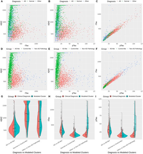
We see that the AD labels in Panels A and B (pink) coincide with the pink censored multivariate GMR cluster in Panels D and E. Thus, we call the pink cluster in Panels D–F the “AD-like pathology” group.

The green group in Figure 3(D–F) tends to coincide with the “Normal” group in Panels A–C. We call this the “control-like” group.

We call the blue group in Figure 3(D–F) the “Non-AD pathology” group. The intercept in Table 5 indicates high CSF Abeta42 compared to control-like, i.e. low Abeta brain burden, which is generally considered non-AD pathology. However, the CSF tTau and pTau levels are higher than both the AD-like and control-like groups, indicating high tau brain burden, which may be associated with other types of dementia or neurological impairment. This group is distinct from the “Other” diagnosis which includes CSF from patients who were diagnosed with other specific conditions (e.g. frontotemporal dementia, Lewy body dementia, and vascular dementia). Most participants in the “Other” group are Control-like in our model as the levels of Abeta42, tTau, and pTau exclude the presence of AD pathology. Those in the “Other” group that are AD-like in our model may represent individuals who were misdiagnosed with a non-AD diagnosis or patients who have mixed pathologies (e.g. combination of AD and vascular pathology). Participants with very high tTau and pTau levels are diagnosed with AD in the clinic but are classified as non-AD pathology in our model, in particular for patients with tTau >500 and pTau >60. Indeed, the tails of the tTau and pTau distributions in our AD-like cluster do not resemble the extreme values in the tail of the AD group (Figures 3(H,I)). This may be a limitation of our Gaussian model. Alternatively, it may be indicative of a distinct biomarker profile for non-AD dementia.

Table 5. Estimated coefficient matrices.

	Abeta42	tTau	pTau
Group 1: AD-like	${\omega }_1=0.370$ (N = 1065)
Intercept	632.55***	260.22***	24.57***
Age (decades)	3.79	29.65***	3.35***
Edu (decades)	18.84	−18.77	−1.7
Female	31.6*	18.26*	1.29
African American	−59.1*	−63.95***	−6.53***
Apoe4-2	−140.69***	87.35***	9.51***
Apoe4-1	−23.41	53.68***	6.19***
Apoe4 missing	−72.22***	29.54*	3.83**
Group 2: Control-like	${\omega }_2=0.577$ (N = 1797)
Intercept	1284.74***	179.31***	15.43***
Age (decades)	−58.96***	11.76***	1***
Edu (decades)	9.84	−2.28	−0.07
Female	111.74***	7.45**	0.66*
African American	−190.45***	−26.57***	−2.24***
Apoe4-2	−684.8***	0.32	0.55
Apoe4-1	−260.1***	−0.56	−0.07
Apoe4 missing	−222.31***	−1.33	−0.45
Group 3: Non-AD pathology	${\omega }_3=0.053$ (N = 142)
Intercept	1116.67***	556.61***	53.79***
Age (decades)	28.33	4.54	1.98
Edu (decades)	260.32	−47.64	−4.97
Female	−9.66	22.83	0.78
African American	350.04	−245.07	−23.48
Apoe4-2	−627.41	281.46*	20.89
Apoe4-1	−156.82	32.89	2.64
Apoe4 missing	62.93	66.62	−5.24

The N after the mixing proportion indicates the number of participants in the cluster according to their maximum posterior probabilities. With *p < 0.05; **p < 0.01; ***p < 0.001, uncorrected.

4.1. Group 1: AD-Like Pathology

Abeta42 levels in African American participants are similar to the group composed of other races, while tTau and pTau are significantly lower in African American participants (Table 5, Figure 4). A low ratio of Abeta42 to tTau is often used to classify individuals as AD. In this AD group, the Abeta42/tTau ratio for an African American participant would be larger than other races, implying that the conventional ratio would potentially misclassify African American patients. The effect of being an African American individual on tTau and pTau is similar to decreasing age by 18 years (Table 5).

Figure 4. Bar plots of the Z-scores of the estimated within-cluster effects of the predictors in the selected G = 3 model. The low Abeta42 high tau group has the greatest overlap with AD diagnosis. The high Abeta42 low tau group has the greatest overlap with cognitively normal. The high Abeta42 and high tau group have mixed pathology, which includes some MCI and other diagnoses. The dashed horizontal lines are the critical Z-score subject to Bonferroni correction for 63 comparisons.

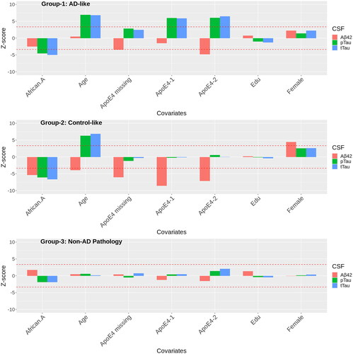
There are large effects of ApoE4 for all three biomarkers, where ApoE4 decreases CSF Abeta42 and increases pTau and tTau. The coefficients for ApoE4-2 are all greater in magnitude than ApoE4-1 (Table 5). Carriers of two copies of ApoE4 have much higher levels of tTau and pTau in the AD-like group compared to carriers of two copies of ApoE4 in the control-like group. The coefficient for APOE4 missing (patients in which these data were not collected) is larger than APOE4-1. Upon further investigation, the missingness in APOE4 is not random: ∼40% are diagnosed with AD and 38% with other pathology, suggesting that the frequency of APOE4-2 may be elevated in this group relative to the observed frequencies.

Other notable findings in this group are no association between age and Abeta42, but a positive relationship with tTau and pTau. Compared to other groups, the coefficients of age on tTau and pTau are large, which reflects a faster progressing tau pathology in the AD group.

4.2. Group 2: Control-Like

In contrast to the AD-like group, CSF Abeta42 is significantly lower in African American participants compared to the group composed of other races in the control-like group. Total tau and pTau are also significantly decreased in African American participants, but the coefficients are smaller than in the AD-like group. Additionally, females in the control-like group had significantly higher levels of CSF Abeta42 than males.

Carriers of ApoE4 have greatly reduced CSF Abeta42, but in contrast to the AD-like group, the tau levels are unchanged. Previous studies have found that ApoE4 is associated with Abeta42 but not tau in cognitively normal aging (Morris et al. 2010).

In contrast to the “AD-like pathology” group, CSF Abeta42 decreases with age (leading to an increase in brain Abeta42) in the control-like group. Since the levels of CSF Abeta42 levels are much lower at baseline in the AD-like group, CSF Abeta42 levels in the control-like group are still higher than the AD-like group at higher ages. Total tau and pTau increase with age, but at a slower rate compared to the AD-like group, which reflects age-progressing tau pathology in the control-like group.

4.3. Group 3: Non-AD Pathology

Overall, we do not see significant relationships between the predictors and CSF biomarkers in this group (Table 5, Figure 4). This may be due in part to the smaller mixing proportion implying a small sample size and imprecise coefficient estimates.

5. Discussion

We used a censored multivariate Gaussian mixture of regressions with a feasible EM algorithm to examine predictor impacts on subgroups in CSF biomarkers of Alzheimer’s Disease. The approach is similar to estimating multivariate regression effects in which all predictors interact with a group variable, but here we also learn the group labels. Our approach simultaneously identifies clusters while allowing the effects of predictors to differ for different clusters for a multivariate outcome with detection limits. In contrast to intensive bootstrap methods, we approximate the asymptotic covariance matrix of the within-cluster effects ${\mathit{\beta }}_g$ using the empirical complete score function. Our simulations show that this approach adequately controls type-1 error rates in large samples (n ≈ 1000). In simulations with moderate (comparable to our data application) and severe censoring, we show that ignoring censored records, deleting censored records, or ignoring predictors creates substantial inaccuracies. Our approach results in large improvements in both the accuracy of clustering and regression estimates. Our simulations add to the latent class literature by demonstrating that modeling both the censoring and the predictors is important for accurate clustering.

Our analysis of the Emory ADRC/HBS Dataset using the censored multivariate GMR reveals new insights. We identify three clusters that tend to align with an AD-like group, a control-like group, and a third group with undefined non-AD pathology. Predictor effects vary across clusters. African American participants in the AD-like group had less severe tTau and pTau pathology. CSF biomarkers typically use the ratio of Abeta42 to tau, but previous studies may have based such determinations on studies of non-Hispanic Whites (Meyer et al. 2010). Recently, some researchers reported potential racial differences in CSF biomarkers (Garrett et al. 2019; Morris et al. 2019), which aligns with our findings. From a clinical perspective, African American participants in the AD-like group likely have AD, yet have a lower tau burden and may be less likely to be diagnosed with AD. This suggests tau may not be a good biomarker for AD among African American individuals. Additionally, tTau and pTau were significantly lower in African American individuals than other individuals in the control-like group. This again suggests that AD pathology differs in African American participants, and underscores the importance of the mixture of regressions approach. The effects of ApoE4 on CSF biomarker levels differed between the AD-like and control-like groups, females had higher CSF Abeta42 than males in the control-like group, and there were no age impacts on Abeta42 in the AD-like group but significant effects in the control-like group, and age impacts on pTau and tTau were greatest in the AD-like group.

Since no gold standard exists for the diagnosis of AD, our unsupervised approach can potentially improve the classification of AD over simple cutoffs from demographically imbalanced studies. Imaging and CSF biomarkers are now used to support diagnosis, although there are issues. PET imaging involves radioactive tracers, is costly, and is commonly not covered by insurance (Chételat et al. 2020; Maschke and Gusmano 2017). Post-mortem studies indicate a high correspondence between Abeta PET and AD pathology but are based on small samples from individuals of European ancestry (Klunk et al. 2004; Seo et al. 2017). Although useful, a positive Abeta PET scan is not equivalent to a clinical diagnosis of Alzheimer’s disease (Kolanko et al. 2020). 18F-FDG PET is also related to AD pathology, although post-mortem studies indicate variable findings with respect to specificity (Fleisher et al. 2020). CSF biomarkers are less costly than PET and avoid the side effects of radioactive tracers.

Although additional research is necessary, our results raise possible issues with current approaches to CSF biomarkers, since cutoffs from CSF biomarkers ignore predictor impacts and multivariate patterns. Our approach found a higher proportion of patients in the AD-like group than were diagnosed with AD. This is expected since there is a significant number of cognitively normal individuals with asymptomatic AD (Jansen et al. 2022, 2015). The multivariate approach with predictors can, in theory, be used to identify asymptomatic AD, which could allow earlier pharmacological interventions. Additional research is necessary to determine whether the AD-like participants identified by our model who are not currently diagnosed with AD later convert to AD. We acknowledge that reducing the CSF biomarkers to three clusters is an over-simplification of a complicated pathology. On the other hand, our approach allows the calculation of patient-specific posterior probabilities, which can help when assessing the strength of evidence for membership in the AD-like group. We are currently investigating an interactive tool to allow a clinician to enter a patient’s data and obtain probabilities for membership in the AD-like, control-like, and non-AD pathology groups. Such a tool holds promise for improving future AD diagnosis and will require careful validation using additional cohorts and longitudinal designs.

There are several limitations to our approach. Our inferential procedure is valid for a known number of clusters. In practice, we select the number of clusters using ICL (Biernacki et al. 2000). This creates issues with post-selection inference (Fithian et al. 2017) since our inference depends on selecting the correct number of clusters. This problem would be made worse if one were to also try to select which predictors to include, so we recommend a priori fixing the predictors to be included in all clusters, as in our application. ICL selected the true number of clusters for all simulations with censoring levels comparable to the data application (100% of Scenario I simulations) and in most simulations with severe censoring (92% of Scenario II simulations). If too many clusters are used, then between-group differences may be lessened, corresponding to fewer significant group differences. Model selection and interpretation can be challenging with an increasing number of response variables, predictors, and groups. Penalized approaches may be helpful in higher dimensions (Khalili and Lin 2013; Xie et al. 2010). Another avenue for future research is to consider an alternative approach that models the probability of latent class membership as a function of covariates using multinomial regression (Jacobs et al. 1991). In our approach, the predictors indirectly impact the posterior probabilities. This results in more interpretable effects, which can deepen our understanding of the impact of demographics, behavior, and genetics on biomarkers in complex neurological disorders.

Software

The code used in Section 3 is available at https://github.com/GanzhongTian/CensGMR.

Acknowledgments

We would like to thank two anonymous referees for their helpful feedback.

Disclosure Statement

J. Lah is a consultant for Roche Diagnostics.

Additional information

Funding

G.T. was supported by R01 AG055634 and R01 AG070937. B.B.R. was supported by R21 AG066970. J.H. was supported by R01 AG055634 and P30 AG066511. J.L. was supported by R01 AG070937 and P30 AG066511. Funding for materials for Roche Elecsys assays were supported by a Roche IIS grant RD004723 to J.L. Additional funding for this work was provided by a generous gift from the Goizueta Foundation.

References

- Amemiya T. 1973. Regression analysis when the dependent variable is truncated normal. Econometrica. 41(6):997.
- Benaglia T, Chauveau D, Hunter DR, Young DS. 2009. mixtools: An R package for analyzing mixture models. J Stat Soft. 32(6):1–29.
- Biernacki C, Celeux G, Govaert G. 2000. Assessing a mixture model for clustering with the integrated completed likelihood. IEEE Trans Pattern Anal Machine Intell. 22(7):719–725.
- Blennow K, Dubois B, Fagan AM, Lewczuk P, De Leon MJ, Hampel H. 2015. Clinical utility of cerebrospinal fluid biomarkers in the diagnosis of early Alzheimer’s disease. Alzheimers Dement. 11(1):58–69.
- Caudill SB. 2012. A partially adaptive estimator for the censored regression model based on a mixture of normal distributions. Stat Methods Appl. 21(2):121–137.
- Chételat G, Arbizu J, Barthel H, Garibotto V, Law I, Morbelli S, van de Giessen E, Agosta F, Barkhof F, Brooks DJ, et al. 2020. Amyloid-pet and 18f-fdg-pet in the diagnostic investigation of Alzheimer’s disease and other dementias. Lancet Neurol. 19(11):951–962.
- Coates A, Ng AY. 2012. Learning feature representations with K-means. In: Montavon G, Orr GB, Müller KR, editors. Neural networks: tricks of the trade, chapter 22. 2nd ed. Berlin; Heidelberg: Springer. p. 561–580.
- Collins J, Huynh M. 2014. Estimation of diagnostic test accuracy without full verification: a review of latent class methods. Stat Med. 33(24):4141–4169.
- De Alencar F, Galarza C, Matos L, Lachos V. 2020. CensMFM: finite mixture of multivariate censored/missing data. R Package Version 2. https://CRAN.R-project.org/package=CensMFM
- Dubois B, Feldman HH, Jacova C, Dekosky ST, Barberger-Gateau P, Cummings J, Delacourte A, Galasko D, Gauthier S, Jicha G, et al. 2007. Research criteria for the diagnosis of Alzheimer’s disease: revising the NINCDS–ADRDA criteria. Lancet Neurol. 6(8):734–746.
- Fair RC. 1977. A note on the computation of the Tobit estimator. Econometrica. 45(7):1723.
- Fithian W, Sun D, Taylor J. 2017. Optimal inference after model selection. arXiv preprint arXiv:1410.2597.
- Fleisher AS, Pontecorvo MJ, Devous MD, Lu M, Arora AK, Truocchio SP, Aldea P, Flitter M, Locascio T, Devine M, et al. 2020. Positron emission tomography imaging with [18f] flortaucipir and postmortem assessment of Alzheimer disease neuropathologic changes. JAMA Neurol. 77(7):829–839.
- Galarza CE, Kan R, Lachos VH. 2021. MomTrunc: moments of folded and doubly truncated multivariate distributions. R Package Version 5.97. https://CRAN.R-project.org/package=MomTrunc
- Garay A, Lachos V, Massuia M. 2013. SMNCensReg: fitting univariate censored regression model under the scale mixture of normal distributions. R Package Version 2. https://CRAN.R-project.org/package=SMNCensReg
- Garay AM, Lachos VH, Bolfarine H, Cabral CR. 2017. Linear censored regression models with scale mixtures of normal distributions. Stat Papers. 58(1):247–278.
- Garrett SL, McDaniel D, Obideen M, Trammell AR, Shaw LM, Goldstein FC, Hajjar I. 2019. Racial disparity in cerebrospinal fluid amyloid and tau biomarkers and associated cutoffs for mild cognitive impairment. JAMA Netw Open. 2(12):e1917363.
- Goetz ME, Hanfelt JJ, John SE, Bergquist SH, Loring DW, Quyyumi A, Clifford GD, Vaccarino V, Goldstein F, Johnson TM, et al. 2019. Rationale and design of the Emory Healthy Aging and Emory Healthy Brain Studies. Neuroepidemiology. 53(3–4):187–200.
- Goldfeld SM, Quandt RE. 1973. A Markov model for switching regressions. J Econom. 1(1):3–15.
- Hahsler M, Piekenbrock M, Doran D. 2019. dbscan: fast density-based clustering with R. J Stat Soft. 91(1):1–30.
- Hampel H, Bürger K, Teipel SJ, Bokde AL, Zetterberg H, Blennow K. 2008. Core candidate neurochemical and imaging biomarkers of Alzheimer’s disease. Alzheimers Dement. 4(1):38–48.
- Hanson T, Johnson WO. 2002. Modeling regression error with a mixture of Polya trees. J Am Stat Assoc. 97(460):1020–1033.
- Jacobs RA, Jordan MI, Nowlan SJ, Hinton GE. 1991. Adaptive mixtures of local experts. Neural Comput. 3(1):79–87.
- Jansen WJ, Janssen O, Tijms BM, Vos SJB, Ossenkoppele R, Visser PJ, Aarsland D, Alcolea D, Altomare D, von Arnim C, et al. 2022. Prevalence estimates of amyloid abnormality across the Alzheimer disease clinical spectrum. JAMA Neurol. 79(3):228–243.
- Jansen WJ, Ossenkoppele R, Knol DL, Tijms BM, Scheltens P, Verhey FRJ, Visser PJ, Aalten P, Aarsland D, Alcolea D, et al. 2015. Prevalence of cerebral amyloid pathology in persons without dementia: a meta-analysis. JAMA. 313(19):1924–1938.
- Jedidi K, Ramaswamy V, Desarbo WS. 1993. A maximum likelihood method for latent class regression involving a censored dependent variable. Psychometrika. 58(3):375–394.
- Karlsson M, Laitila T. 2014. Finite mixture modeling of censored regression models. Stat Papers. 55(3):627–642.
- Khalili A, Lin S. 2013. Regularization in finite mixture of regression models with diverging number of parameters. Biometrics. 69(2):436–446.
- Klunk WE, Engler H, Nordberg A, Wang Y, Blomqvist G, Holt DP, Bergström M, Savitcheva I, Huang G-F, Estrada S, et al. 2004. Imaging brain amyloid in Alzheimer’s disease with Pittsburgh compound-b. Ann Neurol. 55(3):306–319.
- Kolanko MA, Win Z, Loreto F, Patel N, Carswell C, Gontsarova A, Perry RJ, Malhotra PA. 2020. Amyloid pet imaging in clinical practice. Pract Neurol. 20(6):451–462.
- Lee G, Scott C. 2012. EM algorithms for multivariate Gaussian mixture models with truncated and censored data. Comput Stat Data Anal. 56(9):2816–2829.
- Leisch F. 2004. FlexMix: a general framework for finite mixture models and latent class regression in R. J Stat Softw. 11(8):1–18.
- Linzer DA, Lewis JB. 2011. poLCA: an R package for polytomous variable latent class analysis. J Stat Soft. 42(10):1–29.
- Maschke KJ, Gusmano MK. 2017. Medicare and amyloid pet imaging: the battle over evidence. J Aging Soc Policy. 29(2):105–122.
- McKhann G, Drachman D, Folstein M, Katzman R, Price D, Stadlan EM. 1984. Clinical diagnosis of Alzheimer’s disease: report of the NINCDS-ADRDA Work Group* under the auspices of department of health and human services task force on Alzheimer’s disease. Neurology. 34(7):939–944.
- McKhann GM, Knopman DS, Chertkow H, Hyman BT, Jack CR Jr., Kawas CH, Klunk WE, Koroshetz WJ, Manly JJ, Mayeux R, et al. 2011. The diagnosis of dementia due to Alzheimer’s disease: recommendations from the national institute on aging-Alzheimer’s Association Workgroups on Diagnostic Guidelines for Alzheimer’s disease. Alzheimers Dement. 7(3):263–269.
- McLachlan GJ, Peel D. 2000. Finite mixture models. New Jersey: Wiley.
- Meyer GD, Shapiro F, Vanderstichele H, Vanmechelen E, Engelborghs S, Deyn PPD, Coart E, Hansson O, Minthon L, Zetterberg H, et al. 2010. Diagnosis-independent Alzheimer disease biomarker signature in cognitively normal elderly people. Arch Neurol. 67(8):949–956.
- Morris JC, Roe CM, Xiong C, Fagan AM, Goate AM, Holtzman DM, Mintun MA. 2010. APOE predicts amyloid-beta but not tau Alzheimer pathology in cognitively normal aging. Ann Neurol. 67(1):122–131.
- Morris JC, Schindler SE, McCue LM, Moulder KL, Benzinger TL, Cruchaga C, Fagan AM, Grant E, Gordon BA, Holtzman DM, et al. 2019. Assessment of racial disparities in biomarkers for Alzheimer disease. JAMA Neurol. 76(3):264–273.
- O’Hagan A, Murphy TB, Scrucca L, Gormley IC. 2019. Investigation of parameter uncertainty in clustering using a Gaussian mixture model via jackknife, bootstrap and weighted likelihood bootstrap. Comput Stat. 34(4):1779–1813.
- Quandt RE, Ramsey JB. 1978. Estimating mixtures of normal distributions and switching regressions. J Am Stat Assoc. 73(364):730–738.
- Ruud PA. 1991. Extensions of estimation methods using the EM algorithm. J Econom. 49(3):305–341.
- Sanchez LB, Lachos VH, Moreno EJL, Sanchez MLB, LazyData T. 2018. Package ‘censmixreg’. R package version 3.1.
- Scrucca L, Fop M, Murphy TB, Raftery AE. 2016. mclust 5: Clustering, classification and density estimation using Gaussian finite mixture models. R J. 8(1):289–317.
- Seo SW, Ayakta N, Grinberg LT, Villeneuve S, Lehmann M, Reed B, DeCarli C, Miller BL, Rosen HJ, Boxer AL, et al. 2017. Regional correlations between [11c] pib pet and post-mortem burden of amyloid-beta pathology in a diverse neuropathological cohort. Neuroimage Clin. 13:130–137.
- Shin J, Doraiswamy PM. 2016. Underrepresentation of African-Americans in Alzheimer’s trials: a call for affirmative action. Front Aging Neurosci. 8:123.
- Vermunt JK, Magidson J. 2021. Lg-syntax user’s guide: manual for latent gold syntax module version 6.0. Arlington (MA): Statistical Innovations Inc.
- Wang WL, Castro LM, Hsieh WC, Lin TI. 2021. Mixtures of factor analyzers with covariates for modeling multiply censored dependent variables. Stat Papers. 62(5):2119–2145.
- Wang WL, Castro LM, Lachos VH, Lin TI. 2019. Model-based clustering of censored data via mixtures of factor analyzers. Comput Stat Data Anal. 140:104–121.
- Xie B, Pan W, Shen X. 2010. Penalized mixtures of factor analyzers with application to clustering high-dimensional microarray data. Bioinformatics. 26(4):501–508.
- Yuksel SE, Wilson JN, Gader PD. 2012. Twenty years of mixture of experts. IEEE Trans Neural Netw Learn Syst. 23(8):1177–1193.
- Zeller CB, Cabral CRB, Lachos VH, Benites L. 2019. Finite mixture of regression models for censored data based on scale mixtures of normal distributions. Adv Data Anal Classif. 13(1):89–116.