Accuracy of available methods for quantifying the heat power generation of nanoparticles for magnetic hyperthermia

Abstract

In magnetic hyperthermia, characterising the specific functionality of magnetic nanoparticle arrangements is essential to plan the therapies by simulating maximum achievable temperatures. This functionality, i.e. the heat power released upon application of an alternating magnetic field, is quantified by means of the specific absorption rate (SAR), also referred to as specific loss power (SLP). Many research groups are currently involved in the SAR/SLP determination of newly synthesised materials by several methods, either magnetic or calorimetric, some of which are affected by important and unquantifiable uncertainties that may turn measurements into rough estimates. This paper reviews all these methods, discussing in particular sources of uncertainties, as well as their possible minimisation. In general, magnetic methods, although accurate, do not operate in the conditions of magnetic hyperthermia. Calorimetric methods do, but the easiest to implement, the initial-slope method in isoperibol conditions, derives inaccuracies coming from the lack of matching between thermal models, experimental set-ups and measuring conditions, while the most accurate, the pulse-heating method in adiabatic conditions, requires more complex set-ups.

• Calorimetric methods
• magnetic hyperthermia
• magnetic methods
• magnetic nanoparticles
• specific absorption rate

Introduction

The success in the use of a particular material for a given application is based on three main aspects: the adequate synthesis or fabrication of such materials, the correct characterisation of their specific functionalities, and the assessment of their performance in operating conditions. Since the first reported experiments on tissue heating using maghemite nanoparticles exposed to a 1.2-MHz magnetic field [1], this statement has been implemented with nano-objects based on magnetic nanoparticles (MNPs) to be used as the active principle in the application of magnetic fluid hyperthermia (MFH) for cancer treatment [2,3]. The number of research groups working on synthesis [4–6], encapsulation [7,8] and functionalisation [9,10] of such nano-objects has increased exponentially. Some of these materials have been subjected to biological tests, such as studies on cellular uptake [11] and cell viability upon MFH sessions [12], assessments of in vivo tumor regression [13–16] and clinical trials [17–21]. In particular, the company Magforce (Berlin, Germany) has been a pioneer in obtaining the European Union Regulatory Approval (10/2011) to perform the NanoTherm® therapy on glioblastoma multiforme at the Charité Hospital in Berlin.

The NanoTherm® therapy [22] is performed in three steps: (1) injection of the ferrofluid into the tumour, (2) therapy planning according to the MNP distribution within the tumour, previously observed by CT, (3) therapy application using a special-purpose alternating magnetic field (AMF) applicator [23,24], which operates at a fixed frequency, f, of 100 kHz and at variable amplitude, H₀, ranging from 2 to 18 kA/m.

The planning of the therapy is performed by means of special-purpose software that uses the bioheat transfer equation to simulate the maximum temperatures achieved during the treatment, which allows the defining of the AMF amplitude and the duration of the sessions. Simulations require quantification of several parameters [25,26], either geometrical (e.g. MNP distribution), physiological (e.g. blood pressure) or thermal, both of the tissues (e.g. specific heat) and of the MNPs (e.g. heat power generation upon AMF application). The latter in particular, which is the specific functionality of MNPs for MFH, is quantified by means of the specific absorption rate, SAR (W/g), also referred to as specific loss power (SLP), defined as where P is the heat power dissipated by the MNPs and m_MNP is the mass of magnetic material.

Published data describing treatment results [19,20], reflect in some cases differences of several degrees Celsius between the real achieved temperature, measured by invasive thermometry, and the simulated temperature. Most likely sources of these concerning differences are two-fold: first, widely used methods for SAR measurement may derive high inaccuracies, and second, SAR determination is often carried out on ferrofluids, despite that the performance of these systems may differ considerably from that of MNP local arrangements within the tissues after injection, in which heating mechanisms may be reduced or suppressed and where, due to the intrinsic magnetic nature of the MNPs, inter-particle interactions affect their magnetic properties and may degrade SAR values. In this sense, a more accurate determination of SAR on more adequate arrangements (e.g. solid matrices, phantoms, biopsies) would improve matching between simulations and real temperatures during therapies.

The correct determination of SAR is not only relevant for the planning of therapies, but also to feedback synthetic procedures leading to optimising the performance of these materials, and to correlating SAR with the different dissipation mechanisms and characteristics of MNPs arrangements, so that optimisation of materials can be more easily fulfilled [11].

Given that the SAR of a given MNP system with given size distribution, spatial arrangement, add-ons and dispersive media is an intrinsic property, one should obtain the same SAR value independently of the measuring method employed for its determination, so that differences between methods are indicative of the presence of uncertainties. In this work we survey the different methods currently used for SAR determination, discussing derived uncertainties, as well as their sources and possible minimisation.

Inaccuracies related to alternating magnetic field

The heating generated by MNPs under an AMF is strongly dependent on H₀. It is thus of crucial importance that the AMF used in any set-up for SAR measurement has a constant and well-known amplitude at the sample space, so that the sample heating output can be assigned to this H₀ value. This should be ensured by careful designs of the AMF source and corroborated by simulations [27–30]. It is also important to minimise the influence of the eventual heating of the AMF source on the sample, for example, using vacuum, an insulator layer or cooling means [28,31]. Furthermore, a magnetised sample placed within the generated AMF tends to decrease the magnetic field inside itself through the so-called demagnetising field, which is determined by the shape of the sample, and is more relevant the higher its magnetisation (M) is. This effect derives inaccuracies in the determination of H₀ if appreciable unknown and non-constant H₀ distributions are generated inside the sample volume [32,33].

SAR increases with f and H₀, since more energy is transferred from the AMF to the MNPs. It is straightforward then, thinking that by increasing f and H₀, the higher heating output of the MNPs would make it possible to reduce the dosage of MNPs supplied to the body, with the same therapeutic effects. However, the values of these parameters that can be safely used at in vivo applications are restricted to a certain range due to unwanted eddy currents generated in the tissue and induced stimulation of peripheral nerves [34]. As a rule of thumb, a product H₀ċf < 485 kA/m kHz (biological range of AMF application) is required in humans [35], with 50 < f < 1200 kHz and H₀ < 15 kA/m, though higher H₀· f products can be applied to certain areas of the body, as shown in Wust et al. [19]. In this study, using f = 100 kHz, the maximum H₀ bearable by the patients was 3–6 kA/m for the pelvis, confirming results in Atkinson et al. [35], while for the head it rose up to more than 10 kA/m. In animal studies the H₀· f frontier is broader [13–16,36].

In spite of the limited values of AMF parameters required for clinical applications, the parameters used for measuring SAR cover a much wider range. This fact is reflected in Figure 1, generated using references [4–11,27–32,37–96] and self-references herein. The majority of SAR determination experiments are in fact performed with pairs (f, H₀) out of the biological range. The most used f is 100 kHz in the case of calorimetric determinations, but the AMF amplitudes are usually higher than 5 kA/m, whereas magnetic determinations tend to apply very low H₀ values, but higher frequencies, reaching the MHz range. In both cases these ranges are somehow imposed by the set-ups used for SAR determination, as will be seen in the following sections. To extrapolate SAR measurements to the f and H₀ values suitable for clinical MFH, a SAR ∝ f·  dependency is widely applied, but this relationship scarcely holds [41,45,46,97]. At most, it can be used to compare the efficiency of several systems in generating heat from the AMF energy, but not to systematically extrapolate SAR values. Even assuming the basic case of a monodisperse MNP system without inter-particle interactions, diverse dependencies on f and H₀ can be found, for example, due to different magnetic behaviours as a function of MNP size [97] (multi-domain, ferro/ferrimagnetic single-domain or superparamagnetic) or depending on the relative value of H₀ compared to that of characteristic magnetic parameters of the system, such as anisotropy field and coercive field [98,99].

Figure 1. Histogram on AMF parameters of research groups measuring SAR from calorimetric or magnetic methods. The height of each column represents the number of research groups that have at least one publication between 2000 and 2012 measuring the SAR at the values of f and H₀ corresponding to the position of the column in the horizontal plane. For example, the column at the position (200 kHz, 3 kA/m) accounts for all the groups using 200–299 kHz and 3–3.9 kA/m. In the central insets, the columns corresponding to the biological range as defined in Atkinson et al. [35] are displayed in white, while the rest are displayed in blue.

These dependencies may be mixed within a system with size dispersion (resulting in an unknown average behaviour) or altered due to inter-particle magnetic interactions [99,100], both being non-negligible in common MNP systems. Consequently, to avoid inaccuracies deriving from extrapolations, the use of parameters within the biological range of AMF application is highly advised.

Magnetic determination of SAR

An assembly of MNPs subjected to an external AMF invests electromagnetic energy from the field in magnetisation reversal processes. Its internal energy is then first increased and afterwards released as heat. The relationship between the heat generated and the magnetic response of the MNPs makes possible the determination of SAR by different types of magnetic measurements, in which this response is usually measured by quantifying, through different sensors, the current induced in a gradiometric inductive coil due to the changes over time in the magnetic flux density produced by the sample [101].

Hysteresis loops

When an AMF is applied to a ferro/ferrimagnetic material, the non-linearity and delay of its magnetisation with respect to the applied field, H, originates that the M versus H trend describes a so-called hysteresis loop. The area entrapped within the M(H) cycle determines the heat dissipated per AMF cycle, and SAR can be calculated from quantification of this area [102] as where µ₀ = 4π × 10⁻⁷T m/A is the permeability of free space, ρ_MNP is the density of the magnetic material, and M and H are expressed in SI units (A/m). According to Equation 2, SAR can be computed by magnetic methods by calculating the value of the closed integral, that is, by determining the area of the hysteresis loop between ±H₀ integrating the experimental M(H) curve and taking into account the AMF frequency.

Several research groups [37–39,98,103–107] calculate this area using vibrating sample magnetometers (VSM) [108] or superconducting quantum interference device (SQUID) magnetometers [109], both being commercial equipment present in many laboratories involved with magnetism. With them, hysteresis loops are carried out quasi-statically, that is, magnetisation is measured in the presence of a magnetic field varying at very low frequency, much smaller than those used for MFH. Accordingly, this method may easily drive to a misleading SAR determination if the effects of AFM frequency on the area of hysteresis loops are not considered.

In particular, this method is useless for superparamagnetic nanoparticles, which show no hysteresis in quasi-static measurements due to thermally activated magnetisation relaxation mechanisms, whereas the area of dynamic loops at certain frequencies is non-zero and frequency dependent for such materials [41,45,49,97]. Single-domain MNPs out of the superparamagnetic regime and multi-domain MNPs do present quasi-static hysteresis, but the area of these loops differ from those obtained with higher frequencies [110,111].

To avoid uncertainties derived from frequency effects, the ideal option is to determine the area of hysteresis loops applying AMFs with the typical parameters for MFH. To the authors’ knowledge, there is no commercial equipment committed to the measurement of M(H) cycles in the biological range of AMF application, as the detection of magnetisation at frequencies in the range of the kHz brings several problems [108]. However, some groups have developed such home-made devices [28,40–45]. It is worth highlighting the device in Bekovic et al. [28,43] which measures temperature while recording M(t) and H(t) during AMF application at typical f and H₀ for MFH (50–678 kHz, up to 15 kA/m). This set-up allowed comparison between SAR values determined simultaneously by calorimetric methods and by hysteresis-loop integration [28]. In that work, the standard deviation of the values obtained calorimetrically were found bigger, due to the calorimetric method used (see Use of time constant and ΔT_max below).

AC magnetic susceptibility

In linear response theory (LRT) the magnetisation of an assembly of MNPs is assumed to be linear with H, with a complex magnetic susceptibility χ = χ′ − iχ″, where χ′ and χ″ are the in-phase and out-of-phase components of magnetic susceptibility, respectively. In this framework, χ depends on AFM frequency, but not on H₀. Using this complex susceptibility and considering sinusoidal applied magnetic field [102], Equation 2 changes into and provides another method to calculate SAR by magnetic means, using the complex susceptibility of the system provided that LRT can be applied.

According to Carrey et al. [97], where MNP systems with no inter-particle interactions are tackled, LRT is only valid when where M_s is the saturation magnetisation of the material in SI units, V_M is the magnetic volume of each MNP, k_B is the Boltzmann constant and H_k is the anisotropy field. However, as stated in Carrey et al. [97], if SAR values are not negligible, the condition on the right is fulfilled when the condition on the left is, indicating that LRT is only valid in the low field range, and that the maximum H₀ value for LRT validity decreases with increasing V_M.

Some of the most widespread commercial devices for magnetic measurements allow performing χ″ high-sensitivity measurements as a function of T. f and H₀. For example, the PPMS and MPMS from Quantum Design (San Diego, CA), work with f = 10 Hz–10 kHz, H₀ ≤ 1.2 kA/m and f = 0.1 Hz–1 kHz, H₀ ≤ 0.2 kA/m, respectively, but these parameters are not that useful for MFH. Special-purpose high-frequency AC susceptometers have been built [43,46–50,112], with frequencies up to 1 MHz, one of them is currently commercially available [48]. They use H₀ ≤ 0.5 kA/m, with an exception [50], where H₀ reaches 3.2 kA/m. In most cases, the f and H₀ ranges of these set-ups still demand extrapolations in order to predict SAR for MFH applications, with the subsequent inaccuracies. Finally, the system described in Bekovic et al. [43] allows the simultaneous calculation of χ″ and the hysteresis loop area from the temporal evolution of H and M, the SAR obtained with both magnetic methods displaying a good accordance. This device can also determine SAR as a function of T for temperatures above room temperature.

As a final remark applicable to all magnetic methods, in addition to typical experimental considerations for general magnetic measurements (e.g. diamagnetic corrections for sample holders and dispersive media), the T at which the measurement is performed must be considered, since, as SAR depends on T, each obtained value should be assigned to the mean T of each measuring process. Keeping in mind that the MNPs under study are designed for heating applications, some heating is expected during measurements in the sample and in the metallic parts surrounding it, especially in devices without T control.

Calorimetric determination of SAR

Background

Calorimetry, the science of measuring the amount of heat, is the ‘direct’ way to determine SAR. By using calorimetric methods, neither magnetic mechanisms originating heat dissipation, nor data acquisition rates, need to be considered a priori, contrarily to magnetic measurements, since it is the consequence of the magnetic moment reversal that is quantified.

Heat quantification is usually performed through the measurement of the temperature evolution of the sample under study. For that purpose, one must use a set-up allowing the measurement of T, and a thermal model describing such physical system, since the temperature evolution of the sample is a consequence of the balance between the heat generated by the sample and the heat interchanged with its environment, and depends on the thermal properties and geometric characteristics of both the sample and its environment.

It is obvious that the better the thermal model fits the physical system, the more accurate is the determination of heat. But it often happens that the simpler the measuring set-up, the more complicated the thermal model, since it includes many thermal parameters of both the sample and its environment, which vary with space and time, and are difficult to determine.

In a general thermal model for SAR measurement, the sample is initially at the same temperature as its environment, T₀, and the AMF is switched on at t = 0. Given that the sample generates heat upon AMF application, it can be considered a sample with heat sources inside. If we assume that the heat sources (MNPs) are homogeneously distributed across the sample, then the heat power by volume unit is P.V, where V is the volume of the whole sample. The heat generated by the MNPs is diffused across the sample, and the heat flux arriving to the sample limits is continuously transferred to the sample environment (e.g. container, insulator, air) by conduction, convection and radiation. The T distribution inside the sample is governed, for the case of solids and fluids either stationary or in laminar flow, by the heat-propagation equation with heat sources: where ρ. c and κ are, respectively, the mass density, the specific heat (J/g·K) and the thermal conductivity (W/m·K) of the sample, considered homogeneous within the sample, and is the position vector of the different points of the sample. This differential equation in partial derivatives can be solved analytically but, given that such equation derives generally complex analytical solutions, these problems are often tackled with numerical calculations. In both cases, resolution involves using the temporal and the boundary conditions adequate to each case, which depend on the thermal interaction between the sample and its environment. Solutions may reflect temperature gradients across the sample, and also different temporal evolutions for different points of the sample.

The thermal model for SAR measurement is appreciably simplified if the temperature gradients across the sample are neglected, so the sample temperature is considered always homogeneous. This is obviously an idealisation of the system, since a thermal gradient exists inside the sample, given that heat is transferred to the environment. This assumption gives reasonable estimations when the internal (inside the sample) thermal relaxation time is about ten times lower than the external one (sample to its environment) [113]. Both relaxation times depend on thermal and geometrical parameters of the sample and its environment and vary for each experimental set-up. The most suitable case of application would involve a highly conductive sample with a weak thermal link to its environment.

Within this approximation, the power balance between the sample and its environment can be used to infer the temporal evolution of the sample temperature. Considering ideal isoperibol conditions (i.e. the temperature of the sample varies, but the temperature of its environment is always constant), and assuming linear losses between the sample and its environment, this power balance can be written as where C = ∑c_i· m_i, is the heat capacity (J/K) of the sample, obtained as the summation of the products of the mass (m_i) and specific heat (c_i) of all parts integrating the sample, and L(W/K) is a not necessarily constant coefficient accounting for losses. This equation reflects that the temperature rise of the sample is the consequence of the balance between the heat power generated by the MNPs and the heat power lost to the environment.

Equation 6 includes several parameters whose values may undergo significant changes with temperature, namely, C. P and L. However, in most cases, if the temperature interval of the experiment is small (several degrees Celsius), these parameters can be considered independent of T. In such cases, the solution to this differential equation, considering T.t = 0) = T₀ and switching on the AC field at t = 0, is where ΔT_max = P.L, and τ = C.L. In the stationary state, the heat generated and lost become equal, and the sample temperature remains constant at a value T_max = T₀ + ΔT_max.

Starting from this theoretical background, the calorimetric methods currently used for SAR determination are described and their accuracy discussed.

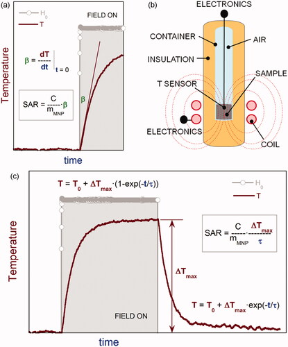
Initial-slope method

The initial-slope method for SAR determination is based on two main assumptions: (1) the sample temperature is always homogeneous while heating upon application of an AMF, and (2) heat losses are negligible during a certain time interval at the beginning of the heating process. According to the first assumption, Equation 7 describes the T-vs-t characteristic of the sample. The derivative of this equation at the onset of heating is and, according to this equation, SAR can be calculated as where the initial slope, β, is calculated within the time interval, Δt, in which heat losses are negligible (see Figure 2A). As stated above, the correct use of Equation 7 also requires the consideration of small temperature intervals, to ensure that P and C are temperature independent. Given that this method uses the initial part of the T-vs-t characteristic, this condition is generally fulfilled. The use of small T intervals would help as well to assure negligible thermal losses.

Figure 2. SAR determination by calorimetric methods in non-adiabatic isoperibol conditions: (A) SAR calculation by the initial-slope (β) method, (B) scheme of a typical experimental set-up, (C) SAR calculation using the parameters ΔT_max (maximum temperature increment) and τ (relaxation time) obtained from the fit of the complete T-vs-t curve to the exponential trend characteristic of isoperibol conditions.

In one of the earliest references of the use of the initial-slope method for SAR determination [114], a special-purpose set-up was fabricated to determine the SAR of iron oxide MNPs suspended in different dispersive media. In it, samples were thermally isolated in a vacuum vessel placed into a circular two-turn coil, and temperature variations were measured by means of a type-T thermocouple (copper/constantan). In that case, the initial slope dT/dt was obtained by linear regression of the T-vs-t trend at the start of heating and SAR was calculated from an equation analogous to Equation 9.

Currently, most of the research groups working on MFH have adopted this initial-slope method [4–6,9,10,29,37–39,41,46,47,51–74,96,107,115,116], most probably due to the relatively easy built-in experimental set-ups (see Figure 2B). Variations of the above-reported set-up have been built in many research laboratories, and few of them are currently commercially available. In these set-ups, AMF is often generated inside cooled (water, air, nonane) copper coils with a number of turns ranging between 2 and 70, although in some cases the AFM is created within the gap of ferrite-core electromagnets [5,46,62,69]. In Chen et al. [116], an orthogonal synchronised bi-directional AMF is reported. Samples are placed in a wide variety of containers: glass or plastic test tubes, twin-walled test tubes, Petri dishes, plastic or glass vials, PCR microtubes, glass capillaries, centrifuge or microcentrifuge tubes, plastic capsules and also special-purpose holders in polypropylene or Teflon, glass flasks with vacuum shield, etc., whose volume is either partially or fully occupied by the sample. The group sample + container is often partially or fully thermally linked with room air by different poor heat-conducting means, such as vacuum vessels, twin-walled glass vessels with air flow, polystyrene or polyurethane foams, asbestos, polypropylene or Teflon. The temperature of the sample is registered by different contact or non-contact sensors, namely thermistors, thermocouples, organic liquid thermometers, pyrometers, IR cameras or fibre-optic probes, the last ones being most common. From the T-vs-t characteristics obtained, data within a certain initial time interval, which varies from several tens of seconds to several minutes, is used to calculate the initial slope, either by differentiation of a fit (linear [41,53,114], polynomial [4,61]) or by direct calculation of ΔT/Δt [38,51,60,66]. Some authors use numerical differentiation and, given that the initial T-vs-t trend is not strictly linear and the slope is non-constant, they use maximum slopes [56,107] or constant slopes [59] to determine SAR. In summary, there is a large variety of set-ups and measuring conditions.

While the greatest advantage of this technique is the relative simplicity of the experimental arrangement, its most important and concerning drawback is the unknown degree of uncertainty of the obtained data. Given that Equation 7 is just a simplified model discarding temperature diffusion across the sample, and that the determination of β takes place most probably at the transient state of the sample temperature, the above assumptions should be verified for the different experimental conditions. Several works accounting for the inaccuracy of this technique are detailed below.

In Jones and Winter [115], microspheres containing different amounts of ferromagnetic material were infused into rabbit kidneys via the renal artery, and T-vs-t characteristics were recorded in vivo for different locations of the temperature sensor, and upon application of an alternating magnetic field generated inside a 15-turn induction coil. The observed trends were found to be exponential, and the initial slope of the T-vs-t trends was described using an equation equivalent to Equation 9. Comparing the experimental dT/dt values with those calculated using the SAR value obtained from VSM measurements, deviations from 0 up to 85% were obtained, mainly assigned to the simplified assumption of homogeneous heating and neglecting of thermal conduction and tissue perfusion, although the inaccuracy of the VSM technique would surely play a role (see Hysteresis loops above).

In Natividad et al. [117], experimental SAR data obtained with the initial-slope method and the pulse heating method (see Pulse heating method below) were compared for different insulating conditions, temperature sensors and sample–sensor contacts. The sample used was constituted by about 0.3 mL of a magnetite-based aqueous ferrofluid inside a quartz container. Using the accurate SAR value obtained by the pulse heating method as a reference (0.72 W/g for f = 109 kHz and H₀ = 2 kA/m), the uncertainties of the initial-slope method were determined. Using as temperature sensor a glued thermocouple, SAR underestimations between 2% and 34% were obtained under different isolation conditions. With polystyrene foam as insulator, and using a pyrometer or a fibre-optics thermometer measuring through the container, underestimations of 48–50% were obtained. And finally, with polystyrene foam as insulator, and a fibre-optics thermometer inside the ferrofluid, the SAR was either overestimated (5%, using a Δt = 40 s for linear regression) or underestimated (12%, using a Δt = 120 s for linear regression).

More recently, numerical simulations of the heating process were performed in order to infer the potential sources of errors in measuring SAR using the initial-slope method [32,118]. Simulations were developed in ideal isoperibol conditions and according to typical experimental set-ups. The main results indicate that the sample volume required to obtain a reduced error must be relatively high (e.g. 2.5 mL or more for a power density of 3.8 W/cm³), but this critical volume varies with other parameters such as specific heat or heat power dissipation level. According to these authors, the best results are obtained when the temperature sensor is placed where the sample temperature is a maximum, this emplacement not being always exactly the same in all experiments. Eventually, short interval times (of the order of several seconds) in general provide less error.

The above results clearly indicate that measuring conditions and set-ups affect uncertainties. In practice, the widespread utilisation of the initial-slope method has driven an incorrect systematic use of Equation 9 as a quasi-exact definition of SAR, and measurement uncertainties derived from the lack of matching between experimental conditions and the assumptions of the method are seldom referred to. As a consequence, published results may present from small to large unknown uncertainties and, for this reason, data so obtained must be handled with care, and considered in many cases an estimation. A better control of the uncertainties would imply a homogenisation of measuring set-ups, and the development of a more precise thermal model that establishes the measuring conditions to be used in each case, as discussed in next section.

Use of time constant and ΔT_max

For some occasions, the assessment of the suitability of MNPs for MFH is performed by measuring ΔT_max in more or less isoperibol conditions [47,74,77,78,83,90,107]. Considering the assumptions leading to Equation 7, ΔT_max equals P.L, that is, it depends on the heat power dissipation, but also on the measuring set-up and conditions through the coefficient L. As a consequence, ΔT_max is useful to compare different samples measured with the same set-up and measuring conditions, but it does not allow the calculation of SAR. Also, measuring ΔT_max may involve T intervals of several tens of degrees Celsius, in which P and L are rightly or wrongly considered T-independent. And finally, it is easily understood that this ΔT_max cannot reflect the ΔT_max values acquired during MFH therapies, unless sample environment and heat transfer mechanisms of the body are exactly reproduced in the experiment.

Also from Equation 7, one can deduce that it is possible to determine SAR in isoperibol conditions by multiplying ΔT_max by the time constant of the heating (or cooling) process, τ. This product is equal to P.C, and allows the calculation of SAR as

This method requires the fitting of the whole T-vs-t characteristic to an exponential similar to that in Equation 7 (see Figure 2C), and a good agreement between the assumptions of the thermal model and the experimental arrangement and conditions all along the experiment. In practice, fewer authors [7,28,31,69,75,82,91,94] use the values of τ and ΔT_max obtained from exponential fits to determine SAR.

By using a typical experimental arrangement for determining SAR with the initial-slope method, an exponential trend of the kind is generally obtained, where p₀. p₁ and p₂ are fit parameters. This exponential trend may be very reproducible and the temperature data may have high accuracy, but in many experimental conditions it may occur that

This inequality is a consequence of the lack of matching between the experimental arrangement and the thermal model from which Equation 10 is obtained.

This problem has not been really tackled for SAR determination, but it has been for heat capacity measurements years ago. Indeed, the problem of measuring heat capacity is analogous to that of measuring SAR, with the difference that, in the first case, the heat power applied to the sample is known and the heat capacity unknown, and in the second, it is quite the contrary. Note that heat capacity and heat power are coupled in many equations.

Two examples of well-established non-adiabatic heat-capacity measuring methods are AC calorimetry [119,120] and relaxation calorimetry [119,121,122]. Both methods use a carefully selected permanent thermal link between the sample and its environment, which is controlled to a temperature T₀. This link is responsible for the external (sample to environment) thermal relaxation time. The accuracy of these methods was improved by finding, through precise theoretical developments, the experimental conditions allowing the calculation of C from fitting parameters. In both methods, the establishment of a sample environment controlled to a temperature T₀ is a basic requirement, and the selection of an appropriate thermal link for each couple’s sample environment is crucial to gain accuracy.

For SAR determination, if we use a ferrofluid inside a container, and both inside an insulating material (e.g. polystyrene foam), then we must define the sample environment and the thermal link between the sample and its environment. If we consider our sample to be just the ferrofluid and its environment to be the container, then Equation 7 cannot be used to describe our system, given that the environment does not have a constant temperature all along the experiment. If we consider the room air to be the environment, and if its temperature remains constant during the experiment, then the container and the insulator are the thermal links between the sample and the environment. These thermal links have their heat capacities and thermal conductivities, etc., which must be fitted relative to the characteristics of the sample [123] in order to gain accuracy, as it is done in AC and relaxation calorimetry.

In conclusion, to quantify the uncertainties derived by the use of the experimental trend described by Equation 11 for SAR calculation using τ and ΔT_max, the precise thermal model of each particular experimental system must be developed starting from Equation 5 and accounting for all flux balances with the elements present in the experimental arrangements, in order to describe the spatial and temporal evolution of T, infer the physical meaning of the fit parameters p₀. p₁ and p₂, and find the experimental conditions allowing the calculation of SAR from these parameters. This model should be equally helpful to determine the most suitable experimental conditions for calculating SAR with the initial-slope method.

Eventually, another possibility would be to modify the experimental set-up to fit a much more simplified thermal model. Based on this opposite approach, the method based on the simplest theoretical model is described in the next section.

Pulse heating method

Methods described in previous sections are based on the determination of SAR from T-vs-t characteristics during AMF application and/or in transient states of the sample temperature. Contrarily, the pulse heating method uses the T-vs-t equilibrium trends before and after AMF application, so that problems related to transient states are minimised.

The pulse heating method in adiabatic conditions, traditionally used in calorimetry, is considered the unique ‘absolute’ and the most accurate and direct method for the determination of heat capacities [119,124]. The use of this technique requires a set-up providing adiabatic measuring conditions, i.e., the temperature of the sample environment must be continuously equal to that of the sample, which results in minimixation of thermal losses and, as a consequence, the T-vs-t trend during heating is strictly linear. This is in contrast to isoperibol conditions, in which T-vs-t trends are exponential, as seen in previous sections.

The greatest advantage of this method lies in its very simple thermal model, since it reproduces the thermodynamic definition of the isobaric heat capacity [124]. For heat capacity determination, a heat pulse of duration Δt is delivered to the sample by a calibrated heater, and the heat capacity of the sample is obtained as C = Q/ΔT, where C is the heat capacity of the sample and its addenda (e.g. container), Q is the known amount of heat provided by the heater during Δt, and ΔT is the temperature increment of the sample. Analogously, in SAR determination Q is provided by MNPs upon application of an AMF pulse, but this magnitude is unknown. Knowing the heat capacity of the sample, SAR can be calculated as

In this equation, SAR and C are considered T-independent, which implies the use of small ΔT values.

Within this method the experimental set-up is more complicated. Adiabatic conditions are achieved by holding the sample (and its container) using poorly conductive means (e.g. thin threads) in a vacuum environment, to avoid conduction and convection. Both are surrounded by a radiation shield, whose temperature must be continuously controlled to the same temperature of the sample, so that thermal radiation losses to the shield cannot occur due to absence of temperature differences between them. Holding means and temperature sensor wires are thermalised in the radiation shield, to reduce thermal gradients.

In these conditions, the sample temperature is registered before, during, and after application of a heating pulse of duration Δt. An example is shown in Figure 3(A), for the cases of strictly ‘perfect’ and some ‘imperfect’ adiabatic control. In the former, the temperature drifts before and after AC field application are constant, while in the latter, these drifts are non-constant, but still linear and indicative of acceptable adiabatic conditions. Such non-constant linear drifts are due to the presence of very small heat losses (negative slope) or gains (positive slope).

Figure 3. SAR determination by the pulse-heating method in adiabatic conditions: (A) T-vs-t trend in perfect (p) and imperfect (i) adiabatic conditions; (B) calculation of ΔT and SAR, in imperfect adiabatic conditions at different temperatures, using the T-vs-t trend resulting from the application of successive alternating magnetic field pulses, which allows determination of SAR in function of temperature, and (C) scheme of the experimental set-up reported in Natividad et al. [30].

The temperature increment of the sample due to the heating pulse is determined from these T-vs-t characteristics. For ‘imperfect’ isothermal control, corrections of the small thermal losses are performed by linear-fitting the temperature drifts in equilibrium, and subtracting the extrapolations of both drift rates toward the midpoint of Δt, as indicated in Figure 3(B).

According to the analogy between the determination of heat capacity and SAR, it could seem feasible to couple an alternating field generation system to an adiabatic calorimeter for heat capacity determination in order to obtain an adiabatic set-up for SAR measurement. However, adiabatic calorimeters for heat capacity determination are mainly constituted by highly conductive metallic parts, which would rapidly heat up due to Foucault currents in the presence of the AC magnetic fields suitable for MFH. For this reason, adiabatic set-ups must be redesigned for SAR determination following the same scheme of adiabatic calorimeters for heat capacity, but with materials in which negligible Foucault currents can be induced.

A realisation of such set-ups can be found in Natividad et al. [30] and is schematised in Figure 3(C). This set-up can measure solid and liquid samples, works in the biological range of field application, and is up to date, the only one reported for adiabatic SAR determination by the pulse heating method. It contains polymeric and ceramic materials in the vicinity of the sample, except for the adiabatic shield heater (thin film resistive alloy) and the temperature sensors (thin thermocouple wire). The AMF is provided by a 30-turn coil placed outside the glass vessels (vacuum and liquid nitrogen), so that the eventual heating at high field amplitudes does not interfere in the adiabatic control.

The accuracy of the pulse heating method in adiabatic conditions for SAR determination was evaluated with this set-up by measuring the induction heating power of a copper cylinder [30]. The theoretical value, calculated using the analytical expression for the heating power dissipated due to Foucault currents by a metallic semi-infinite cylinder in a uniform axial alternating magnetic field, and the experimental one were found to differ only in 3%. With the same set-up, sample and temperature sensor measurements were carried out without adiabatic control, and the use of the initial-slope method with linear regression underestimated the theoretical SAR by 21%, confirming the inaccuracies that may arise from this method.

The use of the heating pulse method in adiabatic conditions has other advantages, apart from accuracy. Given that measurements take place in adiabatic conditions, all heat generated by the MNPs is invested in the sample temperature rise, and the obtained temperature increments are larger than those obtained in non-adiabatic conditions, in which a part of the generated heat is lost to the environment. This allows the determining of smaller SAR values with AC field parameters within the biological range of field application [117], contrary to non-adiabatic methods that tend to use higher H₀ and f values to obtain similar temperature rises.

Also, the temperature control used within this technique allows the obtaining of SAR measurements at different temperatures by performing successive AC field pulses providing heating ramps, as seen in Figure 3(B). The ΔT value obtained in each AMF pulse is assigned to the arithmetic mean of the upper and lower temperatures defining ΔT. This SAR.T) determination is useful when characterising samples whose heating power varies appreciably in the temperature range of interest for MFH. In Natividad et al. [125], for example, SAR(T) determination was crucial to clarify the behaviour observed in heating experiments of self-regulating MNPs.

This SAR(T) determination can be equally extended to sub-ambient temperatures [126] if the set-up provides means of cooling (e.g. liquid nitrogen dewar). Even if MNPs operate between 36° and 45 °C in MFH, the study of the low-temperature dependence of the heating power derives relevant information to be used to correlate SAR, material properties, and AMF parameters, providing physical data about dissipation mechanisms as well as feedbacks to synthetic groups, in the same way as magnetic measurements do.

Eventually, adiabatic calorimetry is traditionally assigned two main disadvantages: (1) being time consuming, and (2) requiring a great quantity of sample. In the case of the set-up reported in Natividad et al.[30], the establishment of adiabatic conditions takes about 3 h, the measurement of one SAR value at ambient temperature takes 20–35 min, and the determination of SAR at seven different AMF amplitudes, about 2 h [117]. These durations are comparable or even smaller than those involving measurements performed in isoperibol conditions, where an initial stabilisation of the sample at T₀ is required, heating experiments take several minutes, and relaxation to T₀ is required before a subsequent measurement. This relaxation duration depends on the thermal link between the sample and its environment and may last several tens of minutes [117]. On the other hand, a typical sample volume used for a ferrofluid in the set-up reported in Natividad et al. [30] is 0.1 mL, which may be high compared to the minimum volume required for magnetic measurements, but is lower than volumes required for a correct determination by initial-slope determination [118].

Conclusion and final remarks

A review of the sources of uncertainties, as well as their possible minimisation, of the currently available methods for quantifying the SAR of magnetic materials for MFH have been performed. In the case of magnetic methods, inaccuracies in SAR determination come mainly from the lack of experimental set-ups working at the alternating magnetic field parameters suitable for clinical MFH. This fact demands extrapolations of SAR values, with the subsequent inaccuracies derived from the non-fulfilment of the most used scaling law, SAR ∝ f· . However, recent home-made set-ups are starting to overcome this problem. With respect to calorimetric methods in isoperibol conditions, which are the most used, inaccuracies in SAR determination come mainly from the lack of matching between thermal models, experimental set-ups and measuring conditions. Last but not least, the pulse heating method in adiabatic conditions, traditionally used for determination of heat capacities, has been successfully implemented for SAR measurements and has been clearly proven to provide high accuracy.

As final remark, although obtaining accurate SAR values is essential, neither the most typical SAR measurements of ferrofluids are likely to reproduce SAR values in tissues, nor is determining SAR from direct in vivo trials likely to be accurate. But halfway between both is measuring SAR accurately on more adequate and realistic systems, such as phantoms or biopsies, in order to succeed in achieving a good correlation between SAR and the T_max values acquired during therapies.

Declaration of interest

This work was developed using the bibliographic facilities at the University of Zaragoza (UZ) and the Spanish National Research Council (CSIC). It was carried out within the research projects UZ2012-CIE-10, funded by the University of Zaragoza and Banco Santander Central Hispano, and E-100, funded by the General Council of Aragon (DGA). Irene Andreu thanks the Spanish CSIC for her JAE-Predoc scholarship. The authors alone are responsible for the content and writing of the paper.

References

- Gilchrist RK, Medal R, Shorey WD, Hanselman RC, Parront JC, Taylor CB. Selective inductive heating of lymph nodes. Ann Surg 1957;146:596–606
- Hergt R, Andrä W. Magnetic hyperthermia and thermoablation. In: Andrä W, Nowak H, editors. Magnetism in Medicine: A Handbook. Weinheim: Wiley, 2007. pp 550–70
- Moroz P, Jones SK, Gray BN. Magnetically mediated hyperthermia: Current status and future directions. Int J Hyperthermia 2002;18:267–84
- Lartigue L, Hugounenq P, Alloyeau D, Clarke SP, Lévy M, Bacri JC, et al. Cooperative organization in iron oxide multi-core nanoparticles potentiates their efficiency as heating mediators and MRI contrast agents. ACS Nano 2012;6:10935–49
- Meffre A, Mehdaoui B, Kelsen V, Fazzini PF, Carrey J, Lachaize S, et al. A simple chemical route toward monodisperse iron carbide nanoparticles displaying tunable magnetic and unprecedented hyperthermia properties. Nano Lett 2012;12:4722–8
- Lee JH, Jang JT, Choi JS, Moon SH, Noh SH, Kim JW, et al. Exchange-coupled magnetic nanoparticles for efficient heat induction. Nat Nanotechnol 2011;6:418–22
- Kaman O, Veverka P, Jirák Z, Marysko M, Knízek K, Veverka M, et al. The magnetic and hyperthermia studies of bare and silica-coated La0.75Sr0.25MnO3 nanoparticles. J Nanopart Res 2011;13:1237–52
- Aqil A, Vasseur S, Duguet E, Passirani C, Benoit JP, Jerome R, et al. Magnetic nanoparticles coated by temperature responsive copolymers for hyperthermia. J Mater Chem 2008;18:3352–60
- Taylor A, Krupskaya Y, Krämer K, Füssel S, Klingeler R, Büchner B, et al. Cisplatin-loaded carbon-encapsulated iron nanoparticles and their in vitro effects in magnetic fluid hyperthermia. Carbon 2010;48:2327–34
- Kim DH, Nikles DE, Brazel CS. Synthesis and characterization of multifunctional chitosan-MnFe2O4 nanoparticles for magnetic hyperthermia and drug delivery. Materials 2010;3:4051–65
- Fortin JP, Gazeau F, Wilhelm C. Intracellular heating of living cells through Néel relaxation of magnetic nanoparticles. Eur Biophys J 2008;37:223–8
- Zhang JP, Dewilde AH, Chinn P, Foreman A, Barry S, Kanne D, et al. Herceptin-directed nanoparticles activated by an alternating magnetic field selectively kill HER-2 positive human breast cells in vitro via hyperthermia. Int J Hyperthermia 2011;27:682–97
- Portela A, Vasconcelos M, Fernandes MH, Garcia M, Silva A, Gabriel J, et al. Highly focalised thermotherapy using a ferrimagnetic cement in the treatment of a melanoma mouse model by low temperature hyperthermia. Int J Hyperthermia 2013;29:121–32
- Zhai Y, Xie H, Gu HC. Effects of hyperthermia with dextran magnetic fluid on the growth of grafted H22 tumor in mice. Int J Hyperthermia 2009;25:65–71
- Li FR, Yan WH, Guo YH, Qi H, Zhou HX. Preparation of carboplatin-Fe@C-loaded chitosan nanoparticles and study on hyperthermia combined with pharmacotherapy for liver cancer. Int J Hyperthermia 2009;25:383–91
- Le Renard PE, Buchegger F, Petri-Fink A, Bosman F, Rufenacht D, Hofmann H, et al. Local moderate magnetically induced hyperthermia using an implant formed in situ in a mouse tumor model. Int J Hyperthermia 2009;26:229–39
- Maier-Hauff K, Ulrich F, Nestler D, Niehoff H, Wust P, Thiesen B, et al. Efficacy and safety of intratumoral thermotherapy using magnetic iron-oxide nanoparticles combined with external beam radiotherapy on patients with recurrent glioblastoma multiforme. J Neurooncol 2011;103:317–24
- Maier-Hauff K, Rothe R, Scholz R, Gneveckow U, Wust P, Thiesen B, et al. Intracranial thermotherapy using magnetic nanoparticles combined with external beam radiotherapy: Results of a feasibility study on patients with glioblastoma multiforme. J Neurooncol 2007;81:53–60
- Wust P, Gneveckov U, Johannsen M, Böhmer D, Henkel T, Kahmann F, et al. Magnetic nanoparticles for interstitial thermotherapy – Feasibility, tolerance and achieved temperatures. Int J Hyperthermia 2006;22:673–5
- Johannsen M, Gneveckow U, Thiesen B, Taymoorian K, Cho CH, Waldöfner N, et al. Thermotherapy of prostate cancer using magnetic nanoparticles: Feasibility, imaging, and three-dimensional temperature distriution. Eur Urol 2007;52:1653–62
- Johannsen M, Gneveckow U, Taymoorian K, Thiesen B, Waldofner N, Scholz R. Morbidity and quality of life during thermotherapy using magnetic nanoparticles in locally recurrent prostate cancer: Results of a prospective phase I trial. Int J Hyperthermia 2007;23:315–23
- Johannsen M, Gneveckow U, Eckelt L, Feussner A, Waldofner N, Scholz R, et al. Clinical hyperthermia of prostate cancer using magnetic nanoparticles: Presentation of a new interstitial technique. Int J Hyperthermia 2005;21:637–47
- Gneveckow U, Jordan A, Scholz R, Brüss V, Waldöfner N, Ricke J, et al. Description and characterization of the novel hyperthermia- and thermoablation-system MFH300F for clinical magnetic fluid hyperthermia. Med Phys 2004;31:1444–51
- Jordan A, Scholz R, Maier-Hauff K, Johannsen M, Wust P, Nadobny J, et al. Presentation of a new magnetic field therapy system for the treatment of human solid tumors with magnetic fluid hyperthermia. J Magn Magn Mater 2001;225:118–26
- Golneshan AA, Lahonian M. The effect of magnetic nanoparticle dispersion on temperature distribution in a spherical tissue in magnetic fluid hyperthermia using the lattice Boltzmann method. Int J Hyperthermia 2011;27:266–74
- Bellizzi G, Bucci OM. On the optimal choice of the exposure conditions and the nanoparticle features in magnetic nanoparticle hyperthermia. Int J Hyperthermia 2010;26:389–403
- Bordelon DE, Goldstein RC, Nemkov VS, Kumar A, Jackowski JK, DeWeese TL, et al. Modified solenoid coil that efficiently produces high amplitude AC magnetic fields with enhanced uniformity for biomedical applications. IEEE Trans Magn 2012;48:47–52
- Bekovic M, Hamler A. Determination of the heating effect of magnetic fluid in alternating magnetic field. IEEE Trans Magn 2010;46:552–5
- Rovers SA, van der Poel LAM, Dietz CHJT, Noijen JJ, Hoogenboom R, Kemmere MF, et al. Characterization and magnetic heating of commercial superparamagnetic iron oxide nanoparticles. J Phys Chem C 2009;113:14638–43
- Natividad E, Castro M, Mediano A. Accurate measurement of the specific absorption rate using a suitable adiabatic magnetothermal setup. Appl Phys Lett 2008;92:093116-1–3
- Kallumadil M, Tada M, Nakagawa T, Abe M, Southern P, Pankhurst QA. Suitability of commercial colloids for magnetic hyperthermia. J Magn Magn Mater 2009;321:1509–13
- Huang S, Wang SY, Gupta A, Borca-Tasciuc DA, Salon SJ. On the measurement technique for specific absorption rate of nanoparticles in an alternating electromagnetic field. Meas Sci Technol 2012;23:035701-1–6
- Friedrich T, Lang T, Rehberg I, Richter R. Spherical sample holders to improve the susceptibility measurement of superparamagnetic materials. Rev Sci Instrum 201;83:045106-1--7
- Reilly JP. Applied Bioelectricity: From Electrical Stimulation to Electropathology. Berlin: Springer; 1998
- Atkinson WJ, Brezovich IA, Chakraborty DP. Usable frequencies in hyperthermia with thermal seeds. IEEE Trans Biomed Eng 1984;31:70–5
- Silva AC, Oliveira TR, Mamani JB, Malheiros SMF, Malavolta L, Pavon LF, et al. Application of hyperthermia induced by superparamagnetic iron oxide nanoparticles in glioma treatment. Int J Nanomedicine 2011;6:591–603
- Alphandéry E, Faure S, Raison L, Duguet E, Howse PA, Bazylinski DA. Heat production by bacterial magnetosomes exposed to an oscillating magnetic field. J Phys Chem C 2011;115:18–22
- Shah SA, Hashmi MU, Alam S. Effect of aligning magnetic field on the magnetic and calorimetric properties of ferrimagnetic bioactive glass ceramics for the hyperthermia treatment of cancer. Mater Sci Eng C-Biol 2011;31:1010–16
- Zhang LY, Gu HC, Wang XM. Magnetite ferrofluid with high specific absorption rate for application in hyperthermia. J Magn Magn Mater 2007;311:228–33
- Pollert E, Knizek K, Marysko M, Kaspar P, Vasseur S, Duguet E. New Tc-tuned magnetic nanoparticles for self-controlled hyperthermia. J Magn Magn Mater 2007;316:122–5
- Kobayashi H, Ueda K, Tomitaka A, Yamada T, Takemura Y. Self-heating property of magnetite nanoparticles dispersed in solution. IEEE Trans Magn 2011;47:4151–4
- Aono H, Watanabe Y, Naohara T, Maehara T, Hirazawa H, Watanabe Y. Effect of bead milling on heat generation ability in AC magnetic field of Fe Fe2O4 powder. Mater Chem Phys 2011;129:1081–8
- Bekovic M, Trlep M, Jesenik M, Gorican V, Hamler A. An experimental study of magnetic-field and temperature dependence on magnetic fluid’s heating power. J Magn Magn Mater 2013;331:264–8
- Kawashita M, Tanaka M, Kokubo T, Inoue Y, Yao T, Hamada S, et al. Preparation of ferrimagnetic magnetite microspheres for in situ hyperthermic treatment of cancer. Biomaterials 2005;26:2231–8
- Gudoshnikov SA, Liubimov BY, Usov NA. Hysteresis losses in a dense superparamagnetic nanoparticle assembly. AIP Advances 2012;2:012143-1–6
- Glöckl G, Hergt R, Zeisberger M, Dutz S, Nagel S, Weitschies W. The effect of field parameters, nanoparticle properties and immobilization on the specific heating power in magnetic particle hyperthermia. J Phys Condens Matter 2006;18:S2935–49
- Atsarkin VA, Generalov AA, Demidov VV, Mefed AE, Markelova MN, Gorbenko OY, et al. Critical RF losses in fine particles of La1-xAgyMnO3+δ: Prospects for temperature-controlled hyperthermia. J Magn Magn Mater 2009;321:3198–202
- Ahrentorp F, Astalan AP, Jonasson C, Blomgren J, Qi B, Thompson O, et al. Sensitive high frequency AC susceptometry in magnetic nanoparticle applications. AIP Conf Proc 2010;1311:213–23
- Nakamura K, Ueda K, Tomitaka A, Yamada T, Takemura Y. Self-heating temperature and AC hysteresis of magnetic iron oxide nanoparticles and their dependence on secondary particle size. IEEE Trans Magn 2013;49:240–3
- Oireachtaigh CM, Fannin PC. Investigation of the non-linear loss properties of magnetic fluids subject to large alternating fields. J Magn Magn Mater 2008;320:871–80
- Aono H, Ebara H, Senba R, Naohara T, Maehara T, Hirazawa H, et al. High heat generation ability in AC magnetic field for nano-sized magnetic Y3Fe5O12 powder prepared by bead milling. J Magn Magn Mater 2012;324:1985–91
- Babincová M, Leszczynska D, Sourivong P, Cicmanec P, Babinec P. Superparamagnetic gel as novel material for electromagnetically induced hyperthermia. J Magn Magn Mater 2001;225:109–12
- Sharma M, Mantri S, Bahadur D. Study of carbon encapsulated iron oxide/iron carbide nanocomposite for hyperthermia. J Magn Magn Mater 2012;324:3975–80
- Verde EL, Landi GT, Gomes JA, Sousa MH, Bakuzis AF. Magnetic hyperthermia investigation of cobalt ferrite nanoparticles: Comparison between experiment, linear response theory, and dynamic hysteresis simulations. J Appl Phys 2012;111:123902-1–8
- Franchini MC, Baldi G, Bonacchi D, Gentili D, Giudetti G, Lascialfari A, et al. Bovine serum albumin-based magnetic nanocarrier for MRI diagnosis and hyperthermic therapy: A potential theranostic approach against cancer. Small 2010;6:366–70
- Marcos-Campos I, Asín L, Torres TE, Marquina C, Tres A, Ibarra MR, et al. Cell death induced by the application of alternating magnetic fields to nanoparticle-loaded dendritic cells. Nanotechnology 2011;22:205101-1–13
- Wang XM, Gu HC, Yang ZQ. The heating effect of magnetic fluids in an alternating magnetic field. J Magn Magn Mater 2005;293:334–40
- Hergt R, Hiergeist R, Hilger I, Kaiser WA, Lapatnikov Y, Margel S, et al. Maghemite nanoparticles with very high AC-losses for application in RF-magnetic hyperthermia. J Magn Magn Mater 2004;270:345–57
- Bordelon DE, Cornejo C, Grüttner C, Westphal F, DeWeese TL, Ivkov R. Magnetic nanoparticles heating efficiency reveals magneto-structural differences when characterized with wide ranking and high amplitude alternating magnetic fields. J Appl Phys 2011;109:124904-1–8
- Kasuya R, Kikuchi T, Mamiya H, Ioku K, Endo S, Nakamura A, et al. Heat dissipation characteristics of magnetite nanoparticles and their application to macrophage cells. Phys Proc 2010;9:186–9
- Kline TL, Xu YH, Jing Y, Wang JP. Biocompatible high-moment FeCo-Au magnetic nanoparticles for magnetic hyperthermia treatment optimization. J Magn Magn Mater 2009;321:1525–8
- Kita E, Hashimoto S, Kayano T, Minagawa M, Yanagihara H, Kishimoto M, et al. Heating characteristics of ferromagnetic iron oxide nanoparticles for magnetic hyperthermia. J Appl Phys 2010;107:09B321-1–3
- Khandar AP, Ferguson RM, Simon JA, Krishnan KM. Enhancing cancer therapeutics using size-optimized magnetic fluid hyperthermia. J Appl Phys 2012;111:07B306-1–3
- Regmi R, Black C, Sudakar C, Keyes PH, Naik R, Lawes G, et al. Effects of fatty acid surfactants on the magnetic and magnetohydrodynamic properties of ferrofluids. J Appl Phys 2009;106:113902-1–9
- Li CH, Hodgins P, Peterson GP. Experimental study of fundamental mechanisms in inductive heating of ferromagnetic nanoparticles suspension (Fe3O4 iron oxide ferrofluid). J Appl Phys 2011;110:054303-1–10
- Drake P, Cho HJ, Shih PS, Kao CH, Lee KF, Kuo CH, et al. Gd-doped iron-oxide nanoparticles for tumour therapy via magnetic field hyperthermia. J Mater Chem 2007;17:4914–18
- Ma M, Wu Y, Zhou H, Sun YK, Zhang Y, Gu N. Size dependence of specific power absorption of Fe3O4 particles in AC magnetic field. J Magn Magn Mater 2004;268:33–9
- Maity D, Chadrasekharan P, Pradhan P, Chuang KH, Xue JM, Feng SS, et al. Novel synthesis of superparamagnetic magnetite nanoclusters for biomedical applications. J Mater Chem 2011;21:14717–24
- Salas G, Casado C, Teran FJ, Miranda R, Serna C, Morales MP. Controlled synthesis of uniform magnetite nanocrystals with high-quality properties for biomedical applications. J Mater Chem 2012;22:21065–75
- Luong TT, Ha TP, Tran LD, Do MH, Mai TT, Pham NH, et al. Design of carboxylated Fe3O4/poly(styrene-co-acrylic acid) ferrofluids with highly efficient magnetic heating effect. Colloids Surf A 2011;384:23–30
- Thorat ND, Shinde KP, Pawar SH, Barick KC, Betty CA, Ningthoujam RS. Polyvinyl alcohol: An efficient fuel for synthesis of superparamagnetic LSMO nanoparticles for biomedical applications. Dalton Trans 2012;41:3060–71
- Shlyakhtin OA, Leontiev VG, Oh YJ, Kuznetsov AA. New manganite-based mediators for self-controlled magnetic heating. Smart Mater Struct 2007;16:N35–9
- Izydorzak M, Skumiel A, Leonowicz M, Kaczmarek-Klinowska M, Pomogailo AD, Dzhardimalieva GI. Thermophysical and magnetic properties of carbon beads containing cobalt nanocrystallites. Int J Thermophys 2012;33:627–39
- Zhao DL, Zhan HL, Zeng XW, Xia QS, Tang JT. Inductive heat property of Fe3O4/polymer composite nanoparticles in an AC magnetic field for localized hyperthermia. Biomed Mater 2006;1:198–201
- Chalkidou A, Simeonidis K, Angelakeris M, Samaras T, Martinez-Boubeta C, Balcells Ll, et al. In vitro application of Fe/MgO nanoparticles as magnetically mediated hyperthermia agents for cancer treatment. J Magn Magn Mater 2010;323:775–80
- Bae S, Lee SW, Takemura Y, Yamashinta E, Kunisaki J, Zurn S, et al. Dependence of frequency and magnetic field on self-heating characteristics of NiFe2O4 nanoparticles for hyperthermia. IEEE Trans Magn 2006;42:3566–8
- Jeun M, Jeoung JW, Moon S, Kim YJ, Lee S, Paek SH, et al. Engineered superparamagnetic Mn0.5Zn0.5Fe2O4 nanoparticles as a heat shock protein induction agent for ocular neuroprotection in glaucoma. Biomaterials 2011;32:387–94
- Kalambur VS, Han B, Hammer BE, Shield TW, Bischof JC. In vitro characterization of movement, heating and visualization of magnetic nanoparticles for biomedical applications. Nanotechnology 2005;16:1221–33
- Yuan Y, Borca-Tasciuc DA. Comparison between experimental and predicted specific absorption rate of functionalized iron oxide nanoparticle suspensions. J Magn Magn Mater 2011;323:2463–9
- Kim DH, Nikles DE, Johnson DT, Brazel CS. Heat generation of aqueously dispersed CoFe2O4 nanoparticles as heating agents for magnetically activated drug delivery and hyperthermia. J Magn Magn Mater 2008;320:2390–6
- Brusentsov NA, Gogosov VV, Brusentsova TN, Sergeev AV, Jurchenko NY, Kuznetsov AA, et al. Evaluation of ferromagnetic fluids and suspensions for the site-specific radiofrequency-induced hyperthermia of MX11 sarcoma cells in vitro. J Magn Magn Mater 2001;225:113–17
- Gómez-Polo C, Larumbe S, Pérez-Landazábal JI, Pastor JM, Olivera J, Soto-Armañanzas J. Magnetic induction heating of FeCr nanocrystalline alloys. J Magn Magn Mater 2012;324:1897–901
- Hadjipanayis CG, Bonder MJ, Balakrishnan S, Wang X, Mao H, Hadjipanayis GC. Metallic iron nanoparticles for MRI contrast enhancement and local hyperthermia. Small 2008;4:1925–9
- Barick KC, Hassan PA. Glycine passivated Fe3O4 nanoparticles for thermal therapy. J Colloid Interf Sci 2012;369:96–102
- Satarkar NS, Hilt JZ. Hydrogel nanocomposites as remote-controlled biomaterials. Acta Biomater 2008;4:11–16
- Chastellain M, Petri A, Gupta A, Rao KV, Hofmann H. Superparamagnetic silica-iron oxide nanocomposites for application in hyperthermia. Adv Eng Mater 2004;6:235–41
- Chen W, Chiang CL, Hsieh S. Simulating physiological conditions to evaluate nanoparticles for magnetic fluid hyperthermia (MFH) therapy applications. J Magn Magn Mater 2012;32:247–52
- Jordan A, Rheinländer T, Waldöfner N, Scholz R. Increase of the specific absorption rate (SAR) by magnetic fractionation of magnetic fluids. J Nanopart Res 2003;5:597–600
- Konishi K, Maehara T, Kamimori T, Aono H, Naohara T, Kikkawa H, et al. Heating ferrite powder with AC magnetic field for thermal coagulation therapy. J Magn Magn Mater 2004;272:2428–9
- Rivas J, Bañobre-López M, Piñeiro-Redondo Y, Rivas B, López-Quintela MA. Magnetic nanoparticles for application in cancer therapy. J Magn Magn Mater 2012;324:3499–502
- Skumiel A, Józefczak A, Timko M, Kopcansky P, Herchl F, Koneracka M, et al. Heating effect in biocompatible magnetic fluid. Int J Thermophys 2007;28:1461–9
- McGill SL, Cuylear CL, Adolphi NL, Osinski M, Smyth HDC. Magnetically responsive nanoparticles for drug delivery applications using low magnetic field strengths. IEEE Trans Nanobioscience 2009;8:33–42
- Zeng P, Kline TL, Wang JP, Wiedmann TS. Thermal response of superparamagnetic particles suspended in liquid and solid media. J Magn Magn Mater 2009;321:373–6
- Wu SYH, Tseng CL, Lin FH. A newly developed Fe-doped calcium sulfide nanoparticles with magnetic property for cancer hyperthermia. J Nanopart Res 2010;12:1173–85
- Frimpong RA, Dou J, Pechan M, Hilt JZ. Enhancing remote controlled heating characteristics in hydrophilic magnetite nanoparticles via facile co-precipitation. J Magn Magn Mater 2010;322:326–31
- Li Z, Kawashita M, Araki N, Mitsumori M, Hiraoka M, Doi M. Magnetic SiO2 gel microspheres for arterial embolization hyperthermia. Biomed Mater 2010;5:065010-1–9
- Carrey J, Mehdaoui B, Respaud M. Simple models for dynamic hysteresis loop calculations of magnetic single-domain nanoparticles: Application to magnetic hyperthermia optimization. J Appl Phys 2011;109:083921-1–17
- Müller R, Dutz S, Neeb A, Cato ACB, Zeisberger M. Magnetic heating effect of nanoparticles with different sizes and size distributions. J Magn Magn Mater 2013;328:80–5
- Serantes D, Baldomir D, Martinez-Boubeta C, Simeonidis K, Angelakeris M, Natividad E, et al. Influence of dipolar interactions on hyperthermia properties of ferromagnetic particles. J Appl Phys 2010;108:073918-1–5
- Bedanta S, Kleemann W. Supermagnetism. J Phys D: Appl Phys 2009;42:013001-1--23
- Buschow KHJ, de Boer FR. Physics of magnetism and magnetic materials. New York, NY: Kluwer Academic, Plenum Publishers; 2003
- Rosensweig RE. Heating magnetic fluid with alternating magnetic field. J Magn Magn Mater 2001;252:370–4
- Baker I, Zeng Q, Li W, Sullivan CR. Heat deposition in iron oxide and iron nanoparticles for localized hyperthermia. J Appl Phys 2006;99:08H106-1–3
- Bretcanu O, Verné E, Cöisson M, Tiberto P, Allia P. Magnetic properties for the ferrimagnetic glass-ceramics for hyperthermia. J Magn Magn Mater 2006;305:529–33
- Kim DH, Kim KN, Kim KM, Shim IB, Lee MH, Lee YK. Tuning of magnetite nanoparticles to hyperthermic thermoseed by controlled spray method. J Mater Sci 2006;46:7279–82
- Kita E, Yanagihara H, Hashimoto S, Yamada K, Oda T, Kishimoto M, et al. Hysteresis power-loss heating of ferromagnetic nanoparticles designed for magnetic thermoablation. IEEE Trans Magn 2008;44:4452–5
- Le Renard PE, Lortz R, Senatore C, Rapin JP, Buchegger F, Petri-Fink A, et al. Magnetic and in vitro heating properties of implants formed in situ from injectable formulations and containing superparamagnetic iron oxide nanoparticles (SPIONs) embedded in silica microparticles for magnetically induced local hyperthermia. J Magn Magn Mater 2011;323:1054–63
- Fiorillo F. Measurements of magnetic materials. Metrologia 2010;47:114–42
- McElfresh M. Fundamentals of Magnetism and Magnetic Measurements. San Diego, CA: Quantum Design; 1994
- Poperechny IS, Raikher YL, Stepanov VI. Dynamic magnetic hysteresis in single-domain particles with uniaxial anisotropy. Phys Rev B 2010;82:174423-1–14
- Cullity BD, Graham CD. Introduction to Magnetic Materials. Hoboken, NJ: Wiley; 2008
- Cobos P, Maicas M, Sanz M, Aroca C. High resolution system for nanoparticles hyperthermia efficiency evaluation. IEEE Trans Magn 2011;47:2360–3
- Holman JP. Heat Transfer. New York, NY: McGraw Hill; 1996
- Hilger I, Frühauf K, Andrä W, Hiergeist R, Hergt R, Kaiser WA. Heating potential of iron oxides for therapeutic purposes in interventional radiology. Acad Radiol 2002;9:198–202
- Jones SK, Winter JG. Experimental examination of a targeted hyperthermia system using inductively heated ferromagnetic microspheres in rabbit kidney. Phys Med Biol 2001;46:385–98
- Chen SW, Lai JJ, Chiang CL, Chen CL. Construction of orthogonal synchronized bi-directional field to enhance heating efficiency of magnetic nanoparticles. Rev Sci Instrum 2012;83:064701
- Natividad E, Castro M, Mediano A. Adiabatic vs. non-adiabatic determination of specific absorption rate of ferrofluids. J Magn Magn Mater 2009;321:1497–500
- Wang SY, Huang S, Borca-Tasciuc DA. Potential sources of errors in measuring and evaluating the specific loss power of magnetic nanoparticles in an alternating magnetic field. IEEE Trans Magn 2012;49:255–62
- Gmelin E. Modern low-temperature calorimetry. Thermochim Acta 1979;29:1–39
- Sullivan PF, Seidel G. Steady-state, AC-temperature calorimetry. Phys Rev 1968;173:679–85
- Stewart GR. Measurement of low-temperature specific heat. Rev Sci Instrum 1983;54:1–11
- Bachmann R, DiSalvo F, Geballe T, Greene RL, Howard RE, King CN, et al. Heat capacity measurements on small samples at low temperatures. Rev Sci Instrum 1972;43:205–14
- Andreu I, Natividad E, Borrell CJ, Mediano A, Castro M. Medida del ritmo de absorción específico de ferrofluidos mediante un equipo de magnetotermia no adiabática. [Measurement of the specific absorption rate of ferrofluids using a non-adiabatic magnetothermal set-up]. Poster session presented at the XI Congreso Nacional de Materiales, Zaragoza, Spain, 23--25 June 2010
- Schnelle W, Gmelin E. Critical review of small sample calorimetry: improvement by auto-adaptive thermal shield control. Thermochim Acta 2002;391:41–9
- Natividad E, Castro M, Goglio G, Andreu I, Epherre R, Duguet E, et al. New insights into the heating mechanisms and self-regulating abilities of manganite perovskite nanoparticles suitable for magnetic fluid hyperthermia. Nanoscale 2012;4:3954–62
- Natividad E, Castro M, Mediano A. Adiabatic magnetothermia makes possible the study of the temperature dependence of the heat dissipated by magnetic nanoparticles under alternating magnetic fields. Appl Phys Lett 2011;98:243119-1–3