Approaches for modelling interstitial ultrasound ablation of tumours within or adjacent to bone: Theoretical and experimental evaluations

Abstract

Purpose: The objectives of this study were to develop numerical models of interstitial ultrasound ablation of tumours within or adjacent to bone, to evaluate model performance through theoretical analysis, and to validate the models and approximations used through comparison to experiments. Methods: 3D transient biothermal and acoustic finite element models were developed, employing four approximations of 7-MHz ultrasound propagation at bone/soft tissue interfaces. The various approximations considered or excluded reflection, refraction, angle-dependence of transmission coefficients, shear mode conversion, and volumetric heat deposition. Simulations were performed for parametric and comparative studies. Experiments within ex vivo tissues and phantoms were performed to validate the models by comparison to simulations. Temperature measurements were conducted using needle thermocouples or magnetic resonance temperature imaging (MRTI). Finite element models representing heterogeneous tissue geometries were created based on segmented MR images. Results: High ultrasound absorption at bone/soft tissue interfaces increased the volumes of target tissue that could be ablated. Models using simplified approximations produced temperature profiles closely matching both more comprehensive models and experimental results, with good agreement between 3D calculations and MRTI. The correlation coefficients between simulated and measured temperature profiles in phantoms ranged from 0.852 to 0.967 (p-value < 0.01) for the four models. Conclusions: Models using approximations of interstitial ultrasound energy deposition around bone/soft tissue interfaces produced temperature distributions in close agreement with comprehensive simulations and experimental measurements. These models may be applied to accurately predict temperatures produced by interstitial ultrasound ablation of tumours near and within bone, with applications toward treatment planning.

• Bone
• interstitial ultrasound
• theoretical model
• thermal ablation

Introduction

Primary and metastatic bone tumours remain a significant clinical problem for local control and pain palliation. Bone metastases are highly prevalent, observed upon autopsy in 65–75% of breast and prostate cancer patients [1,2], while primary bone tumours are far less common [3]. Because patients with bone metastases have poor prognoses, the aims of metastatic bone tumour treatment are usually directed towards local control or palliation [4–6]. The goals of palliative bone cancer treatment are to relieve pain and to maintain or restore mechanical stability and neurological function [4–7]. Bone tumours are generally treated with surgery, radiation, and/or chemotherapy [5–8]. External beam radiation is currently the standard of care for relief of pain caused by bone metastases [5,6,9]. Thermal ablation has previously been investigated for the treatment of primary bone tumours and for palliative treatment of metastases [9–19]. Tumours within or adjacent to bone can be treated externally using focused ultrasound ablation (FUS) [14–16] or percutaneously with radiofrequency (RF) ablation [11–13], microwave (MW) ablation [17], laser ablation [18], or cryoablation [19]. RF ablation is the most widely used, and a common treatment for osteoid osteoma [9]. Externally applied FUS has gained attention in recent years, but it requires an acoustic window to access the bone and it targets the bone surface with little penetration through intact cortical shell [14–16].

We are investigating the use of interstitial ultrasound as an alternative percutaneous ablation modality for the treatment of tumours within and near bone. Interstitial ultrasound applicators provide an energy delivery platform that utilises tubular acoustic radiators within a water-cooled catheter [20,21]. Multiple independently powered tubular transducers can be positioned along the length of an applicator and sectored longitudinally to allow for directional heating control along the applicator’s length and angular expanse. These devices are designed for percutaneous placement inside or adjacent to a target. They can generate well-localised thermal lesions at 15–21 mm radial depth within 5–10 min with heat deposition tailored to target shapes, producing excellent spatial control compared to RF ablation, MW ablation, laser ablation, and cryotherapy [22–24]. The impact of bone, either surrounding or adjacent to a soft tissue tumour, on thermal ablation with this modality has not been well defined; it will be a critical component in understanding the performance of interstitial ultrasound ablation of targets involving bone, providing the motivation of this study.

Reflection, refraction, and shear mode conversion play significant roles in ultrasound wave propagation at bone/soft tissue interfaces, making bone surfaces much more complex to acoustically model than soft tissue interfaces. Shear wave transmission in fluids and soft tissues is negligible, but at incidence angles above about 27 °, the majority of the acoustic energy transmitted into bone is converted to shear waves [25,26]. Furthermore, the high ultrasound attenuation coefficient of bone, over an order of magnitude higher than that of most soft tissues [27], results in considerable heating at bone surfaces when ultrasound is applied [25,28].

Acoustic simulations in bone have been employed in the past to correlate acoustic properties of bone to structural properties and disease states [29,30], and to study intended and unintended bone heating during ultrasound imaging and thermal therapy [25,31–34]. Previous studies have taken a variety of approaches to modelling ultrasound propagation in and near bone. Some studies modelled shear [35] and longitudinal waves [34,35] with an exponential intensity fall-off, others calculated the full stress tensor, with shear and longitudinal components, in bone as a function of incidence angle [26], and others did not consider shear mode conversion, which allowed easier implementation of full wave methods [31] or the Rayleigh-Sommerfeld diffraction integral [32,36,37] to simulate propagation through the interface. Recent studies investigated bone heating with planar, curvilinear, and cylindrical transurethral ultrasound transducers [32,33]. They applied numerical models with constant transmission coefficients independent of incidence angle and did not consider reflection [32,33]. However, many prior acoustic and thermal simulations of ultrasound near bone have been performed with either planar transducers [32,34,37,38], assuming low incidence angles and purely longitudinal transmission [34,38], or focused [25,31,35,36,39] transducers.

The objective of this study is to develop 3D transient biothermal and acoustic models specific to interstitial ultrasound ablation of tumours within or adjacent to bone. Different approaches for approximating ultrasound propagation at bone/soft tissue interfaces are developed and incorporated into the models. The models are appraised and validated by parametric studies, comparison with one another, and comparison to heating experiments. Thermocouple and magnetic resonance (MR)-based thermometry are used in ex vivo tissue and phantom experiments to obtain transient temperature distributions for comparison with numerical predictions. The theoretical models developed in this study provide quantitative assessment of interstitial ultrasound ablation of tumours in and near bone, and can be applied to treatment planning.

Materials and methods

Theory

Finite element analysis of heat transfer

In order to investigate the effects of bone on acoustic propagation, temperature distributions, and thermal dose distributions during interstitial ultrasound ablation, 3D finite-element models were developed based on the Pennes bioheat transfer equation [40]: where is density (kg/m³), is specific heat capacity (J/kg/°C), is temperature (°C), is time (s), is thermal conductivity (W/m/°C), is blood perfusion (kg/m³/s), is heat deposition due to ultrasound (W/m³), and the subscript refers to blood. Capillary blood temperature is assumed to be 37 °C. Dynamic changes in perfusion due to coagulation are incorporated into models of in vivo ablations. To simulate the effect of heating-induced microvascular stasis, perfusion is reduced to zero at a thermal dose threshold of 300 cumulative equivalent minutes at 43 °C (CEM43 °C) [41], with thermal dose calculated according to Sapareto and Dewey [42]. The tissue and material properties used in this study are summarised in Table I.

Table I. Material properties used in biothermal models.

Medium	Density (kg/m^3)	Velocity (m/s)	Attenuation (Np/m/MHz)	Thermal conductivity (W/m/°C)	Specific heat (J/kg/°C)	Perfusion rate (kg/m^3/s)*
Muscle	1041 [27]	1576 [27]	4.4–6.6, linearly increasing over 49.2–65 °C** [63]	0.5 [27]	3430 [27]	0.692 [27]
Phantom	1030 [55]	1602 [55]	5.6 [55]	0.59 [55]	4900 [55]	0
Generic composite bone	1420 [27]	3260 [27]	105 [27]	0.38 [27]	1700 [64]	0.892 [65]
Cancellous bone	1080 [27]	2198 [50]	117.4 [50]	0.29 [66]	2828 [66]	3.78 [67]
Cortical bone	1990 [27]	3540 longitudinal 1770 shear [27, 68]	84 longitudinal 127 shear [68]
Blood					3800 [27]

*Perfusion was set to 0 when modelling bench-top experiments.

**Temperature-dependence of muscle attenuation was considered when modelling ex vivo experiments performed at physiological temperatures. Otherwise, muscle attenuation was set to 5 Np/m/MHz.

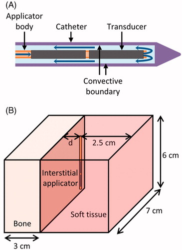
Catheter-cooled ultrasound applicators consisted of an array of two cylindrical transducers, each 1.5 mm outer diameter (OD) and 10 mm long (L), sonicating at 6.9–7.5 MHz from within a plastic implant catheter (2.4 mm OD, 1.89 mm inner diameter (ID)) with integrated water-cooling (Figure 1A). The acoustic power deposition (W/m³) from these cylindrical radiators can be described as a longitudinally collimated and radially diverging intensity pattern (I) [43,44]. where is the ultrasound absorption coefficient (Np/m), is the acoustic intensity on the transducer surface (W/m²), is the transducer radius (m), is the radial distance from the transducer’s central axis (m), and is the ultrasound attenuation coefficient (Np/m). The absorption coefficient is assumed to be equivalent to the attenuation coefficient, with scattered energy locally absorbed. The attenuation of the catheter wall was modelled as 43.9 Np/m/MHz [45].

Figure 1. (A) Diagram of the ultrasound applicators modelled. Blue arrows indicate the direction of cooling flow, which runs through the centre of the applicator, out the tip, and then between the applicator and the catheter. Transducers have an outer diameter of 1.5 mm. The catheter has an outer diameter of 2.4 mm and an inner diameter of 1.89 mm. A convective boundary condition is applied to the inner wall of the catheter. (B) Geometry used to model interstitial ultrasound ablation with the applicator at various distances (0.5 cm < d < 3.2 cm) from the surface of a flat bone.

Finite element analysis was performed using COMSOL Multiphysics 4.3 with MATLAB to generate transient temperature and thermal dose distributions for various model configurations and to model experimental studies within ex vivo tissues and phantoms. Simulations were performed on an Intel Xeon X5680 processor, with six cores each operating at 3.33 GHz on a Rad Hat Linux operating system. The catheter was modelled as a 1.89 mm ID and 2.4 mm OD cylinder, with a maximum mesh size of 0.4 mm on its inner surface. The ultrasound source was modelled as two cylinders (1.5 mm OD, 1 cm L) within the catheter. The maximum mesh size on the outermost boundaries of the geometry was 5 mm, and the maximum mesh size on heated bone surfaces was 0.3–1 mm, with finer bone meshes used when the applicator was closer to the bone surface. The mesh size in the soft tissue between the applicator and the bone was limited to a maximum of 0.7–2.5 mm, depending on the distance between the catheter and bone surfaces. Convergence tests were performed to ensure that all mesh sizes on the bone, near the applicator, and on outer boundaries were sufficiently fine for a stable solution. The initial temperature was set to 22° or 37 °C, depending on whether the simulation was performed to model bench top or physiological conditions. An implicit transient solver with a variable time step taken at least once in each 10-s time span was used to solve the transient bioheat equation. The maximum step size for thermal dose calculations was 10-20 seconds. Fixed temperature boundary conditions (equal to the initial temperature) were applied at the outermost boundaries of the geometry. A convective boundary condition was imposed on the inner surface of the catheter, with a heat transfer coefficient h = 1000 W/m²/°C [46,47] and flow temperature =22 °C. where is the normal unit vector to the boundary.

Interactions at bone/soft tissue interfaces

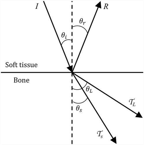
When an acoustic wave travelling through soft tissue hits a cortical bone surface, a significant portion of the energy is reflected due to an impedance mismatch. At normal incidence, the remaining energy is transmitted as longitudinal waves. If the incident angle is not normal, some or all of the transmitted energy is converted to shear waves, and both longitudinal and shear waves are refracted (Figure 2). Defining as the angle between the direction in which the wave travels and the normal of the bone surface, the reflection and refraction angles can be defined by Snell’s Law, with the reflection and transmission coefficients defined [48] as where is the reflection coefficient, is the transmission coefficient, is intensity (W/m²), is the speed of sound (m/s), subscript 1 refers to soft tissue, subscript 2 refers to bone, subscript i refers to the incident wave, subscript r refers to the reflected wave, subscript L refers to the longitudinal wave in bone, and subscript s refers to the shear wave in bone.

Figure 2. Ultrasound reflection and refraction at bone/soft tissue interfaces, as used to derive the models herein. An incident wave strikes the bone surface at angle and intensity I. The reflected wave, refracted longitudinal wave, and refracted shear wave have intensities R, T_L, and T_S and travel at angles , , and , respectively.

In contrast, specular reflection and transmission cannot be assumed in cases when cancellous bone is in direct contact with an osteolytic tumour without a smooth cortical shell in between the bone surface and the transducer. The incidence angle on the sponge-like bony trabeculae within cancellous bone is different from the incidence angle on the bulk tissue as a whole. Thus, we assume that 10% of the energy incident on cancellous bone is reflected and 90% is transmitted and locally absorbed, regardless of incidence angle [49,50].

In order to determine what approximations can accurately represent interstitial ultrasound heating at a bone/soft tissue interface, a series of models of decreasing complexity were developed (summarised in Table II). These simplified models were devised to investigate the relative impacts of reflection, refraction, mode conversion, and heating throughout the bone volume on predicted temperatures and thermal lesion sizes.

Table II. Properties of the four types of models.

Model	A: Angle-dependent volumetric	B: Constant transmission volumetric	C: Angle dependent boundary	D: Constant transmission boundary
Bone heat source	Volume	Volume	Surface	Surface
Transmission coefficient	Angle-dependent	Constant	Angle-dependent	Constant
Shear mode conversion	Yes	No	Yes	No
Reflection	Yes	No	No	No
Refraction	Yes	No	No	No

Model A: angle-dependent volumetric

The angle-dependent volumetric model, model A, considers reflection, refraction, and shear mode conversion at cortical bone interfaces. To describe heating within and adjacent to the bone, the equations describing acoustic power deposition were multiplied by the appropriate transmission and reflection coefficients, as in Moros et al. and Lin et al. [34,35]: where is the distance the reflected wave travels through soft tissue from the surface of the transducer and is the radial distance from the transducer centre to the point where the wave crosses the bone surface. , the heat deposition in soft tissue in model A, contains contributions from the incident and reflected waves. , the heat deposition in bone in model A, contains contributions from the longitudinal and shear waves. This approximation directly calculates the acoustic intensity within bone, without the need to evaluate the full stress tensor.

Model B: constant transmission volumetric

In model B, the constant transmission volumetric model, a constant attenuation coefficient and a constant transmission coefficient, both independent of incident angle, were used in bone. Reflection and refraction were not considered. Transmitted energy is assumed to be absorbed so close to the bone surface that refraction has little effect, and the heating contributions of reflected energy are assumed to be insignificant compared to heating from the incident and transmitted waves within the highly absorbing bone. The transmission coefficient () is calculated for normal incidence on a composite bone.

Model C: angle-dependent boundary and model D: constant transmission boundary

Models C and D are based upon similar equations as models A and B, respectively, but instead of volumetric power deposition within bone, all energy is assumed to be absorbed at the bone surface without penetration into the bone. Bone heating is modelled as an energy () applied to the bone surface as a power flux (W/m²) equal to the intensity on the bone surface multiplied by a transmission coefficient. The assumption is that all transmitted energy (shear and longitudinal) is absorbed within such close proximity of the bone surface that the energy may be approximated as absorbed on the bone surface. Reflection was not considered and refraction is not applicable, as this approximation assumes that the energy does not penetrate any distance into the bone. is the unit vector normal to the bone surface. The cosine terms in Equations 17 and 18 define the normal component of the energy flux through the bone surface. The transmitted angle in model D () is the same as the incidence angle ().

The transmission and reflection coefficients in the angle-dependent models, A and C, require separate shear and longitudinal components, so these two models are calculated using the acoustic properties of cortical bone. All other properties for models A–D are those of whole composite bones.

Comparison of models in perfused tissue

The four models were first compared in simulations of perfused tissues, with an initial temperature of 37 °C. The applicator was positioned in a block of muscle with its axis parallel to a flat bone and 10 or 20 mm away from it, as in Figure 1(B). A 6.9-MHz applicator was modelled, with two transducers sectored longitudinally to produce acoustic energy in a 180° angular expanse and powered at 9.4 acoustic W/cm². The initial temperature was set to 37 °C, and perfusion was considered. For each model, identical transient solvers (geometric multigrid) and meshing parameters were used.

Parametric investigations

To investigate these models and the effects of varying tumour properties, a 7-MHz applicator with a 135° active acoustic zone and two transducers was modelled in soft tissue next to a plane of composite bone, as in Figure 1(B). The largest tumour that could be ablated within 10 min for various tumour attenuation coefficients and perfusion rates was determined. The tumour attenuation was varied from 3 to 15 Np/m/MHz, representing a range of soft tissue neoplasms [27]. Tumour perfusion was varied from 0 to 13 kg/m³/s, representing zero perfusion in necrotic tumours to the high perfusion observed in some tumours [51,52]. All other tumour properties were set to those of muscle. The target was considered fully ablated when 99% of the area between the catheter and the bone surface, ranging from 1 mm below the upper transducer’s upper edge to 1 mm above the lower transducer’s lower edge, exceeded 240 CEM43 °C, which is considered a lethal thermal dose [53]. A proportional integral controller (k_p = 0.2, k_i = 0.0017) was implemented to modulate the power supplied to the transducers (limited to a range of 0–21.2 W/cm² acoustic) in order to approach and maintain a peak temperature of 85 °C. Ablations of 10 min using the constant transmission volumetric model were simulated. For low and high attenuations, models A, C, and D were also applied.

Experiments

Ex vivo tissue ablation

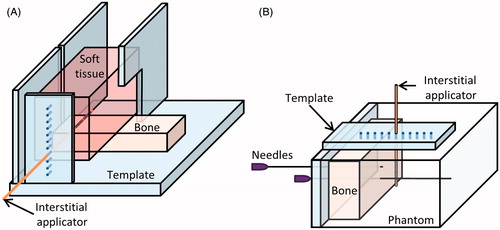
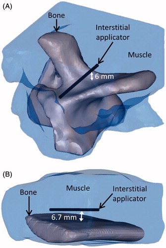
A bench-top experimental set-up, including ex vivo porcine loin muscle and bovine bones (store bought), was developed to investigate the impact of bone on thermal ablation with interstitial ultrasound (Figure 3A). Bovine rib and cervical vertebrae were cleaned of soft tissue, and the vertebrae were sectioned to produce a flat slab of cancellous bone from the centre of the vertebrae. The bones and porcine loin muscle were degassed, allowed to equilibrate to 37 °C in a water bath, and positioned adjacent to one another in a template in the bath. A catheter-cooled 6.9-MHz ultrasound applicator with two 135° transducers was inserted through the plastic template into the muscle 5–35 mm away from and parallel to an adjacent bone surface (Figure 3A). Acoustic energy (11.1, 12.5, or 22.2 W/cm²) was applied for a 10-min ablation. A total of 18 ablations incorporating rib bones and 11 ablations incorporating vertebral bones were performed, with a separate portion of the muscle and bone tissues ablated in each trial. The soft tissue was then cut through the centre of the ablation zone and the dimensions of gross tissue discoloration (coagulation) were measured.

Figure 3. Set-up of ex vivo bench-top experiments. (A) In experiments with ex vivo muscle and bone, a cut of porcine muscle was placed on top of bovine bone and heated. (B) In phantom and ex vivo bone experiments, the temperature rise in a phantom with an encapsulated bone was measured by thermocouples within needles.

Simulations of three trials with the tissue heated at 12.5 acoustic W/cm² were performed using models A–D, the geometry of Figure 1(B), and parameters mimicking the experimental conditions with the applicator positioned 15, 20, and 32 mm away from the bone. The simulated size and shape of thermal lesions, defined as cross-sectional area of the 52 °C contour [54], were compared to the measured lesions described above.

Phantom studies with invasive thermometry

To quantify the temperatures attained during interstitial ultrasound ablation involving bone, experiments were performed in soft tissue equivalent gel phantoms with embedded bones. Store bought bovine rib (representing cortical bone) and bovine cervical vertebrae were boiled and cleaned of soft tissue. The vertebrae were sectioned to produce a flat slab of cancellous bone, and then all bones were degassed under a vacuum. Two 22 gauge needles were inserted into holes predrilled through the bones, holding them with their flat surfaces upright. A tissue-mimicking phantom [55] designed for ultrasound ablation, with stable acoustic and thermal properties, was poured around the bones and allowed to solidify. A multi-junction thermocouple (five junctions, spaced every 5 mm) was placed inside one of the needles to measure the temperature in the phantom and the bone. An interstitial ultrasound applicator (6.9–7.3 MHz, 135°) within a catheter was inserted through a template into the phantom 30 mm in front of the bone, with the centre of one transducer adjacent to the thermocouple (Figure 3B). At 10 min into the heating, the thermocouple was repositioned in increments within the needle to 6–8 locations to record a detailed temperature profile at up to 40 points spaced 0–5 mm apart. After the phantom cooled to ambient temperatures, the process was repeated to measure temperature profiles with the centre of the applicator 25, 20, 15, 10, and 5 mm from the bone surface, in that order. Temperature profiles at each applicator location were obtained in three to four phantoms with an embedded rib bone and three to four phantoms with an embedded vertebral bone, for 40 ablation experiments in total.

The heating of the phantoms was simulated using the geometry in Figure 1(B), with sonication of 135° active sectors at 6.9 MHz and 16.6 acoustic W/cm². The ribs were modelled as composite bone, and the cervical bones as cancellous bone. Simulated and experimental temperature profiles were compared.

MR temperature imaging: ex vivo bone and soft tissue

Bovine rib and vertebrae with surrounding soft tissues (n = 2) were heated with interstitial ultrasound and monitored with MR temperature imaging. The ex vivo tissues, previously degassed and equilibrated to room temperature, were placed inside a birdcage transmit/receive head coil in a 3 T MR scanner (GE Healthcare, Waukesha, WI). A 7.45-MHz MR-compatible interstitial ultrasound applicator with 180° active acoustic sectors was inserted into muscle, 5–10 mm from the irregular cortical bone surfaces, with the active sectors facing the bones. The tissues were heated with applied power levels of 9.1–10.2 acoustic W/cm² for 10 min. MRTI was performed during heating, using a 2D fast spoiled gradient echo sequence with TE = 8 ms, TR = 120 ms, flip angle = 30°, rib field of view = 12 × 12 cm², and vertebra field of view = 14 × 14 cm² in eight slices that were 5 mm thick and perpendicular to the applicator axis. The shift in the proton resonance frequency (PRF) of water, via phase mapping, was used to calculate temperature [56]. As commonly applied with this approach, phase unwrapping of the complex MR signal was performed to correct jumps in the phase changes from −π to π [57].

Three-dimensional models of the ex vivo rib and vertebrae ablations monitored with MRTI were developed. The Mimics Innovation Suite (Materialise NV, Leuven, Belguim) was used to manually segment MR images acquired before each ablation and to create finite element method (FEM) meshes specific to the tissue geometry. To create FEM meshes, the segmented 3D images were converted to 3D objects represented by triangular surface meshes and smoothed. A cylinder with a diameter of 1.89 mm was added to the geometry to represent the cooled inner surface of the catheter. All the surface meshes were refined to be within the size ranges used in this study (0.3–5 mm, with finer meshes where more acoustic energy is deposited), and combined into a single surface mesh of the volume. The surface mesh was then converted to a volume mesh and imported into Comsol.

The spatial distribution of heat deposition in tissue () was calculated in MATLAB and imported into Comsol. First, the ultrasound attenuation coefficients throughout the volume, as defined in Comsol, were imported into MATLAB. MATLAB was then used to integrate the acoustic attenuation over a fine spatial resolution, calculate the transmission coefficients, and determine the acoustic heat deposition on the finite element grid. In contrast, heat deposition in volumes composed of rectangular prisms to model tissue and cylinders to model ultrasound applicators (Figure 1B) was calculated analytically within Comsol. Meshes representing such volumes were also developed within Comsol. Because tissue surfaces relatively close to the heated region were exposed to air in the cases monitored with MRTI, a heat flux with h = 10.5 W/m/°C [58,59] and =22 °C was used on the outer boundaries. Due to the complexity of tracing the paths of reflected and refracted rays through the irregular geometries of bone/muscle interfaces as required for model A, these two cases were modelled using models B–D.

Results

Theory

Comparison of models in perfused tissue

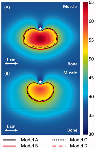
Figure 4 shows the temperature maps predicted by model B, and compares the 240 CEM43 °C contours, which correspond to ablated regions, for the four models when the applicator is placed in perfused muscle at 1 and 2 cm from a flat bone surface. The approximations in models B and D produced thermal dose contours that closely matched the more comprehensive model A. However, when the applicator was close enough to ablate the bone surface, model C produced 240 CEM43 °C contours that did not extend as deeply (5.0 mm) into the bones as the other three (5.3–5.8 mm). The boundary models (C and D) had significantly shorter computation times than the volumetric models (A and B). Model D was solved 3.6, 2.6, and 1.5 times faster than models A, B, and C, respectively, when the applicator was 1 cm from bone. It took 218, 156, 89, and 60 min, respectively, to compute 10-min transient simulations using models A-D on an Intel Xeon X5680 processor. In these cases, models C and D had a mesh size of 0.8 mm on the heated portion of the bone surface and 332,741 elements total, while models A and B, which required a finer bone mesh, had a mesh size of 0.5 mm on heated bone surfaces and 540,505 elements total.

Figure 4. 240 CEM43 °C contours calculated with models A–D after a 10-min ablation are shown in the central plane between the two transducers. The applicators (white circle) are placed 1 and 2 cm from a flat bone (black line) in A and B, respectively. A colour map shows the temperatures (°C) calculated with the constant transmission volumetric model (model B).

Parametric investigations

A parametric study was performed to investigate the influence of attenuation and perfusion on the volume of tissue that could be ablated in the presence of bone and to determine how the models perform in tissues with various properties. The maximum distance between the applicator and a flat bone at which all tissue between the two could be ablated is shown in Figure 5 for various soft tissue perfusions and attenuations. The maximum tumour size that could be ablated with zero and maximum perfusion in soft tissue without bone present is also shown.

Figure 5. The maximum distance between an applicator and a flat bone at which all tumour tissue between the two can be ablated within 10 min, given various ultrasound attenuations and blood perfusion rates in the tumour, as calculated by model B. The maximum radius that can be fully ablated when bone is absent is also shown for 0 and 13 kg/m³/s perfusion in the tumour. The maximum distance between an applicator and bone for which all intervening tissue can be ablated is also plotted for models A (+), C (o), and D (Δ) for attenuations of 4 and 12.5 Np/m/MHz and perfusions of 0 (black), 5 (red), and 13 (blue) kg/m³/s.

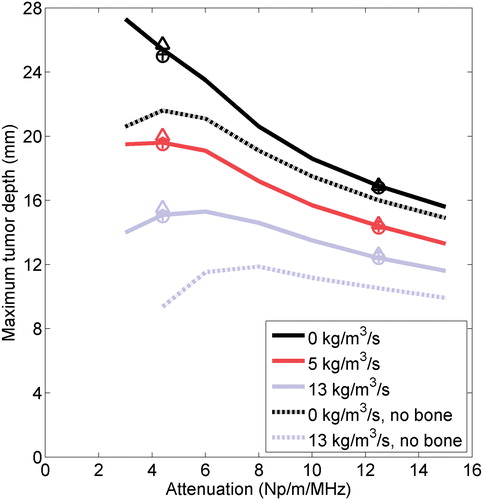
Significantly larger tumours could be ablated when bone was present at the outer boundary, especially when the tumour attenuation was low. The largest tumours that could be ablated with bone present had low attenuations and perfusions, though there was a fall-off in the volume that could be ablated at the lowest attenuations. At 13 kg/m³/s and exceptionally low attenuation (3 Np/m/MHz), the combined effects of perfusion, low absorption, and catheter cooling for the parameters tested herein resulted in reduced heating in the tissue immediately adjacent to the applicator, so it could not be ablated within 10 min at the maximum allowable power unless bone was present. In practice, the cooling flow could be applied at a higher temperature or turned off immediately after power application to effectively coagulate tissue adjacent to the applicator. The four models agreed well on the radii of the ablated volumes, regardless of the tumour attenuation or perfusion, with better agreement at high attenuations. The discrepancy between the calculations made by model A and the calculations made by the other models of the maximum distance between the bone and applicator at which all intervening tissue could be ablated was less than 2.6% for all cases evaluated.

Experiments

Thermal lesions: ex vivo bone and tissue studies

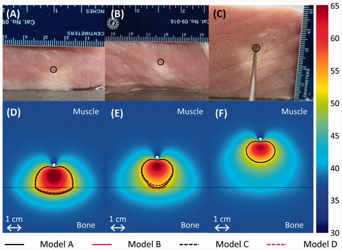
Porcine muscle was ablated using interstitial ultrasound in a 37 °C water bath, with the applicator positioned various distances from flat slabs of cortical and cancellous bone. Models A–D predicted coagulated regions of similar sizes and shapes as those produced experimentally (Figure 6). Model C tended to slightly underestimate the size of thermal lesions compared to the other models. The measurement of the distance between the applicator and the bone recorded after the ablation was consistently lower, particularly at higher powers, than the measurement from before the ablation by an average of 2.3 mm, which is attributed to tissue shrinkage during coagulation [60].

Figure 6. (A–C) Thermal lesions created by 10-min ablations at 12.5 acoustic W/cm² in porcine muscle positioned directly atop bovine bone, shown in central cross-sections through the lesions. The catheter was measured as 15.2, 19.7, and 32.3 mm away from the bone before heating in A–C respectively, and 11.5, 17, and 32 mm away from the bone after the experiment. The catheter track is circled, and the side of the tissue that was against the bone is shown against the table. In C, a metal rod illustrates the catheter position. (D–F) The experiments were modelled with the applicator 15, 20, and 32 mm away from the bone, respectively, and the results after a 10-min ablation are plotted in the central plane between the two transducers. The resulting temperature profiles produced by model A are shown in a colour map (°C). A black line indicates the bone/muscle boundary, and curves outline the 52 °C temperature contours for models A–D.

Thermometry: ex vivo bone and phantom studies

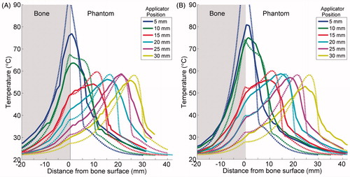
Figure 7 shows a series of temperature profiles measured in one phantom containing a rib bone (A) and another phantom containing cancellous bone (B) after 10-min ablations by applicators positioned 5–30 mm from the bone/phantom interface. The temperatures were measured by thermocouples along a line running through the bone, into the phantom, and alongside one transducer (Figure 3B). The experiments were modelled, and the theoretical results created using the constant transmission volumetric model (model B) are superimposed in Figure 7. The temperature peaked near the applicator, and a secondary peak or inflection was observed at the bone surface, behind which the temperature would sharply drop off. When the bone was within 1 cm of the applicator, the primary and secondary peaks overlapped, producing a single, higher temperature peak. The simulated models A–D demonstrated all of these trends in temperature.

Figure 7. Experimental (---) and simulated (– – –) temperature profiles after 10-min ablations in two phantoms containing cortical (A) or cancellous (B) bone. Temperature along a line perpendicular to the bone surface and adjacent to the centre of one transducer, as in Figure 3(B), is plotted as a function of distance from the bone surface, which is at x = 0. Positive x-values are in the phantom, and negative values are inside the bone. Each solid curve corresponds to a single experimental trial with the applicator placed at the designated distance from the bone. The experiments were simulated with model B, and the theoretical results are superimposed as dashed lines.

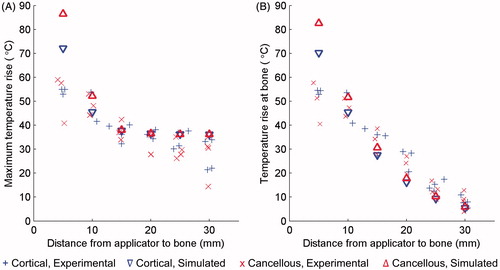
The maximum temperature rises recorded after a 10-min ablation are plotted against the distance between the applicator and the bone surface for each of the 40 trials in Figure 8(A), with simulated data superimposed. Figure 8(B) shows the recorded and simulated temperature rises at the bone surface for each trial. The maximum temperature achieved tends to be constant with respect to applicator location until the applicator is within 1 cm from the bone, at which point the primary and secondary temperature peaks overlap, and the maximum temperature increases sharply. Overall, the simulations predicted the maximum temperatures fairly accurately and reproduced the same trends as experiments. Some deviations between the two were observed, in that the simulations underestimated bone surface temperatures when the applicator was 15 mm or more from the bone, and over-predicted bone surface temperatures when the applicator was 5 mm from the bone.

Figure 8. The maximum temperature increase measured at the end of each 10-min ablation of a phantom with an embedded bone is plotted in A. The temperature increase at the bone surface at the end of each trial is plotted in B. Peak (A) and bone (B) temperature increases produced by simulations using the constant transmission longitudinal model (model B) are superimposed.

Figure 9 shows the mean measured temperature profiles from experiments compared to simulated temperature profiles corresponding to each of the four models, for two example cases with the applicator 10 and 25 mm from cortical bone. Good agreement was observed between the experimental temperature profiles and simulations with models A–D for all six distances between the applicator and the bone, with correlation coefficients ranging between 0.852 to 0.967 (Table III). The maximum p-value, based on a t-statistic, was 1.9 e-31. The correlation coefficients between model A and models B–D were at least 0.995 for all six applicator locations, with maximum p-values, based on a t-statistic, of zero.

Figure 9. Simulated and experimental temperature profiles in phantoms with an applicator placed 10 mm (A) and 25 mm (B) from a rib surface. Temperature along a line perpendicular to the bone surface and adjacent to the centre of one transducer, as in Figure 3(B), is plotted as a function of distance from the bone surface, which is at x = 0. Recordings were made after 10 min of heating. The experimental curve is an average of the recordings in three to four experiments with the applicator at the given position. The bone surface is at x = 0. Positive x-values indicate locations in the phantom, and negative values are inside the bone.

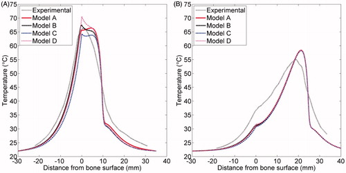
Table III. Correlation coefficients between experimental and simulated temperature profiles in phantoms.

Distance between applicator and bone (mm)	30	25	20	15	10	5
Model A	0.854	0.893	0.886	0.901	0.955	0.967
Model B	0.853	0.892	0.888	0.908	0.960	0.958
Model C	0.852	0.890	0.878	0.889	0.944	0.961
Model D	0.853	0.893	0.890	0.907	0.955	0.958

The correlation coefficients between each of the four models A–D and the temperature measurements recorded at all thermocouple locations in 3–4 phantoms after a 10-min ablation were calculated for each of the six applicator positions. The maximum p-value, based on a t-statistic, was 1.9e-31.

MR temperature imaging

The FEM meshes created based on segmented MR images captured the applicator position and the complex geometry of the soft tissues, bovine rib, and bovine vertebrae heated under MRTI monitoring (Figure 10). Parametric studies with complex geometries based on segmented MR images as well as simple geometries based on the phantom set-up indicated that a 0.3–1 mm mesh was necessary on heated portions of the bone surface when using models A and B, depending on the distance between the applicator and the bone, while a 0.8–1 mm mesh on heated bone surfaces was sufficient for models C and D. The total mesh sizes and computation times for the rib models were 413,000 elements and 47 min for model B, and 350,000 elements and 32–36 min for models C and D. For the vertebra case, the simulations performed with model B had 802,000 elements and took 85 min, while simulations using models C and D had 428,000 elements and both took 49 min. These 10-min transient simulations were performed on an Intel Xeon X5680 processor.

Figure 10. 3D objects that were meshed to model the bovine vertebra (A) and bovine rib (B) ablations monitored by MR thermometry.

Figures 11–12 show the recorded temperature increases and simulated temperature contours 5 min into the ablation, when all soft tissue between the applicator and the bone was heated at least 15 °C, which is ablative under in vivo conditions [54]. The predictions of the temperatures, as well as the shapes and sizes of the isothermal contours, produced by models B and D were in close agreement with MRTI. Model C produced the smallest contoured areas, and model B produced the largest. In the muscle surrounding the vertebrae in a 24 × 33 × 30 mm region around the transducers, the temperatures produced after a 10-min ablation by model B had an error of 0.1° ± 4.0 °C (mean ± standard deviation), model C had an error of −1.2° ± 3.8°C, and model D had an error of −0.1° ± 3.9 °C when compared to experimental measurements. In the muscle surrounding the rib in a 24 × 37 × 30 mm region around the transducers, the temperatures produced by model B had an error of −1.3° ± 3.9 °C (mean ± standard deviation), model C had an error of −2.3° ± 3.8 °C, and model D had an error of −1.4° ± 3.8 °C as compared to experimental measurements. The deviation of the models from experimental values was less significant at earlier time points. The models under-predicted the mild temperature rises experimentally observed behind the applicator, which is not heated by incident ultrasound energy, with errors less than or equal to the errors in the zone of maximal heating. Generally, lower errors in simulated temperatures were observed in the periphery, away from the zone of maximal heating. Tissue heterogeneity and the limitations of the slice thickness in MR images could possibly contribute to these errors.

Figure 11. (A–C) MR images of the three central heated axial slices of ex vivo bovine vertebrae, spaced 5 mm apart. (D–F) Colour map of temperature increases (°C) recorded with MRTI in a smaller field of view (magenta box) for each slice 5 min into the ablation. Bone is outlined with a white line, and the 20 °C temperature increase contours recorded by MRTI are outlined in black. Also shown are the simulated 20 °C temperature increase contours produced by models B (magenta), C (grey), and D (blue).

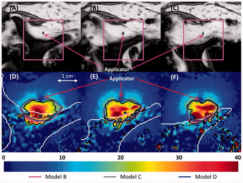
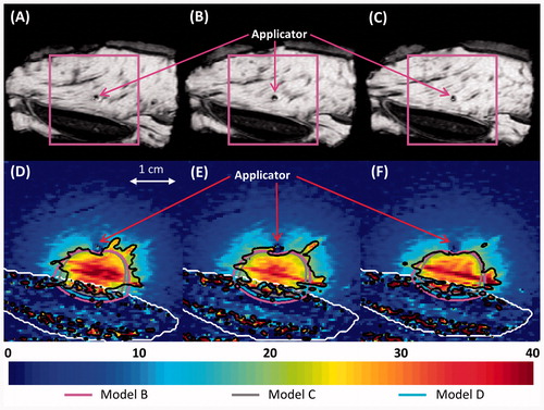
Figure 12. (A–C) MR images of the three central heated axial slices of ex vivo bovine rib, spaced 5 mm apart. (D–F) Colour map of temperature increases (°C) recorded with MRTI is shown in a smaller field of view (magenta box) for each slice 5 min into the ablation. Bone is outlined with a white line, and the 20 °C temperature increase contours recorded by MRTI are outlined in black. Also shown are the 20 °C temperature increase contours produced by models B (magenta), C (grey), and D (cyan).

Discussion

The presence of bone within or adjacent to a target region can dramatically influence the heating characteristics of ultrasound therapy in general, and specifically interstitial ultrasound as addressed in this study. Bone interfaces are complicated by two distinct parameters: high acoustic absorption of bone and high acoustic impedance differences. Bone has an ultrasound absorption coefficient one to two orders of magnitude higher than that of soft tissue [27], causing preferential heating at the bone surface [25,28], effectively creating a secondary heat source and insulating structures behind the bone (Figures 6 and 7). Acoustic impedance differences between bone and soft tissue result in reflection, refraction, and mode conversion at the interface, which complicate wave propagation and prediction of resultant heating patterns. Complex accurate acoustic modelling of this interface is computationally intensive and difficult, especially considering that the stress tensor in solids cannot be simplified as a one dimensional pressure as it can be in liquids. In this work we have devised approximate models of the interactions of interstitial ultrasound with bone. Theoretical and comparative experimental studies with bone/tissue phantoms and ex vivo tissues have demonstrated that these simplifications can provide accurate estimations of temperature distributions with reduced modelling complexity and computational requirements, and that they are practical for applications in treatment planning and modelling.

Models using four methods (A–D) of decreasing complexity to calculate heat deposition in bone were developed and compared. Models B and D produced temperature and thermal dose distributions very similar to the more comprehensive model A (Figures 4–6, 9), demonstrating that neither angle-dependent nor volumetric heat sources are crucial to modelling high-frequency interstitial ultrasound heating in bone. Any discrepancies between the four models generally occurred near the most heated portions of the bone surface (Figures 4 and 9) and were lower at earlier time points. Model A, which included reflection, produced slightly higher temperatures in volumes of the soft tissue that are not heated by incident ultrasound energy than the other models (Figure 9). At 7 MHz, 69% (longitudinal) to 83% (shear) of the acoustic energy entering bone is attenuated and absorbed within 1 mm, and 97% (longitudinal) to 99.5% (shear) is absorbed within 3 mm. Shear and longitudinal penetration beyond 3 mm is negligible. Unless the bone is very thin, the amount of energy that exits the bone to propagate through soft tissue, which is further decreased by the transmission coefficient, is negligible and does not need to be modelled. The high attenuation coefficient of bone allows for so little acoustic penetration that the different pathways of shear and longitudinal waves do not need to be modelled separately, and heating can be approximated as occurring on the face of the bone surface.

The angle-dependent boundary model (C), however, consistently produced temperature distributions that were lower overall than the three other models and MRTI data (Figures 4, 6, 9, 11, 12). In regions with measured temperature increases over 15 °C, model C produced temperature increases 3.1 ± 3.5% (mean ± standard deviation) below those of model A in phantoms and 6.9 ± 13.2% below those of thermocouple measurements in phantoms. The low heating observed in model C may have resulted from the use of lower transmission and attenuation coefficients near normal incidence than models B and D, as well as from neglecting the heat generated by reflected waves. When constant transmission coefficients are used (models B and D), the lack of reflected energy resulted in only a slight decrease in soft tissue temperatures as compared to model A (Figure 9).

Although model D included the most approximations, it performed very well. Model D approximated model A (the most comprehensive model) more closely than models B and C did in almost all locations over a few mm away from the bone/phantom interface when the applicator was 1–3 cm away from it (Figure 9). The RMS (root mean square) errors in models A–C, as compared to experimentally measured values in regions heated at least 5 °C in phantoms, were each within 0.5 °C of the RMS error of model D. Also, model D was much better than model C and just slightly worse than model B in estimating temperature measurements made by MRTI, with the applicator 5–10 mm from the bone surfaces.

Models A, B, and D are all suitable for simulating interstitial ultrasound ablation involving bone. The volumetric models A and B, however, can require a much finer mesh size (0.3–1 mm) at the bone surface than the surface models C and D (0.8–1 mm), possibly because they may need a fine resolution to capture the rapid fall-off in acoustic intensity behind the bone surface. This greatly increases computational time, particularly when the bone has a high surface area. A is also difficult to model in complex geometries, as the paths of reflected and refracted beams must be traced. Although development of a fast modelling platform is not a primary goal of this study, the impact of model approximations on computation time was analysed in consideration of potential future treatment planning applications. Since models A, B, and D yield similar temperature predictions, the simplest and fastest one would be best suited to treatment planning. As such, model D may be the most practical method for accurately simulating interstitial ultrasound bone ablation, with model B preferable in cases when the bone is less than 1–2 mm thick.

Simulations produced temperature profiles and ablated volumes that closely matched experimental data in size and shape (Figures 6–9, 11, 12). Simulated temperatures were very close to data measured with thermocouples and MRTI. The one exception was the over-prediction of peak temperatures in phantoms when the applicator was 5 mm from the bone surface. Thermocouple conduction artefacts, which smear heating along the multi-junction thermocouple wires, may have contributed to this discrepancy [61]. This artefact would be more pronounced when a large amount of heat is deposited in a small region, as in the 5-mm phantom case, lowering the measured temperatures below the actual temperatures. The predicted temperatures at the phantom/bone interface when the applicator was 10 mm or more away from the bone were generally within the range of experimental values (Figure 8). Figures 6–9, 11, and 12 show fairly good agreement of temperature and thermal dose profiles between the models and the experiments in the zones of maximal heating at the end of treatment. Discrepancies between the models and experiments were generally even smaller at earlier time points and in locations away from the zones of maximal heating.

The results of this study demonstrate the importance of modelling the interactions of interstitial ultrasound with bone, as preferential bone heating can dramatically impact heating and thermal dose profiles. Simulations and temperature measurements in phantoms indicate that when an applicator is within 1 cm of the bone surface, the temperature peaks at the bone surface and in the soft tissue overlap, creating a high, narrow peak near the bone surface (Figure 7). When the applicator is further from the bone, the secondary peak at the bone surface can widen the ablated region without significantly changing peak temperatures (Figures 7–8). This effect is more pronounced at low attenuations and perfusions, when ultrasound can penetrate further into the tumour to reach the bone and less of the absorbed energy is carried away by flowing blood (Figure 5). These results agree with those of Moros et al., who performed similar experiments using phantoms with bone inclusions and an external planar transducer to study hyperthermia at 1.0 and 3.3 MHz in superficial tissues above bone [62]. They found that increased heating near the bone surface can be significant, and can be used to enhance acoustic and thermal penetration into deep tissue regions directly over bone. These studies also corroborated extensive theoretical investigations [34,37], which were employed in part for the development of our models herein.

Comparison with MRTI data shows that the simulations of irregularly shaped bones produced fairly accurate biothermal and acoustic models. MRI is highly useful for its ability to monitor heating and to create images on which 3D models for treatment planning can be based. MRTI measured temperature rises in the soft tissue adjacent to bone. MRTI data within bone measured with the PRF method is inaccurate because cortical bone has low water content and thus a low MR signal, because cancellous bone has a high fat content, and because fat suppression was not applied. Future applications may be able to use fat suppression or data in adjacent soft tissues to infer or predict bone temperatures. The system developed here for modelling interstitial ultrasound ablation involving bone could potentially be used to plan and monitor treatments in complex osseous anatomy such as the spine.

Conclusion

Models and experimental data showed that preferential heating at bone surfaces can cause higher temperature elevations or allow larger volumes to be ablated with interstitial ultrasound. Four types of biothermal and acoustic models of interstitial ultrasound ablation involving bone were developed, applying various approximations, and compared to experimental data. Three of the models produced temperature and thermal dose profiles very similar to those observed experimentally. Approximations that considered a constant transmission coefficient, heat sources applied to the bone/soft tissue boundary, no reflection, and no shear mode conversion represented heating in bone and soft tissues with good accuracy, while simplifying and speeding up simulations. Models generated for case-specific anatomy, incorporating finite element meshes representing the precise geometry of the tissues heated, made fairly accurate temperature predictions, as evidenced by favourable comparison with MRTI data. Modelling techniques developed here can be applied to treatment planning and optimisation in a wide variety of tumours near or adjacent to bone.

Declaration of interest

We gratefully acknowledge support by the National Institutes of Health (NIH) grant R44CA112852. This work is a collaboration between the University of California at San Francisco and Acoustic MedSystems supported by a Small Business Industry Research grant from the NIH. Clif Burdette is affiliated with Acoustic MedSystems, Inc., which has a commercial interest in interstitial ultrasound technology. The authors alone are responsible for the content and writing of the paper.

References

- Coleman R. Metastatic bone disease: Clinical features, pathophysiology and treatment strategies. Cancer Treat Rev 2001;27:165–76
- Mundy GR. Metastasis to bone: Causes, consequences and therapeutic opportunities. Nat Rev Cancer 2002;2:584–93
- SEER Cancer Statistics Review, 1975–2009 (Vintage 2009 populations). In: Howlander N, Noone AM, Krapcho M, Neyman N, Aminou R, Altekruse SF, et al., eds. Bethesda, MD: National Cancer Institute, 2012
- Klimo P Jr, Schmidt MH. Surgical management of spinal metastases. Oncologist 2004;9:188–96
- Callstrom MR, Charboneau JW, Goetz MP, Rubin J, Atwell TD, Farrell MA, et al. Image-guided ablation of painful metastatic bone tumors: A new and effective approach to a difficult problem. Skeletal Radiol 2006;35:1–15
- Georgy BA. Metastatic spinal lesions: State-of-the-art treatment options and future trends. Am J Neuroradiol 2008;29:1605–11
- Healey JH, Brown HK. Complications of bone metastases. Cancer 2000;88:2940–51
- Schwab JH, Springfield DS, Raskin KA, Mankin HJ, Hornicek FJ. What’s new in primary bone tumors. J Bone Joint Surg Am 2012;94:1913–9
- Rosenthal D, Callstrom MR. Critical review and state of the art in interventional oncology: Benign and metastatic disease involving bone. Radiology 2012;262:765–80
- Pinto CH, Taminiau AHM, Vanderschueren1 GM, Hogendoorn PCW, Bloem JL, Obermann WR. Technical considerations in CT-guided radiofrequency thermal ablation of osteoid osteoma: Tricks of the trade. Am J Roentgenol 2002;179:1633–42
- Tins B, Cassar-Pullicino V, McCall I, Cool P, Williams D, Mangham D. Radiofrequency ablation of chondroblastoma using a multi-tined expandable electrode system: Initial results. Eur Radiol 2006;16:804–10
- Schaefer O, Lohrmann C, Markmiller M, Uhrmeister P, Langer M. Combined treatment of a spinal metastasis with radiofrequency heat ablation and vertebroplasty. Am J Roentgenol 2003;180:1075–7
- Nakatsuka A, Yamakado K, Maeda M, Yasuda M, Akeboshi M, Takaki H, et al. Radiofrequency ablation combined with bone cement injection for the treatment of bone malignancies. J Vasc Interv Radiol 2004;15:707–12
- Liberman B, Gianfelice D, Inbar Y, Beck A, Rabin T, Shabshin N, et al. Pain palliation in patients with bone metastases using MR-guided focused ultrasound surgery: A multicenter study. Ann Surg Oncol 2009;16:140–6
- Catane R, Beck A, Inbar Y, Rabin R, Shabshin N, Hengst S, et al. MR-guided focused ultrasound surgery (MRgFUS) for the palliation of pain in patients with bone metastases – Preliminary clinical experience. Ann Oncol 2007;18:163–7
- Gianfelice D, Gupta C, Kucharczyk W, Bret P, Havill D, Clemons M. Palliative treatment of painful bone metastases with MR imaging-guided focused ultrasound. Radiology 2008;249:355–63
- Simon CJ, Dupuy DE, Mayo-Smith WW. Microwave ablation: Principles and applications. Radiographics 2005;25:S69–83
- Gangi A, Dietemann J, Gasser B, Mortazavi R, Brunner P, Mourou M, et al. Interstitial laser photocoagulation of osteoid osteomas with use of CT guidance. Radiology 1997;203:843–8
- Callstrom MR, Atwell TD, Charboneau JW, Farrell MA, Goetz MP, Rubin J, et al. Painful metastases involving bone: Percutaneous image-guided cryoablation – Prospective trial interim analysis. Radiology 2006;241:572–80
- Diederich CJ. Ultrasound applicators with integrated catheter-cooling for interstitial hyperthermia: Theory and preliminary experiments. Int J Hyperthermia 1996;12:279–97
- Nau WH, Diederich CJ, Burdette EC. Evaluation of multielement catheter-cooled interstitial ultrasound applicators for high-temperature thermal therapy. Med Phys 2001;28:1525–34
- Lafon C, Melodelima D, Salomir R, Chapelon JY. Interstitial devices for minimally invasive thermal ablation by high-intensity ultrasound. Int J Hyperthermia 2007;23:153–63
- Deardorff DL, Diederich CJ, Nau WH. Control of interstitial thermal coagulation: Comparative evaluation of microwave and ultrasound applicators. Med Phys 2000;28:104–17
- Nau WH, Diederich CJ, Stauffer PR. Directional power deposition from direct-coupled and catheter-cooled interstitial ultrasound applicators. Int J Hyperthermia 2000;16:129–44
- Fujii M, Sakamoto K, Toda Y, Negishi A, Kanai H. Study of the cause of the temperature rise at the muscle–bone interface during ultrasound hyperthermia. IEEE Trans Biomed Eng 1999;46:494–504
- Chan AK, Sigelmann RA, Guy AW. Calculations of therapeutic heat generated by ultrasound in fat–muscle–bone layers. IEEE Trans Biomed Eng 1974;BME-21:280–4
- Duck F. Physical properties of tissue: A comprehensive reference book. London: Academic Press, 1990
- Hynynen K, DeYoung D. Temperature elevation at muscle–bone interface during scanned, focused ultrasound hyperthermia. Int J Hyperthermia 1988;4:267–79
- Bossy E, Padilla F, Peyrin F, Laugier P. Three-dimensional simulation of ultrasound propagation through trabecular bone structures measured by synchrotron microtomography. Phys Med Biol 2005;50:5545–56
- Kaufman JJ, Luo G, Siffert RS. Ultrasound simulation in bone. IEEE Trans Ultrason, Ferroelectr, Freq Control 2008;55:1205–18
- Behnia S, Jafari A, Ghalichi F, Bonabi A. Finite-element simulation of ultrasound brain surgery: Effects of frequency, focal pressure, and scanning path in bone-heating reduction. Cent Eur J Phys 2008;6:211–22
- Burtnyk M, Chopra R, Bronskill M. Simulation study on the heating of the surrounding anatomy during transurethral ultrasound prostate therapy: A 3D theoretical analysis of patient safety. Med Phys 2010;37:2862–75
- Wootton JH, Ross AB, Diederich CJ. Prostate thermal therapy with high intensity transurethral ultrasound: The impact of pelvic bone heating on treatment delivery. Int J Hyperthermia 2007;23:609–22
- Moros EG, Straube WL, Myerson RJ, Fan X. The impact of ultrasonic parameters on chest wall hyperthermia. Int J Hyperthermia 2000;16:523–38
- Lin W-L, Liauh C-T, Chen Y-Y, Liu H-C, Shieh M-J. Theoretical study of temperature elevation at muscle/bone interface during ultrasound hyperthermia. Med Phys 2000;27:1131–40
- Sun J, Hynynen K. Focusing of therapeutic ultrasound through a human skull: A numerical study. J Acoust Soc Am 1998;104:1705–15
- Moros EG, Fan X, Straube WL. Ultrasound power deposition model for the chest wall. Ultrasound Med Biol 1999;25:1275–87
- Wu J, Du G. Temperature elevation generated by a focused Gaussian ultrasonic beam at a tissue–bone interface. J Acoust Soc Am 1990;87:2748–55
- Lu B-Y, Yang R-S, Lin W-L, Cheng K-S, Wang C-Y, Kuo T-S. Theoretical study of convergent ultrasound hyperthermia for treating bone tumors. Med Eng Phys 2000;22:253–63
- Pennes HH. Analysis of tissue and arterial blood temperatures in the resting human forearm. J Appl Physiol 1948;1:93–122
- Prakash P, Diederich CJ. Considerations for theoretical modelling of thermal ablation with catheter-based ultrasonic sources: Implications for treatment planning, monitoring and control. Int J Hyperthermia 2012;28:69–86
- Sapareto SA, Dewey WC. Thermal dose determination in cancer therapy. Int J Radiat Oncol Biol Phys 1984;10:787–800
- Diederich CJ, Hynynen K. Induction of hyperthermia using an intracavitary multielement ultrasonic applicator. IEEE Trans Biomed Eng 1989;36:432–8
- Tyréus PD, Diederich CJ. Theoretical model of internally cooled interstitial ultrasound applicators for thermal therapy. Phys Med Biol 2002;47:1073–89
- Chen X, Diederich CJ, Wootton JH, Pouliot J, Hsu I-C. Optimisation-based thermal treatment planning for catheter-based ultrasound hyperthermia. Int J Hyperthermia 2010;26:39–55
- Wootton JH, Prakash P, Hsu I-CJ, Diederich CJ. Implant strategies for endocervical and interstitial ultrasound hyperthermia adjunct to HDR brachytherapy for the treatment of cervical cancer. Phys Med Biol 2011;56:3967
- Prakash P, Salgaonkar VA, Clif Burdette E, Diederich CJ. Multiple applicator hepatic ablation with interstitial ultrasound devices: Theoretical and experimental investigation. Med Phys 2012;39:7338–49
- Cheeke JDN. Fundamentals and Applications of Ultrasonic Waves. Boca Raton, FL: CRC Press, 2012
- Riekkinen O, Hakulinen M, Timonen M, Töyräs J, Jurvelin J. Influence of overlying soft tissues on trabecular bone acoustic measurement at various ultrasound frequencies. Ultrasound Med Biol 2006;32:1073–83
- Hakulinen MA, Day JS, Töyräs J, Timonen M, Kröger H, Weinans H, et al. Prediction of density and mechanical properties of human trabecular bone in vitro by using ultrasound transmission and backscattering measurements at 0.2–6.7 MHz frequency range. Phys Med Biol 2005;50:1629–42
- Vaupel P, Kallinowski F, Okunieff P. Blood flow, oxygen and nutrient supply, and metabolic microenvironment of human tumors: A review. Cancer Res 1989;49:6449–65
- Gerweck LE. Hyperthermia in cancer therapy: The biological basis and unresolved questions. Cancer Res 1985;45:3408–14
- Dewey WC. Arrhenius relationships from the molecule and cell to the clinic. Int J Hyperthermia 1994;10:457–83
- Kinsey AM, Diederich CJ, Rieke V, Nau WH, Butts Pauly K, Bouley D, et al. Transurethral ultrasound applicators with dynamic multi-sector control for prostate thermal therapy: In vivo evaluation under MR guidance. Med Phys 2008;35:2081–93
- King RL, Liu YL, Maruvada S, Herman BA, Wear KA, Harris GR. Development and characterization of a tissue-mimicking material for high intensity focused ultrasound. IEEE Trans Ultrason, Ferroelectr, Freq Control 2011;58:1397–405
- Rieke V, Butts Pauly K. MR thermometry. J Magn Reson Imaging 2008;27:376–90
- Roujol S, Ries M, Quesson B, Moonen C, Denis de Senneville B. Real‐time MR‐thermometry and dosimetry for interventional guidance on abdominal organs. Magn Reson Med 2010;63:1080–7
- Buccella C, De Santis V, Feliziani M. Prediction of temperature increase in human eyes due to RF sources. IEEE Trans Electromagn Compat 2007;49:825–33
- Wang J, Fujiwara O. FDTD computation of temperature rise in the human head for portable telephones. IEEE Trans Microw Theory Techn 1999;47:1528–34
- Brace CL, Diaz TA, Hinshaw JL, Lee FT. Tissue contraction caused by radiofrequency and microwave ablation: A laboratory study in liver and lung. J Vasc Interv Radiol 2010;21:1280–6
- Dickinson RJ. Thermal conduction errors of manganin-constantan thermocouple arrays. Phys Med Biol 1985;30:445
- Moros EG, Novak P, Straube WL, Kolluri P, Yablonskiy DA, Myerson RJ. Thermal contribution of compact bone to intervening tissue-like media exposed to planar ultrasound. Phys Med Biol 2004;49:869–86
- Damianou C, Sanghvi N, Fry F. Dependence of ultrasonic attenuation and absorption in dog soft tissues on temperature and thermal dose. J Acoust Soc Am 1997;102:628–34
- Werner J, Buse M. Temperature profiles with respect to inhomogeneity and geometry of the human body. J Appl Physiol 1988;65:1110–8
- Williams LR, Leggett RW. Reference values for resting blood flow to organs of man. Clin Phys Physiol Meas 1989;10:187–217
- Calttenburg R, Cohen J, Conner S, Cook N. Thermal properties of cancellous bone. J Biomed Mater Res 1975;9:169–82
- McCarthy I. The physiology of bone blood flow: A review. J Bone Joint Surg Am 2006;88:4–9
- Wu J, Cubberley F. Measurement of velocity and attenuation of shear waves in bovine compact bone using ultrasonic spectroscopy. Ultrasound Med Biol 1997;23:129–34