Cell death, perfusion and electrical parameters are critical in models of hepatic radiofrequency ablation

Abstract

Purpose: A sensitivity analysis has been performed on a mathematical model of radiofrequency ablation (RFA) in the liver. The purpose of this is to identify the most important parameters in the model, defined as those that produce the largest changes in the prediction. This is important in understanding the role of uncertainty and when comparing the model predictions to experimental data. Materials and methods: The Morris method was chosen to perform the sensitivity analysis because it is ideal for models with many parameters or that take a significant length of time to obtain solutions. A comprehensive literature review was performed to obtain ranges over which the model parameters are expected to vary, crucial input information. Results: The most important parameters in predicting the ablation zone size in our model of RFA are those representing the blood perfusion, electrical conductivity and the cell death model. The size of the 50 °C isotherm is sensitive to the electrical properties of tissue while the heat source is active, and to the thermal parameters during cooling. Conclusions: The parameter ranges chosen for the sensitivity analysis are believed to represent all that is currently known about their values in combination. The Morris method is able to compute global parameter sensitivities taking into account the interaction of all parameters, something that has not been done before. Research is needed to better understand the uncertainties in the cell death, electrical conductivity and perfusion models, but the other parameters are only of second order, providing a significant simplification.

• Cell death
• mathematical model
• radiofrequency ablation
• sensitivity analysis

Introduction

Radiofrequency ablation (RFA) is a treatment option for primary and metastatic liver cancer when surgery is not an option. It is a minimally invasive procedure involving the placement of an applicator within a target tumour under image guidance. The electric potential established between the applicator and ground pads attached to a patient’s thighs causes current to flow, generating heat in the proximity of the applicator. This heat is responsible for coagulative necrosis and the death of the cancerous cells.

The outcome of RFA is very hard to predict immediately post-operation because the ablation zone is difficult to visualise directly using imaging modalities and the shape may be highly asymmetric. This asymmetry arises from the presence of large blood vessels acting as a heat sink and reducing the temperature of nearby tissue. For this reason, mathematical models have been developed to predict the ablation zone in an individual patient. This will enable interventional radiologists to plan the size and shape of the ablation zone better so that complete tumour destruction is achieved.

One of the largest problems with using mathematical models of RFA is the lack of accurate parameter values for processes such as perfusion and cell death. There is currently no practical method for measuring these for an individual patient and therefore reference values are regularly used. These are often quoted with large uncertainty or even for tissue from a different species or after removal from the body. Further, these parameter values are likely to vary throughout the population and therefore accepting a single reference value is not sufficiently accurate. It is important to have reliable information about the distribution of parameter values throughout the population; however, it is equally important that the response of a mathematical model to this uncertainty is known [1].

In order to address this shortcoming, this paper is split into two parts. In the first part a thorough literature review of the available values of the physiological parameters relevant to RFA is conducted. From this review, ranges of parameter values are obtained, which are assumed to represent the uncertainty. In the second part, these ranges of parameter values are used to conduct a sensitivity analysis of a model of RFA. This study therefore answers the question of how the parameters of the model affect its predictions, and which are most important; both of these are a very important part of model analysis.

Materials and methods

Sensitivity analysis

A mathematical model of RFA can be viewed as a function that produces a scalar output (ablation zone prediction or a specific nodal temperature) y given a set of scalar inputs (parameters) . A common goal of sensitivity analysis is the determination of the importance of the individual inputs x_i on the model prediction y. The important parameters are expected to have a significant effect on the output y and should be included in any further analysis of the model; simplifications of the model can also be made by declaring the least important parameters as constants because of their negligible effect on the output y and excluding them from future analyses.

A comprehensive overview of the available methods for performing a sensitivity analysis can be found elsewhere [2]. However, the methods of sensitivity analysis can be divided into two main groups: local and global. Local sensitivity analysis involves the determination of the sensitivity of a model at a specific value of the inputs through computation of the derivatives. Global sensitivity analysis involves apportioning the uncertainty in the output y to the inputs x_i, most commonly using sampling based methods. Due to the lack of knowledge of the response of models of RFA to their parameters and the large range of possible parameter values, the global method is preferred over the local method. This will apportion the variations seen in the predictions to the model parameters.

A significant complication in analysing the model presented here is the computational effort required to obtain a solution combined with the number of parameters. Therefore it was decided to utilise the Morris method, which is a global one-at-a-time sensitivity analysis method with a number of runs that is linear in k; k being the number of parameters investigated [3]. It is widely used in the literature as a screening method in cases with many parameters and high computational burden and is usually a precursor to a more in-depth analysis of a few important parameters. The Morris method is able not only to determine the main effects, i.e. the changes in the output due to varying a single parameter, but also to determine the impact of non-linear interactions, i.e. the changes in the output as a result of varying many parameters at once.

In the Morris Method, the model parameters are scaled such that $x_i\in [0,1]$. The region of interest is the k-dimensional unit hypercube, which represents the parameters being varied over their whole range. The region of interest is then “discretised” into a grid of equally spaced points separated by $\Delta x=1/(l-1)$, where l is the number of grid points in each dimension. This grid defines a region of experimentation from which random sets of parameters can be sampled.

The method works by randomly generating a starting point in the parameter space x, which represents a single computational experiment with output y(x). A single direction is randomly selected, x_ξ, and that parameter randomly varied by ±Δx to produce a new set of parameters x_ξ with a new output y_ξ=y(x_ξ) from which the elementary effect due to that parameter can be computed using Equation 1(1) $E_{\xi }=\frac{y(x_1,x_2,\dots ,x_{\xi }\pm \Delta x,\dots ,x_k)-y\left(x\right)}{\Delta x}.$(1) . (1) $E_{\xi }=\frac{y(x_1,x_2,\dots ,x_{\xi }\pm \Delta x,\dots ,x_k)-y\left(x\right)}{\Delta x}.$(1)

This is done, randomly selecting one of the remaining parameters, until a main effect can computed for each parameter for a total of k+1 computational experiments. Once this has been done, another point in the region of interest is randomly selected and the process is started again.

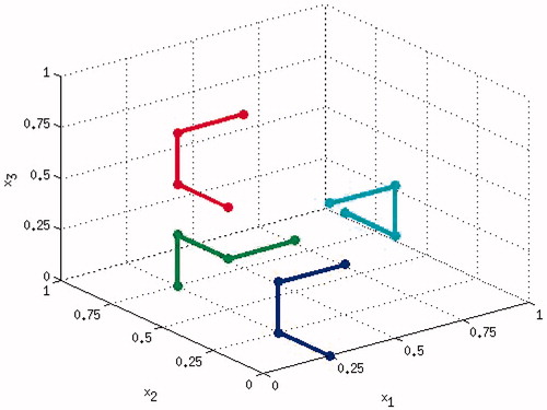
In this way, a local computation of the elementary effects is performed in multiple locations throughout the parameter space. These can be viewed as a set of parameter trajectories through the region of interest in order to obtain a global view of the response of the function y(x). An example of a computational experiment with 4 random starting locations with 3 parameters is shown in Figure 1. The local main effects for each parameter are then averaged and their standard deviation computed. The mean and standard deviation are then the sensitivity measures used in the Morris Method. The mean indicates the magnitude of the main effects for each parameter and the standard deviation takes into account the effect of varying other parameters and provides a qualitative measure of the non-linear interaction.

Figure 1. A graphical representation of the sampling strategy in the Morris method for three parameters. Four random starting points are selected and then trajectories are formed from these so that three main effects can be computed for each starting location.

Mathematical model of RFA

The mathematical model used in this study is based on that developed by Trujillo et al. [4,5]. The main difference is the inclusion of a different cell death model and the selection of a specific set of functions to describe the temperature dependence of various tissue properties. This model has been chosen for this sensitivity analysis because it is representative of those commonly used in the literature: it captures a wide range of the physical processes that are occurring during RFA, ensuring that it is as general a model as currently available. The axisymmetric geometry used here is nearly identical, the only difference being that the applicator modelled here has a solid metal active tip, as shown in Figure 2.

Figure 2. Axisymmetric geometry adapted from Trujillo et al. [4,5].

The model consists of three main parts: a bioheat transfer model, an applicator (heat source) model and a cell death model. The full model is a coupled non-linear system of partial differential equations that can be solved by a variety of numerical methods. The constituent equations are presented here along with a brief description of the implementation. The code to reproduce these results along with a more in-depth explanation is available as open source software at: https://github.com/sheldonkhall/MITA-model. The numerical methods used to obtain accurate solutions are not considered further here and it is assumed that numerical errors are far smaller than the modelling and experimental errors.

Bioheat transfer

In order to compute the evolution of the system over time, including the dominant physical processes, the apparent heat capacity form of the Pennes equation is solved [6–8]. This is given by Equation 2(2) $\rho c_{\mathrm{app}}\left(T\right)\frac{\partial T}{\partial t}=\nabla ·k\left(T\right)\nabla T-\omega \left(T\right)c_b{\rho }_b[T-T_0]+Q\left(T\right),$(2) : (2) $\rho c_{\mathrm{app}}\left(T\right)\frac{\partial T}{\partial t}=\nabla ·k\left(T\right)\nabla T-\omega \left(T\right)c_b{\rho }_b[T-T_0]+Q\left(T\right),$(2) where t is time in s, T is the temperature in K, k is the thermal conductivity, ω is the blood perfusion in 1/s, c_b is the specific heat capacity of blood in J/kg/K, ρ_b is the density of blood, T₀ is the baseline physiological temperature taken to be 310 K and Q is the heat source generated by the probe in W/m³. The apparent specific heat term, ρc_app, is given by Equation 3(3) $\rho c_{app}=\{\begin{array}{r}\hfill \rho c,T\le T_l\\ \hfill \frac{\rho c+{\rho }_{vap}{c}_{vap}}{2}+{\rho }_{w}LC\frac{1}{T_u-T_l}+,T_l<T\le T_u\\ \hfill {\rho }_{vap}{c}_{vap},T_u<T\end{array},$(3) (3) $\rho c_{app}=\{\begin{array}{r}\hfill \rho c,T\le T_l\\ \hfill \frac{\rho c+{\rho }_{vap}{c}_{vap}}{2}+{\rho }_{w}LC\frac{1}{T_u-T_l}+,T_l<T\le T_u\\ \hfill {\rho }_{vap}{c}_{vap},T_u<T\end{array},$(3) where ρ and ρ_vap are the density (kg/m³) of normal and vaporised tissue respectively, c and c_vap are the specific heat (J/kg/K) of normal and vaporised tissue respectively, ρ_w is the density of water, L is the latent heat of vaporisation (J/kg) and C is the tissue water fraction. Water inside the tissue is assumed to vaporise over a range of temperature in tissue defined by T ∈ [T_l,T_u], where T_l and T_u are the lower and upper temperature respectively, because it is in a mixture and no longer a pure substance.

At the external tissue boundaries a Dirichlet condition is set to ensure that the temperature remains at T₀ the physiological temperature. On the plastic components of the applicator an insulating Neumann boundary is applied to ensure no heat flows into the plastic. The cooling of the probe is modelled by applying a convective heat transfer condition h(T−T₀) to the active tip. In this study a value of h=3366 W/K/m² was used.

Thermal conductivity k

The thermal conductivity is commonly set to a constant value in the literature due to the fact that this is thought to have only a limited impact on the results. For the purpose of the sensitivity analysis here, a more complicated dependence on temperature has been included with an initial linear rise. Further, when considering phase change, the functional form of k must be valid at T > 373 K. In order to do this, a piecewise continuous function is used [5] (4) $k\left(T\right)=\{\begin{array}{ll}{k}_0+\Delta k[T-T_0],\hfill & T\le 373 K\hfill \\ k_0+\Delta k[373-T_0],\hfill & T>373 K\hfill \end{array},$(4) where k₀ is the baseline thermal conductivity, Δk is the change in k per Kelvin and T₀ is the reference temperature at which k₀ has been measured, which in this case is the same as the physiological temperature.

Perfusion ω

Perfusion has been observed to have a large impact on simulations of RFA and its dependence on temperature is complex [9]. Blood perfusion is known to stop within the coagulation zone due to collapse of the vasculature, after an initial rise which is due to the body’s homeostatic mechanisms trying to reduce the local temperature [10]. In this model, the dependence of the perfusion term on temperature is related to the cell death model via the viability G. A simple perfusion term is used in our model because little quantitative information about the variation in the liver is available in the literature. The perfusion is computed using Equation 5(5) $\omega \left(G\right)=\{\begin{array}{cc}{\omega }_0,& G>G_0>\\ 0,& G\le G_0>\end{array},$(5) (5) $\omega \left(G\right)=\{\begin{array}{cc}{\omega }_0,& G>G_0>\\ 0,& G\le G_0>\end{array},$(5) where ω₀ is the baseline blood perfusion and G₀ the viability threshold for the collapse of the vasculature. Once a certain cell viability is reached, it is assumed that complete destruction of the tissue will occur. The lesion size is determined using this threshold and therefore the collapse of the vasculature is assumed to occur in the same zone.

Electric potential solver (RFA)

In order to determine the heat deposited by the probe, a simplified form of Maxwell’s equations is solved. Due to the large difference in the timescales of the electrical and thermal problems, a quasi-static approximation can be made and a solution found in terms of the electric potential V can be determined by Equation 6(6) $\nabla ·\sigma \left(T\right)\nabla V=0,$(6) (6) $\nabla ·\sigma \left(T\right)\nabla V=0,$(6) where σ is the electrical conductivity. This is subject to Dirichlet boundary conditions on the probe surface and on the external surfaces [11]. The probe voltage is set to V_probe=60V and the voltage on the external tissue boundary to V=0, which establishes a potential difference similar to that between the probe and ground pads in a patient. This drives current through the tissue resulting in resistive heating. The generated heat can then be computed using Equation 7(7) $Q=\sigma \left(T\right){\left|\nabla V\right|}^2.$(7) (7) $Q=\sigma \left(T\right){\left|\nabla V\right|}^2.$(7)

Electrical conductivity σ

The electrical conductivity is commonly described by a linear function of temperature [5] as in Equation 8(8) $\sigma \left(T\right)={\sigma }_0+\Delta \sigma [T-T_0],$(8) (8) $\sigma \left(T\right)={\sigma }_0+\Delta \sigma [T-T_0],$(8)

It has been observed that electrical conductivity has a dependence on temperature, although it has not been conclusively determined exactly what functional form this follows. When considering phase change, the functional form of the electrical conductivity σ must be valid at T > 373 K because of the impact of the changing water content of tissue on the conductivity. In order to do this, a piecewise continuous function is used [5] as in Equation 9(9) $\sigma (T)=\{\begin{array}{c}{\sigma }_0+\Delta \sigma \left[T-T_0\right],T\le T_u\\ \begin{array}{c}\frac{\left[{\sigma }_{vap}-\left[{\sigma }_0+\Delta \sigma \left[T_u-T_0\right]\right]\right]\left[T-T_u\right]}{5}+{\sigma }_0\\ +\Delta \sigma \left[T_u-T_0\right],T_u<T\le T_u+5\end{array}\\ {\sigma }_{vap},T_u+5<T\end{array},$(9) : (9) $\sigma (T)=\{\begin{array}{c}{\sigma }_0+\Delta \sigma \left[T-T_0\right],T\le T_u\\ \begin{array}{c}\frac{\left[{\sigma }_{vap}-\left[{\sigma }_0+\Delta \sigma \left[T_u-T_0\right]\right]\right]\left[T-T_u\right]}{5}+{\sigma }_0\\ +\Delta \sigma \left[T_u-T_0\right],T_u<T\le T_u+5\end{array}\\ {\sigma }_{vap},T_u+5<T\end{array},$(9)

where σ₀ is the baseline conductivity, Δσ is the change in the conductivity per degree Kelvin, T₀ is the reference temperature at which σ₀ has been measured and σ_vap is the conductivity of vaporised tissue. This model describes an initial linear rise of the electrical conductivity until the phase change temperature at which there is a drastic drop to an almost zero value as tissue water is converted to gas.

Impedance control system

Commercial RFA systems are controlled by adjusting the applied voltage to ensure either that the deposited power remains constant, that the maximum temperature is never exceeded or that the impedance does not cross a threshold indicating extensive vaporisation [11]. The impedance of the tissue between the probe and the ground pads is an ideal indicator of the presence of vaporisation near the probe surface, and for this reason it is used to control the power deposition during RFA.

In this model an impedance threshold of R=120 Ω is defined, above which the heat source is set to zero for a period of 15 s [4,5] to allow the tissue to cool and any generated gas to dissipate from the near vicinity of the probe. In the approximation being used to compute the electric potential, the resistance can be computed using Equation 10(10) $R\left(t\right)=\frac{V^2(t)}{P_{\mathrm{total}}(t)},$(10) (10) $R\left(t\right)=\frac{V^2(t)}{P_{\mathrm{total}}(t)},$(10) where R(t) is the resistance, V(t) is the applied voltage and P_total(t) the power deposited in the tissue. P_total(t) is computed by integrating the heat source, Q, over the computational domain [12] as in Equation 11(11) $P_{\mathrm{total}}(t)=\int Q(t,r)\mathrm{dV},$(11) . (11) $P_{\mathrm{total}}(t)=\int Q(t,r)\mathrm{dV},$(11) where r is the position vector from the origin.

Cell death model

The cell death model used in this study is that developed by O’Neill et al. [13]. This model is a system of three ordinary differential equations (ODEs) representing the proportion of cells in an alive, dead or vulnerable state. The inclusion of the vulnerable state is a result of the direct observation of cells under thermal insult and results in better agreement with experimentally observed viabilities. The system of equations reduces to two ODEs due to the constraint that A+V+D=1, where the proportions of alive, vulnerable and dead cells are given by A, V and D respectively. The system of ODEs is (12) $\frac{\mathrm{dA}}{\mathrm{dt}}=-k_{f}A+k_b[1-A-D],$(12) (13) $\frac{\mathrm{dD}}{\mathrm{dt}}=k_f[1-A-D],$(13) where (14) $k_f={\overline{k}}_f{e}^{T/T_k}[1-A].$(14)

The model has three parameters: ${\overline{k}}_f$, k_b and T_k which were all obtained via fitting to experimental data from cell culture experiments. The cell viability, G=1−D, is used to determine the lesion size and the cessation of perfusion, and represents the proportion of cells that are not dead, i.e. including alive and vulnerable. This is done by defining a threshold of G₀, below which the perfusion stops and all cells are expected to die.

Model summary

The full system of equations describing RFA in this study is thus: (15) $\begin{array}{cc}\multicolumn{1}{c}{\rho c_{\mathrm{app}}\left(T\right)\frac{\partial T}{\partial t}}& =\nabla ·k\left(T\right)\nabla T-\omega (1-D)c_b{\rho }_b[T-T_0]\hfill \\ \multicolumn{1}{c}{}& \mathrm{\hspace{1em}\hspace{1em}\hspace{1em}}+\sigma \left(T\right){\left|\nabla V\right|}^2,\hfill \end{array}$(15) (16) $\nabla ·\sigma \left(T\right)\nabla V=0,$(16) (17) $\frac{\partial A}{\partial t}=-k_{f}A+k_b[1-A-D],$(17) (18) $\frac{\partial D}{\partial t}=k_f[1-A-D].$(18)

The model equations used here are non-linear and require a relatively complicated iterative scheme to ensure that the solution converges to the correct answer in an efficient manner. A bioheat solver was created using FEniCS [14], an open source framework for solving differential equations using the finite element method. The specific implementation has been released as open source software and will only be described briefly here.

The bioheat equation is solved using an adaptive method in time to ensure that the time step is small enough to capture the energy required to produce phase change [15]. The advantage is that the sizes of the time steps required are so small that no iterations are required to resolve the non-linearities in the model. The previous iteration temperature can be used as input for the current iteration, essentially a single Picard iteration at each time step. For each computation of the temperature, the source term must be recomputed via a calculation of the electrical potential V.

The cell death model is solved using a generic adaptive ODE solver that requires different time step sizes from those used in the bioheat equation to achieve the target accuracy. At each time step the values for A and D from the previous time step are used in the bioheat equation. The viability for the current time step is computed by assuming that the temperature is constant over the time interval and the system of equations is solved using the ODE solver for this period using initial conditions from the previous time step.

Physiological parameters

Now that the model being used in the sensitivity analysis has been presented, an in-depth analysis of the available parameter values and their uncertainties is required. It has been observed that organs differ greatly with respect to blood perfusion, density and procedure outcome according to modality. RFA is commonly performed on the liver, and for this reason there exist multiple measurements of the physiological parameters used in the mathematical models. Therefore, we have restricted our analysis to models of RFA on liver to ensure that we have as much parameter information as possible in order to perform the analysis, and that the results are meaningful by restricting the validity of the parameters to a single organ. We have found no information about the probability distribution of the parameters and therefore it is assumed here that the probability density function is uniform over the range given by the uncertainty.

There are 19 parameters in total under consideration, with all other quantities considered as constants. These 19 parameters are: c, c_vap, c_b, ρ, ρ_vap, ρ_b, T_l, T_u, σ₀, Δσ, σ_vap, k₀, Δk, ω_b, ${\overline{k}}_f$, k_b, T_k, C and G₀. The available literature has been reviewed to extract as much primary information as possible about each parameter. Where the primary resource could not be obtained, the article used and the primary source (if clear) are cited together. The purpose of this section is not to assess the different options for modelling the dependencies of the parameters, since this decision has been made already. Rather, the aim is to derive a range of values representing the uncertainty in a specific parameter, for the chosen model. The range of values is selected such that hopefully it contains contributions from all of the major sources of uncertainty: experimental error, variation amongst the population and errors from using similar but not identical tissues.

The parameter values in the literature are stated in a variety of units as a result of being measured for different applications or reflecting a more universal acceptance of SI units. In some cases the conversion of quoted values to SI units is trivial and will not be elaborated on. In others, most notably blood perfusion, this is not the case and the conversion will be given explicitly. Finally, it should be noted that there exists an online database of physiological properties with standard deviation and maximum and minimum values [16]. Existing values for the parameters under consideration will be contrasted against the chosen ranges.

Specific heat capacity (J/kg/K)

The specific heat capacity of the liver is available for multiple species in a variety of conditions. The raw data are presented in Table 1 and are too sparse from which to draw any definitive conclusions. For normal tissue at physiological temperatures, the mean value is c≈3700 J/kg/K and it is not clear whether the variations seen are due to measurement uncertainty, variations between species, or variations within a species. There does, however, appear to be a trend of increasing specific heat capacity with temperature, which can be seen in the porcine data.

Table 1. Values of the specific heat capacity of liver ± standard deviation with references.

c	± SD	Species	T	Sample	Tissue	Reference
3411		Bovine	298	In vitro	Normal	[17]
3690	70	Bovine	310	Ex vivo	Normal	[18]
3650	90	Bovine	310	Ex vivo	F-Co	[18]
4187		Bovine	357	In vitro	Normal	[17]
3598		Human	273–298	Ex vivo	Normal	[19]
3758	66	Human	310	Ex vivo	Tumour	[18]
3617	78	Human	310	Ex vivo	Normal	[18]
3730	150	Porcine	310	Ex vivo	Normal	[18]
3720	180	Porcine	310	Ex vivo	F-Co	[18]
3660	100	Porcine	310	Ex vivo	F-T	[18]
3480	100	Porcine	310	Ex vivo	F-T-Co	[18]
3628		Porcine	293–343	Ex vivo	Normal	[20,21]
3858		Porcine	353–373	Ex vivo	Normal	[20,21]
3986		Porcine	383–393	Ex vivo	Normal	[20,21]
3690						[22]
3629						[23,24]
3600						[25]

Blank spaces denote incomplete information in the source. SD, standard deviation; F, freeze; T, thaw; Co, coagulated).

The temperature dependence of the specific heat capacity is often omitted in mathematical models of RFA. Therefore, to determine whether variations of the size observed in Table 1 have a significant effect on the model predictions, the range of the specific heat capacity will be set to c ∈ [3600, 4000] J/kg/K. Another advantage of choosing this range is that it also includes the specific heat capacity of coagulated tissue. It should be noted that tumour tissue is highly heterogeneous and there is not enough information available to determine whether the range of values in tumour tissue are different to that defined here [16].

Density (kg/m³)

Primary sources for measurements of liver density in the literature are again sparse. The similarity observed between the values also indicates that some may be from the same source, but this could not be determined definitively and thus all are provided in Table 2. The variation in the values is relatively small and, ignoring the identical values, the mean is ρ=1050 kg/m³. Using the maximum and minimum values, the range of density is set to ρ ∈ [1020, 1080] kg/m³.

Table 2. Values for the density of liver with references.

ρ	Species	T	Sample	Tissue	Reference
1050	Human		Ex vivo	Normal	[19]
1020	Porcine	293–343	Ex vivo	Normal	[20,21]
1050					[23,24]
1080					[22]
1060					[25,26]
1050					[25,27,28]

Blank spaces denote incomplete information in the source.

Thermal conductivity (W/m/K)

The model of thermal conductivity given in Equation 4(4) $k\left(T\right)=\{\begin{array}{ll}{k}_0+\Delta k[T-T_0],\hfill & T\le 373 K\hfill \\ k_0+\Delta k[373-T_0],\hfill & T>373 K\hfill \end{array},$(4) contains three parameters: the baseline thermal conductivity, the rate of change of the thermal conductivity and the temperature at which vaporisation occurs. The vaporisation temperature is chosen to be the boiling point of water T_u=373 K here and the literature values of the remaining parameters are given in Tables 3 and 4. The model utilised in this study ignores the impact of perfusion on the thermal conductivity.

Table 3. Baseline values of thermal conductivity k₀ in W/m/K.

k0	Species	T	Sample	Tissue	Reference
0.565	Human	278	Ex vivo	Normal	[19]
0.512	Human	276–318	Ex vivo	2 days saline	[29]
0.465	Porcine	293–343	Ex vivo	Normal	[20,21]
0.867	Porcine	353–373	Ex vivo	Normal	[20,21]
1.46	Porcine	383–393	Ex vivo	Normal	[20,21]
0.46–0.49					[22]
0.565					[23,24]

Blank spaces denote incomplete information in the source.

Table 4. Rate of change of thermal conductivity Δ k in W/m/K².

Δ k	Species	T	Sample	Tissue	Ref
0.001161	Human	276–318	Ex vivo	Normal	[29]
0.0033	Bovine	298–353	Ex vivo	Normal	[30]

The only two confirmed sources of baseline thermal conductivity data for human liver result in a mean value of k=0.539 W/m/K. If the last two values in Table 3 are also considered, as they have been used in simulations, then the range of thermal conductivity would be k ∈ [0.46, 0.57]. This is a large range, but is assumed here in order to reflect the range of expected values in the absence of any further information.

The rate of change of thermal conductivity in humans for a linear model is only available from one source. Another value is available for bovine liver, which is histologically similar; however, this does not inform us greatly about the variation amongst humans. It has been noted in the literature that mathematical models of RFA are not very sensitive to temperature-dependent variations in k [5]. For this reason, the range of values for the rate of change of the thermal conductivity is chosen to be Δk ∈ [0, 0.0033] W/m/K². The sensitivity of the model to this parameter will hopefully provide information about the validity of using histologically similar material or excluding the temperature dependence of thermal conductivity completely by setting Δk ≡ 0.

Electrical conductivity (S/m)

Data are available over a wide range of frequencies for the electrical conductivity in human tissue; however, it is noted that the variation between species is likely to be less than the variations within a single species [25,31]. This means that the results of studies into histologically similar tissue from other species can provide valuable information. The results of the wide-band experiments are usually fitted to a Cole–Cole relationship [32] to describe the variation with frequency, and the data points often do not coincide exactly with the frequencies used in RFA. Therefore, to extract some values, interpolation has been used. This seems appropriate given the errors and number of data points. The data are summarised in Table 5.

Table 5. Electrical conductivity σ in S/m of liver tissue.

σ	± SD	Species	T	f (MHz)	Sample	Tissue	Reference
0.141		Human	310	0.1	Ex vivo	Normal	[25]
0.227		Human	310	1.0	Ex vivo	Normal	[25]
0.19–0.45		Human	296–298	0.1	Ex vivo	Normal	[32]
0.24–0.28		Human	296–298	1.0	Ex vivo	Normal	[32]
0.277	15–25%	Human		0.5	Ex vivo	Normal	[33]
0.26	0.06	Human		0.46	Ex vivo	Normal	[34]
0.5	0.2	Human		0.46	Ex vivo	MCT	[34]
0.333				0.5			[35,36]
0.148				0.5			[33,37]

Blank spaces denote incomplete information in the source. SD, standard deviation; MCT, metastatic colorectal tumour.

The frequencies at which the electrical conductivity has been measured are in the range 0.1–1.0 MHz, and the values of electrical conductivity for normal human liver lie in the range σ ∈ [0.14, 0.28] S/m excluding the value of 0.333 S/m from Haemmerich [9], because an experimental source could not be determined and as this appears to be an outlier. This range of values appears to represent the variation seen in the experimental data and will thus be used in the sensitivity analysis.

There are also data available for the rate of change of the electrical conductivity in histologically similar tissues and these are given in Table 6. Data on the rate of change of electrical conductivity are much harder to find and values derived from multiple species and different organs are used due to a lack of better sources. The choice of the parameter range in this case is fairly arbitrary but is chosen to be $\Delta \sigma \in [1,2]$%/K to capture the full range of observed values at ≈0.5 MHz.

Table 6. Rate of change of the electrical conductivity in %/K.

Δ σ	± SD	Species	Organ	T	f (MHz)	Reference
1.62	0.04	Porcine	Kidney	321–351	0.46	[38]
0.6–1.3		Mixed	Liver		0.1–1	[25]
2		Mixed				[25,39]
2		Mixed				[40,41]

Blank spaces denote incomplete information in the source. SD, standard deviation.

Once the tissue has vaporised, the electrical conductivity is hypothesised to drop dramatically due to the change in water content. This is analogous to the changes observed during measurement of the electrical properties during MWA. The value of the electrical conductivity in vaporised tissue has been assumed to be two to four orders of magnitude smaller [5] and for this study, we will assume a range of values ${\sigma }_{\mathrm{vap}}\in [0.0001,0.01]$ × σ₀ to test whether there is any significant difference in the solution as a result.

Blood perfusion (s⁻¹)

When assessing blood perfusion data it becomes apparent very quickly that the largest variety of definitions exist for this parameter. There is no ambiguity in converting these to a definition useful for the Pennes equation; however, some conversions require the use of other physiological parameters, namely ρ, ρb and c_b. This will introduce further uncertainty into the perfusion values. Due to the large variability in perfusion, however, it will be assumed that the uncertainty in ρ, ρb and c_b is dominated by that found in the measurement of perfusion in whatever form. To ensure consistency, the following values are used for conversions $\rho \equiv {\rho }_b=1050$ kg/m³ and $c_b=3600$ J/kg/K, aside from the standard conversion to SI units. The quoted values and their conversion to SI units of s⁻¹ corresponding to the volumetric flow of blood per unit tissue volume are given in Table 7.

Table 7. Blood perfusion (ω) values for the liver converted to consistent units of s^-1.

Value	± SD	Unit	Conversion	ω (s^−1)	± SD	Species	Tissue	Reference
108	34	mL/100 mL/min	10^−2/60	0.018	0.006	Human	Normal	[42]
98	36	mL/100 mL/min	10^−2/60	0.016	0.006	Human	d	[42]
70	22	mL/100 mL/min	10^−2/60	0.012	0.004	Human	ca	[42]
69	30	mL/100 mL/min	10^−2/60	0.012	0.005	Human	cb	[42]
56	13	mL/100 mL/min	10^−2/60	0.009	0.002	Human	cc	[42]
1000/1100		mL/kg/min	1/10^6/60 × ρ	0.018/0.019		Human m/f	Normal	[43]
100	20	mL/100 mL/min	10 × ρ/60/10^6	0.018	0.004			[22]
9.19		kg/m^3/s	1/ρb	0.009				[23,24]

Blank spaces denote incomplete information in the source. SD, standard deviation; m, male; f, female; d, diseased non-cirrhotic; ca, child a; cb, child b; cc, child c.

The data appear to cover a large range of values, including baseline values and those of diseased livers. The average of all the normal values of liver perfusion is $\omega \approx 0.016$ s⁻¹. It is assumed this represents the variation seen within the population and the range of perfusion values used in this study is chosen to be $\omega \in [0.009,0.018]$ s⁻¹. The diseased livers, predominantly cirrhotic, appear to have a lower perfusion and it is beneficial that these are included in the range as it is likely that they have a significant impact on the predictions.

Water content of tissue

The water content of liver tissue is presented in Table 8 along with the sources. The values for the water content of tissue are given either by mass or volume fraction, and conversion between the two values is not necessary due to the size of the uncertainty. The last two values in the table do not have a clear experimental source and therefore are neglected in this study. Taking the remaining values of the water content, it is assumed that $C\in [0.71,0.76]$ in this study.

Table 8. Water content C of liver tissue.

C	± SD	Units	Species	Reference
0.73		MF	Bovine	[44]
0.71	0.045	MF	Bovine	[45]
0.77		MF	Human	[19]
0.72–0.76		VF		[25,26]
0.68		VF		[46]
0.78		MF		[47]

Blank spaces denote incomplete information in the source. MF, mass fraction; VF, volume fraction.

Phase change temperature range (K)

The phase change temperature range has not necessarily been measured, but phase change occurs over a range of temperatures in non-pure substances such as tissue. This is utilised in models of cryosurgery to simplify the numerical solution procedure, but less research has been conducted for vaporisation of the water content of tissue. The temperature over which phase change is assumed to occur is normally set to be 1 K [48]; given that not much is known about this process, a range of $\Delta T\in [1,\mathrm{\hspace{1em}\hspace{1em}}10]$ K will be chosen for this study. The results will hopefully shine light on the adequacy of the current values used.

Vaporised tissue thermal properties (J/m³/K)

The thermal properties of vaporised tissue are not readily available; however, two values have been found in the literature. One is quoted in terms of ${\rho }_{\mathrm{vap}}{c}_{\mathrm{vap}}$ and therefore the other has been converted to this form for comparison, as it can be used in this form in the sensitivity analysis. The two values are ${\rho }_{\mathrm{vap}}{c}_{\mathrm{vap}}=800$ kJ/m³/K [46] and ${\rho }_{\mathrm{vap}}{c}_{\mathrm{vap}}=440$ kJ/m³/K [48,9,49]. These are not necessarily for the same tissue and the variability reflects how little is known about this parameter. With no other information available, the range has been set to ${\rho }_{\mathrm{vap}}{c}_{\mathrm{vap}}\in [400,800]$ kJ/m³/K. This is significantly less than the value in normal tissue, and the impact on the results is as yet unknown.

Cell death model parameters

The cell death model used here is taken from O’Neill et al. [13] and this reference provides the only available parameters for this model. The available parameters are for two pure cell cultures, lung fibroblast MRC-5 and hepatocellular carcinoma HepG2, and mixtures of these cell lines. It is proposed here that the range of parameter values between the two pure cell cultures be used to represent the magnitude of the variation in the population and to capture any difference between parameter values in culture and tissue in vivo. The ranges are: ${\overline{k}}_f\in [0.80,\mathrm{\hspace{1em}\hspace{1em}}9.07]$ × 10⁻³ s⁻¹; $k_b\in [0.25,\hspace{1em}19.2]$ × 10⁻³ s⁻¹; and $T_k\in [24.6,\hspace{1em}63.5]$ °C. However, since the parameter values appear to be highly correlated and randomly selecting values in these ranges will result in spurious results, the three parameters will be varied using a single parameter $\xi \in [0,\mathrm{\hspace{1em}\hspace{1em}}1]$ which represents the composition of the cell culture, ξ = 0 representing a pure HepG2 culture. A linear interpolation is used on the parameter values presented in Table 4 of the O’Neill et al. paper [13] to return intermediate values. This is sufficient for this analysis as it will allow the parameters to vary over the whole range without producing spurious results.

A further parameter is also involved with determining the ablation zone size. This is the threshold that determines subsequent cell death after the procedure has finished. It has been observed that the ablation zone seen immediately post-intervention will grow slightly in the days following treatment. Based on this observation and cell culture experiments, it was determined that all regions with $G_0\le 80$% cell viability should represent the lesion volume. Due to the sparsity of the data and the differences between the behaviour of cells in culture and tissue, it is very difficult to ascertain a range of values that is representative. It is expected that the results will be very sensitive to this parameter, and therefore picking an artificially large range will bias the results. For this reason the range of $G_0\in [70,\mathrm{\hspace{1em}\hspace{1em}}90]$% is chosen as it represents the range over which there were no data available in O’Neill et al. [13] to determine an exact value for the threshold for the cell culture experiments. This threshold is also used to determine the region in which there is no perfusion as it is assumed that the ablation zone marks the lower bound of the unperfused region during the procedure.

Summary values

The parameter values used in the sensitivity study are summarised in Table 9. The values determined in this study are contrasted against those given in the IT’IS database [16]. Good agreement is seen between the values and this is interpreted as implying a sensible choice for the ranges. There are fewer parameters in the summary table than have been identified in the model and this is due to some simplifications that allow the number of parameters to be reduced, which will have a positive impact on computing times.

Table 9. Summary of parameter value ranges used in the sensitivity study given as a range. These are contrasted against the IT’IS database [16].

Parameter	Range	IT’IS mean ± SD	IT’IS range	IT’IS no. of studies
c (J/kg/K)	3600–4000	3540 ± 119	3332–3617	5
ρ (kg/m^3)	1020–1080	1079 ± 53	1050–1158	4
k (W/m/K)	0.46–0.57	0.52 ± 0.03	0.48–0.57	9
Δ k (W/m/K^2)	0–0.0033
σ (S/m)	0.14–0.28	0.144
Δ σ (%/K)	1–2
ω (s^-1)	0.009–0.018	0.015 ± 0.003	0.007–0.022	50
C	0.71–0.76
Δ T (K)	1–10
ρvap cvap (J/m^3/K)	440,000–800,000
ξ	0–1
σvap/σ	0.01–0.0001
G0 (%)	70–90

Blank spaces denote information unavailable in the IT’IS database.

The first simplification is related to the relative size of the uncertainties in given parameters. When considering the term in the bioheat equation that accounts for the heat sink produced by perfusion, $\omega {\rho }_b{c}_b[T-T_0]$, the uncertainty in blood perfusion ω dominates over that of the density and specific heat capacity of blood. This allows variations in the perfusion to be included in the analysis, and those of the blood thermal properties to be omitted. This is done by defining a new parameter ${\omega }_b\in [{\omega }_{\mathrm{lower}}{\rho }_b{c}_b,{\omega }_{\mathrm{upper}}{\rho }_b{c}_b]$ J/m³/K/s.

Instead of having two independent parameters for the lower and upper temperatures at which phase change occurs, a single parameter $\Delta T\equiv T_u-T_l$ is defined and the upper temperature range is set to the boiling point of water $T_u\equiv 373$ K. The effective specific heat ρ c_app also contains the term ${\rho }_w\mathrm{CL}/\Delta T$, which will be dominated by the errors in water content, C, and the temperature range, Δ T.

The parameters ρ and c always appear as a product and for this reason all instances will be treated as a single parameter that is varied over the range of uncertainty of both parameters. The final set of parameters used in the sensitivity analysis and their values are thus given in Table 10.

Table 10. Final set of parameters included in the sensitivity analysis.

Parameter	Units	Lower	Upper
ρc	J/m^3/K	3.7 × 10^6	4.3 × 10^6
ρvap cvap	J/m^3/K	0.44 × 10^6	0.80 × 10^6
k0	W/m/K	0.46	0.57
Δ k	W/m/K^2	0	0.0033
σ0	S/m	0.14	0.28
Δ σ	%/K	1	2
ω b	J/m^3/K/s	34,020	68,040
C		0.71	0.76
Δ T	K	1	10
ξ		0	1
σvap/σ		0.01	0.0001
G0	%	70	90

Results

The Morris method was used with six random orientations and 12 parameters for a total of 78 numerical experiments performed using our model. The results are usually displayed on a 2D scatter plot with the mean values of the main effects along the x-axis and the standard deviations of the main effects along the y-axis. In addition to this, the line y = ± x is added to demonstrate whether the magnitude of the main effect is larger than the standard deviation, i.e. it is likely that the main effect is non-zero. It has also been suggested that a third sensitivity measure, the mean of the absolute value of the main effects, is used to identify non-monotonic responses [50]. For our results it was found that this measure did not provide further information and the results have been omitted.

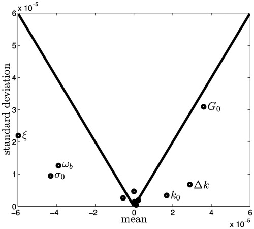
In this study one of the critical predictions is the size of the ablation zone, and the sensitivity of the size of the ablation zone to the parameters at the end of the simulation is shown in Figure 3. Four parameters: (1) perfusion ω b, (2) cell composition fraction ξ, (3) viability threshold G₀ and (4) baseline electrical conductivity σ₀ are found to be clearly distinct from the cluster near zero of the remaining parameters. These four are the most important parameters in the model, and because they lie below the line y = ± x, the main effect is likely to be non-zero while the non-linear and interaction effects are likely to be less dominant. Conversely, the parameters near zero are both above and below the line and are relatively small, and their impact on the ablation zone size is unlikely to be significant. The thermal conductivity and rate of change of thermal conductivity, k₀ and Δ k respectively, also appear distinct from the cluster at zero, but less important than the other parameters.

Figure 3. Results of the Morris method when considering the ablation zone size at the end of the procedure. The means of the main effects are plotted along the x axis and the standard deviations along the y axis. The solid line is plotted for y = ± x and for points below the line the mean is larger than the standard deviation and therefore the expected value of the mean is non-zero.

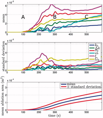
The importance of the parameters can additionally change over time, and for this reason the means and standard deviations are plotted against time in Figure 4. Three regions can be observed in the transient sensitivities: (1) an initial phase t < 200 s, where no tissue has crossed the viability threshold; (2) a transient phase 200 < t < 400 s, where the sensitivities transition from short- to long-term values, briefly having standard deviations that are similar in size to the mean; and (3) steady-state t < 400 s, where the dominant parameters on the final ablation zone size are identified and those involved only in the transient behaviour lose significance. A plot of the mean ablation zone size ± standard deviation has also been plotted on the same time scale as the sensitivity measures. This gives an idea of how much of an effect the parameter changes have on the model predictions. The sensitivity coefficients can also be integrated over time in order to determine some averaged value for the whole simulation, but in this case the results were found to differ negligibly from those at the end of the simulation.

Figure 4. Sensitivity measures plotted versus time and contrasted against the mean ablation zone area. The long-term behaviour is of interest here and it can be seen that σ₀, ω_b, ξ and G₀ have the greatest impact on the ablation zone area due to their relatively large mean. The standard deviations are also larger for some of these parameters, indicating parameter interactions or non-linear responses. A, B, and C denote initial, steady-state, and transient periods respectively.

The Morris method results for the area defined by T ≥ 50 °C are also of interest because isotherms have been used previously to define the lesion size. The sensitivity data for this isotherm are very noisy and challenging to interpret, changing drastically between times when the heat source is on and off. Further, as the time extends beyond t = 100 s, the times at which the source is switched on and off become increasingly out of phase in the different experiments. This difference in the on/off times of the various numerical experiments obscures the information contained in the sensitivities. However, some information can be obtained by observing the sensitivities in the initial phase. The mean and standard deviation of the isotherm area are shown alongside the parameter sensitivities for t ≤ 100 s in Figure 5.

Figure 5. Sensitivity measures for the 50 °C isotherm versus time contrasted against the mean area. The changes in the area of the isotherm are complex but are separated into regions of (A) active heating and (B) cooling. During the initial heating phase σ₀ and dominates. During cooling the thermal parameters perfusion ω_b, baseline thermal conductivity k₀ and rate of change of thermal conductivity Δk are the most important.

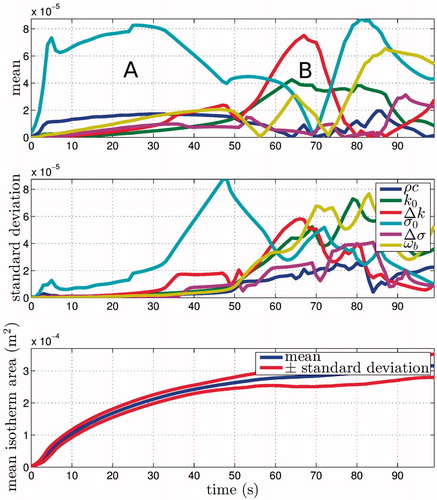
During the initial period of active heating (A in Figure 5) the baseline electrical conductivity σ₀ appears to dominate. Eventually the impedance spikes in the simulation and the heat source is switched off (B in Figure 5). During this cooling period a different set of parameters becomes important. As expected, these are related to the thermal properties of the tissue and are: (1) baseline thermal conductivity k₀, (2) rate of change of thermal conductivity Δk and (3) blood perfusion ω b.

Discussion

Currently, sensitivity analyses of models of RFA are restricted to varying very few parameters and observing the differences in a prediction of interest. In contrast, in this work the Morris method has been applied to analyse all of the model parameters at once in an efficient manner. This has the dual objective of bringing together the many disparate studies involving varying only a few parameters by reproducing their findings using a single methodology, and presenting novel results made possible by an analysis of this type.

The Morris method is predominantly used for parameter screening; however, due to the high computational expense of obtaining solutions to our model, it has been used for a full sensitivity analysis. The main weakness in the Morris method is the qualitative nature of the results, which require interpretation in order to make decisions. However, it has been widely and successfully used. When considering the ablation zone area, analogous to the ablation zone volume in 3D, it is clear that four parameters dominate. These are 1) cell death composition ξ, (2) cell death threshold G₀, (3) blood perfusion ω b, and (4) baseline electrical conductivity σ₀. These clearly have larger main effects than the other parameters and most have relatively small standard deviations indicating minimal parameter interactions and non-linear responses. The cell death threshold G₀ does have a standard deviation similar in magnitude to its mean, which could be a result of this value controlling the cessation of perfusion during the simulation. When using this model to compare to experimental data, all of the parameters apart from those mentioned above should be set to a fixed value in the specified ranges. The resulting error between experiments and the model predictions can then be attributed to the cell death model, electrical conductivity and perfusion parameters.

The sensitivity of the model to its parameter values changes over time, but given that the quantity of interest is likely to be the final ablation zone size and shape, it is not necessary to consider the transient behaviour in great detail. In order to improve the accuracy of predictions, attention should be focused on obtaining more data about the blood perfusion, electrical conductivity and cell death dynamics. The identification of the large impact that the cell death parameters have on the lesion size prediction has not been made before, especially in the context of the uncertainty in all of the parameters. It may be that the uncertainty has to be accepted in these aspects of the modelling and uncertainty quantification will then become important in order to better understand the impact on the predictions. The variation in the cell death parameters used in this study is driven by cell type and this should be considered in more detail in future studies.

Schutt & Haemmerich investigated the impact of variations in the level of perfusion and the type of perfusion model used in models of RFA using a more complex geometry [51]. Our representative example was expected to draw similar conclusions. The issue of parameter sensitivity and model selection are combined, and therefore we only consider their results from varying the amount of perfusion. The baseline perfusion was varied ω_b ∈ [0.007, 0.024] s⁻¹ to include cirrhotic livers and the standard deviation of their data. This is larger than the variation employed in this study but does not appear to be a limitation. The conclusion of the study was that varying the perfusion can produce increases of up to ≈ 175% in the ablation zone size. This size increase was not seen in our study, perhaps due to the dissimilarity of the model and perfusion ranges. It is observed, however, that perfusion is one of the important parameters, thus confirming the results of the two studies.

If the area of the 50 °C isotherm is analysed with respect to the parameter values, much more complex behaviour is observed. Our results show that during the active heating phase, the most important parameter is the baseline electrical conductivity σ₀. During the cooling period, when there is no current flowing, the blood perfusion ω b, baseline thermal conductivity k₀ and rate of change of thermal conductivity Δk are important. The complete absence of the vaporised conductivity σ_vap parameter in all of the results clearly demonstrates that any value in the range can be selected without significant error. This has an impact on the numerical solution method, with less steep gradients resulting in shorter solution times.

Trujillo & Berjano investigated the mathematical functions used to describe thermal and electrical conductivities in models of RFA [5]. This analysis was also related to model selection, which is a different area of study from what is presented here. The authors do, however, test what impact varying the parameters of an identical linear model have on the solution. They use the time at which the control system first switched off the heat source, ≈120 s, to analyse the models, the claim being that the majority of the lesion is formed in this time. Our model does not agree with this, a predicted lesion not even appearing until ≈ 200 s, behaviour that can be attributed to the different cell death models. Their main observations are that at short times, the functions of σ and k affect the thermal behaviour, heat source on/off and temperature vs time curves, but not the final lesion size, and that the difference of a two to four orders of magnitude drop in electrical conductivity of vaporised tissue σ_vap has little impact on simulations. This agrees with our results above, although in our study the transient sensitivities of k and σ show more complex behaviour.

Chang investigated how temperature and electric field vary in response to changes in perfusion and temperature dependence of the electrical conductivity [37]. The author admits that a limitation of this study is the lack of a coupled cell death model. It is observed that the temperature dependence of both the electrical conductivity and perfusion have an impact on the temperature seen during RFA. Our results do not necessarily disagree; however, the analysis here would contest that accurate modelling of the temperature dependence of electrical conductivity is secondary. If the prediction of the ablation zone is considered of primary importance, then the perfusion and cell death parameters require significant attention.

Our results show that the rate of change of thermal conductivity with respect to temperature, Δ k, has a relatively small impact on the results. The range of this parameter was set to Δ k ∈ [0, 0.0033] W/m/K², indicating that using a value of Δ k = 0 should be just as accurate as Δ k = 0.0033. This effectively allows us to simplify the model by removing the temperature dependence of the thermal conductivity. This agrees with previous research [5], further demonstrating the utility of the sensitivity analysis.

The sensitivity study presented here is only the initial step in a much more comprehensive analysis of the model [1]. For example, the uncertainty in the prediction of ablation zone size can be computed explicitly for problems in which only the most important parameters are included. This would provide much more certainty about the validity of predictions and provide useful information for the validation of any predictive tool. There is no reason why the Morris method cannot be applied to any model of thermal ablation (cryoablation, radiofrequency, microwave, etc.) to identify important parameters and to allow the model to be simplified by setting the insensitive parameters to constant values.

The inclusion of the cell death model in the analysis demonstrates the need to improve the predictions of models of this type, alongside perfusion and electrical conductivity, to increase the accuracy of the ablation zone prediction. The insensitivity of the ablation zone size to many parameters also indicates that a much simpler model is probably more appropriate in modelling RFA; however, care must be taken when doing this. For example, the ablation zone area may not be sensitive to parameters related to modelling the phase change, yet the exclusion of this feature entirely may produce very different results because latent heat is not accounted for.

Conclusion

The size of the predicted radiofrequency ablation zone is dependent on four main parameters: blood perfusion ω b, cell death model parameters ξ, the viability threshold chosen to represent the ablation zone G₀, and the baseline electrical conductivity σ₀. Therefore, to reduce the uncertainty in the predictions of this model, knowledge about these parameters must be increased. If this is not possible, then the uncertainty on the prediction should be quantified for these parameters. All of the other model parameters can be set to any value in the ranges quoted in this paper without any significant impact on predictions of the ablation zone.

If an isotherm is used to compute the sensitivity measures, then at short times, only the electrical conductivity σ₀, thermal conductivity k₀, rate of change of thermal conductivity Δ k and blood perfusion ω b are important. The first is only important during the time that the heat source is active, while the others are important during the cooling phase. The thermal parameters appear to have large standard deviations, which could be a result of interactions with other parameters or non−linearities in the response. This result shows that if accurate temperature predictions are required, for example to validate the model, then a different set of parameters must be considered.

Declaration of interest

This research has been funded by the European Commission under Grant Agreement No. 600641, FP7 Project Go-Smart. The authors alone are responsible for the content and writing of the paper.

References

- Hall SK, Ooi EH, Payne SJ. A Mathematical Framework for Minimally Invasive Tumor Ablation Therapies. Crit Rev Biomed Eng [Internet]. Begel House Inc.; 2014 [cited 2014 Nov 13];42(5):383--417. Available from: http://www.dl.begellhouse.com/journals/4b27cbfc562e21b8,forthcoming,11825.html
- Saltelli A, Chan K, Scott E. Sensitivity Analysis. Chichester: Wiley, 2000
- Morris MD. Factorial sampling plans for preliminary computational experiments. Technometrics 1991;33:161–74
- Trujillo M, Alba J, Berjano E. Relationship between roll-off occurrence and spatial distribution of dehydrated tissue during RF ablation with cooled electrodes. Int J Hyperthermia 2012;28:62–8
- Trujillo M, Berjano E. Review of the mathematical functions used to model the temperature dependence of electrical and thermal conductivities of biological tissue in radiofrequency ablation. Int J Hyperthermia 2013;29:590–7
- Hu H, Argyropoulos SA. Mathematical modelling of solidification and melting: A review. Model Simul Mater Sci Eng 1996;4:371–96
- Voller VR, Swaminathan CR, Thomas BG. Fixed grid techniques for phase change problems: A review. Int J Numer Methods Eng 1990;30:875–98
- Bonacina C, Comini G. On the solution of the nonlinear heat conduction equations by numerical methods. Int J Heat Mass Transf 1973;16:581–9
- He X, McGee S, Coad JE, Schmidlin F, Iaizzo PA, Swanlund DJ, et al. Investigation of the thermal and tissue injury behaviour in microwave thermal therapy using a porcine kidney model. Int J Hyperthermia 2004;20:567–93
- Chang I, Mikityansky I, Wray-Cahen D, Pritchard WF, Karanian JW, Wood BJ. Effects of perfusion on radiofrequency ablation in swine kidneys. Radiology 2004;231:500–5
- Haemmerich D, Chachati L, Wright AS, Mahvi DM, Lee FT, Webster JG. Hepatic radiofrequency ablation with internally cooled probes: Effect of coolant temperature on lesion size. IEEE Trans Biomed Eng 2003;50:493–500
- Kröger T, Altrogge I, Preusser T, Pereira PL, Schmidt D, Weihusen A, et al. Numerical simulation of radio frequency ablation with state dependent material parameters in three space dimensions. Med Image Comput Comput Assist Interv 2006;9:380–8
- O’Neill DP, Peng T, Stiegler P, Mayrhauser U, Koestenbauer S, Tscheliessnigg K, et al. A three-state mathematical model of hyperthermic cell death. Ann Biomed Eng 2011;39:570–9
- Logg A, Mardal K-A, Wells G, eds. Automated Solution of Differential Equations by the Finite Element Method. Berlin: Springer Verlag, 2012
- Comini G, Del Guidice S, Lewis RW, Zienkiewicz OC. Finite element solution of non-linear heat conduction problems with special reference to phase change. Int J Numer Methods Eng 1974;8:613–24
- Hasgall P, Neufeld E, Gosselin M, Klingenböck A, Kuster N. IT’IS database for thermal and electromagnetic parameters of biological tissues. Version 2.5. 2014. Available at www.itis.ethz.ch/database
- Haemmerich D, dos Santos I, Schutt DJ, Webster JG, Mahvi DM. In vitro measurements of temperature-dependent specific heat of liver tissue. Med Eng Phys 2006;28:194–7
- Giering K, Lamprecht I, Minet O, Handke A. Determination of the specific heat capacity of healthy and tumorous human tissue. Thermochim Acta 1995;251:199–205
- Cooper TE, Trezek GJ. A probe technique for determining the thermal conductivity of tissue. J Heat Transfer. 1972;94:133–40
- Liang P, Dong B, Yu X, Yu D, Cheng Z, Su L, et al. Computer-aided dynamic simulation of microwave-induced thermal distribution in coagulation of liver cancer. IEEE Trans Biomed Eng 2001;48:821–9
- Kress R, Roemer R. A comparative analysis of thermal blood perfusion measurement techniques. J Biomech Eng 1987;109:218
- Werner J, Buse M. Temperature profiles with respect to inhomogeneity and geometry of the human body. J Appl Physiol 1988;65:1110–18
- Sekins K, Emery A. Thermal science for physical medicine. In: Lehmann JF, ed. Therapeutic heat and cold. 3rd ed. Baltimore, MD: Williams & Wilkins, 1982, pp. 70–132
- Chen ZP, Miller WH, Roemer RB, Cetas TC. Errors between two-and three-dimensional thermal model predictions of hyperthermia treatments. Int J Hyperthermia 2009;6:175–91
- Duck F. Physical Properties of Tissue: A Comprehensive Reference Book. New York: Academic Press, 1990
- Chang IA. Considerations for thermal injury analysis for RF ablation devices. Open Biomed Eng J 2010;4:3–12
- Ji Z, Brace CL. Expanded modeling of temperature-dependent dielectric properties for microwave thermal ablation. Phys Med Biol 2011;56:5249–64
- Davalos RV, Mir LM, Rubinsky B. Tissue ablation with irreversible electroporation. Ann Biomed Eng 2005;33:223–31
- Valvano JW, Cochran JR, Diller KR. Thermal conductivity and diffusivity of biomaterials measured with self-heated thermistors. Int J Thermophys 1985;6:301–11
- Bhattacharya A, Mahajan RL. Temperature dependence of thermal conductivity of biological tissues. Physiol Meas 2003;24:769–83
- Gabriel S, Lau RW, Gabriel C. The dielectric properties of biological tissues: II. Measurements in the frequency range 10 Hz to 20 GHz. Phys Med Biol 1996;41:2251–69
- Stoy RD, Foster KR, Schwan HP. Dielectric properties of mammalian tissues from 0.1 to 100 MHz; a summary of recent data. Phys Med Biol 1982;27:501–13
- Gabriel C. Compilation of the Dielectric Properties of Body Tissues at RF and Microwave Frequencies.1996. Available at http://oai.dtic.mil/oai/oai?verb=getRecord&metadataPrefix=html&identifier=ADA309764 (acessed 4 April 2014)
- Haemmerich D, Schutt DJ, Wright AW, Webster JG, Mahvi DM. Electrical conductivity measurement of excised human metastatic liver tumours before and after thermal ablation. Physiol Meas 2009;30:459–66
- Haemmerich D, Staelin ST, Tungjitkusolmun S, Lee FT, Mahvi DM, Webster JG. Hepatic bipolar radio-frequency ablation between separated multiprong electrodes. IEEE Trans Biomed Eng 200;148:1145–52
- Panescu D, Whayne JG, Fleischman SD, Mirotznik MS, Swanson DK, Webster JG. Three-dimensional finite element analysis of current density and temperature distributions during radio-frequency ablation. IEEE Trans Biomed Eng 1995;42:879–90
- Chang I. Finite element analysis of hepatic radiofrequency ablation probes using temperature-dependent electrical conductivity. Biomed Eng Online 2003;2:12
- Pop M, Molckovsky A, Chin L, Kolios MC, Jewett MAS, Sherar MD. Changes in dielectric properties at 460 kHz of kidney and fat during heating: Importance for radio-frequency thermal therapy. Phys Med Biol 2003;48:2509–25
- Schwan HP, Foster KR. RF-field interactions with biological systems: Electrical properties and biophysical mechanisms. Proc IEEE 1980;68:104–13
- Foster K, Schwan H. Dielectric properties of tissues and biological materials: A critical review. Crit Rev Biomed Eng 1989;17:25–104
- Ekstrand V, Wiksell H, Schultz I, Sandstedt B, Rotstein S, Eriksson A. Influence of electrical and thermal properties on RF ablation of breast cancer: Is the tumour preferentially heated? Biomed Eng Online 2005;4:41
- Van Beers BE, Leconte I, Materne R, Smith AM, Jamart J, Horsmans Y. Hepatic perfusion parameters in chronic liver disease: Dynamic CT measurements correlated with disease severity. Am J Roentgenol 2001;176:667–73
- Williams LR, Leggett RW. Reference values for resting blood flow to organs of man. Clin Phys Physiol Meas 1989;10:187–217
- Yang D, Converse MC, Mahvi DM, Webster JG. Measurement and analysis of tissue temperature during microwave liver ablation. IEEE Trans Biomed Eng 2007;54:150–5
- Brace CL, Diaz TA, Hinshaw JL, Lee FT. Tissue contraction caused by radiofrequency and microwave ablation: A laboratory study in liver and lung. J Vasc Interv Radiol 2010;21:1280–6
- Pätz T, Kröger T, Preusser T. Simulation of Radiofrequency Ablation Including Water Evaporation. In: Dössel O, Schlegel WC, eds. World Congress on Medical Physics and Biomedical Engineering, September 7–12, 2009, Munich, Germany. Berlin: Springer, 2010, pp. 1287–90
- Prakash P. Theoretical modeling for hepatic microwave ablation. Open Biomed Eng J 2010;4:27–38
- Abraham JP, Sparrow EM. A thermal-ablation bioheat model including liquid-to-vapor phase change, pressure- and necrosis-dependent perfusion, and moisture-dependent properties. Int J Heat Mass Transf 2007;50:2537–44
- Welch A. The thermal response of laser irradiated tissue. IEEE J Quantum Electron 1984;20:1471–81
- Campolongo F, Cariboni J, Saltelli A. An effective screening design for sensitivity analysis of large models. Environ Model Softw 2007;22:1509–18
- Schutt DJ, Haemmerich D. Effects of variation in perfusion rates and of perfusion models in computational models of radio frequency tumor ablation. Med Phys 2008;35:3462–70